Evaluation of seismic energy demand and its application … of seismic energy demand and its application on design 95 The energy in the above equation is the relative energy based

Structural Engineering and Mechanics, Vol. 31, No. 1 (2009) 93-112 93

Evaluation of seismic energy demand and its application on design of buckling-restrained braced frames

Hyunhoon Choi and Jinkoo Kim†

Department of Architectural Engineering, Sungkyunkwan University, Suwon, Korea

(Received April 1, 2008, Accepted November 17, 2008)

Abstract. In this study seismic analyses of steel structures were carried out to examine the effect ofground motion characteristics and structural properties on energy demands using 100 earthquake groundmotions recorded in different soil conditions, and the results were compared with those of previous works.Analysis results show that ductility ratios and the site conditions have significant influence on inputenergy. The ratio of hysteretic to input energy is considerably influenced by the ductility ratio and thestrong motion duration. It is also observed that as the predominant periods of the input energy spectra aresignificantly larger than those of acceleration response spectra used in the strength design, the strengthdemand on a structure designed based on energy should be checked especially in short period structures.For that reason framed structures with buckling-restrained-braces (BRBs) were designed in such a waythat all the input energy was dissipated by the hysteretic energy of the BRBs, and the results werecompared with those designed by conventional strength-based design procedure.

Keywords: input energy; hysteretic energy; energy-based seismic design; strength-based design.

1. Introduction

During the past few decades, researchers and engineers in earthquake engineering field have been

trying to develop innovative seismic design methodologies, which provide predictable seismic

performance of structures as potential alternatives to the conventional strength-based seismic design

methods. These efforts resulted in the development of some practical design methods considering

inelastic responses such as Capacity Spectrum Method (CSM), Displacement-Based Design (DBD)

and Energy-Based Design (EBD). Among these design methods, the design procedures of CSM and

DBD are proposed in detail and utilized in the engineering practice whereas there is no coincidence

of experts’ opinions about the procedure of EBD. This study was motivated by this point of view.

The energy-based design approach started from the work of Housner (1956). After publication of

his work, a lot of research on energy method has followed; in this paper only a few works are

mentioned in the following. Zahrah and Hall (1984) carried out seismic analyses of structures using

8 earthquake records, and reported that the effect of ductility, damping, and post-yield stiffness on

the input and hysteretic energy is not significant. Fajfar and Vidic (1994) computed seismic input

and hysteretic energy using 40 earthquake records, and found that the input energy and the ratio of

† Associate Professor, Corresponding author, E-mail: [email protected]

94 Hyunhoon Choi and Jinkoo Kim

the hysteretic to input energy decrease as ductility ratio increases. Decanini and Mollaioli (2001)

carried out research on the variation of hysteretic to input energy ratio for various soil conditions,

hysteresis models, and ductility ratios. For energy-based design of structures, Akbas et al. (2001)

proposed a procedure in which the seismic input energy demand is dissipated by the accumulated

plastic deformation at beam ends. Leelataviwat et al. (2002), Kim et al. (2004), Choi and Kim

(2006a) and Choi et al. (2006b) proposed a seismic design method based on the energy balance

concept. The neural network model was adopted by Akbas (2006) to predict the hysteretic energy

demand in steel moment resisting frames.

Although a lot of research have been carried out in the field of energy-based seismic design, there

has yet been discrepancies on some issues, probably due to the differences in the number and

characteristics of earthquake records used in the analysis. Also the validity of the energy-based

design compared to the conventional strength-based design procedure still needs to be investigated.

In this study seismic analyses of steel structures were carried out to examine the effect of ground

motion characteristics such as site conditions, magnitude and strong motion duration of earthquakes,

and of the structural characteristics such as natural period, ductility ratio, etc. The results were

compared with the previous research works mentioned above. As large number of earthquake

records is required to ensure generality of the analysis results, 100 records developed for the SAC

Steel Project (Somerville et al. 1997) were used in this study. Then framed structures with buckling-

restrained-braces (BRBs) were designed in such a way that all the input energy is dissipated by the

hysteretic energy of the BRBs, and the performance of the structures were compared with those of

structures designed based on the conventional strength-based procedure.

2. Energy equation

The equation of motion of a SDOF structure is written as

(1)

where m, c, and are the mass, damping coefficient, and recovery force, respectively, and

is the ground acceleration. The integration of the above equation with respect to the relative

displacement x leads to the following energy equation (Chopra 1995)

(2)

By using the relationship , the above equation can be rewritten as follows

(3)

where the first and the second terms of Eq. (2) or (3) represent the kinetic energy (Ek) and the

damping energy (Ed), respectively, and the third term represents the absorbed energy (Ea) composed

of the recoverable elastic strain energy (Es) and the irrecoverable hysteretic energy (Eh). The right-

hand-side of the equation represents the input seismic energy (Ei). Therefore the energy balance

equation of motion of a SDOF structure is written as

(4)

mx·· cx· fs x x·,( )+ + mx··g–=

fs x x·,( ) x··g

mx·· xd0

x

∫ cx· xd0

x

∫ fs x x·,( ) xd0

x

∫+ + mx··g xd0

x

∫–=

xd x· td=

mx··x· td0

t

∫ c x·( )2

td0

t

∫ fs x x·,( )x· td0

t

∫+ + mx··gx· td

0

t

∫–=

Ek Ed Es Eh+ + + Ei=

Evaluation of seismic energy demand and its application on design 95

The energy in the above equation is the relative energy based on the relative displacement

between the structure and the base. The absolute energy can be estimated using the absolute

displacement associated with the earthquake-induced ground motion and the relative displacement.

Uang and Bertero (1988) stated that the absolute energy is more reasonable than the relative energy

because the absolute energy can take the rigid-body motion into account. Chopra (1995) insisted

that the relative energy is more important because the member force of a structure is computed

based on the relative displacement and relative velocity. By comparing the absolute and relative

energy time histories of SDOF structure for simple pulse excitation, Bruneau and Wang (1996)

showed that a conceptual paradox exists in that the absolute input energy can still fluctuate long

after the termination of the input excitation. Also they concluded that the relative energy is more

meaningful from the viewpoint of engineering interest.

The difference between the relative and the absolute energy is contributed from the difference in

input and kinetic energies. However, the total amount of energy becomes the same at the end of the

vibration. Also according to Uang and Bertero (1988) the relative and the absolute input energies

are almost the same when the natural period of a structure is within the range of 0.3~5.0 second. In

the energy-based seismic design the hysteretic energy contributed from the plastic deformation of

structural members computed based on the relative displacement is one of the most important

design parameters. Therefore in this study the relative energy is used in the formulation of energy

equation.

3. Variation of input and hysteretic energy

3.1 Earthquake ground motions used in the analysis

The 100 earthquake records, originally developed in the SAC steel project (Somerville et al.

1997) for five different soil conditions such as stiff soil, soft soil, and near-fault conditions in Los

Angeles (high seismicity) and Boston (low seismicity) areas, were used in this study. These design

level ground motions have 10% probability of exceedance in 50 years. The stiff and the soft soil

conditions correspond to the site classes D and E, respectively, in the IBC-2006 format (ICC 2006).

For each soil condition 20 earthquake records (10 sets) were used, and in each set of ground

motions two horizontal components were provided. Two different soil profiles and three thicknesses

of each profile were taken to develop the time histories for soft soil sites. Among the six soil

models (one for each combination of soil profile and depth) the time histories for site class D and

30 m depth to firm ground were selected in this study. According to the SAC report by Somerville

et al. (1997), although the ground motions for near-fault condition were developed considering

various faulting mechanisms in the magnitude range of 6 3/4 to 7 1/2 and the closest distance range

of 0 to 10 km, these time histories do not represent a statistical sample of near-fault motions.

However they insist that the characteristics of the suggested motions are representative of the

variability in recorded time histories for a given magnitude, distance, and site condition in empirical

ground motion models. The records NF01~NF20 out of the 40 recorded ground motions for near-

fault condition were used in this study. The characteristics of motions and the mathematical model

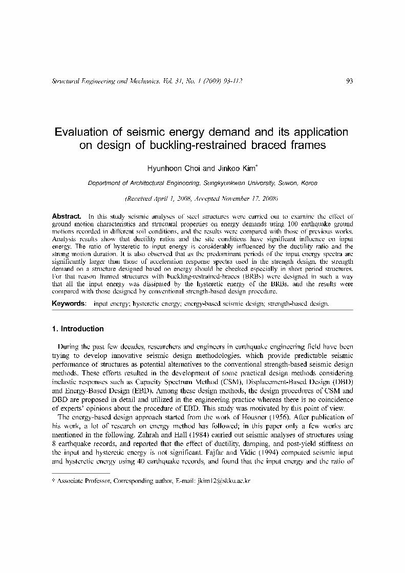
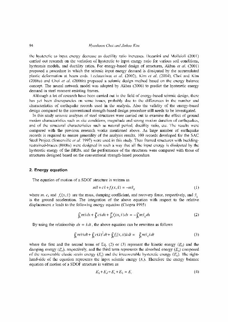
used for the simulation process are described in the SAC Report. Figs. 1 and 2 show the 5%

damped elastic response spectra of the earthquake records utilized.

In the evaluation of the damage accumulated in a structure as a result of an earthquake, the


magnitude of strong motion duration (tsd) of the earthquake is an important factor, which is obtained

as follows (Trifunac and Brady 1975)

(5)

where t0.05 and t0.95 denote the time that the Arias intensity (IA), obtained as follows (Arias 1970),

reaches 5% and 95%, respectively

(6)

where ttd is the total duration of earthquake, g and are the gravity acceleration and the ground

acceleration, respectively. The total and the strong motion durations of the earthquake records used

in the analysis are presented in Table 1 and 2, respectively. The earthquake records with long and

short strong motion duration were identified; for example, in the earthquakes recorded in stiff soil in

Los Angeles; earthquakes with long strong motion duration : LA01, LA02, LA07, LA08, LA09,

tsd t0.95 t0.05–=

IAπ

2g------ x··g

2t( ) td

0

ttd

∫=

x··g

Fig. 1 Response spectra of ground motions developed in SAC Project for LA area

Fig. 2 Response spectra of ground motions developed in SAC Project for Boston area


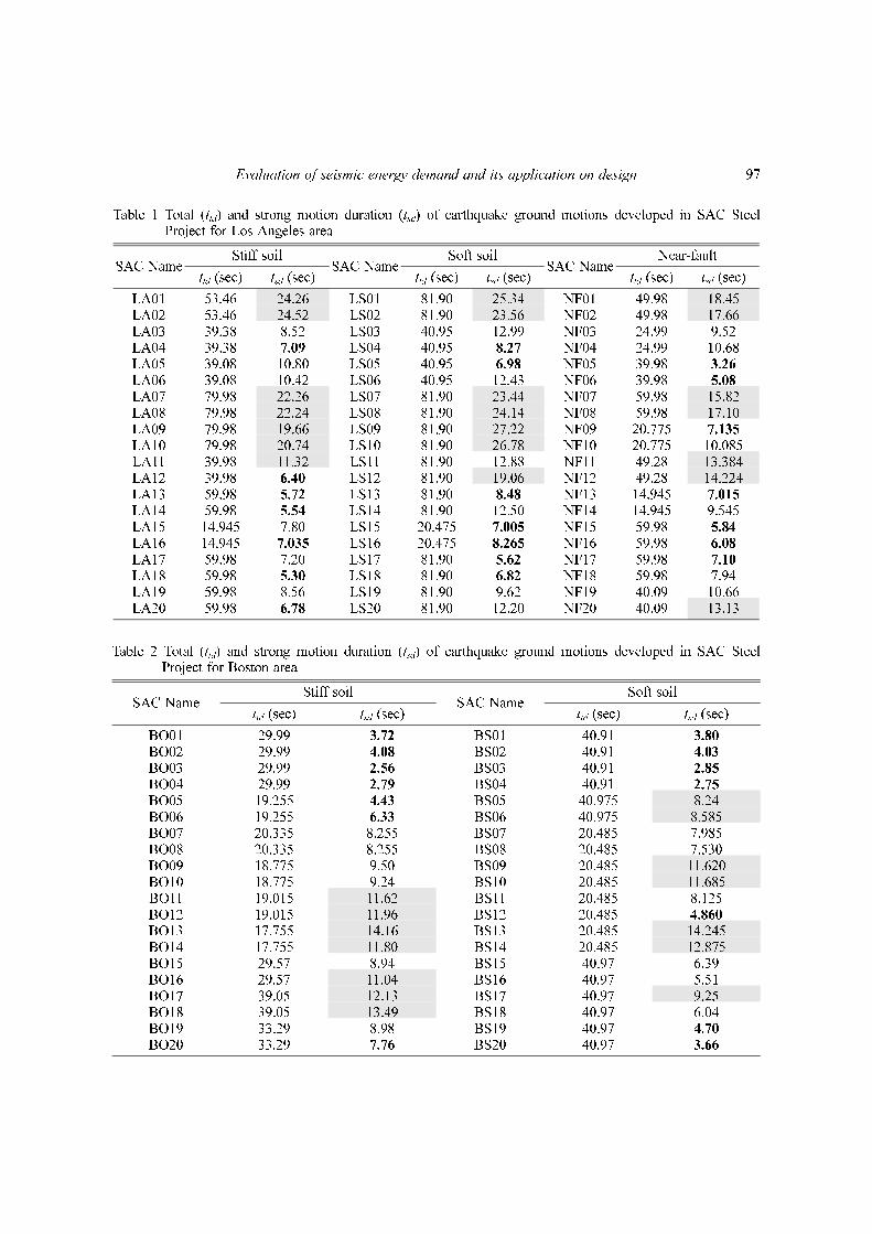
Table 1 Total (ttd) and strong motion duration (tsd) of earthquake ground motions developed in SAC SteelProject for Los Angeles area

SAC NameStiff soil

SAC NameSoft soil

SAC NameNear-fault

ttd (sec) tsd (sec) ttd (sec) tsd (sec) ttd (sec) tsd (sec)

LA01 53.46 24.26 LS01 81.90 25.34 NF01 49.98 18.45LA02 53.46 24.52 LS02 81.90 23.56 NF02 49.98 17.66LA03 39.38 8.52 LS03 40.95 12.99 NF03 24.99 9.52LA04 39.38 7.09 LS04 40.95 8.27 NF04 24.99 10.68LA05 39.08 10.80 LS05 40.95 6.98 NF05 39.98 3.26

LA06 39.08 10.42 LS06 40.95 12.43 NF06 39.98 5.08

LA07 79.98 22.26 LS07 81.90 23.44 NF07 59.98 15.82LA08 79.98 22.24 LS08 81.90 24.14 NF08 59.98 17.10LA09 79.98 19.66 LS09 81.90 27.22 NF09 20.775 7.135

LA10 79.98 20.74 LS10 81.90 26.78 NF10 20.775 10.085LA11 39.98 11.32 LS11 81.90 12.88 NF11 49.28 13.384LA12 39.98 6.40 LS12 81.90 19.06 NF12 49.28 14.224LA13 59.98 5.72 LS13 81.90 8.48 NF13 14.945 7.015

LA14 59.98 5.54 LS14 81.90 12.50 NF14 14.945 9.545LA15 14.945 7.80 LS15 20.475 7.005 NF15 59.98 5.84

LA16 14.945 7.035 LS16 20.475 8.265 NF16 59.98 6.08

LA17 59.98 7.20 LS17 81.90 5.62 NF17 59.98 7.10

LA18 59.98 5.30 LS18 81.90 6.82 NF18 59.98 7.94LA19 59.98 8.56 LS19 81.90 9.62 NF19 40.09 10.66LA20 59.98 6.78 LS20 81.90 12.20 NF20 40.09 13.13

Table 2 Total (ttd) and strong motion duration (tsd) of earthquake ground motions developed in SAC SteelProject for Boston area

SAC NameStiff soil

SAC NameSoft soil

ttd (sec) tsd (sec) ttd (sec) tsd (sec)

BO01 29.99 3.72 BS01 40.91 3.80

BO02 29.99 4.08 BS02 40.91 4.03

BO03 29.99 2.56 BS03 40.91 2.85

BO04 29.99 2.79 BS04 40.91 2.75

BO05 19.255 4.43 BS05 40.975 8.24BO06 19.255 6.33 BS06 40.975 8.585BO07 20.335 8.255 BS07 20.485 7.985BO08 20.335 8.255 BS08 20.485 7.530BO09 18.775 9.50 BS09 20.485 11.620BO10 18.775 9.24 BS10 20.485 11.685BO11 19.015 11.62 BS11 20.485 8.125BO12 19.015 11.96 BS12 20.485 4.860

BO13 17.755 14.16 BS13 20.485 14.245BO14 17.755 11.80 BS14 20.485 12.875BO15 29.57 8.94 BS15 40.97 6.39BO16 29.57 11.04 BS16 40.97 5.51BO17 39.05 12.13 BS17 40.97 9.25BO18 39.05 13.49 BS18 40.97 6.04BO19 33.29 8.98 BS19 40.97 4.70

BO20 33.29 7.76 BS20 40.97 3.66


LA10, and LA11; earthquakes with short strong motion duration : LA04, LA12, LA13, LA14,

LA16, LA18, and LA20. Table 3 presents the average strong motion duration of each set of ground

motions for five different soil conditions.

When sufficient records were not available in the SAC time histories for each soil condition,

broadband strong motions were simulated. According to the research by Teran-Gilmore and Jirsa

(2004) using long duration narrow-banded ground motions recorded in the lake zone of Mexico

City, which have predominant period around 2.0 sec, the maximum plastic energy demands for

Mexico soft soil are about two to three times larger than those for the SAC ground motions for LA

area. Bojórquez and Ruiz (2004) also utilized the narrow-band motions recorded in the Valley of

Mexico to investigate the effect of low-cycle fatigue on the ductility capacity. These results obtained

from narrow-band motions recorded in very soft soil were compared with those obtained from SAC

records.

3.2 Input energy and hysteretic energy

From analyses using 8 earthquake records, Zahrah and Hall (1984) concluded that ductility

demand (μ) does not have a significant influence on the earthquake input energy (Ei). Uang and

Bertero (1988) also showed that the input energy spectra are generally insensitive to the level of

ductility ratio for El Centro record (1940, N00E) and San Salvador record (1986, N90E). More

researchers (Akiyama 1985, Nakashima et al. 1996) reported similar observations. Based on the

assumption that input energy is independent of system parameters such as viscous damping,

ductility and strength level, Cruz and López (2000) suggested simple expressions of the plastic

energy, expressed as a fraction of the input energy, calculated in terms of normalized input power,

which incorporates five single-degree-of-freedom (SDOF) and two multi-degree-of-freedom

(MDOF) structures. However, according to the analysis results using mean response of 40

earthquake records by Fajfar and Vidic (1994), the input energy decreases as ductility increases for

period range larger than about 0.4 second. On the other hand, though the input energy was not

much affected by the change of ductility for short periods less than 0.4 second, it was observed that

the input energy increases as ductility increases. Also Decanini and Mollaioli (2001) showed that

ductility has a significant influence on input energy. Using 10 earthquake records each with short

and long duration of strong motion, Khashaee et al. (2003) concluded that as the ductility increases,

the influence of the duration of strong motion on the input energy spectra becomes more significant,

particularly in the vicinity of the predominant period.

It can be observed in the review of the previous research that there is inconsistency whether

ductility has a negligible effect on input energy or not. Much part of the discrepancy is originated

from how the results were obtained; e.g. results from individual record or from averaging many

results obtained from individual records. Considering the non-stationary nature of earthquakes, it

Table 3 Average strong motion duration of each set of ground motions

Area LA Boston

Soil type Stiff soil Soft soil Near-fault Stiff soil Soft soil

Set of 20 earthquake records (sec) 12.11 14.68 10.49 8.56 7.24

Long strong motion duration (sec) 20.71 24.22 15.68 12.31 10.93

Short strong motion duration (sec) 6.27 7.35 5.93 4.52 3.81


seems to be more reasonable to use mean values using ensemble of earthquake records in the

investigation of the effect of various parameters on the seismic input and hysteretic energy. In this

study the input and hysteretic energy were computed for 100 SDOF systems using the nonlinear

analysis program code NONSPEC (Mahin and Lin 1983). The analysis model structures, the natural

period of which ranges from 0.05 second to 5.0 second, have bi-linear force-displacement

relationship with zero post-yield stiffness. Damping ratio was assumed to be 5% of the critical

damping. Time-history analyses were carried out and the energy responses for the 20 earthquakes in

each site condition were averaged. For SDOF structures with various natural periods and target

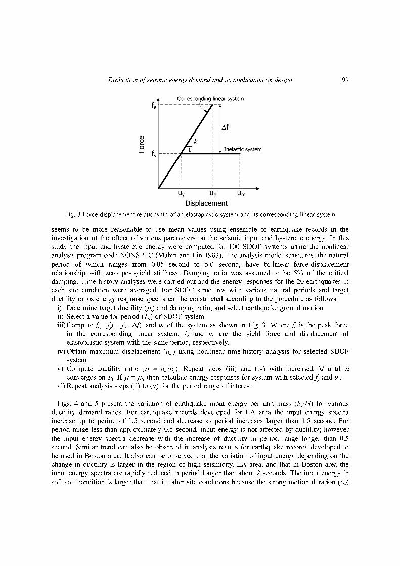
ductility ratios energy response spectra can be constructed according to the procedure as follows:

i) Determine target ductility (μt) and damping ratio, and select earthquake ground motion

ii) Select a value for period (Tn) of SDOF system

iii) Compute fe, and uy of the system as shown in Fig. 3. Where fe is the peak force

in the corresponding linear system, fy and uy are the yield force and displacement of

elastoplastic system with the same period, respectively.

iv) Obtain maximum displacement (um) using nonlinear time-history analysis for selected SDOF

system.

v) Compute ductility ratio (μ = um/uy). Repeat steps (iii) and (iv) with increased Δf until μ

converges on μt. If μ = μt, then calculate energy responses for system with selected fy and uy.

vi) Repeat analysis steps (ii) to (v) for the period range of interest.

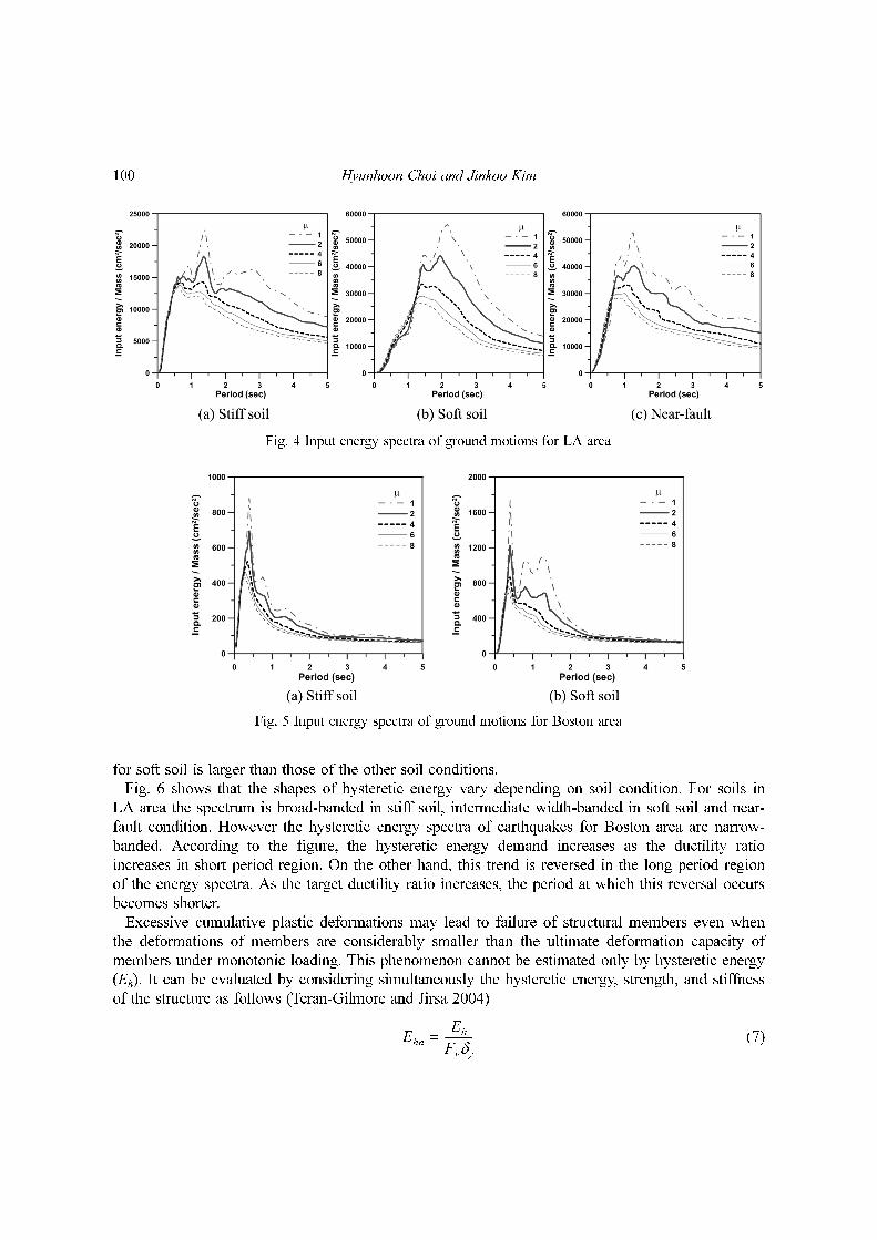
Figs. 4 and 5 present the variation of earthquake input energy per unit mass (Ei/M) for various

ductility demand ratios. For earthquake records developed for LA area the input energy spectra

increase up to period of 1.5 second and decrease as period increases larger than 1.5 second. For

period range less than approximately 0.5 second, input energy is not affected by ductility; however

the input energy spectra decrease with the increase of ductility in period range longer than 0.5

second. Similar trend can also be observed in analysis results for earthquake records developed to

be used in Boston area. It also can be observed that the variation of input energy depending on the

change in ductility is larger in the region of high seismicity, LA area, and that in Boston area the

input energy spectra are rapidly reduced in period longer than about 2 seconds. The input energy in

soft soil condition is larger than that in other site conditions because the strong motion duration (tsd)

fy fe fΔ–=( )

Fig. 3 Force-displacement relationship of an elastoplastic system and its corresponding linear system


for soft soil is larger than those of the other soil conditions.

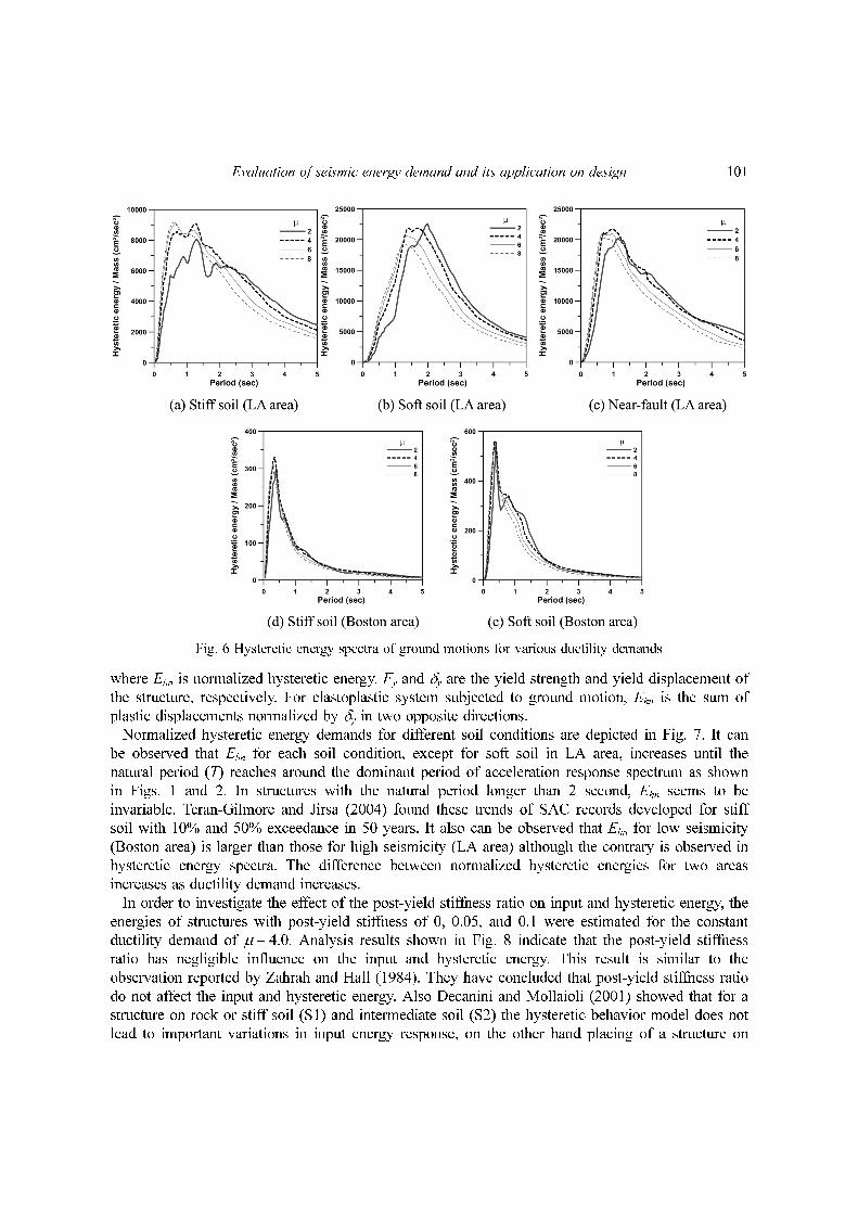
Fig. 6 shows that the shapes of hysteretic energy vary depending on soil condition. For soils in

LA area the spectrum is broad-banded in stiff soil, intermediate width-banded in soft soil and near-

fault condition. However the hysteretic energy spectra of earthquakes for Boston area are narrow-

banded. According to the figure, the hysteretic energy demand increases as the ductility ratio

increases in short period region. On the other hand, this trend is reversed in the long period region

of the energy spectra. As the target ductility ratio increases, the period at which this reversal occurs

becomes shorter.

Excessive cumulative plastic deformations may lead to failure of structural members even when

the deformations of members are considerably smaller than the ultimate deformation capacity of

members under monotonic loading. This phenomenon cannot be estimated only by hysteretic energy

(Eh). It can be evaluated by considering simultaneously the hysteretic energy, strength, and stiffness

of the structure as follows (Teran-Gilmore and Jirsa 2004)

(7)Ehn

Eh

Fyδy

----------=

Fig. 4 Input energy spectra of ground motions for LA area

Fig. 5 Input energy spectra of ground motions for Boston area


where Ehn is normalized hysteretic energy. Fy and δy are the yield strength and yield displacement of

the structure, respectively. For elastoplastic system subjected to ground motion, Ehn is the sum of

plastic displacements normalized by δy in two opposite directions.

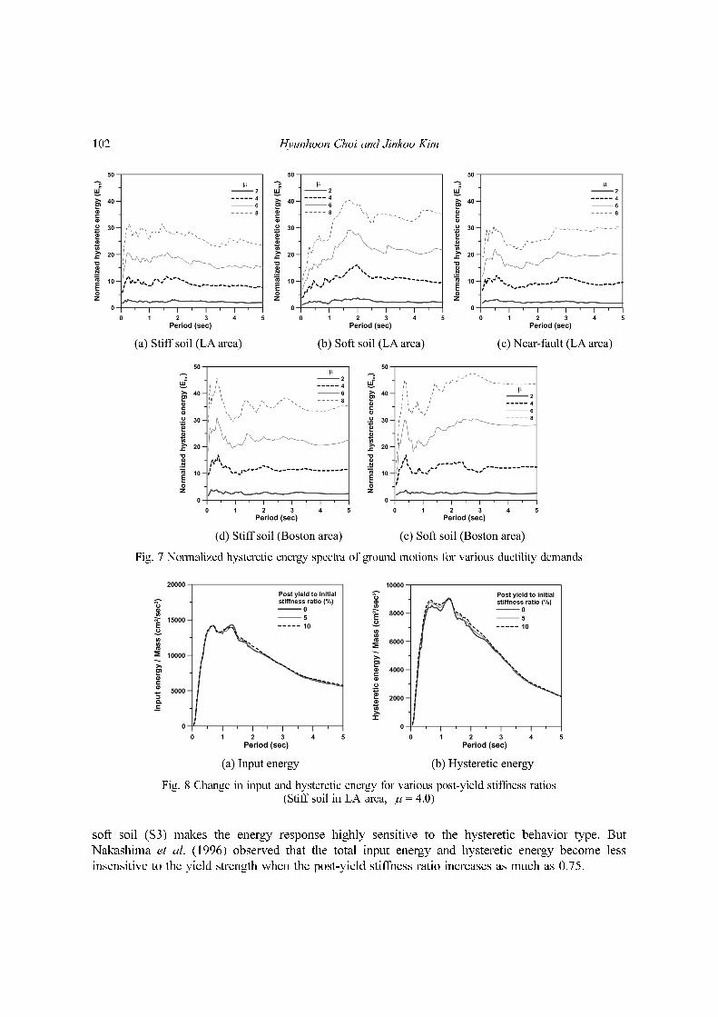
Normalized hysteretic energy demands for different soil conditions are depicted in Fig. 7. It can

be observed that Ehn for each soil condition, except for soft soil in LA area, increases until the

natural period (T) reaches around the dominant period of acceleration response spectrum as shown

in Figs. 1 and 2. In structures with the natural period longer than 2 second, Ehn seems to be

invariable. Teran-Gilmore and Jirsa (2004) found these trends of SAC records developed for stiff

soil with 10% and 50% exceedance in 50 years. It also can be observed that Ehn for low seismicity

(Boston area) is larger than those for high seismicity (LA area) although the contrary is observed in

hysteretic energy spectra. The difference between normalized hysteretic energies for two areas

increases as ductility demand increases.

In order to investigate the effect of the post-yield stiffness ratio on input and hysteretic energy, the

energies of structures with post-yield stiffness of 0, 0.05, and 0.1 were estimated for the constant

ductility demand of μ = 4.0. Analysis results shown in Fig. 8 indicate that the post-yield stiffness

ratio has negligible influence on the input and hysteretic energy. This result is similar to the

observation reported by Zahrah and Hall (1984). They have concluded that post-yield stiffness ratio

do not affect the input and hysteretic energy. Also Decanini and Mollaioli (2001) showed that for a

structure on rock or stiff soil (S1) and intermediate soil (S2) the hysteretic behavior model does not

lead to important variations in input energy response, on the other hand placing of a structure on

Fig. 6 Hysteretic energy spectra of ground motions for various ductility demands


soft soil (S3) makes the energy response highly sensitive to the hysteretic behavior type. But

Nakashima et al. (1996) observed that the total input energy and hysteretic energy become less

insensitive to the yield strength when the post-yield stiffness ratio increases as much as 0.75.

Fig. 7 Normalized hysteretic energy spectra of ground motions for various ductility demands

Fig. 8 Change in input and hysteretic energy for various post-yield stiffness ratios (Stiff soil in LA area, μ = 4.0)


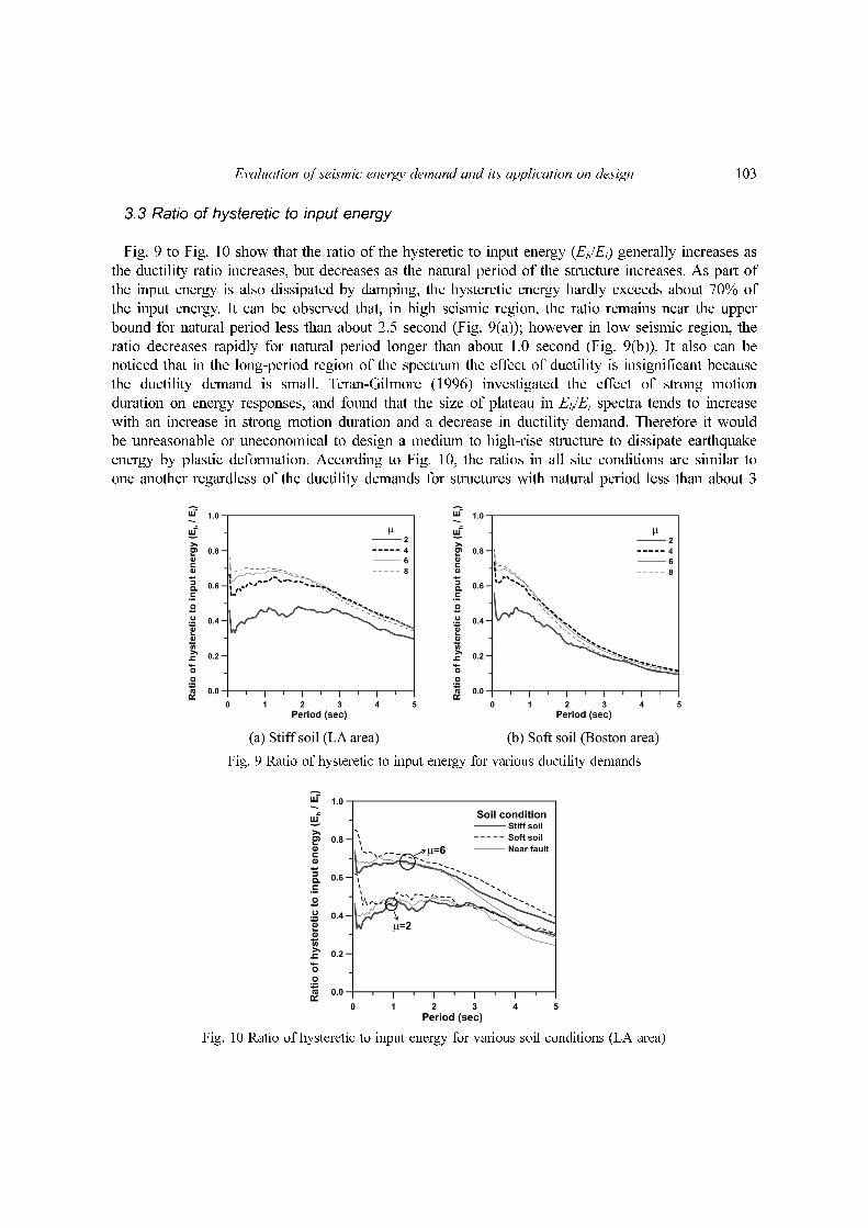
3.3 Ratio of hysteretic to input energy

Fig. 9 to Fig. 10 show that the ratio of the hysteretic to input energy (Eh/Ei) generally increases as

the ductility ratio increases, but decreases as the natural period of the structure increases. As part of

the input energy is also dissipated by damping, the hysteretic energy hardly exceeds about 70% of

the input energy. It can be observed that, in high seismic region, the ratio remains near the upper

bound for natural period less than about 2.5 second (Fig. 9(a)); however in low seismic region, the

ratio decreases rapidly for natural period longer than about 1.0 second (Fig. 9(b)). It also can be

noticed that in the long-period region of the spectrum the effect of ductility is insignificant because

the ductility demand is small. Teran-Gilmore (1996) investigated the effect of strong motion

duration on energy responses, and found that the size of plateau in Eh/Ei spectra tends to increase

with an increase in strong motion duration and a decrease in ductility demand. Therefore it would

be unreasonable or uneconomical to design a medium to high-rise structure to dissipate earthquake

energy by plastic deformation. According to Fig. 10, the ratios in all site conditions are similar to

one another regardless of the ductility demands for structures with natural period less than about 3

Fig. 9 Ratio of hysteretic to input energy for various ductility demands

Fig. 10 Ratio of hysteretic to input energy for various soil conditions (LA area)


seconds, whereas the ratios of the records developed for near-fault condition become smaller than

those of the records corresponding to the other site conditions when the natural periods are larger

than 3 seconds. This result, however, does not correspond with the results of Khashaee et al. (2003)

obtained using 20 records, which show that the ratios remain nearly constant when the ductility

demand varies from 2 to 5. The discrepancy seems to be resulted from the fact that the energy

ratios presented in their study were average values of the results computed using earthquakes with

various soil conditions. Decanini and Mollaioli (2001) also found that the ductility ratio and the soil

condition affect the ratio significantly.

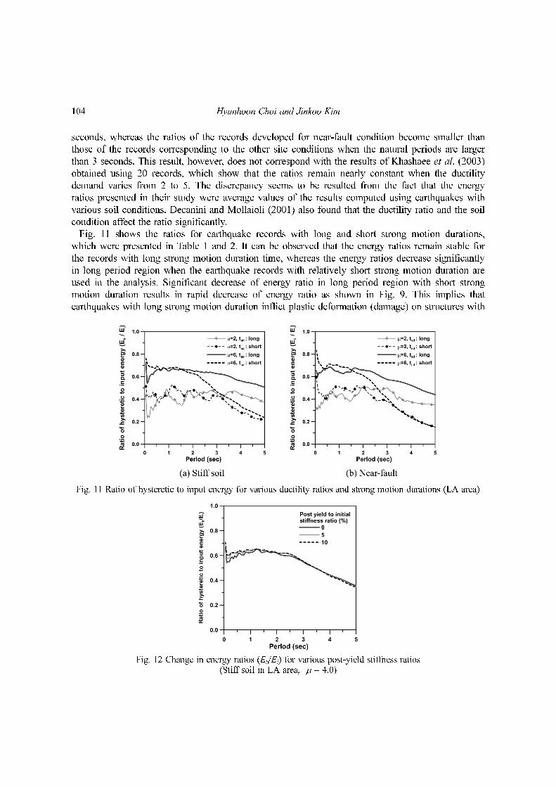
Fig. 11 shows the ratios for earthquake records with long and short strong motion durations,

which were presented in Table 1 and 2. It can be observed that the energy ratios remain stable for

the records with long strong motion duration time, whereas the energy ratios decrease significantly

in long period region when the earthquake records with relatively short strong motion duration are

used in the analysis. Significant decrease of energy ratio in long period region with short strong

motion duration results in rapid decrease of energy ratio as shown in Fig. 9. This implies that

earthquakes with long strong motion duration inflict plastic deformation (damage) on structures with

Fig. 11 Ratio of hysteretic to input energy for various ductility ratios and strong motion durations (LA area)

Fig. 12 Change in energy ratios (Eh/Ei) for various post-yield stiffness ratios (Stiff soil in LA area, μ = 4.0)


wide spectrum of natural periods, whereas those with short strong motion duration damage

structures with only short natural periods. Fig. 12 shows the effect of post-yield stiffness on the

ratio, where it can be noticed that the ratio is not affected by the post-yield stiffness. Therefore it

can be concluded that as the ratio remains stable regardless of the site conditions in structures with

up to medium natural periods, the quantity can be used as a reliable design parameter in energy-

based seismic design.

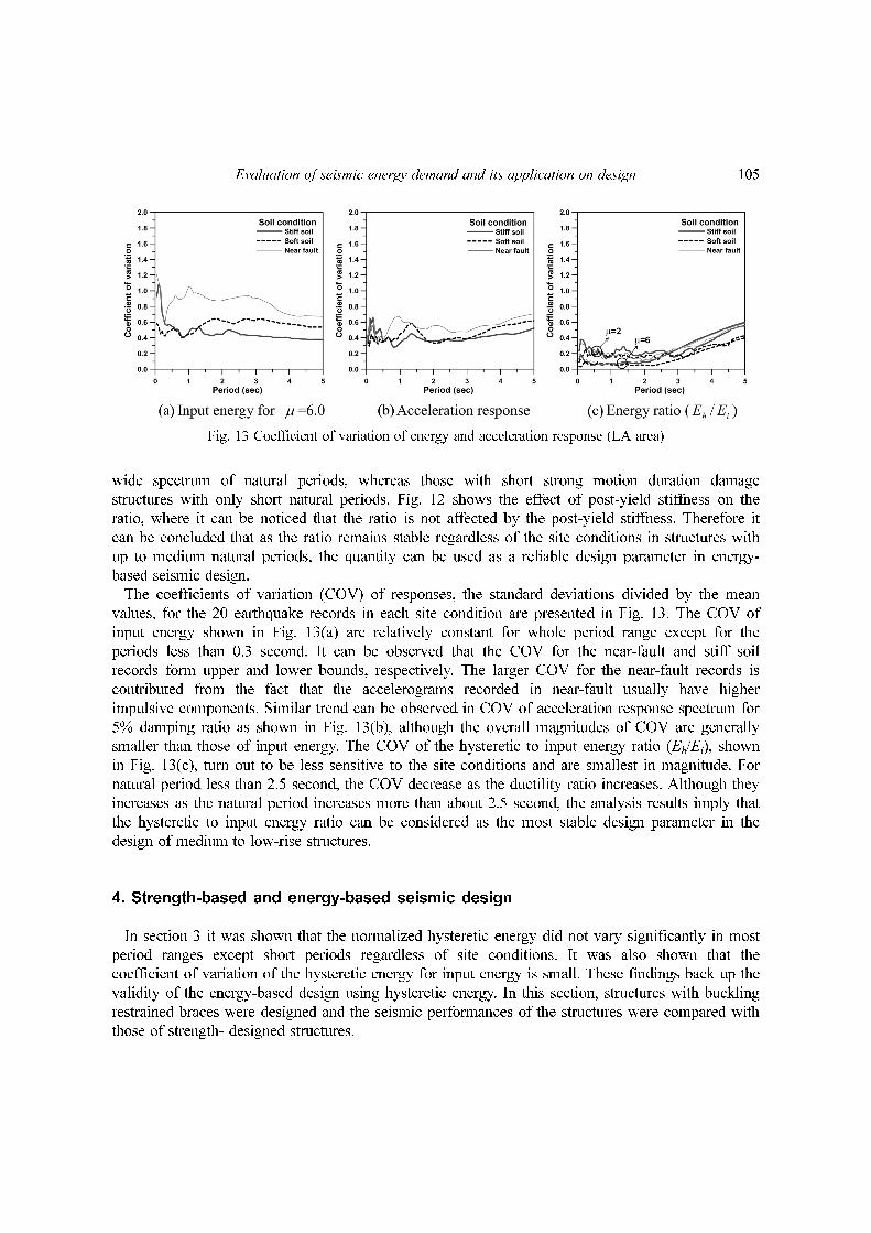
The coefficients of variation (COV) of responses, the standard deviations divided by the mean

values, for the 20 earthquake records in each site condition are presented in Fig. 13. The COV of

input energy shown in Fig. 13(a) are relatively constant for whole period range except for the

periods less than 0.3 second. It can be observed that the COV for the near-fault and stiff soil

records form upper and lower bounds, respectively. The larger COV for the near-fault records is

contributed from the fact that the accelerograms recorded in near-fault usually have higher

impulsive components. Similar trend can be observed in COV of acceleration response spectrum for

5% damping ratio as shown in Fig. 13(b), although the overall magnitudes of COV are generally

smaller than those of input energy. The COV of the hysteretic to input energy ratio (Eh/Ei), shown

in Fig. 13(c), turn out to be less sensitive to the site conditions and are smallest in magnitude. For

natural period less than 2.5 second, the COV decrease as the ductility ratio increases. Although they

increases as the natural period increases more than about 2.5 second, the analysis results imply that

the hysteretic to input energy ratio can be considered as the most stable design parameter in the

design of medium to low-rise structures.

4. Strength-based and energy-based seismic design

In section 3 it was shown that the normalized hysteretic energy did not vary significantly in most

period ranges except short periods regardless of site conditions. It was also shown that the

coefficient of variation of the hysteretic energy for input energy is small. These findings back up the

validity of the energy-based design using hysteretic energy. In this section, structures with buckling

restrained braces were designed and the seismic performances of the structures were compared with

those of strength- designed structures.

Fig. 13 Coefficient of variation of energy and acceleration response (LA area)


4.1 Pseudo-acceleration and energy spectra

According to the pseudo-acceleration spectra of the ground motions used in the analyses (Fig. 1

and Fig. 2), the maximum values generally occur at the short-period region, except for a few

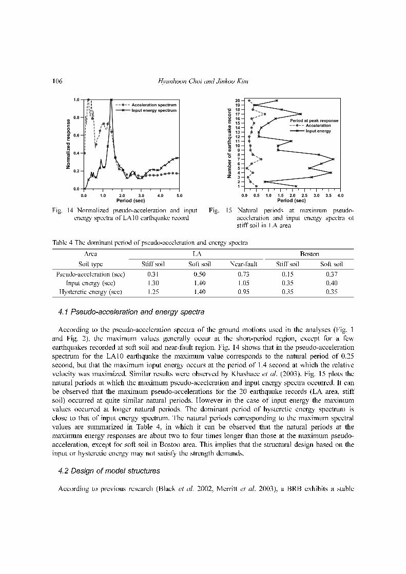
earthquakes recorded at soft soil and near-fault region. Fig. 14 shows that in the pseudo-acceleration

spectrum for the LA10 earthquake the maximum value corresponds to the natural period of 0.25

second, but that the maximum input energy occurs at the period of 1.4 second at which the relative

velocity was maximized. Similar results were observed by Khashaee et al. (2003). Fig. 15 plots the

natural periods at which the maximum pseudo-acceleration and input energy spectra occurred. It can

be observed that the maximum pseudo-accelerations for the 20 earthquake records (LA area, stiff

soil) occurred at quite similar natural periods. However in the case of input energy the maximum

values occurred at longer natural periods. The dominant period of hysteretic energy spectrum is

close to that of input energy spectrum. The natural periods corresponding to the maximum spectral

values are summarized in Table 4, in which it can be observed that the natural periods at the

maximum energy responses are about two to four times longer than those at the maximum pseudo-

acceleration, except for soft soil in Boston area. This implies that the structural design based on the

input or hysteretic energy may not satisfy the strength demands.

4.2 Design of model structures

According to previous research (Black et al. 2002, Merritt et al. 2003), a BRB exhibits a stable

Fig. 14 Normalized pseudo-acceleration and inputenergy spectra of LA10 earthquake record

Fig. 15 Natural periods at maximum pseudo-acceleration and input energy spectra ofstiff soil in LA area

Table 4 The dominant period of pseudo-acceleration and energy spectra

Area LA Boston

Soil type Stiff soil Soft soil Near-fault Stiff soil Soft soil

Pseudo-acceleration (sec) 0.31 0.50 0.73 0.15 0.37

Input energy (sec) 1.30 1.40 1.05 0.35 0.40

Hysteretic energy (sec) 1.25 1.40 0.95 0.35 0.35


hysteretic behavior with excellent energy dissipation capacity both in tension and compression. A

steel casing and mortar filler are used to provide lateral support to the core element and to prevent

global and local buckling of the steel core when compressive force is applied. Consequently the

hysteretic behavior of BRB can easily be modeled and the amount of dissipated energy can be

computed using simple equations (Choi et al. 2006b). To compare the seismic performance of

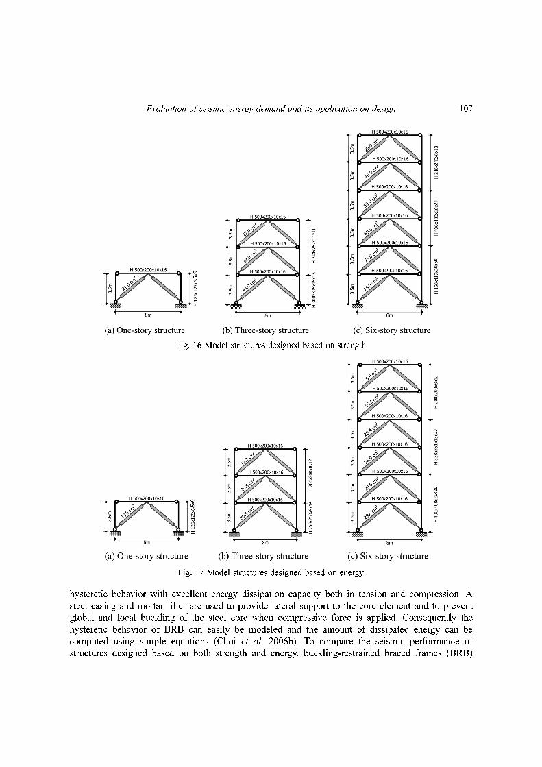
structures designed based on both strength and energy, buckling-restrained braced frames (BRB)

Fig. 16 Model structures designed based on strength

Fig. 17 Model structures designed based on energy


were prepared. The 1, 3, and 6 story-structures have 3.5m story height and 8m bay length. As

shown in Figs. 16 and 17 the girders are pin-connected to columns, and only the BRBs dissipate

seismic energy through plastic deformation. The design dead and live loads of 4.9kN/m2 and

2.45kN/m2, respectively, were used for design. The inherent modal damping ratios for dynamic

analysis were assumed to be 5% of the critical damping in the first and the second modes.

For strength based design of BRB frames, the seismic load was computed using the mean

response spectrum presented in Fig. 1(a), in which the seismic coefficients SDS and SD1 in the IBC

2006 format are estimated to be 1.375 and 0.77, respectively. The importance factor of 1.25 was

used to obtain design base shear. Beams and columns were designed per the AISC Load and

Resistance Factor Design (1999) and the Seismic Provisions for Structural Steel Buildings (2002).

The BRBs were designed per Chapter 8 of the FEMA-450 (BSSC 2004), in which the response

modification factor of buckling-restrained braced frames is specified as 7. The yield stress of the

structural steel is 240 MPa. In the strength-based design the ratio of stress demand to capacity is

kept above 0.9 for beams and columns and especially above 0.95 for BRBs. The steel core areas of

BRBs were calculated using the following relation suggested in the FEMA-450

(8)

where Pu is the required axial strength and φ is the strength reduction factor, which is 0.9.

is the design strength, where Fy and Asc are the specified minimum yield strength and

net area of steel core, respectively.

For energy based design of BRB frame, the procedure proposed previously by the authors (2006a)

was followed: The target displacement (1.5% of story height) and the ductility ratio (μt = 6.5 for all

stories) at the target displacement were determined first. Then the hysteretic energy spectrum and

the accumulated ductility spectrum corresponding to the ductility ratio (μt) were constructed, and the

hysteretic energy (Eh) and the accumulated ductility ratio (μa) corresponding to the natural period of

the model structures were obtained. The accumulated ductility ratio μa is the sum of the positive

and negative yield excursions. By assuming that all the seismic input energy is dissipated by BRBs,

the cross-sectional area of BRBs located in the first story can be computed as follows

(9a)

(9b)

where Eh, Fyj, uyj, and μa are the hysteretic energy normalized by mass obtained from the spectrum,

the yield force of the jth story, the yield displacement of the jth story, and the accumulated ductility

ratio, respectively. For model structures the values of μa range approximately from 20 to 23. Also

Abj and Lbj are the cross-sectional area and length of BRB located on the jth story, respectively. σbj

and Eb are yield stress and elastic modulus of BRB, respectively. mi is the mass of the ith story. The

cross-sectional area of BRB located in the jth story, Abj, is denoted as the cross-sectional area of

BRB in the first story, Ab1, multiplied by the story-wise distribution ratio, Dj

(10)

Pu φPysc≤

Pysc FyAsc=

Eh mi

i 1=

N

∑× Fyj

j 1=

N

∑ uyj μa 1–( ) μa 1–( ) Abjσby

Lbjσby

Eb

--------------j 1=

N

∑= =

Ab1

Eh mi

i 1=

N

∑

μa 1–( ) Djσby

Lbjσby

Eb

--------------j 1=

N

∑

------------------------------------------------------=

Abj DjAb1=


In this study it is assumed that the hysteretic energy is distributed in each story proportional to the

story-wise distribution ratio of hysteretic energy obtained from nonlinear dynamic analysis. Figs. 16

and 17 show the size of structural members selected using the code-based and the energy-based

procedures, respectively.

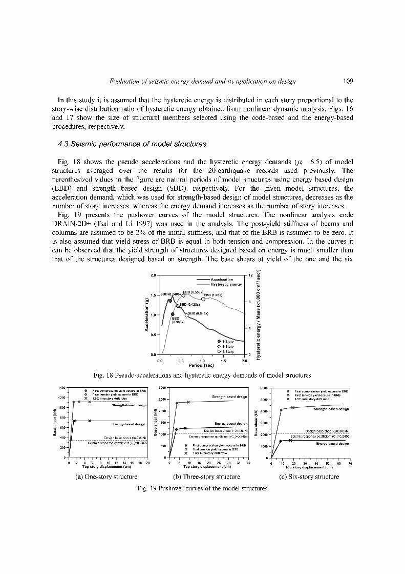
4.3 Seismic performance of model structures

Fig. 18 shows the pseudo accelerations and the hysteretic energy demands (μt = 6.5) of model

structures averaged over the results for the 20-earthquake records used previously. The

parenthesized values in the figure are natural periods of model structures using energy based design

(EBD) and strength based design (SBD), respectively. For the given model structures, the

acceleration demand, which was used for strength-based design of model structures, decreases as the

number of story increases, whereas the energy demand increases as the number of story increases.

Fig. 19 presents the pushover curves of the model structures. The nonlinear analysis code

DRAIN-2D+ (Tsai and Li 1997) was used in the analysis. The post-yield stiffness of beams and

columns are assumed to be 2% of the initial stiffness, and that of the BRB is assumed to be zero. It

is also assumed that yield stress of BRB is equal in both tension and compression. In the curves it

can be observed that the yield strength of structures designed based on energy is much smaller than

that of the structures designed based on strength. The base shears at yield of the one and the six

Fig. 19 Pushover curves of the model structures

Fig. 18 Pseudo-accelerations and hysteretic energy demands of model structures


story energy-designed structures are only 66% and 35%, respectively, of the strength-designed

structures. The over-strength factors, the ratio of the yield to design stress, are 3.20 (1-story), 2.24

(3-story), and 1.97 (6-story) for strength-designed structures, which are larger than or equal to the

over-strength factor of 2.0 specified in the FEMA-450 (BSSC 2004). However the over-strength

factors of the structures designed based on energy are 2.10 (1-story), 1.16 (3-story), and 0.69 (6-

story), which are significantly smaller than those of the strength-designed structures. The smaller

overstrength factors of the structures designed based on energy are partly contributed from the fact

that the structures are more optimally designed in such a way that structural damages are more

uniformly distributed throughout the stories. Another important factor is that the strength reduction

factors and load factors were not used in the energy-based design, whereas they were applied in the

code-based strength-design.

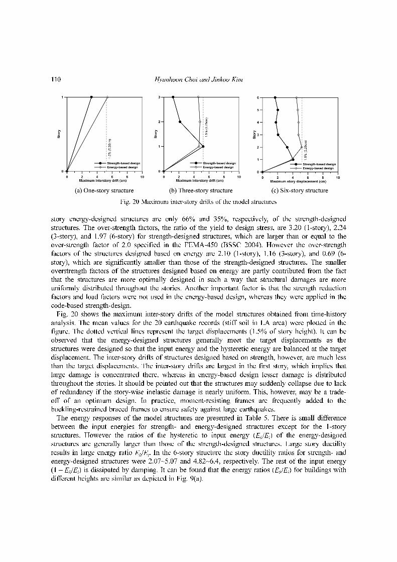
Fig. 20 shows the maximum inter-story drifts of the model structures obtained from time-history

analysis. The mean values for the 20 earthquake records (stiff soil in LA area) were plotted in the

figure. The dotted vertical lines represent the target displacements (1.5% of story height). It can be

observed that the energy-designed structures generally meet the target displacements as the

structures were designed so that the input energy and the hysteretic energy are balanced at the target

displacement. The inter-story drifts of structures designed based on strength, however, are much less

than the target displacements. The inter-story drifts are largest in the first story, which implies that

large damage is concentrated there, whereas in energy-based design lesser damage is distributed

throughout the stories. It should be pointed out that the structures may suddenly collapse due to lack

of redundancy if the story-wise inelastic damage is nearly uniform. This, however, may be a trade-

off of an optimum design. In practice, moment-resisting frames are frequently added to the

buckling-restrained braced frames to ensure safety against large earthquakes.

The energy responses of the model structures are presented in Table 5. There is small difference

between the input energies for strength- and energy-designed structures except for the 1-story

structures. However the ratios of the hysteretic to input energy (Eh/Ei) of the energy-designed

structures are generally larger than those of the strength-designed structures. Large story ductility

results in large energy ratio Eh/Ei. In the 6-story structure the story ductility ratios for strength- and

energy-designed structures were 2.07~5.07 and 4.82~6.4, respectively. The rest of the input energy

(1 − Eh/Ei) is dissipated by damping. It can be found that the energy ratios (Eh/Ei) for buildings with

different heights are similar as depicted in Fig. 9(a).

Fig. 20 Maximum inter-story drifts of the model structures


5. Conclusions

In this study the influences of ground motion characteristics and structural properties on energy

demands were evaluated using 100 earthquake ground motions recorded in different soil conditions,

and the results were compared with those of previous works. Then framed structures with buckling-

restrained-braces (BRBs) were designed in such a way that all the input energy is dissipated by the

hysteretic energy of the BRBs, and the results were compared with those designed by conventional

strength-based design procedure.

The analytical results showed that ductility ratios and the site conditions had significant influence

on the input energy. The ratio of hysteretic to input energy was considerably affected by the

ductility ratio and the strong motion duration. The evaluation of normalized hysteretic energy

demands (Ehn) for different soil conditions showed that Ehn for low seismicity (Boston area) was

larger than those for high seismicity (LA area) although the opposite was observed in hysteretic

energy spectra. Therefore hysteretic energy in itself may not provide enough information about the

damage caused by accumulated yield excursions. In the comparison of pseudo-acceleration and

energy spectra, it was found that the natural periods corresponding to the maximum energy response

were about two to four times longer than those at the maximum pseudo-acceleration. This implies

that the structural design based on the energy demand may not satisfy the strength demand. The

static and dynamic nonlinear analyses of both strength-designed and energy-designed structures

showed that the energy-based design, which is basically performance-based, resulted in smaller

member size, smaller strength, and more damage compared to structures designed based on strength.

Therefore if a structure, designed based on energy, is to meet both strength and displacement

criteria, it is necessary to check strength after it is designed based on energy, as the strength-based

design requires displacement check afterwards.

References

AISC (1999), Load and Resistance Factor Design Specification for Structural Steel Buildings, American Instituteof Steel Construction, Chicago, IL.

AISC (2002), Seismic Provisions for Structural Steel Buildings, American Institute of Steel Construction,Chicago, IL.

Akbas, B. (2006), “A neural network model to assess the hysteretic energy demand in steel moment resistingframes”, Struct. Eng. Mech., 23(2), 177-193.

Akbas, B., Shen, J. and Hao, H. (2001), “Energy approach in performance-based seismic design of steel momentresisting frames for basic safety objective”, Struct. Des. Tall Build., 10(3), 193-217.

Akiyama, H. (1985), Earthquake-resistant Limit-state Design for Buildings, University of Tokyo Press, Japan.Arias, A. (1970), “A measure of earthquake intensity”, in Seismic Design for Nuclear Power Plants, ed. R.J.

Table 5 Energy responses of model structures

Story

Strength based design Energy based design

Input energy/mass(cm2/sec2)

Eh /Ei

Input energy/mass(cm2/sec2)

Eh /Ei

1 Story 7024 0.446 9251 0.596

3 Story 10615 0.504 11345 0.647

6 Story 12099 0.460 11624 0.654


Hansen, Massachusetts Institute of Technology Press, 438-469.Black, C., Makris, N. and Aiken, I. (2002), “Component testing, stability analysis and characterization of

buckling restrained braces”, PEER Report 2002/08, Pacific Earthquake Engineering Research Center,University of California, Berkeley.

Bojórquez, E. and Ruiz, S.E. (2004), “Strength reduction factors for the Valley of Mexico, considering low-cyclefatigue effects”, 13th World Conference on Earthquake Engineering, Vancouver, Canada, Paper No. 516.

Bruneau, M. and Wang, N. (1996), “Some aspects of energy methods for the inelastic seismic response of ductileSDOF structures”, Eng. Struct., 18(1), 1-12.

Building Seismic Safety Council (2004), “NEHRP Recommended provisions for seismic regulations for newbuildings and other structures, 2003 Edition, Part 1: Provisions”, Report No. FEMA-450, Federal EmergencyManagement Agency, Washington, D.C.

Choi, H. and Kim, J. (2006a), “Energy-based seismic design of buckling-restrained braced frames usinghysteretic energy spectrum”, Eng. Struct., 28(2), 304-311.

Choi, H., Kim, J. and Chung, L. (2006b), “Seismic design of buckling-restrained braced frames based on amodified energy-balance concept”, Can. J. Civil Eng., 33(10), 1251-1260.

Chopra, A.K. (1995), Dynamics of Structures: Theory and Applications to Earthquake Engineering, Prentice HallInc., New Jersey.

Cruz, M.F. and López, O.A. (2000), “Plastic energy dissipated during an earthquake as a function of structuralproperties and ground motion characteristics”, Eng. Struct., 22(7), 784-792.

Decanini, L.D. and Mollaioli, F. (2001), “An energy-based methodology for the assessment of seismic demand”,Soil Dyn. Earthq. Eng., 21(2), 113-137.

Fajfar, P. and Vidic, T. (1994), “Consistent inelastic design spectra: Hysteretic and input energy”, Earthq. Eng.Struct. Dyn., 23(5), 523-537.

Housner, G.W. (1956), “Limit design of structures to resist earthquakes”, Proceedings of the First WorldConference on Earthquake Engineering, Berkeley, California.

ICC (2006), 2006 International Building Code, International Code Council Inc., Country Club Hills, IL.Khashaee, P., Mohraz, B., Sadek, F., Lew, H.S. and Gross, J.L. (2003), “Distribution of earthquake input energy

in structures”, Report No. NISTIR 6903, National Institute of Standards and Technology, Washington.Kim, J., Choi, H. and Chung, L. (2004), “Energy-based seismic design of structures with buckling-restrained

braces”, Steel Compos. Struct., 4(6), 437-452.Leelataviwat, S., Goel, S.C. and Stojadinovi, B. (2002), “Energy-based seismic design of structures using yield

mechanism and target drift”, J. Struct. Eng., 128(8), 1046-1054.Mahin, S.A. and Lin, J. (1983), “Inelastic response spectra for single degree of freedom systems”, Department of

Civil Engineering, University of California, Berkeley.Merritt, S., Uang, C.M. and Benzoni, G. (2003), “Subassemblage testing of corebrace buckling-restrained

braces”, Report No. TR-2003/01, University of California, San Diego.Nakashima, M., Saburi, K. and Tsuji, B. (1996), “Energy input and dissipation behaviour of structures with

hysteretic dampers”, Earthq. Eng. Struct. Dyn., 25(5), 483-496.Somerville, P., Smith, H., Puriyamurthala, S. and Sun, J. (1997), “Development of Ground Motion Time

Histories for Phase 2 of the FEMA/SAC Steel Project”, SAC Joint Venture, SAC/BD 97/04.Teran-Gilmore, A. (1996), “Performance-based earthquake-resistant design of framed buildings using energy

concept”, Ph. D. Thesis, University of California at Berkeley.Teran-Gilmore, A. and Jirsa, J.O. (2004), “The use of cumulative ductility strength spectra for seismic design against

low cycle fatigue”, 13th World Conference on Earthquake Engineering, Vancouver, Canada, Paper No. 889.Trifunac, M.D. and Brady, A.G. (1975), “A study on the duration of strong earthquake ground motion,” B.

Seismol. Soc. Am., 65(3), 581-626.Tsai, K.C. and Li, J.W. (1997), “DRAIN2D+, A general purpose computer program for static and dynamic

analyses of inelastic 2D structures supplemented with a graphic processor”, Report No. CEER/R86-07,National Taiwan University, Taipei, Taiwan.

Uang, C.M. and Bertero, V.V. (1988), “Use of energy as a design criterion in earthquake-resistant design”,Report No. UCB/EERC-88/18, Earthquake Engineering Research Center, University of California at Berkeley.

Zahrah, T. and Hall, J. (1984), “Earthquake energy absorption in SDOF structures”, J. Struct. Eng., 110(8), 1757-1772.

Documents

Evaluation of seismic energy demand and its application … of seismic energy demand and its application on design 95 The energy in the above equation is the relative energy based