EVALUATION OF STEWART'S MODEL FOR ACID-BASE BALANCED PATIENTS

WITH DIABETIC KETOACIDOSIS

Janice Errela Paiker

A Research Report submitted to the Faculty of Health Sciences, University of the Witwatersrand, Johannesburg,

hi partial fulfilment of the requirements for the degree of Master of Medicine in Chemical Pathology

Johannesburg 1999

DECLARATION

I declare that this Research Report is entirely my own work, except where

otherwise indicated in the text or references. This work has not been submitted

for any degree or examination at any other university or institution.

This study has been approved by the Committee for Research on Human

Subjects of the University of the Witwatersrand.

J. E. Paiker Date

ACKNOWLEDGEMENTS

I am indebted to my husband Dr. David Rubin for introducing me to Stewart’s model and

encouraging me to undertake this project many years ago, when the model was almost

unknown in the medical literature. 1 am also grateful that in view of his knowledge in this field,

he agreed to act as a co-supervisor for this project at my departments request. As he has

subsequently become my spouse, he has formally requested the postgraduate committee to

excuse him from involvement in any aspect of the examination process.

I am also indebted to Dr Rowe for being the other co-supervisor of this project. Dr Rowe’s

encouragement, as well as her experience and knowledge of research methodology proved to

be invaluable in the execution of this endeavour.

Last but not least, my thanks to Dr Caroline Fedler, who assisted with the collection of the

specimens, and took great care to ensure that the proper quality control procedures were

adhered to during the collection process.

This study was subsidised by a grant from The South African Institute for Medical Research.

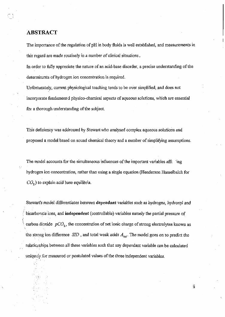
ABSTRACT

The importance of the regulation of pH in body fluids is well established, and measurements in

this regard are made routinely in a number of clinical situations.

In order to fully appreciate the nature of an acid-base disorder, a precise understanding of the

determinants of hydrogen ion concentration is required.

Unfortunately, current physiological teaching tends to be over simplified, and does not

incorporate fundamental physico-chemical aspects of aqueous solutions, which are essential

far a thorough understanding of the subject.

This deficiency was addressed by Stewart who analysed complex aqueous solutions and

proposed a model based on sound chemical theory and a number of simplifying assumptions.

The model accounts for the simultaneous influences of the important variables affc ing

hydrogen ion concentration, rather than using a single equation (Henderson Hasselbalch for

C02) to explain acid base equilibria.

Stewart's model differentiates between dependant variables such as hydrogen, hydroxyl and

bicarbonate ions, and independent (controllable) variables namely the partial pressure of

carbon dioxide pC02, the concentration of net ionic charge of strong electrolytes known as

the strong ion difference SID , and total weak acids Atot. The model goes on to predict the

relationships between all these variables such that any dependant variable can be calculated

uniqutily ib r measured or postulated values of the three independent variables.

To establish whether this model could account for all factors influencing acid-base changes in

a clinical setting it was decided to study patients with Diabetic Ketoacidosis, as the

biochemistry of this disorder is well known. Arterial and venous blood was collected from

twenty patients with the diagnosis of Diabetic Ketoacidosis as part of their routine

management. Hydrogen ion concentrations and the concentrations of the independent variables

were measured, and the results of measured hydrogen concentrations and predicted hydrogen

ion concentrations based on Stewart’s model using measured independent variables were

compared.

/ Extreme discrepancies were found between the measured hydrogen ion concentrations and

those calculated using Stewart's model in this patient group. As the model is able to accurately

predict hydrogen ion concentrations from simple solutions, the reasons for the discrepancies in

complex biological solutions remain uncertain. The two major areas which may account for

these changes are accuracy of measurement and protein chemistry. In conclusion, the sound

chemical and thermodynamic basis of Stewart’s model makes it likely to be correct in

principle, however further research is essential to elucidate the specific causes of discrepancy

between theory and measurement in the clinical setting.

TABLE OF CONTENTS

Page

Acknowledgements................................................................................ i

Abstract.................................................................................................. ii

Introduction and literature review..........................................................1

Summary of the Conventional View of Acid-Base Physiology 2

Review of Stewart’s Model................................................. 6

Aims and Objectives.............................................................................. 26

Subjects...................................... 27

Methods...................................................................... 28

Data Analysis................................................... 29

Results.................................................. .................................................30

Discussion and Conclusion.................................................................... 40

References............................................................................ 45

INTRODUCTION AND LITERATURE REVIEW

Acid-base balance in physiological solutions has been studied for many decades, and while a

number of controversies still exist regarding exaut mechanisms of regulation, there is general

consensus on most aspects of the problem in the orthodox physiological and medical literature.

In fact, much of the theory currently promulgated in acid-base literature was developed in the

1920's and has undergone relatively little change since then.

Unfortunately, all is not well with the conventional view on the subject, and the late 1970's

saw the emergence of a new theory produced by P. A. Stewart, a biophysicist at Brown

University1.

Stewart recognized that the problem of acid-base balance must be analysed in terms of modern

thermodynamic theory of aqueous solutions, and subsequently proceeded to develop a model

which accounts for the theoretical inconsistencies of the currently held views 2.

About one and a half decades have passed since Stewart published his model, and, while there

has been a gradual increase in the number of citations of Stewart's work, there is still no broad

recognition of its validity and applicability. The reasons for this are numerous, however the

most likely are:

1) Stewart’s model is essentially quantitative, and the biological and medical sciences have

until recently been more descriptive, resulting in very few researchers who are able to w M .

the model.

Page 1

2) There is a very vocal core of researchers whose work would be invalidated or at least

require substantial modification if Stewart’s view were to prevail.

3) Experimental validation of Stewart’s model presents a number of intimidating obstacles in

terms of the precision and accuracy required in measuring the determining analytes.

Notwithstanding the above, Stewart’s approach to acid-base balance in physiological solutions

represents the most elegant and theoretically consistent view of the subject to date, and a small

but consistent group of researchers have supported his view.

Summary of the Conventional View of Acid-Base Physiology

The traditional view holds that in the course of normal metabolism approximately 20 000 -

25 OOOmmol of carbonic acid (II2C03) is generated but due to the equilibrium

H2C03 ̂ H 20+C02this acid component is exhaled via the lungs as carbon dioxide, a further

50-100 mmol of H + is produced daily as non-volatile acids as a result of catabolism of

proteins and the incomplete oxidation of carbohydrates and lipids. These non-volatile acids are

normally excreted v'a the kidneys. The kidneys are thought t j play a further role in acid -base

homeostasis by mear. s of the excretion of bicarbonate.

The maintenance of pH within a narrow range is ascribed to buffering. Two mechanisms are

thought to play a major role in this regard. The first is metabolic reactions which preserve

homeostasis by changing their rates in response to acid-base disturbances and in so doing

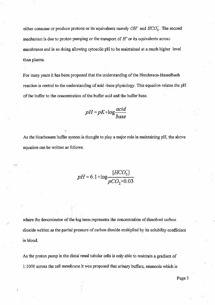
either consume or produce protons or its equivalents namely OH~ and HC02. The second

mechanism is due to proton pumping or the transport of fT or its equivalents across

membranes and in so doing allowing cytosolic pH to be maintained at a much higher level

than plasma.

For many years it has been proposed that the understanding of the Henderson-Hasselbach

reaction is central to the understanding of acid -base physiology. This equation relates the pH

of the buffer to the concentration of the buffer acid and the buffer base.

p H = pK *\og—base

As the bicarbonate buffer system is thought to play a major role in maintaining pH, the above

equation can be written as follows.

p H -6 .1 +log---------------pCO^xQ.OS

where the denominator of the log term represents the concentration of dissolved carbon

dioxide written as the partial pressure of carbon dioxide multiplied by its solubility coefficient

in blood.

As the proton pump in the distal renal tubular cells is only able to maintain a gradient of

1:1000 across the cell membrane it was proposed that urinary buffers, ammonia which is

Page 3

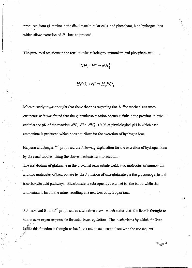
produced from glutamine in the distal renal tubular cells and phosphate, bind hydrogen ions

which allow excretion of H+ ions to proceed.

The presumed reactions in the renal tubules relating to ammonium and phosphate are:

More recently it was thought that these theories regarding the buffer mechanisms were

erroneous as it was found that the glutaminase reaction occurs mainly in the proximal tubule

and that the pK of the reaction JVff3 +iJ+ ̂ A5fJ is 9.03 at physiological pH in which case

ammonium is produced which does not allow for the excretion of hydrogen ions.

Halperin and Jungas3,4,5 proposed the following explanation for the excretion of hydrogen ions

by the renal tubules taking the above mechanisms into account:

The metabolism of glutamine in the proximal renal tubule yields two molecules of ammonium

and two molecules of bicarbonate by the formation of oxo-glutarate via the gluconeogenic and

tricarboxylic acid pathways. Bicarbonate is subsequently returned to the blood while the

ammonium is lost in the urine, resulting in a nett loss of hydrogen ions.

Atkinson and Bourke6,7 proposed an alternative view which states that the liver is thought to

be the main organ responsible for acid -base regulation. The mechanisms by which the liver

fulfills this function is thought to be: 1. via amino acid catabolism with the consequent

/Page 4

production of bicarbonate and ammonium ions and 2. the consumption of bicarbonate during

the ureagenesis cycle.

Ureagenesis would therefore be inhibited in the presence of metabolic acidosis and stimulated

in the presence of a metabolic alkalosis thereby maintaining physiological pH balance.

From the above, it is evident that current physiological acid-base theoiy is inadequate to

account for the complexities of biological solutions.

REVIEW OF STEWART’S MODEL

With the greater availability of computers in the 1970's, it became possible and practical to

deal with a large class of mathematical and physical problems, which had previously proved

too complex for ready manipulation.

It was primarily this factor, combined with his difficulty with the rationale behind the

conventional approach to physiological acid-base balance, that prompted Peter A. Stewart, a

Biophysicist at Brown University, to re-examine the subject of acid-base balance, and to

challenge the conventional viewpoint. His work led to a novel approach to the subject which

is based on modem chemical and thermodynamic principles of solution chemistry1,2.

In order to understand Stewart’s model, it is first necessary to review a few basic aspects of

aqueous solutions which Stewart used as his starting point:

Consider first a hypothetical beaker of absolutely pure water. The aqueous solution contained

therein must consist primarily of molecules of H20 a.s well as some H* and some OH' ions.

Clearly, the origin of the H + and OH' ions is due to the dissociation of water molecules. This

is in fact the only reaction that occurs in pure water, and it must be recognised that this

reaction will proceed to form hydrogen and hydroxyl ions which in turn recombine to form

water molecules at a rate dependant on their concentrations, such that a state of dynamic

equilibrium is reached where the rate of forward reaction equals the rate of the reverse

reaction, and the concentrations of all three species remain constant even though both

reactions continue.

Page 6

h 2o - h ++o h -

The point at which this equilibrium occurs is, in the case of pure water, only dependent on the

temperature, and so the ratio of product to reactant at any given temperature is a constant

which will be called Kw.

K _ m [ O H - ]

It should be mentioned, as pointed out by Stewart, that in accordance with thermodynamic

theory, dissolved species should be described in terms of their thermodynamic activities rather

than their concentrations. However, in dilute solutions, which body fluids can reasonably be

considered to be, there is very little numerical difference in dealing with concentrations as

compared to activities, and for this reason, the more familiar concentration units of

measurement will be used throughout. It must be borne in mind however, that for a more

exact treatment of the subject, activities will have to be retained 8.

Now the central question to be answered is: what determines the hydrogen ion concentration

of this pure water sample at a given temperature?. \

The first step in answering this question is to make a simplifying assumption regarding the

Page 7

water dissociation equation.

The value of Kw, while temperature dependent, is always a very small number, implying that

the concentrations of and OH~ ions are about one thousand million times less than the

concentration of undissociated water molecules. Changes in temperature will cause a change

in the value of Kw and consequently in the concentration of IT (and OH~ ), however even

temperature changes that cause the hydrogen ion concentration to vary 10 fold or even 100

fold for that matter, will hardly change the water concentration from its value which at 37°Cis

about 55.3M.

For this reason, the water concentration can be considered to be constant with negligible loss in

numerical precision. This means that the equation can be simplified by multiplying the

essentially constant concentration of water by Kw to give a new temperature dependent

constant called k 'w, resulting in the following:

< = W W H - ]

This equation is still not sufficient to determine the hydrogen ion concentration for a known

K[9, ie. a graph of hydrogen ion versus hydroxyl ion concentration will produce a hyperbola

which implies an infinite number of possible values for .AT with correspondingly infinite values

fbr'Q #-.

IClearly, a second equation is required to solve for two variables. This is provided by the

Page 8

absolute requirement for electrical neutrality. The solution has no net charge, and thus the

concentration of H* and OH' ions must be identical yielding the second equation ie.

[JT] = [OH'} or [H+] - [OH"] = 0

Clearly, the intersection of the straight line graph produced by the above equation and the

hyperbola produced by the hyperbolic equation yields the solution for hydrogen ion

concentration and hydroxyl ion concentration for this pure water sample. Algebraically, this

can be solved as:

[ f f l = [O IT ] = / <

Note that hydrogen and hydroxyl ion concentrations for pure water are always equal, making

this a neutral solution at all times. The only remaining requirement for determining actual

concentrations, is to know the numerical value of at the temperature under consideration.

At a temperature of 25°C, the value of is 1.01 x 10"14. This implies a hydrogen and

hydroxyl ion concentration of about 10‘7, or a pH of 7,

It is thus clear that at a different temperature (with a different K^), the pH of pure water would

no longer be 7 even though the solution would still ba neutral.

In order to make this pure water solution a little more like a body fluids, one must introduce

strong ions (strong electrolytes). Strong ions are defined as ions which are always in an almost

completely dissociated state in aqueous solution. Examples in physiology include sodium,

potassium and chloride ions. For example, there is almost no NaCl'm solutions but only

Page 9

dissociated Na+ and Cl

The importance of strong ions in terms of acid base behaviour is that they add new terms to the

electrical neutrality equation. As an example, one could imagine an aqueous solution

containing only sodium and chloride (not necessarily in the same concentrations). This again

requires two equations to describe this solution, namely, the equation as before in the pure

water case k!w = [fTjfOfT], and a new electrical neutrality equation incorporating all the ions

ie:

Once again, this electrical neutrality equation implies that the total anion concentration is equal

to the total cation concentration, and real solutions may require that other ions such as

potassium are considered.

For convenience, one may group the difference between the concentrations of strong cations

and strong anions into a single term called the strong ion difference abbreviated [SID] . ie. In

this example let [SID] = [Net+] - [C/ ~]

The two equations describing this system then become:

[ s /£ ] + [ in - [ o /n = o

Page 10

< = [jr ][O jr]

The algebraic solution of the two simultaneous equations is a quadratic equation which can be

solved explicitly for [i7+] and [OH~] as follows:

[ if '] = jKi+(lSIB)l2f-(lSID-\l2)

[OH-] = ^(iSIDy2f*([SlD\l2)

A graphical representation shown below1,12 (in this case at an arbitrary temperature of 44°C) of

these equations shows that when strong cation and strong anion concentrations are equal, the

solution is again neutral and identical to the pure water case (except for a small effect of

osmolality on which can be ignored with very little effect numerically). When the [S'/D]

becomes positive, the OH~ concentration rises sharply while the H + concentration tends

towards zero. The opposite is true for negative [SID] values, where the H' concentration

rises sharply and the OH" concentration tends towards zero. The sodium and chloride ions

can be added to the solution as sodium hydroxide and hydrochloric acid respectively.

Page 11

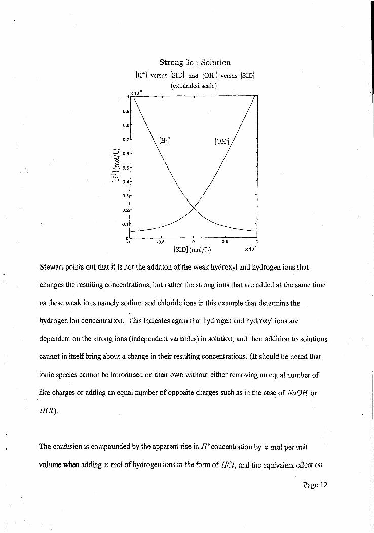
Strong Ion Solution [H+] versus [SID] and [OH'j versus [SID]

(expanded scale)

0.9

0.8

0.7

tf* 0.6

0.5

0.4

0.3

0.2

0.1

0.5- 0.5xIO**[SID] (mol/L)

Stewart points out that it is not the addition of the weak hydroxyl and hydrogen ions that

changes the resulting concentrations, but rather the strong ions that are added at the same time

as these weak ions namely sodium and chloride ions in this example that determine the

hydrogen ion concentration. This indicates again that hydrogen and hydroxyl ions are

dependent on the strong ions (independent variables) in solution, and their addition to solutions

cannot in itself bring about a change in their resulting concentrations. (It should be noted that

ionic species cannot be introduced on their own without either removing an equal number of

like charges or adding an equal number of opposite charges such as in the case of NaOH or

#CZ).

The confusion is compounded by the apparent rise in i f +concentration by x mo! per unit

volume when adding x mol of hydrogen ions in the form of HCl, and the equivalent effect on

Page 12

OH' by adding NaOH, however this apparent one to one correspondence of hydrogen and

hydroxyl ions by the addition of hydrochloric acid and sodium hydroxide respectively is

erroneous. Examination of the quadratic equation for hydrogen ion concentration shows that

the response of the H + concentration becomes very linear against [3ZD] when [«SZD] is very

negative but this correspondence is lost as [SID] approaches to zero. An equivalent effect for

OH' at negative [£/£>] values can be seen by examining the quadratic equation for hydroxyl

ions.

In order to simulate plasma or other body fluids more closely, it is necessary to introduce weak

acids into the system, traditionally classed amongst the so called buffers. Weak acids are

distinguished by their partial dissociation in aqueous solution, in contrast to strong acids such

as HCl which dissociate fully to yield strong ions. Weak acid dissociation can be represented

by the following chemical reaction:

This can be represented quantitatively as:

K _ [H+][A -]" (#4 ]

where Ka represents the dissociation constant for the weak acid under consideration, and is

largely temperature dependent.

Page 13

The most numerically important weak acids in biological solutions are the proteins, while weak

acids such as phosphates are usually present in very small concentrations and can usually be

ignored with very little loss in precision. If one considers the thousands of proteins present in

blood plasma, the problem at first sight appears daunting because a different value for Ka must

be found for each protein. Stewart proposed that in the physiological range of concentrations,

the plasma proteins have Ka values which are sufficiently close to each other, that a single

lumped representative value for Ka can be assumed without much loss in numerical precision.

Even though this procedure may not be strictly valid, it remains a valuable concept in

explaining the model, and additional proteins can always be taken into account as and when

required 9’10’11.

The effect of adding this hypothetical single weak acid in the form of a total protein value is to

introduce an additional anion into the electrical neutrality equation, namely A~, and due to the

new anion, the electrical neutrality equation becomes:

A second mathematical equation results from the physical requirement that the total amount of

weak acid Atot added to the solution must remain constant even though some of the molecules

will be in dissociated form as H* and A \ and some will be undissociated HA. This equation

of conservation of total weak acid is:

Page 14

When the three new equations resulting from weak acid in solution are considered together

with the additional requirement for water dissociation namely K[v = [AT][Off' ], and solved

simultaneously, the result is a third order polynomial in [H+]

[ff = o

The effect of adding a weak acid is to shift the neutrality point to a positive non-zero [57D]

value, ie. The [SID] value at which f f + and OH' concentrations are equal now occurs at a

positive [SZD] value rather than an [SID] of zero as was the case for pure water and aqueous

solutions with strong ions only. In addition to this, the rate of change of [/f+] and [OH~] with

respect to [SID] is greater than in the pure water and strong ion case for the range under

consideration in physiology. This can be seen by inspecting the gradients of the plots of the

resulting equations and comparing them to the strong ion case. This is surprising, when one

considers that buffers are traditionally said to decrease this rate of change. Stewart’s model

shows that this only happens in specific regions of the [SID] range which are usually not of

interest in physiology.

Page 15

Strong Ion - Weak Acid Solution

[H+] versus [SID] and [OH~] versus [SID]

x 10"5

0.9

0.8

0.7

0.3

0.2

0.1

0.030.020.01

[SID] (mol/L)- 0.01

At this point it should be noted that weak bases can be analysed in an equivalent way, however

they are usually not present in physiological solutions in appreciable quantities and can thus

usually be ignored. One example of an exception to this is the presence of the

ammonia/ammonium ion equilibrium in urine in appreciable quantities.

O

One further solute is needed to realistically simulate biological fluids in general and plasma

specifically, namely carbon dioxide. The concentration of C02 is determined by the rate of

metabolism and the rate of elimination by the lungs. C02 concentrations are usually expressed

Page 16

in terms of an equivak it interfacial gas phase partial pressure which would maintain the

dissolved C02 concentration in question at equilibrium. Typically, in healthy human arterial

plasma, C02 is maintained at a partial pressure of about 40mmHg.

There are five chemical reactions that occur in aqueous solution due to the presence of

dissolved C<92, and these are:

C02(aq) + C02(g)

c-OsfogO+

It should be noted that the carbonic anhydrase catalised reacti ,n (abbreviated CA) is normally

a very slow reaction in comparison to the others, and this catalyst has the effect of increasing,

the reaction rate accordingly, and in so doing, results in rapid equilibration of the system which

would otherwise not occur.

It should also be noted that some C02 reacts with groups on protein molecules, however this

reaction, forming carbamino compounds is usually numerically insignificant and will be ignored

in this analysis.

One of the features of C02 reaction in water is the formation of the carbonate ion (C 0 32")

Page 17

which is just as theoretically relevant as bicarbonate but numerically many orders of magnitude

smaller, and is frequently ignored in physiological literature. It should also be noted that

bicarbonate and carbonate ions are dependent variables in the same way as hydrogen and

hydroxyl ions.

The mathematical descriptions of the above chemical reactions relating to C02 are as follows:

[ C O , # ] =

% C O , ] =

[co^ d )] [oar] = [# c o ; ]

The division of the constant by 2 has been introduced12 to correct for the fact that carbonate

(as well as other concentrations) is expressed in mmol/L whereas Stewart used mEq/1 which

resulted in carbonate ion having twice the numerical value due to it being a divalent cation.

It should be noted that by combining variables, the first four equations can be simplified to one

equation ie.

where is must be noted thatZ^ is distinct fromZa , and that the productZyA ^ will be

represented byKc to retain consistency with Stewart12.

The addition of carbon dioxide therefore requires two additional equations to describe the

solution mathematically, where the constant Kc in the second equation is just the appropriate

algebraic combination of constants from the four equations giving rise to it.

The second equation is clearly the non-logarithmic form of the Henderson Hasselbach

equation:

\h c o :\+ logio

^ c o ^ p C O

Page 19

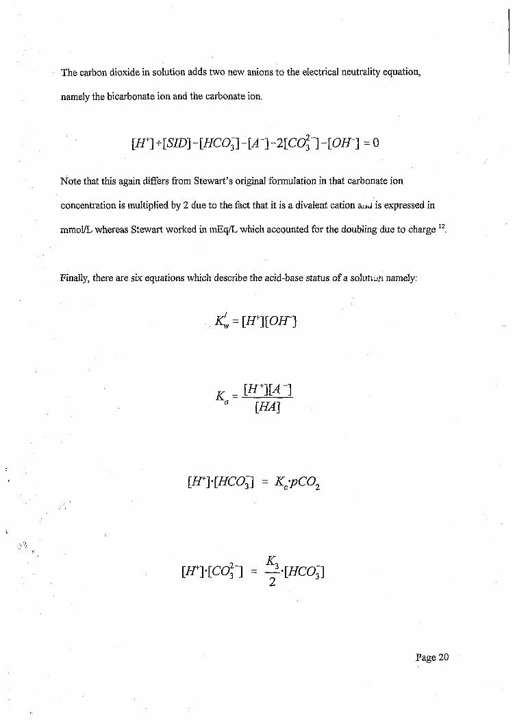
The carbon dioxide in solution adds two new anions to the electrical neutrality equation,

namely the bicarbonate ion and the carbonate ion.

[/r]+[S7D]-[ffC03"]-U']-2[C0 3 ']-[0ff1 =0

Note that this again differs from Stewart’s original formulation in that carbonate ion

concentration is multiplied by 2 due to the fact that it is a divalent cation aw is expressed in

mmoi/L whereas Stewart worked in mEq/L which accounted for the doubling due to charge12.

Finally, there are six equations which describe the acid-base status of a solution namely:

z _

Page 20

mvw] = [Aj

[SID]-[A 1 +[H*MOH~] - [HCO;i-2[COl~] = 0

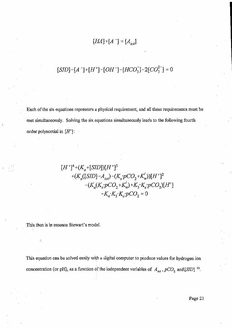
Each of the six equations represents a physical requirement, and all these requirements must be

met simultaneously. Solving the six equations simultaneously leads to the following fourth

order polynomial in [2f+] :

KKa([SID]-AJ-(Kc-pC02+lO )[H '¥ -(Ka{Kc-pC02 +< ) +Ki-K<:pCOJ[ir]

-K;Ki K;pC01 = 0

This then is in essence Stewart’s model.

This equation can be solved easily with a digital computer to produce values for hydrogen ion

concentration (or pH), as a function of the independent variables of A tot, pC02 and[jZD] 13.

Page 21

\H+] is just one of the dependent variables which can be solved for, the others being

bicarbonate ions, carbonate ions, hydroxyl ions, A" ions andi£4 13.

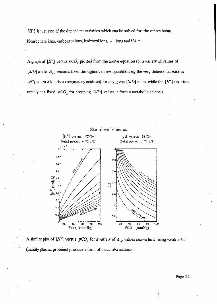
A graph of [iJ+] ver: us pC02 plotted from the above equation for a variety of values of

[<S7D] while Atot remains fixed throughout shows quantitatively the very definite increase in

[ZT] as pC 02 rises (respiratory acidosis) for any given [SID\ value, while the [ i f ] also rises

rapidly at a fixed pC02 for dropping [57Z)j values, a form a metabolic acidosis.

Standard Plasma[H+] versus PCO2

(total protein = 70 g/L)x 10

pH versus PCO2(total protein. ■= 70 g/L)

1.8

1.6

1.4

t o 0.8

0.4

0.2

10060 804020

PCOi (nunHg)

7.8

7.6

7.4%

7.2

6.8

10020 40 60 80

PCO2 (mmHg)

A similar plot of [ZT] versus pC02 for a variety of Aiot values shows how rising weak adds

(mainly plasma proteins) produce a form of metabolic acidosis.

Page 22

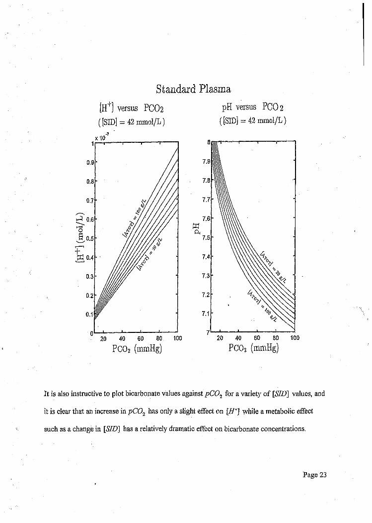
Standard Plasma

[H+] versus PCO2 pH versus PCO2

( [SID] = 42 mmol/L) ( [SID] = 42 mmol/L)

7.9

7.8

7.7

7.6

A7.5

7.4

7.3

7.2

100

0.9

0.8

0.7

0.6r~H

0.2

100

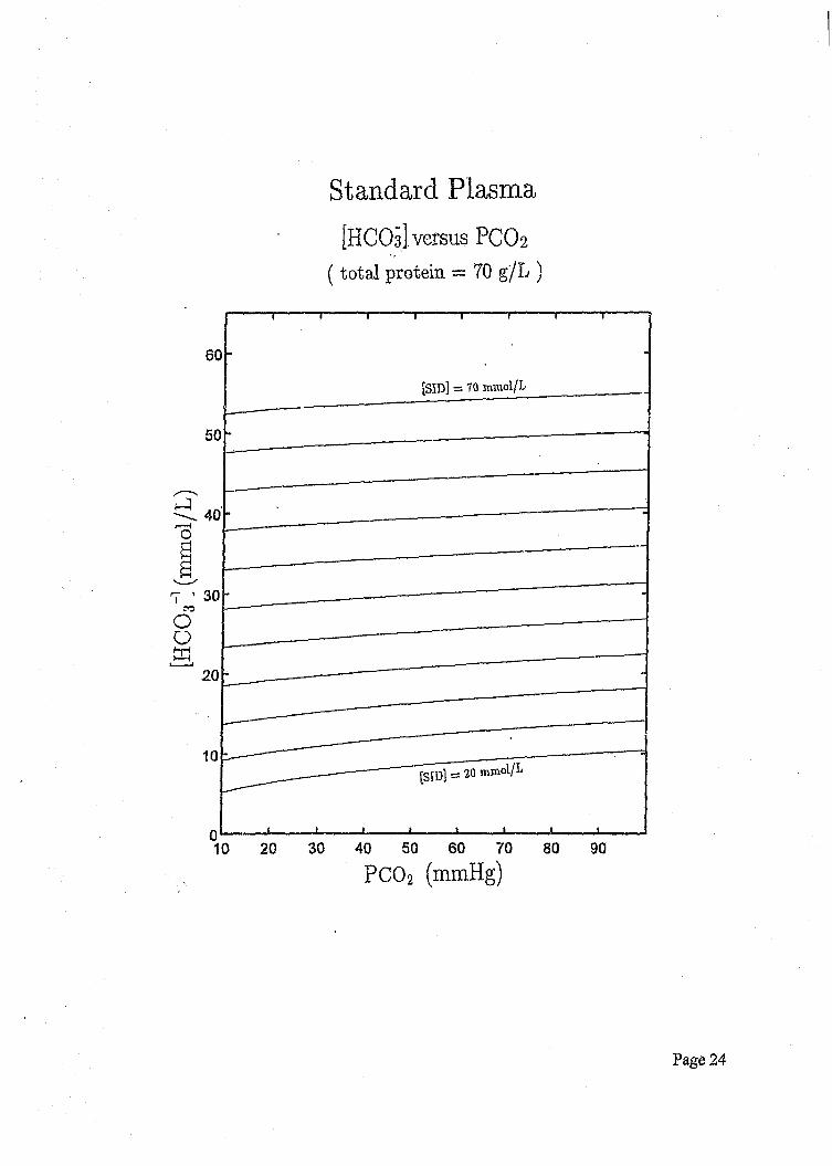
It is also instructive to plot bicarbonate values against pC01 for a variety of [SID] values, and

it is clear that an increase in pC02 has only a slight effect on [ff+] while a metabolic effect

such as a change in [SID] has a relatively dramatic effect on bicarbonate concentrations.

Page 23

[HCO

s ] (r

omol

/L)

Standard Plasma[HCOs] versus PCO 2

( total protein = 70 g/L )

[SID] = 70 mmol/L

Page 24

One of the striking features of Stewart’s model is the fact that with the appropriate values for

the constants, and by using physiologically correct values for the independent variable, the

values for [H+] and other dependent variables produced by the equation are within the

expected range.

In summary, Stewart’s model identifies three independent variables \&.pC02, Atota.nd

[£©] which determine all the other variables including bicarbonate and hydrogen ion

concentration.

It is therefore evident that one cannot postulate a pumping in or out of hydrogen ions or

bicarbonate ions from the plasma compartment as a mechanism to control the final pH value.

There have been a number of reports relating to the obvious advantages of Stewart’s model, as

well as highlighting some of the controversies, while other authors have been severely critical

of this w ork14'15'16.

Other authors have utilised Stewart’s model to analyse various biological solutions 17’18’19’20’21,22,

and there has been a reasonably successful verification of the model in normal subjects23.

Page 25

AIMS AND OBJECTIVES

The objective of this study was to evaluate whether Stewart’s model of acid-base regulation,

which has been shown to be correct in simple solutions, could be applied to a complex clinical

condition namely diabetic ketoacidosis, In addition, the objective of the project was to

highlight any discrepancies between the model’s predictions and clinical measurements in this

common pathological condition, and to try to elucidate obvious sources for any observed

discrepancies.

Diabetic ketoacidosis was chosen to evaluate the behaviour of the model for two reasons:

1) This condition constitutes a group of patients who require urgent venous and arterial blood

sampling for clinical management making it convenient to obtain blood samples.

2) Diabetic ketoacidosis is a well understood clinical entity with well characterised biochemical

changes which could thus be analysed with relative simplicity.

Page 26

SUBJECTS

Arterial and venous blood samples were collected from twenty patients with the diagnosis of

diabetic ketoacidosis. All samples were obtained as part of the routine management of these

patients, at the discretion of the managing doctor. Only patients who were treated with insulin,

fluids and electrolyte replacements were included in the study. Patients known to be on any

other medication were excluded.

Page 27

Methods

Blood for arterial blood gas analysis was collected in commercially prepared heparinised

syringes (Instrumentation Laboratory). Arterial blood gas analysis was performed immediately

following collection, by means of ion selective electrodes (ISE) at 37 degrees centigrade on

the IL 1306 blood gas analyser (ILEX). The blood gas analyser was calibrated and three

levels of controls were run before each specimen was analysed.

Venous blood for electrolytes, ketones and protein analyses was collected in normal clotted

tubes while blood for lactate and glucose analyses was collected in fluoride tubes. Blood was

centrifuged at 3500 rpm for 10 minutes. Aliquots of blood were immediately analysed and

used for clinical management while duplicates were stored at -70° C and analysed as a batch at

a later time to exclude inter-batch variation, for the purposes of the project, Electrolytes

(ISE), total proteins (Biuret) and albumin (Bromocresol-green) were analysed on the Hitachi

747 autoanalyser (Boehringer Mannheim). The 747 autoanalyser was calibrated and controls

(PPU and PNU, Boehringer Mannheim) at two levels were used to determine the accuracy of

analysis. Precision of analysis was determined using Monotrol control material at two

separate levels. Lactate was measured on the TDX (lactate dehydrogenase, Abbott

Diagnostics), three different levels of control material (Abbott) was used to determine the

accuracy of the test prior to analysing the specimens. Ketones were analysed on the Cobas

mira using the Randox Rambut kit. Randox control material at two different levels was used

to determine the accuracy of the aceto- acetate kit. As no quality control material for Beta-

hydroxybutyrate was commercially available, control material was made up adding a known

quantity of Betahydroxybutyrate (Sigma Chemicals) to laboratory grade water.

Page 28

DATA ANALYSIS

The relationship between the measured hydrogen ion concentration and that calculated using

Stewart’s model, was analysed by means of a simple regression analysis. It is self evident that

perfect agreement would constitute a 45 degree regression line of identity.

In addition to this, techniques of error analysis were used, whereby expected random error

was calculated for over a wide range of measurements based on the known variability

established from repeated measurements on control material The actual percentage errors of

the calculated results with respect to measured hydrogen ion concentrations were determined

and compared.

Page 29

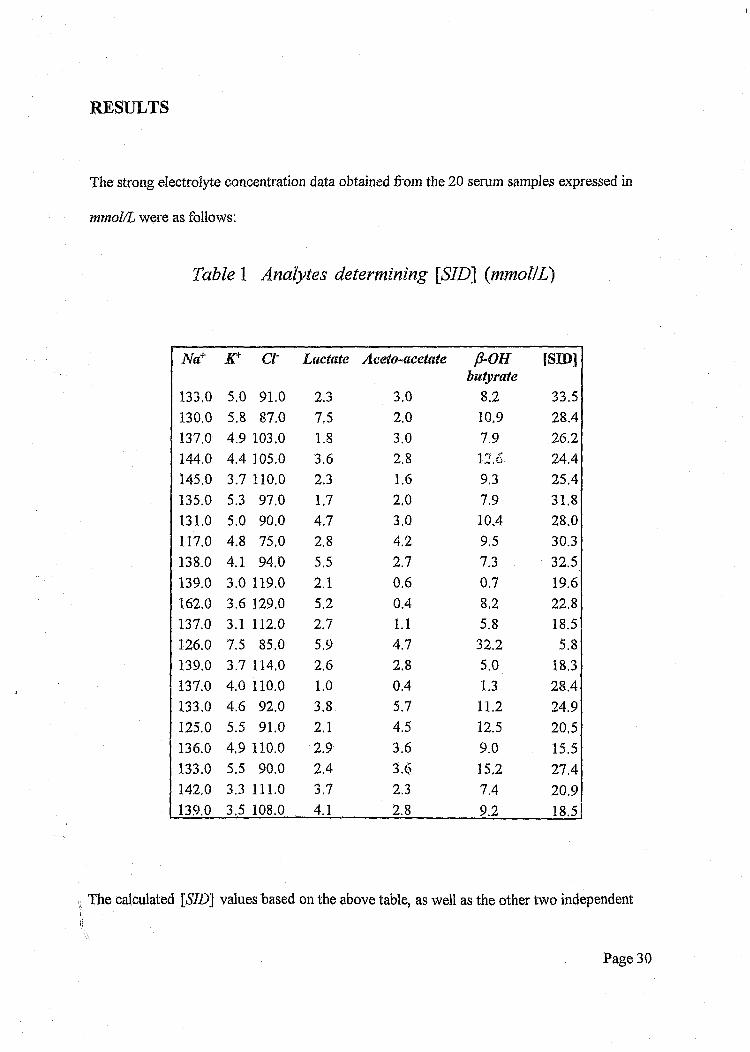
RESULTS

The strong electrolyte concentration data obtained from the 20 serum samples expressed in

mmol/L were as follows:

Table 1 Analytes determining [STD] {mmol/L)

Na+ Cl Lactate Aceto-acetate p-OHbutyrate

[SID]

133.0 5.0 91.0 2.3 3.0 8.2 33.5130.0 5.8 87.0 7.5 2.0 10.9 28.4137.0 4.9 103.0 1.8 3.0 7.9 26.2144.0 4.4 105.0 3.6 2.8 12.6 24.4145.0 3.7 110.0 2.3 1.6 9.3 25.4135.0 5.3 97.0 1,7 2.0 7.9 31.8131.0 5.0 90.0 4,7 3.0 10.4 28.0117.0 4.8 75.0 2.8 4.2 9.5 30.3138.0 4.1 94.0 5.5 2.7 7.3 32.5139.0 3.0 119.0 2.1 0.6 0.7 19.6162.0 3.6 129.0 5.2 0.4 8.2 22.8137.0 3.1 112.0 2.7 1.1 5.8 18.5126.0 7.5 85.0 5.9 4.7 32.2 5.8139.0 3.7 114.0 2.6 2.8 5.0 18.3137.0 4.0 110.0 1.0 0.4 1.3 28.4133.0 4.6 92.0 3.8 5.7 11.2 24.9125.0 5.5 91.0 2.1 4.5 12.5 20,5136.0 4,9 110.0 2.9 3.6 9.0 15.5133.0 5,5 90.0 2.4 3.6 15.2 27.4142,0 3.3 111.0 3.7 2.3 7.4 209139.0 3.5 108.0 4.1 2.8 9.2 18.5

The calculated [«S7Z>] values based on the above table, as well as the other two independent

Page 30

variables viz. pC02 and total protein Atot are presented below:

Table 2 Independant variables

pCOj ^tot [SID]minHg mmoI/L12.2 57.0 33.524.0 67.0 28.414.8 63.0 26.227.4 46.0 24.411.7 82.0 25.422.8 79.0 31.816.1 74.0 28.029.3 59.0 30.327.2 76.0 32.525.9 49.0 19.631.0 78.0 22.819.4 57.0 18.512.5 71.0 5.821.4 58.0 18.323.5 58.0 28.412.2 80.0 24.912.4 83.0 20.512.6 65.0 15.523.9 84.0 27.412.8 57.0 20.913.2 73.0 18.5

From this data, predicted hydrogen ion concentrations were calculated using Stewart’s model

by utilising a BASIC computer program specifically written for this analysis and based on an

Page 31

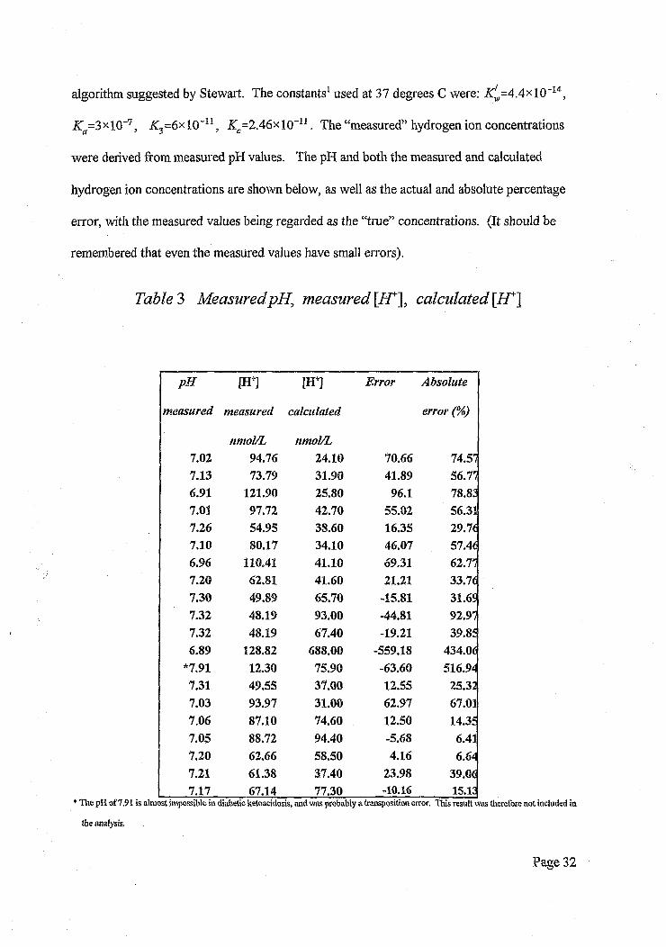
algorithm suggested by Stewart. The constants1 used at 37 degrees C were: ^ = 4 .4 x l0 -14,

Ka=3xl0~7, K3=6xl0~u , Zc=2 .4 6 x l0 "11. The “measured” hydrogen ion concentrations

were derived from measured pH values. The pH and both the measured and calculated

hydrogen ion concentrations are shown below, as well as the actual and absolute percentage

error, with the measured values being regarded as the “true” concentrations. (It should be

remembered that even the measured values have small errors).

Table 3 Measured pH, measured [AT], calculated [H*~\

pH m m Error Absolute

measured measured calculated error (%)

nmol/L nmol/L7.02 94.76 24.10 70.66 74.577.13 73.79 31.90 41.89 56.776.91 121.90 25.80 96.1 78.837.01 97.72 42.70 55.02 56.317.26 54.95 38.60 16.35 29.767.10 80.17 34.10 46.07 57.466.96 110.41 41.10 69.31 62.777.20 62.81 41.60 21.21 33.767.30 49.89 65.70 -15.81 31.6$7.32 48.19 93.00 -44.81 92.977.32 48.19 67.40 -19.21 39.856.89 128.82 688.00 -559.18 434.06

*7.91 12.30 75.90 -63.60 516.947.31 49.55 37.00 12.55 25.327.03 93.97 31.00 62.97 67.017.06 87.10 74.60 12.50 14.357.05 88.72 94.40 -5.68 6.417,20 62.66 58.50 4.16 6.647.21 61.38 37.40 23.98 39.067.17 67.14 77.30 -10.16 15.13

* The pH of 7.91 is almost impossible in diabetic ketoacidosis, and was probably a transposition error. This result was therefore not included in

the analysis.

Page 32

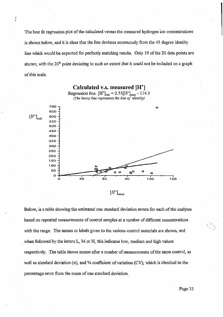
The best fit regression plot of the calculated versus the measured hydrogen ion concentrations

is shown below, and it is clear that the line deviates enormously from the 45 degree identity

line which would be expected for perfectly matching results. Only 19 of the 20 data points are

shown, with the 20th point deviating to such an extent that it could not be included on a graph

of this scale.

Calculated v s. measured [H+]Regression line: [H+]calc = 2.55[H+]meils -114.3

(Fhe heavy line represents the line o f identity)

700650

600'calc

550500

450400

350

300

250

200 1 50

TOO

50

O 30 60 90 1 50120

fiTlL Jmeas

Below, is a table showing the estimated one standard deviation errors for each of the analytes

based on repeated measurements of control samples at a number of different concentrations

with the range. The names or labels given to the various control materials are shown, and

when followed by the letters L, M or H, this indicates low, medium and high values

respectively. The table shows means after a number of measurements of the same control, as

well as standard deviation (o), and % coefficient of variation (CV), which is identical to the

percentage error from the mean of one standard deviation.

Page 33

Table 4 Estimated analyte errors

Analyte Control mean a c r

Sodium ion Na monl 134.5 1.5 1.13(mmol/L) Na mon2 112.7 1.2 1.07

Na PNU 116.1 2.9 2.51NaPPU 136.7 2.8 2.06

Potassium ion K monl 6.45 0.1 1.63{mmol/L) KmonZ 4.35 0.05 1.26

K PNU 4.5 0.12 2.57KPPD 6.19 0.15 2.37

Chloride ion CL monl 99.6 1.9 1.96(mmol/L) CL mon2 91 2 2.2

CL PNU 88.3 2.1 2.33CL PPT- 107.4 2.4 2.21

Total Proteins TP monl 74.7 2 2.63TP mon2 43.3 1.2 2.79TP PNU 52.1 0.9 1.76TPPPU 48.6 1.6 3.3

B-OH butyrateBHYD 1 302.8 8.5 2.8(fimol/L) BHYD 2 1148.6 34.3 3

Aceto-acetate A cetL 111.56 5.72 5.13(fimol/L) AcetM 222.22 14.02 6.3

AcetH 564.22 14.66 2.6Lactate Lact L 2.23 0.09 4.05(mmol/L) LactM 5.11 0.09 1.76

LactH 10.25 0.17 1.66pC 02 pCQ2L 21.86 0.52 2.37

(mmHg) pC 02M 36.68 0.7 1.9pCOz H 61.71 1.32 2.14

Hydrogen ion H L 24.81 0.23 0.93(nmol/L) H M 38.13 0.53 1.39

H E 67.7 1.03 1.52

The error analysis performed on Stewart’s model is as follows:

Experimental data are always subject to some error, and interpretation of results must always

take this factor into account.

Broadly speaking, there are two types of error that can occur in experimentation viz. random

error and systematic error.

Random error refers to random fluctuation in the measurement about the “true” value. This

“true” value can be estimated by the mean of multiple readings of the same data. One

important characteristic of random error is that it has a Normal or Gaussian distribution about

the mean value, and the distribution can be fully characterised by the mean and standard

deviation. The presence of random error gives rise to the finite precision of a measurement,

which can be improved by attention to the experimental technique and by averaging multiple .

readings.

Systematic error applies to a fixed or well characterised deviation of the measurement from

the “true” value, and gives rise to the finite accuracy of a measurement. This can be corrected

for by calibration against a standard measure.

The data measured in this project was calibrated by the use of standards to produce calibration

curves which were internally generated in most of the instrumentation. It is therefore

expected that systematic error will play a small role in the overall error.

Page 35

More importantly, random error must be well characterised and accounted for.

Controls for each of the analytes were measured a number of times to establish mean and

standard deviations, and in so doing, to characterise the error in the individual measurements.

For the remainder of this discussion, the error in any measurement will refe. ' o one standard

deviation generally expressed as a percentage of the mean.

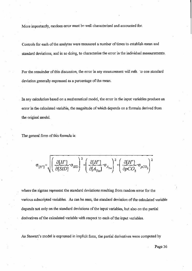
In any calculation based on a mathematical model, the error in the input variables produce an

error in the calculated variable, the magnitude of which depends on a formula derived from

the original model.

The general form of this formula is:

PH"d m ,

\ 2 /

•aSID +s [a t J

+ ap C 0 2

where the sigmas represent the standard deviations resulting from random error for the

various subscripted variables. As can be seen, the standard deviation of the calculated variable

depends not only on the standard deviations of the input variables, but also on the partial

derivatives of the calculated variable with respect to each of the input variables.

As Stewart’s model is expressed in implicit form, the partial derivatives were computed by

Page 36

implicit differentiation and then solved for in each case.

The solutions for the partial derivatives are as follows12:

am _ cm^Kjccm*K,Kcm*Kjc,K dpC02 V

dm -vrf-KaVrf'[S/D] V

a[/r] ^ m 2v

where:

V = 4[iJ+]3 +3Za [ / /+]2 +3 [57D] [H\2 +2KJSID] [H+]

- 2 K /TJW ]-2KcpC02m - 2 K ,JiH*]-Kj:cpC02-K X -K ,K cpC02

The [STD] itself is subject to error, however as it is simply computed by taking the sums and

differences of the various electrolyte charge concentrations, the partial derivatives in the error

formula are unity, and the error equation reduces to being square root of the sum of the

squares of the one standard deviation values for each of the analytes.

Page 37

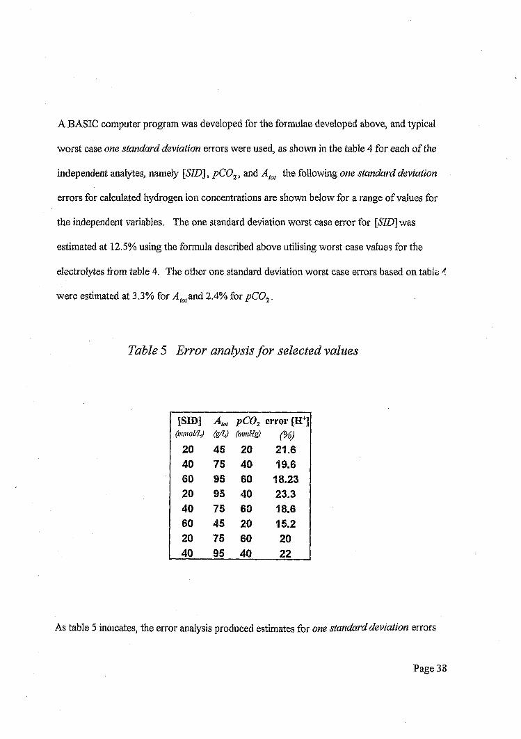
A BASIC computer program was developed for the formulae developed above, and typical

worst case one standard deviation errors were used, as shown in the table 4 for each of the

independent analytes, namely [SID], pC02, and Atot the following one standard deviation

errors for calculated hydrogen ion concentrations are shown below for a range of values for

the independent variables. The one standard deviation worst case error for [S7D] was

estimated at 12.5% using the formula described above utilising worst case values for the

electrolytes from table 4. The other one standard deviation worst case errors based on table 4

were estimated at 3.3% for v4to(an d 2.4% for pC02.

Table 5 Error analysis fo r selected values

[SID] ^ to t 1 3

{mmol/LJ w (mmHg)

20 45 20 21.640 75 40 19.660 95 80 18.2320 95 40 23.340 75 60 18.660 45 20 15.220 75 60 2040 95 40 22

As table 5 indicates, the error analysis produced estimates for one standard deviation errors

Page 38

with respect to the “true” concentration of hydrogen ions varying between about 15% and

23%

Clearly the errors obtained from the analysis as presented in table 3 are much greater than

those predicted by the random error analysis, with only 4 out of the 20 percentage errors

falling within one standard deviation of the expected value.

Page 39

DISCUSSION AND CONCLUSION

The very elegant model proposed by Stewart to explain acid-base physiology and the

numerous factors involved in its control is a great stride forward into research of this most

complex and important field.

From the data presented however it is clear that the percentage errors obtained from using

Stewart's model to calculate hydrogen ion concentration are far in excess of those predicted

based purely on an analysis of the random errors,

In order to begin to achieve an understanding of the discrepancies, a number of possibilities

should be explored.

It has been mentioned that Stewart was well aware of some of the simplifying assumptions

that he made in developing this model, and it is very possible that some of these factors could

contribute greatly to the errors. However, in view of the relative thermodynamic rigour which

Stewart brought to bear on his analysis, and his strict adherence to sound principles of physical

chemistry, it is highly unlikely that the entire model is incorrect, but rather that if any changes

are required, they are likely to relate to detail and non-linearities in coefficients.

Unaccounted for substances remain a strong possibility for the source of error, and can be

divided into two categories.

Page 40

1) Those substances which are well known but are considered to exist in low enough

concentrations as to be numerically insignificant.

2) Substances such as medications and metabolic products which are not known to exist in the

sera under examination or have not been measured.

The first group, ie. those substances regarded as being numerically insignificant, would include

substances such as calcium, magnesium, phosphates and sulfates. In general, these substances

would be found in ionic concentrations less than about 2 or 3 mmol/L, although in terms of

ionic contribution this must be doubled to accommodate the effects of divalent cations and

anions. It must also be borne in mind that phosphates are weak ions, and as such they do not

contribute as dominantly as the other strong ions. Furthermore the positive and negative ions

would at least to some extent cancel out their effect.

Nonetheless, the possibility remains that one or more of these substances may exist in

concentrations where the usual assumptions of insignificance no longer applies.

The second group of substances ie. the unknown group, would include medications and their

metabolites, of which the staff are unaware, or even substance such as non-conventional or

alternative medications. These substances may well exist in the se. '< f some patients and

would be very difficult and in some cases impossible to identify and quantify without the

benefit of a correct history and sophisticated methodologies.

The possible influence of plasma proteins on the model is perhaps the most difficult to

Page 41

quantify, and may in fact be the very area in which the model needs modification.

Firstly, Stewart’s assumption of a representative equilibrium constant for all plasma proteins

may well be a serious oversimplification of reality. The constant may in fact prove to be highly

non-linear due to a possible dependence of the equilibrium constant on hydrogen ion

concentration itself, or perhaps even on other ionic species. This will only be determined by

extensive experimentation.

Secondly, while some workers appear to have demonstrated that proteins may have complex

effects25, and that it is only albumin 10 which determines the acid-base effects of plasma

proteins, this may in fact also be an oversimplification, and furthermore, even if this is correct,

it would imply a requirement to first determine the albumin to globulin ratio and then apply a

conection factor to the total protein values used in this study. Other workers have

demonstrated that the equilibrium constant of protein depends in a rather complex way on the

specific proteins structure and functional groups10.

Thirdly, it is not at all impossible that factors as yet not considered may affect the behaviour of

proteins. A possible example of this is the undetermined effect of glycation. It is well known

that persistently high glucose levels encountered in diabetics produce glycation of various

proteins. It is therefore not at all impossible that glycation may have an important effect on

the equilibrium constants of plasma proteins, something which again will only be determined

by further experimental research.

Finally, the important possibility of measurement errors needs to be considered as a cause for

Page 42

discrepant results.

The first possibility for erroneous measurements is that of the partial pressure of carbon

dioxide. While the random error for the controls used for carbon dioxide measurements are

very acceptable, and would not contribute substantially to the error, it must be recognised that

control samples were not available for the very low carbon dioxide levels encountered in keto-

acidotic patients, and it may well be true that the error at this part of the range is unacceptably

high. It should also be recognised, that in the absence of adequate standard and control

material, not only is it impossible to characterize the random error, but also the possibility of

systematic error due to non-linearity at the extremes of the range cannot be excluded.

The keto-acid P-hydroxy butyric acid measurements depended on controls and standards that

were not well characterised at the levels under consideration. The standards and control

materials for P-hydroxy butyric acid were available for levels far lower than those encountered

in typical keto-acidotic sera, and for this reason, as in the case of carbon dioxide, it is not

possible to draw definitive conclusions regarding systematic and random errors.

The aceto-acetate controls and standards were prepared in-house as commercially available

assayed control material was unobtainable. Crystaline aceto-acetic acid was used to prepare

control material. While this had the advantage of being able to achieve concentrations at any

point in the anticipated range, the technique suffered from the disadvantage of not having an

external assay system for calibration and control.

Page 43

It is clear from the above discussion that there are numerous factors which have not been

adequately accounted for, and that any one or more of these may produce gross errors in the

predicted results.

Notwithstanding the above, Stewart’s model provides an elegant explanation of the observed

behaviour of hydrogen ions in physiological solutions In view of considerations of modem

thermodynamic theory and physical chemistry, there can be little doubt that the model is

correct in principle, and what remains is to reduce the simplifications to the point that the

model accurately reflects conditions in physiological solutions.

It is thus clear that in order to validate the model and to possibly introduce modifications

which correct for some of the oversimplifications, extensive and precise experimental work

remains to be performed. However, it is doubtful if the routine chemical pathology laboratory

can provide adequate analytical precision to achieve this goal.

Furthermore, even when the model is fully validated and adequately modified to reflect the

complexity of biological solutions, it remains questionable as to whether the coarse precission

and accuracy typically required for most medical decision making will be adequate to allow for

the clinical use of the model. Nonetheless, Stewart’s approach must surely be regarded as a

high point in the understanding of an important physical and physiological process.

Page 44

REFERENCES

1. Stewart PA. How to understand acid-base. Elsevier Press. 1981; 1-181.

2. Stewart PA. Modern quantitative acid-base chemistry,. Can. J.Physiol. Phcmacol. 61: 1444-1461.

3. Halperin ML. How much ‘new’ bicarbonate is formed in the distal nephron in the process of net acid excretion. Kidney Int. 1989;35: 1277-1281.

4. Halperin ML, Jungas RLL. Metabolic production and renal disposal of hydrogen ions. Kidney Int. 1983; 24 :709-713.

5. Halperin ML, Jungas RLL, Cheema-Dhadi S, Brosman JT. Disposal of the daily acid load: an integrated function of the liver, lungs and kidney. TIBS. 1987;12:197-199.

6. Atkinson DE, Bourke E. The role of ureagenesis in pH homeostasis. .TIBS. 1984;9:297-3130.

7. Atkinson DE, Bourke E. Metabolic aspects of the regulation of systemic pH. Ain J Physiol. 1987; 252: F987-F956.

8. Robinson RA, Stokes RH. Electrolytic solutions. 1959 2nd ed. Butterworths, Scientific Publications. London.

9. Rossing TH, Maffeo N, Fend V. Acid base effects of altering plasma protein concentrations in human blood. JApplPhysiol.\9%6\ 61:2260-2265.

10. Figge J, Mydosh T, Fend V. The role of serum proteins in acid-base equilibria. J Lab Clin Med\991; 117: 453-467.

11. Figge J, Mydosh T, Fend V. Serum proteins and acid-base equilibria: a follow-up. J Lab Clin Med 1992; 120: 713-719.

12. D. M. Rubin - unpublished work.

13. Stewart PA. Independent and dependent variables of acid-base control. Respir. Physiol. 1978; 33:9-26.

14. Cameron JN. Acid-base homeostasis: past and present perspectives. Physiological Zoology. 1989; 62(4): 845-865.

15. Reeves RB. Commentary on the review article by Dr Peter Stewart.CanJ.Physiol.Pharmacol. 1983:61:1442-1443.

16. Siggaard-Andersen O, Fogh-Andersen N. Base excess or buffer base (strong ion difference) as a measure of a non-respiratory acid-base disturbance. Acta Anaesthesiol Scand. 1995; 39 (sup 107): 123-128.17. Kowalchuk JM, Heigenhauser GIF, Lindinger MI, Sutton JR, Tones ML. Factors influencing hydrogen ion concentration in muscle after intense exercise. JApplPhysiol.19%%', 65:2080-2089.

18. Kowalchuk JM, Heigenhauser GJF, Lindinger MI, Obminski G, Sutton JR, Jones NL. Role of lungs and inactive muscle in acid base control after maximal exercise. JAppl Physiol. 1988; 65:2090-2096.

19. Lindinger MI, Heigenhauser GJF, Spriet HL. Effects of intense swimming and tetanic electrical stimulation on skeletal muscle ion and metabolites. J.Appl. Physiol. 1987; 63:2331-2339.

20. Siainsby WN, Eitzman PD. Role of C02, 02 and acid in arteriovenous [H+] differences during muscle contractions. J.Appl Physiol. 65(4): 1803-1810.

21. Alfaro V, Peinado VI, Palacios L. Factors influencing acid-base status during acute severe hypothermia, in unanesthetized rats. Resp Physiol. 1995: 100: 139-149.

22. Jennings D. The physiochemistry of [H+] and respiratory control: roles of pC02 strong ions and their hormonal regulators. Can J Physiol Pharmacol. 1994; 72: 1499-1512.

23. Weinstein Y, Magazanik A, Grodjinovsky, Inbar O, DlinRA, Stewart PA. Re-examination of Stewarts quantitative analysis of acid-base status. MedSci Sports Exerc. 1991; 23: 1270-1275.

24. Taylor JR. An introduction to error analysis. The study of uncertainties in physical measurement.. Second edition. 1997. University Science Books.

Page 46

Author Paiker J E

Name of thesis Evaluation Of Stewart'S Model For Acid-Base Balance In Patients With Diabetic Ketoacidosis Paiker J E 1999

PUBLISHER: University of the Witwatersrand, Johannesburg

©2013

LEGAL NOTICES:

Copyright Notice: All materials on the Un i ve r s i t y o f the Wi twa te r s rand , Johannesbu rg L ib ra ry website are protected by South African copyright law and may not be distributed, transmitted, displayed, or otherwise published in any format, without the prior written permission of the copyright owner.

Disclaimer and Terms of Use: Provided that you maintain all copyright and other notices contained therein, you may download material (one machine readable copy and one print copy per page) for your personal and/or educational non-commercial use only.

The University of the Witwatersrand, Johannesburg, is not responsible for any errors or omissions and excludes any and all liability for any errors in or omissions from the information on the Library website.