Evaluation of the updated YSU planetary boundary layer

Evaluation of the updated YSU planetary boundary layer schemewithin WRF for wind resource and air quality assessments

Xiao-Ming Hu,1 Petra M. Klein,1,2 and Ming Xue1,2

Received 12 March 2013; revised 5 September 2013; accepted 8 September 2013; published 24 September 2013.

[1] In previous studies, the Yonsei University (YSU) planetary boundary layer (PBL)scheme implemented in the Weather Research and Forecasting (WRF) model was reportedto perform less well at night, while performing better during the day. Compared toobservations, predicted nocturnal low-level jets (LLJs) were typically weaker and higher.Also, the WRF model with Chemistry (WRF/Chem) with the YSU scheme was reported tosometimes overestimate near-surface ozone (O3) concentration during the nighttime. Theupdates incorporated in WRF version 3.4.1, include modifications of the nighttime velocityscale used in the YSU boundary layer scheme. The impacts of this update on the predictionof nighttime boundary layers and related implications for wind resource assessment and airquality simulations are examined in this study. The WRF/Chem model with the updatedYSU scheme predicts smaller eddy diffusivities in the nighttime boundary layer, andconsequently lower and stronger LLJs over a domain focusing on the southern Great Plainsarea, showing a better agreement with the observations. As a result, related overestimationproblems for near-surface temperature and wind speeds appear to be resolved, and thenighttime minimum near-surface O3 concentrations are better captured. Simulated verticaldistributions of meteorological and chemical variables for weak wind regimes (e.g., in theabsence of LLJ) are less impacted by the YSU updates.

Citation: Hu, X.-M., P. M. Klein, and M. Xue (2013), Evaluation of the updated YSU planetary boundary layer schemewithinWRF for wind resource and air quality assessments, J. Geophys. Res. Atmos., 118, 10,490–10,505, doi:10.1002/jgrd.50823.

1. Introduction

[2] Accurate simulations and forecasts of boundary layerwinds are important for the wind power industry [Stormand Basu, 2010; Carvalho et al., 2012], agriculture sectors[Prabha and Hoogenboom, 2008; Prabha et al., 2011], andair quality management [Bao et al., 2008; Cheng et al.,2012; Gilliam et al., 2012]. Planetary boundary layer (PBL)parameterization schemes are of vital importance for accuratesimulations of wind, turbulence, and air quality in the loweratmosphere and thus play an important role for a number ofapplications [Steeneveld et al., 2008; Storm et al., 2009;Carvalho et al., 2012; Hu et al., 2012; García-Díez et al.,2013]. PBL parameterization schemes have been steadilyimproved over the past few decades. However, errors anduncertainties associated with PBL schemes still remain one ofthe primary sources of inaccuracies of model simulations[Zhang and Zheng, 2004; Pleim, 2007a, 2007b; Teixeiraet al., 2008; Hu et al., 2010a, 2010b, 2012; Nielsen-Gammon

et al., 2010]. While much progress has been made in simulatingdaytime convective boundary layer (CBL), progress with themodeling of nighttime boundary layer has been slower[Salmond and McKendry, 2005; Beare et al., 2006; Brownet al., 2008; Hong, 2010] and systematic overestimations ofnear-surface winds during stable conditions have been noticedin the simulations with several meteorological models [e.g.,Zhang and Zheng, 2004; Miao et al., 2008; Han et al., 2008;Shimada et al., 2011; Vautard et al., 2012; Garcia-Menendezet al., 2013; Zhang et al., 2013; Wolff and Harrold, 2013].[3] A few recent studies examined the sensitivity of the

Weather Research and Forecasting (WRF) [Skamarocket al., 2008] model predictions to PBL schemes [Jankov et al.,2005, 2007; Li and Pu, 2008; Borge et al., 2008; Hu et al.,2010a, 2012; Gilliam and Pleim, 2010; Mohan and Bhati,2011; Xie et al., 2012, 2013; Floors et al., 2013; Sterket al., 2013; Yang et al., 2013; Coniglio et al., 2013; Yveret al., 2013]. The performance of different PBL schemesvaries depending on the meteorological conditions, e.g.,nonlocal PBL schemes were reported to perform better thanlocal PBL schemes in the daytime CBL. However, Shin andHong [2011] discuss that excessive daytime mixing, simu-lated by some nonlocal PBL schemes, may also lead tooverly mixed vertical profiles in the residual layer. In gen-eral, local PBL schemes appear to provide a more realisticrepresentation of the nighttime boundary layer [Hu et al.,2010a; Shin and Hong, 2011; Svensson et al., 2011; Kollinget al., 2012; LeMone et al., 2013], but further improvementof PBL schemes, especially for nighttime boundary layer, is

1Center for Analysis and Prediction of Storms, University of Oklahoma,Norman, Oklahoma, USA.

2School of Meteorology, University of Oklahoma, Norman, Oklahoma,USA.

Corresponding author: X.-M. Hu, Center for Analysis and Predictionof Storms, University of Oklahoma, Norman, Oklahoma 73072, USA.([email protected])

©2013. American Geophysical Union. All Rights Reserved.2169-897X/13/10.1002/jgrd.50823

10,490

JOURNAL OF GEOPHYSICAL RESEARCH: ATMOSPHERES, VOL. 118, 10,490–10,505, doi:10.1002/jgrd.50823, 2013

urgently warranted [Hanna and Yang, 2001; Zilitinkevichet al., 2007; Teixeira et al., 2008; Grisogono and Belusic,2008; Fernando and Weil, 2010; Grisogono, 2010; Lareauet al., 2013; Sterk et al., 2013].[4] Most evaluation and improvement work of air quality

models focused on peak ozone (O3) values during the day-time (i.e., the maximum 1 h or maximum 8 h running averageO3 mixing ratios). As a result, some models are overtuned toachieve acceptable model-to-data error statistics in termsof maximum 1 h or maximum 8 h average O3, while they per-form less well for periods with lower O3 concentrations (e.g.,nighttime, Arnold and Dennis, 2001; Mebust et al., 2003;Hu, 2008; Stockwell et al., 2013). Overestimation of nighttimesurface O3 is a common problem for many air quality models[Mao et al., 2006; Chen et al., 2006; Chen et al., 2008;Engardt, 2008; Zhang et al., 2009; Lin and McElroy, 2010;Hu et al., 2010c; Žabkar et al., 2011]. Such overestimationof nighttime surface O3 is speculated to be partially due toincorrect model representation of the PBL [Eder et al.,2006; Herwehe et al., 2011; Žabkar et al., 2011], underesti-mation of O3 dry deposition [Mao et al., 2006; Chen et al.,2006; Chen et al., 2008; Zhang et al., 2009; Lin andMcElroy, 2010], and/or uncertainties in emissions [Žabkaret al., 2011]. In this study we will examine the impact of ver-tical mixing treatment on the prediction of nighttime bound-ary layer structure and O3 concentration.[5] The Yonsei University (YSU) [Hong et al., 2006;

Hong, 2010] PBL scheme is a first-order nonlocal scheme,with a countergradient term and an explicit entrainment termin the turbulence flux equation. It has been widely used inmeteorological and atmospheric chemistry simulations. TheWRF model with the YSU PBL scheme appears to realisti-cally capture the vertical structure of meteorological andchemical variables during the daytime, while it has beenshown to have larger biases during nighttime [Storm et al.,2009; Hu et al., 2012]. Simulations with WRF versions 2.1,2.2, and 3.1.1 using the YSU scheme are found to severely un-derestimate the nighttime wind speed shear exponent [Stormand Basu, 2010]. Other studies [e.g., Storm et al., 2009; Shinand Hong, 2011; Deppe, 2011; Hu et al., 2012; Schumacheret al., 2013; Draxl et al., 2012; Floors et al., 2013] alsoreported that WRF (versions 2.2, 3.1, 3.1.1, 3.2, 3.2.1, and3.4) with the YSU scheme tends to destroy the boundary layervertical wind gradient during nighttime. As it turned out, such

large nighttime biases in all versions between 3.0 and 3.4 ofthe WRF model were at least partially due to excessivelystrong mixing during nighttime that can be attributed to acoding bug in the YSU scheme implemented in the early ver-sions ofWRF. This bug has been fixed inWRF version 3.4.1.One of the goals of this paper is to document the impact ofthis bug fix on the prediction of boundary layer meteorologyand O3 in three-dimensional simulations using the WRF/Chem model [Grell et al., 2005].[6] The rest of this paper is organized as follows: in section

2, recent modifications to the YSU scheme and design ofsimulation experiments are described. In section 3, resultsof numerical experiments including prediction of boundarylayer wind, temperature, wind profile exponent, and O3 arepresented. The paper concludes in section 4 with a summaryof the main findings and a discussion about the need forfuture research.

2. The YSU PBL Scheme and SimulationExperiments

2.1. Modifications to the YSU PBL Scheme in WRF

[7] In the YSU PBL scheme, the momentum eddy diffusiv-ity for the stable boundary layer is formulated as

Km ¼ kwsz 1� z

h

� �2; (1)

where (ws= u*/ϕm) is the velocity scale, k is the von Karmanconstant, z is the height above ground, and h is the boundarylayer height diagnosed using a critical Richardson number(0.25 over the land, while it depends on the surface windsand Rossby number over oceans). In the WRF before version3.4.1, the nondimensional profile function, ϕm, for stableconditions in YSU was implemented as

ϕm ¼ 1þ 5z

L·h′

h; (2)

where L is the Monin-Obukov length, h′ is the boundary layerheight diagnosed using a critical Richardson number of0 (S. Hong, personal communication, 2012). Since version3.4.1, the formulation has been changed to

ϕm ¼ 1þ 5z

L; (3)

which should be the correct implementation. Given the differ-ent estimation of h′ and h, the factor h

′

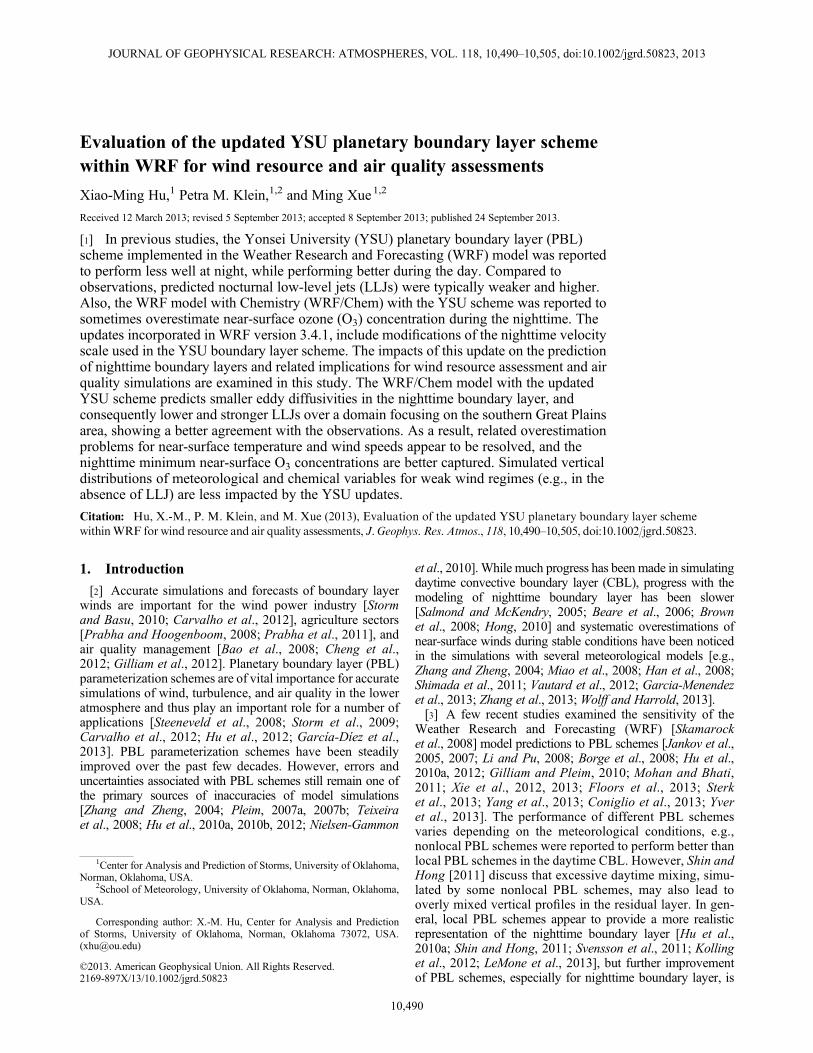
h is always smaller than 1and could be as small as 0.05 in the presence of strong verticalwind shear (e.g., in the presence of a low-level jet). Thus, thevalues of ϕm in the revised YSU scheme implemented inWRF version 3.4.1 are always larger than the correspondingvalues given by earlier versions. Example profiles of dimen-sionless Km using the two versions of ϕm are shown inFigure 1. The Km values using the updated ϕm (Figure 1b)are significantly smaller than those given by the old formu-lation (Figure 1a); the peak values of the Km profiles aregenerally reduced more than half, and are reduced evenmore for higher stability (i.e., larger values of h

L= ). Theheights of the profile peaks are also lower; effectively bring-ing the strongest mixing closer to the ground. The updatedprofiles (Figure 1b) appear to better capture the verticalmixing characteristics in the stable boundary layer [Brost

Figure 1. Vertical profiles of dimensionless momentumeddy diffusivity Km under different stabilities (different h/L)computed by the YSU scheme implemented in (a) the earlierversions of WRF (i.e., 3.4 and earlier) and (b) WRF 3.4.1.

10,491

HU ET AL.: IMPACT OF VERTICAL MIXING ON WIND AND O3

and Wyngaard, 1978]. Starting with version 3.4.1, an artificiallower limit for the velocity scale, ws ≥ u�

5 , found in the earlierversions of the YSU scheme has also been removed in additionto the change given in 3. The eddy diffusivity for scalars iscomputed from Km by dividing it by the Prandtl number Pr.It thus experiences a similar change as Km.[8] In this study, the impact of the modifications to the YSU

scheme on the prediction of boundary layer meteorology andair quality in the Great Plains for a low-level jets (LLJs) epi-sode in July 2003 is investigated in three-dimensional simula-tions using the WRF model including its Chemistry modelcomponent (WRF/Chem) [Grell et al., 2005]. The performanceof the YSU scheme is also assessed against simulations withWRF/Chem 3.4.1 using the Mellor-Yamada-Janjić [Janjic,1990] and Bougeault–Lacarrére [Bougeault and Lacarrere,1989] PBL schemes. These two PBL schemes were selectedfor the comparison because they both diagnose turbulent diffu-sion coefficient for scalars, which is required for WRF/Chemsimulations [Hu et al., 2012; Pleim, 2011] and because theywere widely used/evaluated for both meteorology and air

quality applications [e.g., Shin and Hong, 2011; Xie et al.,2012; LeMone et al., 2013; Žabkar et al., 2013]. MYJ andBouLac are both local TKE closure (one-and-a-half orderclosure) PBL schemes, but with different mixing length andmodel parameters. MYJ showed better performance duringstable conditions than some nonlocal scheme [Shin andHong, 2011; Draxl et al., 2012] while BouLac had a night-time overmixing problem when the mixing length is com-puted with the standard set of parameters of the scheme[Bravo et al., 2008].

2.2. Three-Dimensional Simulations

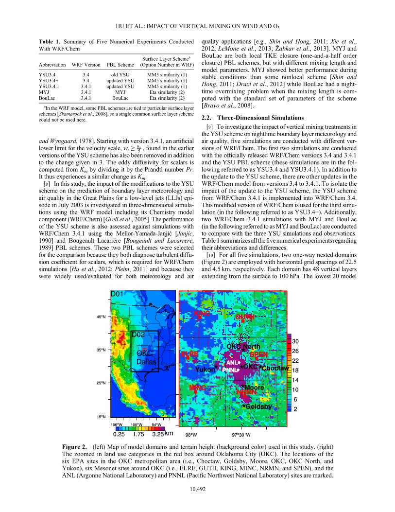
[9] To investigate the impact of vertical mixing treatments inthe YSU scheme on nighttime boundary layer meteorology andair quality, five simulations are conducted with different ver-sions of WRF/Chem. The first two simulations are conductedwith the officially released WRF/Chem versions 3.4 and 3.4.1and the YSU PBL scheme (these simulations are in the fol-lowing referred to as YSU3.4 and YSU3.4.1). In addition tothe update to the YSU scheme, there are other updates in theWRF/Chem model from versions 3.4 to 3.4.1. To isolate theimpact of the update to the YSU scheme, the YSU schemefrom WRF/Chem 3.4.1 is implemented into WRF/Chem 3.4.This modified version ofWRF/Chem is used for the third simu-lation (in the following referred to as YSU3.4+). Additionally,two WRF/Chem 3.4.1 simulations with MYJ and BouLac(in the following referred to asMYJ andBouLac) are conductedto compare with the three YSU simulations and observations.Table1summarizesall thefivenumerical experiments regardingtheir abbreviations and differences.[10] For all five simulations, two one-way nested domains

(Figure 2) are employed with horizontal grid spacings of 22.5and 4.5 km, respectively. Each domain has 48 vertical layersextending from the surface to 100 hPa. The lowest 20 model

Table 1. Summary of Five Numerical Experiments ConductedWith WRF/Chem

Abbreviation WRF Version PBL SchemeSurface Layer Schemea

(Option Number in WRF)

YSU3.4 3.4 old YSU MM5 similarity (1)YSU3.4+ 3.4 updated YSU MM5 similarity (1)YSU3.4.1 3.4.1 updated YSU MM5 similarity (1)MYJ 3.4.1 MYJ Eta similarity (2)BouLac 3.4.1 BouLac Eta similarity (2)

aIn the WRFmodel, some PBL schemes are tied to particular surface layerschemes [Skamarock et al., 2008], so a single common surface layer schemecould not be used here.

Figure 2. (left) Map of model domains and terrain height (background color) used in this study. (right)The zoomed in land use categories in the red box around Oklahoma City (OKC). The locations of thesix EPA sites in the OKC metropolitan area (i.e., Choctaw, Goldsby, Moore, OKC, OKC North, andYukon), six Mesonet sites around OKC (i.e., ELRE, GUTH, KING, MINC, NRMN, and SPEN), and theANL (Argonne National Laboratory) and PNNL (Pacific Northwest National Laboratory) sites are marked.

10,492


sigma levels are at 1.0, 0.997, 0.994, 0.991, 0.988, 0.985,0.975, 0.97, 0.96, 0.95, 0.94, 0.93, 0.92, 0.91, 0.895, 0.88,0.865, 0.85, 0.825, and 0.8 (the corresponding midlevelheights of each model layer are about 12, 37, 61, 86, 111,144, 186, 227, 290, 374, 459, 545, 631, 717, 826, 958, 1092,1226, and 1409m above ground). All model domains use theDudhia shortwave radiation algorithm [Dudhia, 1989], therapid radiative transfer model (RRTM) [Mlawer et al., 1997]for longwave radiation, the WRF Single-Moment 6-Class(WSM6) microphysics scheme [Hong et al., 2004], andthe Noah Land-Surface Scheme [Chen and Dudhia, 2001].For urban regions within domain 2 (shown in purple inFigure 2b), a single-layer urban canopy model (UCM) is usedfor land surface treatment. The 1° × 1° National Centers forEnvironmental Prediction (NCEP) Final (FNL) GlobalForecast System (GFS) analyses are used for the initial andboundary conditions of all meteorological variables (includ-ing soil properties). The inner grid gets its boundary condi-tions from the outer grid forecast.

[11] To determine gas phase chemical reactions, the RegionalAtmospheric ChemistryMechanism (RACM), [Stockwell et al.,1997] implemented within WRF/Chem is used. Hourlyanthropogenic emissions of chemical species come from the4 km×4km national emission inventory (NEI) for year 2005.Biogenic emissions are calculated using established algorithms[Guenther et al., 1994]. The focus of our modeling study isan episode (17–19 July 2003) during the Joint Urban 2003(JU2003) tracer experiment campaign in the Oklahoma City(OKC) metropolitan area [Allwine et al., 2004]. During thisepisode, the sky was clear, southerly/southwesterly wind dom-inated and moderate-strength LLJs occurred during the night-time [Lundquist and Mirocha, 2008; Hu et al., 2013b]. Thus,the episode is ideal for testing the impact of the update tothe YSU scheme for nighttime boundary layer, in particularfor examining if the updated YSU scheme has better skill insimulating LLJs. The simulations are initialized at 0000 UTC17 July and run until 0600 UTC 19 July 2003 without anydata assimilation. The initial and boundary conditions for the

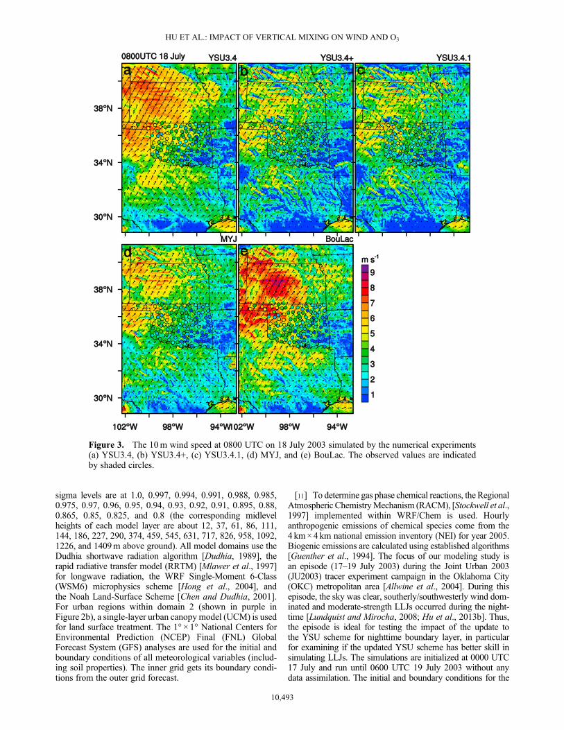
Figure 3. The 10m wind speed at 0800 UTC on 18 July 2003 simulated by the numerical experiments(a) YSU3.4, (b) YSU3.4+, (c) YSU3.4.1, (d) MYJ, and (e) BouLac. The observed values are indicatedby shaded circles.

10,493


chemical species are extracted from the output of the globalmodel MOZART4 with a resolution of 2.8° × 2.8° [Emmonset al., 2010]. Similar model configurations were used in previ-ous similar type of studies [e.g.,Hu et al., 2010c, 2012, 2013c;Klein et al., 2013].

2.3. Data Sets for Model Evaluation

[12] During the JU2003 tracer experiment, multiple meteo-rological observation systems were deployed across the OKCmetropolitan area. Boundary layer radar wind profilers andradiosonde are most relevant to the present study. The bound-ary layer wind profiler was operated almost continuouslyduring the entire month of July 2003 in OKC at the ArgonneNational Laboratory (ANL) site [De Wekker et al., 2004].The wind profiler collected data with a vertical resolution of55m and an average interval of 25min, providing coveragefrom 82m to ~ 2700m [De Wekker et al., 2004]. Radiosondeprofiles were taken at the Pacific Northwest NationalLaboratory (PNNL) site during four nighttime intensive observa-tional periods (IOPs). The episode chosen for this study is one ofthe IOPs, and temperature profiles from the radiosonde releasesduring the night are included for our model evaluation. ThePNNL and ANL sites were located approximately 2km southand 5km north of downtown OKC, respectively (Figure 2).[13] Meteorological data collected by the OklahomaMesonet

[McPherson et al., 2007] and O3 data collected at theEnvironmental Protection Agency (EPA) Air Quality System(AQS) sites (available at http://www.epa.gov/ttn/airs/airsaqs/detaildata/downloadaqsdata.htm) were additional data sources

used to evaluate the modeling results in this study. With anaverage spacing of approximately 30km between the Mesonetstations, there is at least one station in each Oklahoma county[Fiebrich and Crawford, 2001]. In contrast, the EPA AQS siteshave a much more inhomogeneous distribution. They are clus-tered near urban areas and are relatively sparse in rural areas.The meteorological variables considered in this study includedair temperature at 1.5m above ground level (AGL) and windspeed at 10m AGL.

3. Results of Numerical Experiments

3.1. Prediction of Boundary Layer Windand Temperature

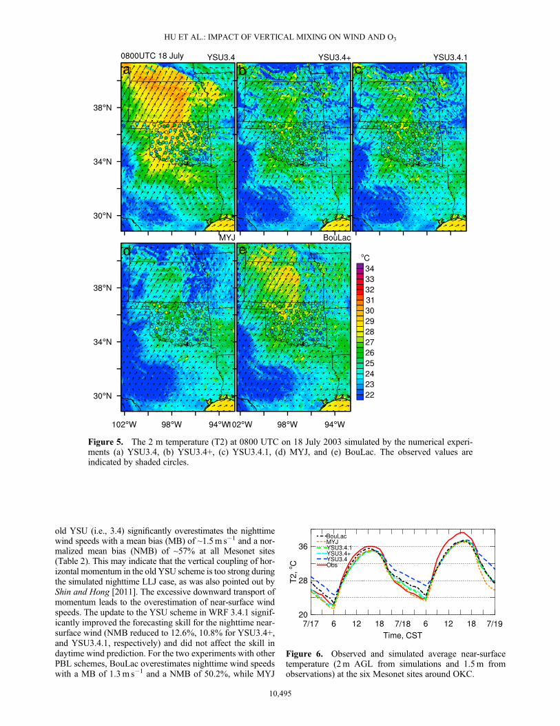
[14] Figure 3 shows the 10m wind speeds at 0800 UTC(0200 LST), 18 July 2003 from the five simulations, as com-pared to Mesonet observations shown by colored circles. It isclear that the simulated nighttime near-surface winds are im-proved considerably with the updated YSU PBL scheme. Inthe YSU3.4 simulation, near-surface winds are significantlyoverestimated, especially for central and western Oklahomawhere Mesonet data are available (Figure 3a); this problemis virtually eliminated in the YSU3.4.1 results (Figure 3c).The YSU3.4+ run, for which the updated YSU PBL schemewas implemented into WRF/Chem 3.4, shows similar resultsas the YSU3.4.1 simulation, indicating that the update to theYSU scheme plays a dominant role for the performance im-provement from WRF versions 3.4 to 3.4.1. A more detailedinvestigation of the differences between the YSU3.4+ andYSU3.4.1 results is beyond the scope of the study. For theexperiments with two other PBL schemes, MYJ simulatessimilar nighttime 10m wind as YSU3.4+ and YSU 3.4.1,while BouLac simulates the highest 10m wind speed, espe-cially for the western Oklahoma (Figure 3e).[15] Diurnal cycles of observed and simulated 10 m wind

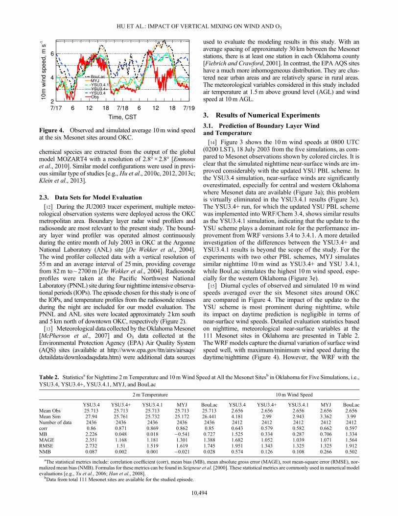
speeds averaged over the six Mesonet sites around OKCare compared in Figure 4. The impact of the update to theYSU scheme is most prominent during nighttime, whileits impact on daytime prediction is negligible in terms ofnear-surface wind speeds. Detailed evaluation statistics basedon nighttime, meteorological near-surface variables at the111 Mesonet sites in Oklahoma are presented in Table 2.TheWRFmodels capture the diurnal variation of surface windspeed well, with maximum/minimum wind speed during thedaytime/nighttime (Figure 4). However, the WRF with the

Figure 4. Observed and simulated average 10m wind speedat the six Mesonet sites around OKC.

Table 2. Statisticsa for Nighttime 2m Temperature and 10mWind Speed at All the Mesonet Sitesb in Oklahoma for Five Simulations, i.e.,YSU3.4, YSU3.4+, YSU3.4.1, MYJ, and BouLac

2m Temperature 10m Wind Speed

YSU3.4 YSU3.4+ YSU3.4.1 MYJ BouLac YSU3.4 YSU3.4+ YSU3.4.1 MYJ BouLacMean Obs 25.713 25.713 25.713 25.713 25.713 2.656 2.656 2.656 2.656 2.656Mean Sim 27.94 25.761 25.732 25.172 26.441 4.181 2.99 2.943 3.362 3.99Number of data 2436 2436 2436 2436 2436 2412 2412 2412 2412 2412corr 0.86 0.871 0.869 0.862 0.85 0.643 0.579 0.582 0.662 0.597MB 2.226 0.048 0.018 �0.541 0.727 1.525 0.334 0.287 0.706 1.334MAGE 2.351 1.168 1.181 1.301 1.388 1.682 1.052 1.039 1.071 1.564RMSE 2.732 1.51 1.519 1.619 1.745 1.951 1.343 1.325 1.325 1.912NMB 0.087 0.002 0.001 �0.021 0.028 0.574 0.126 0.108 0.266 0.502

aThe statistical metrics include: correlation coefficient (corr), mean bias (MB), mean absolute gross error (MAGE), root mean-square error (RMSE), nor-malized mean bias (NMB). Formulas for these metrics can be found in Seigneur et al. [2000]. These statistical metrics are commonly used in numerical modelevaluations [e.g., Yu et al., 2006; Han et al., 2008].

bData from total 111 Mesonet sites are available for the studied episode.

10,494


http://www.epa.gov/ttn/airs/airsaqs/detaildata/downloadaqsdata.htm

http://www.epa.gov/ttn/airs/airsaqs/detaildata/downloadaqsdata.htm

old YSU (i.e., 3.4) significantly overestimates the nighttimewind speeds with a mean bias (MB) of ~1.5m s�1 and a nor-malized mean bias (NMB) of ~57% at all Mesonet sites(Table 2). This may indicate that the vertical coupling of hor-izontal momentum in the old YSU scheme is too strong duringthe simulated nighttime LLJ case, as was also pointed out byShin and Hong [2011]. The excessive downward transport ofmomentum leads to the overestimation of near-surface windspeeds. The update to the YSU scheme in WRF 3.4.1 signif-icantly improved the forecasting skill for the nighttime near-surface wind (NMB reduced to 12.6%, 10.8% for YSU3.4+,and YSU3.4.1, respectively) and did not affect the skill indaytime wind prediction. For the two experiments with otherPBL schemes, BouLac overestimates nighttime wind speedswith a MB of 1.3m s�1 and a NMB of 50.2%, while MYJ

Figure 5. The 2 m temperature (T2) at 0800 UTC on 18 July 2003 simulated by the numerical experi-ments (a) YSU3.4, (b) YSU3.4+, (c) YSU3.4.1, (d) MYJ, and (e) BouLac. The observed values areindicated by shaded circles.

Figure 6. Observed and simulated average near-surfacetemperature (2m AGL from simulations and 1.5m fromobservations) at the six Mesonet sites around OKC.

10,495


performs similar as YSU3.4+/YSU3.4.1 in terms of RMSE(1.3m s�1) but worse in terms of MB (0.7m s�1) and NMB(26.6%) (Table 2).[16] Similar to near-surface winds (Figure 3), the WRF/

Chem simulations with the updated YSU PBL scheme (i.e.,YSU3.4+ and YSU3.4.1) show much better performancein predicting nighttime near-surface temperature than theYSU3.4 run (Figures 5, 6). The overestimation problem forthe nighttime 2 m temperature (T2) for YSU3.4 (with a MBof 2.2 °C at 111 Mesonet sites in Oklahoma) is nearly elimi-nated in the other two simulations (with aMB of 0.05, 0.02°Cfor YSU3.4+ and YSU3.4.1 respectively, Table 2). BouLacalso overestimates nighttime T2 by 0.7°C. Thus, BouLac hasa similar, but less severe, problem as the old YSU scheme tooverestimate nighttime near-surface wind speed and tempera-ture. MYJ gives a cold bias during nighttime with a MB of�0.5 °C presumably due to insufficient vertical mixing [Huet al., 2010a]. All the simulations underestimate the daytimepeak temperature (Figure 6), which might be due to othermodel errors (including the treatment of daytime boundarylayer) and/or inaccuracy in model initial conditions (e.g.,excessive soil moisture, [Hu et al., 2010a]).

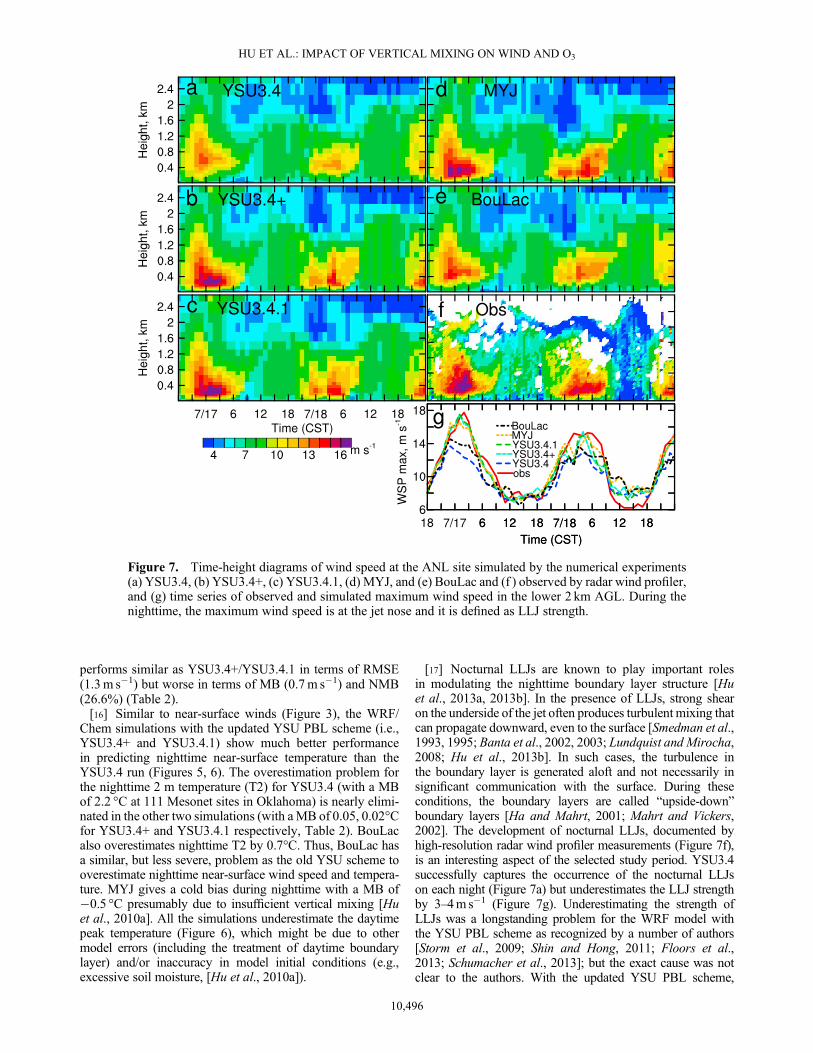
[17] Nocturnal LLJs are known to play important rolesin modulating the nighttime boundary layer structure [Huet al., 2013a, 2013b]. In the presence of LLJs, strong shearon the underside of the jet often produces turbulent mixing thatcan propagate downward, even to the surface [Smedman et al.,1993, 1995; Banta et al., 2002, 2003; Lundquist and Mirocha,2008; Hu et al., 2013b]. In such cases, the turbulence inthe boundary layer is generated aloft and not necessarily insignificant communication with the surface. During theseconditions, the boundary layers are called “upside-down”boundary layers [Ha and Mahrt, 2001; Mahrt and Vickers,2002]. The development of nocturnal LLJs, documented byhigh-resolution radar wind profiler measurements (Figure 7f),is an interesting aspect of the selected study period. YSU3.4successfully captures the occurrence of the nocturnal LLJson each night (Figure 7a) but underestimates the LLJ strengthby 3–4m s�1 (Figure 7g). Underestimating the strength ofLLJs was a longstanding problem for the WRF model withthe YSU PBL scheme as recognized by a number of authors[Storm et al., 2009; Shin and Hong, 2011; Floors et al.,2013; Schumacher et al., 2013]; but the exact cause was notclear to the authors. With the updated YSU PBL scheme,

Figure 7. Time-height diagrams of wind speed at the ANL site simulated by the numerical experiments(a) YSU3.4, (b) YSU3.4+, (c) YSU3.4.1, (d) MYJ, and (e) BouLac and (f ) observed by radar wind profiler,and (g) time series of observed and simulated maximum wind speed in the lower 2 km AGL. During thenighttime, the maximum wind speed is at the jet nose and it is defined as LLJ strength.

10,496


WRF/Chem simulates stronger LLJs (Figures 7b, 7c, 7g) thatpeak at lower levels, thus exhibiting a better agreement withthe observations (Figure 7f) in terms of the LLJs maximumwind speeds as well as their elevations. BouLac shows a sim-ilar behavior as YSU3.4, simulating weaker and higher LLJs(Figures 7e, 7g), while the MYJ results are again very similarto YSU3.4.1 (Figures 7d, 7g).[18] While wind profiles were measured continuously by

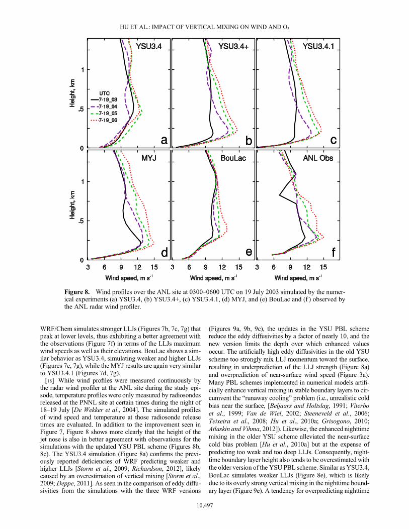
the radar wind profiler at the ANL site during the study epi-sode, temperature profiles were only measured by radiosondesreleased at the PNNL site at certain times during the night of18–19 July [De Wekker et al., 2004]. The simulated profilesof wind speed and temperature at those radiosonde releasetimes are evaluated. In addition to the improvement seen inFigure 7, Figure 8 shows more clearly that the height of thejet nose is also in better agreement with observations for thesimulations with the updated YSU PBL scheme (Figures 8b,8c). The YSU3.4 simulation (Figure 8a) confirms the previ-ously reported deficiencies of WRF predicting weaker andhigher LLJs [Storm et al., 2009; Richardson, 2012], likelycaused by an overestimation of vertical mixing [Storm et al.,2009; Deppe, 2011]. As seen in the comparison of eddy diffu-sivities from the simulations with the three WRF versions

(Figures 9a, 9b, 9c), the updates in the YSU PBL schemereduce the eddy diffusivities by a factor of nearly 10, and thenew version limits the depth over which enhanced valuesoccur. The artificially high eddy diffusivities in the old YSUscheme too strongly mix LLJ momentum toward the surface,resulting in underprediction of the LLJ strength (Figure 8a)and overprediction of near-surface wind speed (Figure 3a).Many PBL schemes implemented in numerical models artifi-cially enhance vertical mixing in stable boundary layers to cir-cumvent the “runaway cooling” problem (i.e., unrealistic coldbias near the surface, [Beljaars and Holtslag, 1991; Viterboet al., 1999; Van de Wiel, 2002; Steeneveld et al., 2006;Teixeira et al., 2008; Hu et al., 2010a; Grisogono, 2010;Atlaskin and Vihma, 2012]). Likewise, the enhanced nighttimemixing in the older YSU scheme alleviated the near-surfacecold bias problem [Hu et al., 2010a] but at the expense ofpredicting too weak and too deep LLJs. Consequently, night-time boundary layer height also tends to be overestimated withthe older version of the YSU PBL scheme. Similar as YSU3.4,BouLac simulates weaker LLJs (Figure 8e), which is likelydue to its overly strong vertical mixing in the nighttime bound-ary layer (Figure 9e). A tendency for overpredicting nighttime

Figure 8. Wind profiles over the ANL site at 0300–0600 UTC on 19 July 2003 simulated by the numer-ical experiments (a) YSU3.4, (b) YSU3.4+, (c) YSU3.4.1, (d) MYJ, and (e) BouLac and (f ) observed bythe ANL radar wind profiler.

10,497


mixing with the BouLac scheme was also reported in Bravoet al. [2008].[19] The artificially strong vertical mixing (illustrated by

eddy diffusivities shown in Figure 9a) also affects the temper-ature structure resulting in an underprediction of nighttimenear-surface inversion strength (Figure 10a). With the updatedYSU PBL scheme, temperature profiles in the boundary layercompare better with the radiosonde observations, showing a

more stable regime near the surface (Figures 10b, 10c). Dueto its strong vertical mixing (Figure 9e), BouLac also simu-lates weaker stratification below 0.2 km AGL (Figure 10e)than the other PBL schemes. The vertical structure of theboundary layer plays an important role and should be carefullyconsidered during model evaluation and improvement studies,while previous operational studies typically exclusively fo-cused on near-surface variables [Draxl et al., 2012; Sterk

Figure 9. Vertical profiles of eddy diffusivity over the ANL site at 0300–0600 UTC on 19 July 2003 sim-ulated by the numerical experiments (a) YSU3.4, (b) YSU3.4+, (c) YSU3.4.1, (d) MYJ, and (e) BouLac.

Figure 10. Profiles of potential temperature over the PNNL site at 0300–0600 UTC on 19 July 2003 sim-ulated by the numerical experiments (a) YSU3.4, (b) YSU3.4+, (c) YSU3.4.1, (d) MYJ, and (e) BouLac,and (f ) observed by radiosondes.

10,498


et al., 2013; Zhang et al., 2013]. An elevated inversion layerwas observed at ~1.6 km AGL (Figure 10f). All five simula-tions capture this elevated inversion, but differences can benoted in the predicted strength and height of the inversionlayer. During nighttime, vertical mixing at this altitude issuppressed and the elevated inversion is the remnant of thetop boundary of the daytime CBL. Thus, strength and heightof the simulated elevated inversion are affected by the treat-ment of the daytime CBL. The MYJ and BouLac schemessimulate a lower daytime PBL (figure not shown) due to theirweaker daytime vertical mixing and weaker entrainment at theCBL top [Hu et al., 2010; LeMone et al., 2013]. Consequently,MYJ and BouLac predict the inversion layer at lower eleva-tions (just above 1 km) (Figures 10d, 10e). All the schemestend to underestimate the strength of the elevated inversion,which might be due to model uncertainties associated withvertical mixing in the residual layer and the free troposphere[Hu et al., 2012] and/or insufficient vertical model resolution.[20] Vertical mixing in the boundary layer also impacts the

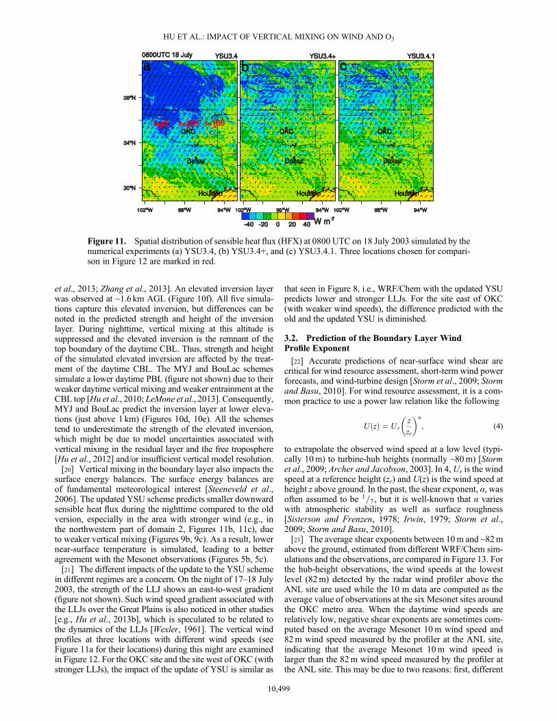
surface energy balances. The surface energy balances areof fundamental meteorological interest [Steeneveld et al.,2006]. The updated YSU scheme predicts smaller downwardsensible heat flux during the nighttime compared to the oldversion, especially in the area with stronger wind (e.g., inthe northwestern part of domain 2, Figures 11b, 11c), dueto weaker vertical mixing (Figures 9b, 9c). As a result, lowernear-surface temperature is simulated, leading to a betteragreement with the Mesonet observations (Figures 5b, 5c).[21] The different impacts of the update to the YSU scheme

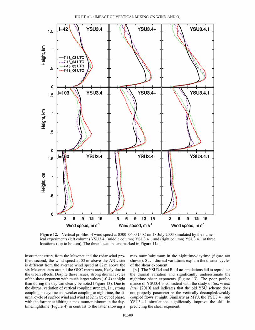
in different regimes are a concern. On the night of 17–18 July2003, the strength of the LLJ shows an east-to-west gradient(figure not shown). Such wind speed gradient associated withthe LLJs over the Great Plains is also noticed in other studies[e.g., Hu et al., 2013b], which is speculated to be related tothe dynamics of the LLJs [Wexler, 1961]. The vertical windprofiles at three locations with different wind speeds (seeFigure 11a for their locations) during this night are examinedin Figure 12. For the OKC site and the site west of OKC (withstronger LLJs), the impact of the update of YSU is similar as

that seen in Figure 8, i.e., WRF/Chem with the updated YSUpredicts lower and stronger LLJs. For the site east of OKC(with weaker wind speeds), the difference predicted with theold and the updated YSU is diminished.

3.2. Prediction of the Boundary Layer WindProfile Exponent

[22] Accurate predictions of near-surface wind shear arecritical for wind resource assessment, short-term wind powerforecasts, and wind-turbine design [Storm et al., 2009; Stormand Basu, 2010]. For wind resource assessment, it is a com-mon practice to use a power law relation like the following

U zð Þ ¼ Urz

zr

� �α

; (4)

to extrapolate the observed wind speed at a low level (typi-cally 10m) to turbine-hub heights (normally ~80m) [Stormet al., 2009; Archer and Jacobson, 2003]. In 4,Ur is the windspeed at a reference height (zr) and U(z) is the wind speed atheight z above ground. In the past, the shear exponent, α, wasoften assumed to be 1

7= , but it is well-known that α varieswith atmospheric stability as well as surface roughness[Sisterson and Frenzen, 1978; Irwin, 1979; Storm et al.,2009; Storm and Basu, 2010].[23] The average shear exponents between 10m and ~82m

above the ground, estimated from different WRF/Chem sim-ulations and the observations, are compared in Figure 13. Forthe hub-height observations, the wind speeds at the lowestlevel (82m) detected by the radar wind profiler above theANL site are used while the 10 m data are computed as theaverage value of observations at the six Mesonet sites aroundthe OKC metro area. When the daytime wind speeds arerelatively low, negative shear exponents are sometimes com-puted based on the average Mesonet 10m wind speed and82m wind speed measured by the profiler at the ANL site,indicating that the average Mesonet 10m wind speed islarger than the 82m wind speed measured by the profiler atthe ANL site. This may be due to two reasons: first, different

Figure 11. Spatial distribution of sensible heat flux (HFX) at 0800 UTC on 18 July 2003 simulated by thenumerical experiments (a) YSU3.4, (b) YSU3.4+, and (c) YSU3.4.1. Three locations chosen for compari-son in Figure 12 are marked in red.

10,499


instrument errors from the Mesonet and the radar wind pro-filer; second, the wind speed at 82m above the ANL siteis different from the average wind speed at 82m above thesix Mesonet sites around the OKC metro area, likely due tothe urban effects. Despite these issues, strong diurnal cyclesof the shear exponent with much larger values (~0.4) at nightthan during the day can clearly be noted (Figure 13). Due tothe diurnal variation of vertical coupling strength, i.e., strongcoupling in daytime and weaker coupling at nighttime, the di-urnal cycle of surface wind and wind at 82m are out of phase,with the former exhibiting a maximum/minimum in the day-time/nighttime (Figure 4) in contrast to the latter showing a

maximum/minimum in the nighttime/daytime (figure notshown). Such diurnal variations explain the diurnal cyclesof the shear exponent.[24] The YSU3.4 and BouLac simulations fail to reproduce

the diurnal variation and significantly underestimate thenighttime shear exponents (Figure 13). The poor perfor-mance of YSU3.4 is consistent with the study of Storm andBasu [2010] and indicates that the old YSU scheme doesnot properly parameterize the vertically decoupled/weaklycoupled flows at night. Similarly as MYJ, the YSU3.4+ andYSU3.4.1 simulations significantly improve the skill inpredicting the shear exponent.

Figure 12. Vertical profiles of wind speed at 0300–0600 UTC on 18 July 2003 simulated by the numer-ical experiments (left column) YSU3.4, (middle column) YSU3.4+, and (right column) YSU3.4.1 at threelocations (top to bottom). The three locations are marked in Figure 11a.

10,500


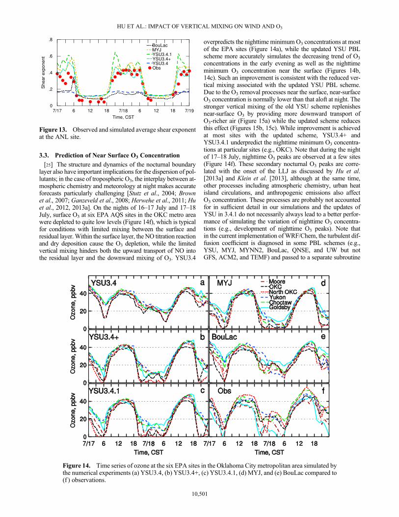
3.3. Prediction of Near Surface O3 Concentration

[25] The structure and dynamics of the nocturnal boundarylayer also have important implications for the dispersion of pol-lutants; in the case of tropospheric O3, the interplay between at-mospheric chemistry and meteorology at night makes accurateforecasts particularly challenging [Stutz et al., 2004; Brownet al., 2007; Ganzeveld et al., 2008; Herwehe et al., 2011; Huet al., 2012, 2013a]. On the nights of 16–17 July and 17–18July, surface O3 at six EPA AQS sites in the OKC metro areawere depleted to quite low levels (Figure 14f), which is typicalfor conditions with limited mixing between the surface andresidual layer.Within the surface layer, the NO titration reactionand dry deposition cause the O3 depletion, while the limitedvertical mixing hinders both the upward transport of NO intothe residual layer and the downward mixing of O3. YSU3.4

overpredicts the nighttime minimumO3 concentrations at mostof the EPA sites (Figure 14a), while the updated YSU PBLscheme more accurately simulates the decreasing trend of O3

concentrations in the early evening as well as the nighttimeminimum O3 concentration near the surface (Figures 14b,14c). Such an improvement is consistent with the reduced ver-tical mixing associated with the updated YSU PBL scheme.Due to the O3 removal processes near the surface, near-surfaceO3 concentration is normally lower than that aloft at night. Thestronger vertical mixing of the old YSU scheme replenishesnear-surface O3 by providing more downward transport ofO3-richer air (Figure 15a) while the updated scheme reducesthis effect (Figures 15b, 15c). While improvement is achievedat most sites with the updated scheme, YSU3.4+ andYSU3.4.1 underpredict the nighttime minimum O3 concentra-tions at particular sites (e.g., OKC). Note that during the nightof 17–18 July, nighttime O3 peaks are observed at a few sites(Figure 14f). These secondary nocturnal O3 peaks are corre-lated with the onset of the LLJ as discussed by Hu et al.[2013a] and Klein et al. [2013], although at the same time,other processes including atmospheric chemistry, urban heatisland circulations, and anthropogenic emissions also affectO3 concentration. These processes are probably not accountedfor in sufficient detail in our simulations and the updates ofYSU in 3.4.1 do not necessarily always lead to a better perfor-mance of simulating the variation of nighttime O3 concentra-tions (e.g., development of nighttime O3 peaks). Note thatin the current implementation ofWRF/Chem, the turbulent dif-fusion coefficient is diagnosed in some PBL schemes (e.g.,YSU, MYJ, MYNN2, BouLac, QNSE, and UW but notGFS, ACM2, and TEMF) and passed to a separate subroutine

Figure 13. Observed and simulated average shear exponentat the ANL site.

Figure 14. Time series of ozone at the six EPA sites in the Oklahoma City metropolitan area simulated bythe numerical experiments (a) YSU3.4, (b) YSU3.4+, (c) YSU3.4.1, (d) MYJ, and (e) BouLac compared to(f ) observations.

10,501


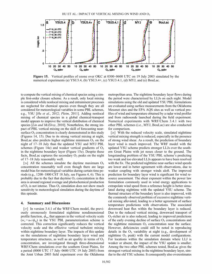
to compute the vertical mixing of chemical species using a sim-ple first-order closure scheme. As a result, only local mixingis considered while nonlocal mixing and entrainment processesare neglected for chemical species even though they are allconsidered for meteorological variables in some PBL schemes,e.g., YSU [Hu et al., 2012; Pleim, 2011]. Adding nonlocalmixing of chemical species in a global chemical-transportmodel appears to improve the vertical distribution of chemicalspecies [Lin and McElroy, 2010]. Nonetheless, the strong im-pact of PBL vertical mixing on the skill of forecasting near-surface O3 concentration is clearly demonstrated in this study(Figures 14, 15). Due to its strong vertical mixing at night,BouLac also predicts higher nighttime minimum O3 on thenight of 17–18 July than the updated YSU and MYJ PBLschemes (Figure 14e) and weaker vertical gradients of O3

in the nighttime boundary layer (Figure 15e). Despite thesefacts, BouLac captures the secondary O3 peaks on the nightof 17–18 July reasonably well.[26] All the schemes simulate the daytime maximum O3

concentration reasonably well even though there are largemodel bias for meteorological variables during certain time pe-riods (e.g., 1200–1800 CST 18 July, see Figures 4, 6). This isprobably due to the fact that daytime O3 concentration in thisarea is around regional average and photochemical productionof O3 is not intense. Thus O3 simulation does not show muchsensitivity to meteorological simulation during the daytime ofthis episode.

4. Summary and Discussions

[27] In version 3.4.1 of the WRF/Chem model, the previ-ously erroneously formulated nighttime nondimensionalprofile function,ϕm, that appears in the vertical velocity scale(ws = u*/ϕm) in the YSU PBL parameterization scheme iscorrected. This correction significantly reduces the verticalvelocity scale and the effective vertical turbulent mixingwithin nighttime boundary layer. The impacts of this updateon the simulations of nighttime boundary layer wind andtemperature structures, as well as air quality in terms of O3

concentration, are investigated through three-dimensionalWRF/Chem simulations over the southern Great Plains, fora period (0000 UTC 17 July–0600 UTC 19 July 2003) fromthe Joint Urban 2003 field experiment over the Oklahoma

metropolitan area. The nighttime boundary layer flows duringthe period were characterized by LLJs on each night. Modelsimulations using the old and updated YSU PBL formulationsare evaluated using surface measurements from the OklahomaMesonet sites and the EPA AQS sites as well as vertical pro-files of wind and temperature obtained by a radar wind profilerand from radiosonde launched during the field experiment.Numerical experiments with WRF/Chem 3.4.1 with twoother PBL schemes (i.e., MYJ, BouLac) are also conductedfor comparison.[28] With the reduced velocity scale, simulated nighttime

vertical mixing strength is reduced, especially in the presenceof strong wind shear. As a result, the prediction of boundarylayer wind is much improved. The WRF model with theupdated YSU scheme predicts stronger LLJs over the south-ern Great Plains with jet noses closer to the ground. Thelongstanding problem of the YSU PBL scheme’s predictingtoo weak and too elevated LLJs appears to have been resolvedwith the fix. The predicted nighttime near-surface wind speedsare lower and in better agreement with observations, due toweaker coupling with stronger winds aloft. The improvedprediction for boundary layer wind is significant for wind re-source assessment. The shear exponent within the power lawformulation commonly used in wind energy applications toextrapolate wind speed from a reference height is better simu-lated during nighttime with the updated YSU scheme. Thethermal structure of the boundary layer is also improved, withthe commonly observed problem of excessive nighttime verti-cal mixing alleviated, leading to a better agreement of surfacetemperature predictions with observations. The associateddownward heat flux within the boundary layer is reduced.Due to the reduced vertical mixing, downward transport ofO3-richer air is also reduced, leading to improved predictionsof the early evening decline of surface O3 concentrations andthe nighttime minimum O3 concentration near the surface.However, deficiencies could still be noted in reproducingdetails in the O3 variability at night (e.g., development ofnighttime O3 peak) with the current model configurations.For locations within the simulation domain where LLJ isweaker or absent, the impact of the YSU update is smaller.Among the two other PBL schemes tested, BouLac gives thestrongest vertical mixing in the nighttime boundary layer, sim-ilar to the old YSU scheme. It consequently also overestimates

Figure 15. Vertical profiles of ozone over OKC at 0300–0600 UTC on 19 July 2003 simulated by thenumerical experiments (a) YSU3.4, (b) YSU3.4+, (c) YSU3.4.1, (d) MYJ, and (e) BouLac.

10,502


near-surface wind and temperature and underestimates thewind shear exponent at night. However, BouLac captures thenighttime secondary O3 peaks reasonably well.[29] In most previous model evaluation studies [e.g., Berg

and Zhong, 2005; Srinivas et al., 2007; Sanjay, 2008; Huet al., 2010a], PBL schemes are mostly evaluated for the “tra-ditional” boundary layer, in which turbulence is generated atthe surface and transported upward. There are very few com-prehensive evaluations of PBL schemes for the “upside-down” boundary layer, in which turbulence is produced aloftand transported downward [Todd et al., 2008; Carter et al.,2011]. Further evaluation of model simulations with differentPBL schemes, along with the collection of more suitableobservations (e.g., turbulence profiles in the presence ofLLJs), for the “upside-down” boundary layers is warrantedfor providing guidance to future model improvement [Deppe,2011; Deppe et al., 2013; Banta et al., 2013].

[30] Acknowledgments. This work was supported by funding from theOffice of the Vice President for Research at the University of Oklahoma. Thesecond author was also supported through the NSF Career award ILREUM(NSF ATM 0547882). The third author was also supported by NSF grantsOCI-0905040, AGS-0802888, AGS-0750790, AGS-0941491, AGS-1046171,and AGS-1046081. Computations were performed at the Texas AdvancedComputing Center (TACC). Discussion with Songyou Hong helped to confirmthe code updates from WRF versions 3.4 to 3.4.1. Proofreading by David C.Doughty is greatly appreciated. Four anonymous reviewers provided helpfulcomments that improved the manuscript.

ReferencesArcher, C. L., and M. Z. Jacobson (2003), Spatial and temporal distributionsof US winds and wind power at 80m derived from measurements,J. Geophys. Res., 108(D9), 4289, doi:10.1029/2002JD002076.

Arnold, J. R., and R. L. Dennis (2001), First results from operational testing ofthe U.S. EPA Models-3/Community Multiscale Model for Air Quality(CMAQ), in Air Pollution Modeling and Its Application XIV, edited by S.-E.Gryning and F. A. Schiermeier, pp. 651–658, Kluwer Acad., Norwell, Mass.

Atlaskin, E., and T. Vihma (2012), Evaluation of NWP results for wintertimenocturnal boundary layer temperatures over Europe and Finland,Q. J. RoyMeteor. Soc., 138(667), 1440–1451, doi:10.1002/Qj.1885.

Banta, R. M., R. K. Newsom, J. K. Lundquist, Y. L. Pichugina, R. L. Coulter,and L. Mahrt (2002), Nocturnal low-level jet characteristics over Kansasduring CASES-99, Bound-Lay Meteorol., 105(2), 221–252, doi:10.1023/A:1019992330866.

Banta, R. M., Y. L. Pichugina, and R. K. Newsom (2003), Relationshipbetween low-level jet properties and turbulence kinetic energy in thenocturnal stable boundary layer, J. Atmos. Sci., 60(20), 2549–2555,doi:10.1175/1520-0469(2003)060<2549:Rbljpa>2.0.Co;2.

Banta, R. M., Y. L. Pichugina, N. D. Kelley, R. M. Hardesty, andW. A. Brewer (2013), Wind Energy Meteorology: Insight into wind prop-erties in the turbine-rotor layer of the atmosphere from high-resolutiondoppler lidar, Bull. Am. Meteorol. Soc., 94(6), 883–902, doi:10.1175/Bams-D-11-00057.1.

Bao, J.W., S. A.Michelson, P. O. G. Persson, I. V. Djalalova, and J.M.Wilczak(2008), Observed and WRF-simulated low-level winds in a high-ozone epi-sode during the Central California Ozone Study, J. Appl. Meteorol. Climatol.,47(9), 2372–2394, doi:10.1175/2008jamc1822.1.

Beare, R. J., et al. (2006), An intercomparison of large-eddy simulations of thestable boundary layer, Bound-Lay Meteorol., 118(2), 247–272, doi:10.1007/s10546-004-2820-6.

Beljaars, A. C. M., and A. A. M. Holtslag (1991), Flux Parameterizationover Land Surfaces for Atmospheric Models, J. Appl. Meteorol., 30(3),327–341, doi:10.1175/1520-0450(1991)030<0327:Fpolsf>2.0.Co;2.

Berg, L. K., and S. Y. Zhong (2005), Sensitivity of MM5-simulated boundarylayer characteristics to turbulence parameterizations, J. Appl. Meteorol.,44(9), 1467–1483, doi:10.1175/Jam2292.1.

Borge, R., V. Alexandrov, J. J. del Vas, J. Lumbreras, and E. Rodriguez(2008), A comprehensive sensitivity analysis of the WRF model for airquality applications over the Iberian Peninsula, Atmos. Environ., 42(37),8560–8574, doi:10.1016/j.atmosenv.2008.08.032.

Bougeault, P., and P. Lacarrere (1989), Parameterization of orography-inducedturbulence in a mesobeta-scale model, Mon. Weather Rev., 117(8),1872–1890, doi:10.1175/1520-0493(1989)117<1872:Pooiti>2.0.Co;2.

Bravo,M., T.Mira,M. R. Soler, and J. Cuxart (2008), Intercomparison and eval-uation ofMM5 andMeso-NHmesoscalemodels in the stable boundary layer,Bound-Lay Meteorol., 128(1), 77–101, doi:10.1007/s10546-008-9269-y.

Brost, R. A., and J. C. Wyngaard (1978), A model study of the stablystratified planetary boundary layer, J. Atmos. Sci., 35(8), 1427–1440,doi:10.1175/1520-0469(1978)035<1427:amsots>2.0.co;2.

Brown, S. S., W. P. Dubé, H. D. Osthoff, D. E. Wolfe, W. M. Angevine, andA. R. Ravishankara (2007), High resolution vertical distributions of NO3and N2O5 through the nocturnal boundary layer, Atmos. Chem. Phys.,7(1), 139–149, doi:10.5194/acp-7-139-2007.

Brown, A. R., R. J. Beare, J. M. Edwards, A. P. Lock, S. J. Keogh,S. F. Milton, and D. N. Walters (2008), Upgrades to the boundary layerscheme in the Met Office numerical weather prediction model, Bound-Lay Meteorol., 128(1), 117–132, doi:10.1007/s10546-008-9275-0.

Carter, K. C., A. J. Deppe, and W. A. Gallus (2011), Simulations of noctur-nal LLJs with a WRF PBL scheme ensemble and comparison to observa-tions from the ARM project. 20th Conf. on Numerical Weather Prediction,Seattle, WA, Amer. Meteor. Soc. P474.

Carvalho, D., A. Rocha, M. Gomez-Gesteira, and C. Santos (2012), Asensitivity study of the WRF model in wind simulation for an area ofhigh wind energy, Environ. Modell. Software, 33, 23–34, doi:10.1016/j.envsoft.2012.01.019.

Chen, F., and J. Dudhia (2001), Coupling an advanced land surface-hydrologymodel with the Penn State-NCAR MM5 modeling system. Part I: Modelimplementation and sensitivity, Mon. Weather Rev., 129(4), 569–585,doi:10.1175/1520-0493(2001)129<0569:Caalsh>2.0.Co;2.

Chen, J. J., H. T.Mao, R.W. Talbot, and R. J. Griffin (2006), Application of theCACM and MPMPO modules using the CMAQ model for the easternUnited States, J. Geophys. Res., 111, D23S25, doi:10.1029/2006JD007603.

Chen, J., J. Vaughan, J. Avise, S. O’Neill, and B. Lamb (2008),Enhancement and evaluation of the AIRPACT ozone and PM2.5 forecastsystem for the Pacific Northwest, J. Geophys. Res., 113, D14305,doi:10.1029/2007JD009554.

Cheng, F. Y., S. C. Chin, and T. H. Liu (2012), The role of boundary layerschemes in meteorological and air quality simulations of the Taiwan area,Atmos. Environ., 54, 714–727, doi:10.1016/j.atmosenv.2012.01.029.

Coniglio, M. C., J. Correia, P. T. Marsh, and F. Kong (2013), Verification ofconvection-allowing WRF model forecasts of the planetary boundarylayer using sounding observations, Weather Forecast, 28(3), 842–862,doi:10.1175/Waf-D-12-00103.1.

De Wekker, S. F. J., L. K. Berg, J. Allwine, J. C. Doran, and W. J. Shaw(2004), Boundary-layer structure upwind and downwind of OklahomaCity during the Joint Urban 2003 field study. Preprints. Fifth Conf.on Urban Environment, Vancouver, BC, Canada, Amer. Meteor. Soc.,CD-ROM, 3.20.

Deppe, A. J. (2011), Improvements in numerical prediction of low levelwinds. Graduate Theses and Dissertations. Paper 10100. http://lib.dr.iastate.edu/etd/10100.

Deppe, A. J., W. A. Gallus, and E. S. Takle (2013), A WRF ensemble forimproved wind speed forecasts at turbine height, Weather Forecast,28(1), 212–228, doi:10.1175/WAF-D-11-00112.1.

Draxl, C., A. N. Hahmann, A. Peña, and G. Giebel (2012), Evaluating windsand vertical wind shear from Weather Research and Forecasting modelforecasts using seven planetary boundary layer schemes, Wind Energy,doi:10.1002/we.1555.

Dudhia, J. (1989), Numerical study of convection observed during thewinter monsoon experiment using a mesoscale two-dimensionalmodel, J. Atmos. Sci., 46(20), 3077–3107, doi:10.1175/1520-0469(1989)046<3077:Nsocod>2.0.Co;2.

Eder, B., D. W. Kang, R. Mathur, S. C. Yu, and K. Schere (2006), An oper-ational evaluation of the Eta-CMAQ air quality forecast model, Atmos.Environ., 40(26), 4894–4905, doi:10.1016/j.atmonsenv.2005.12.062.

Emmons, L. K., et al. (2010), Description and evaluation of the Model forOzone and Related Chemical Tracers, version 4 (MOZART-4), Geosci.Model Dev., 3(1), 43–67, doi:10.5194/gmd-3-43-2010.

Engardt, M. (2008), Modelling of near-surface ozone over South Asia,J. Atmos. Chem., 59(1), 61–80, doi:10.1007/s10874-008-9096-z.

Fernando, H. J. S., and J. C. Weil (2010), Whither the stable boundary layer?A shift in the research agenda, Bull. Am. Meteorol. Soc., 91(11), 1475–1484,doi:10.1175/2010bams2770.1.

Fiebrich, C. A., and K. C. Crawford (2001), The impact of unique meteorolog-ical phenomena detected by the Oklahoma Mesonet and ARS Micronet onautomated quality control, Bull. Am. Meteorol. Soc., 82(10), 2173–2187,doi:10.1175/1520-0477(2001)082<2173:Tioump>2.3.Co;2.

Floors, R., C. L. Vincent, S. E. Gryning, A. Peña, and E. Batchvarova(2013), The wind profile in the coastal boundary layer: Wind lidar mea-surements and numerical modelling, Bound-Lay Meteorol., 147(3),469–491, doi:10.1007/s10546-012-9791-9.

Ganzeveld, L., et al. (2008), Surface and boundary layer exchanges of vola-tile organic compounds, nitrogen oxides and ozone during the GABRIEL

10,503


http://lib.dr.iastate.edu/etd/10100

http://lib.dr.iastate.edu/etd/10100

campaign, Atmos. Chem. Phys., 8(20), 6223–6243, doi:10.5194/acp-8-6223-2008.

García-Díez, M., J. Fernández, L. Fita, and C. Yagüe (2013), Seasonal de-pendence of WRF model biases and sensitivity to PBL schemes overEurope, Quart. J. Roy. Meteor. Soc., 139(671), 501–514, doi:10.1002/qj.1976.

Garcia-Menendez, F., Y. Hu, andM. T. Odman (2013), Simulating smoke trans-port from wildland fires with a regional-scale air quality model: Sensitivity touncertain wind fields, J Geophys Res. Atmos, 118, 6493–6504, doi:10.1002/jgrd.50524.

Gilliam, R. C., and J. E. Pleim (2010), Performance assessment of new landsurface and planetary boundary layer physics in the WRF-ARW, J. Appl.Meteorol. Climatol., 49(4), 760–774, doi:10.1175/2009jamc2126.1.

Gilliam, R. C., J. M. Godowitch, and S. T. Rao (2012), Improving the horizon-tal transport in the lower troposphere with four dimensional data assimila-tion, Atmos. Environ., 53, 186–201, doi:10.1016/j.atmosenv.2011.10.064.

Grell, G. A., S. E. Peckham, R. Schmitz, S. A. McKeen, G. Frost,W. C. Skamarock, and B. Eder (2005), Fully coupled “online” chemistrywithin the WRF model, Atmos. Environ., 39(37), 6957–6975, doi:10.1016/j.atmosenv.2005.04.027.

Grisogono, B. (2010), Generalizing ’z-less’ mixing length for stable bound-ary layers, Quart. J. Roy. Meteor. Soc., 136(646), 213–221, doi:10.1002/Qj.529.

Grisogono, B., and D. Belusic (2008), Improving mixing length-scale forstable boundary layers, Quart. J. Roy. Meteor. Soc., 134(637), 2185–2192,doi:10.1002/Qj.347.

Guenther, A., P. Zimmerman, and M. Wildermuth (1994), Natural volatileorganic-compound emission rate estimates for United-States woodlandlandscapes, Atmos. Environ., 28(6), 1197–1210, doi:10.1016/1352-2310(94)90297-6.

Ha, K. J., and L. Mahrt (2001), Simple inclusion of z-less turbulence within andabove the modeled nocturnal boundary layer, Mon. Weather Rev., 129(8),2136–2143, doi:10.1175/1520-0493(2001)129<2136:Siozlt>2.0.Co;2.

Han, Z.W., H. Ueda, and J. L. An (2008), Evaluation and intercomparison ofmeteorological predictions by fiveMM5-PBL parameterizations in combi-nation with three land-surface models, Atmos. Environ., 42(2), 233–249,doi:10.1016/j.atmosenv.2007.09.053.

Hanna, S. R., and R. X. Yang (2001), Evaluations of mesoscale models’ sim-ulations of near-surface winds, temperature gradients, and mixing depths,J. Appl. Meteorol., 40(6), 1095–1104, doi:10.1175/1520-0450(2001)040<1095:Eommso>2.0.Co;2.

Herwehe, J. A., T. L. Otte, R. Mathur, and S. T. Rao (2011), Diagnosticanalysis of ozone concentrations simulated by two regional-scale airquality models, Atmos. Environ., 45(33), 5957–5969, doi:10.1016/j.atmosenv.2011.08.011.

Hong, S. Y. (2010), A new stable boundary layer mixing scheme and itsimpact on the simulated East Asian summer monsoon, Quart. J. Roy.Meteor. Soc., 136(651), 1481–1496, doi:10.1002/Qj.665.

Hong, S. Y., J. Dudhia, and S. H. Chen (2004), A revised approach to icemicrophysical processes for the bulk parameterization of clouds andprecipitation, Mon. Weather Rev., 132(1), 103–120, doi:10.1175/1520-0493(2004)132<0103:Aratim>2.0.Co;2.

Hong, S. Y., Y. Noh, and J. Dudhia (2006), A new vertical diffusion packagewith an explicit treatment of entrainment processes, Mon. Weather Rev.,134(9), 2318–2341, doi:10.1175/Mwr3199.1.

Hu, X.-M. (2008), Incorporation of the Model of Aerosol Dynamics, Reaction,Ionization, and Dissolution (MADRID) into the Weather Research andForecasting Model with Chemistry (WRF/Chem): Model development andretrospective applications, Ph.D. dissertation, N. C. State Univ., Raleigh,July. http://repository.lib.ncsu.edu/ir/handle/1840.16/5241.

Hu, X.-M., J. W. Nielsen-Gammon, and F. Q. Zhang (2010a), Evaluation ofthree planetary boundary layer schemes in the WRF model, J. Appl.Meteorol. Climatol., 49(9), 1831–1844, doi:10.1175/2010jamc2432.1.

Hu, X.-M., F. Q. Zhang, and J. W. Nielsen-Gammon (2010b), Ensemble-based simultaneous state and parameter estimation for treatment of meso-scale model error: A real-data study, Geophys. Res. Lett., 37, L08802,doi:10.1029/2010GL043017.

Hu, X.-M., J. D. Fuentes, and F. Q. Zhang (2010c), Downward transport andmodification of tropospheric ozone through moist convection, J. Atmos.Chem., 65(1), 13–35, doi:10.1007/s10874-010-9179-5.

Hu, X.-M., D. C. Doughty, K. J. Sanchez, E. Joseph, and J. D. Fuentes(2012), Ozone variability in the atmospheric boundary layer in Marylandand its implications for vertical transport model, Atmos. Environ., 46,354–364, doi:10.1016/j.atmosenv.2011.09.054.

Hu, X.-M., P. M. Klein, M. Xue, F. Q. Zhang, D. C. Doughty, R. Forkel,E. Joseph, and J. D. Fuentes (2013a), Impact of the vertical mixing in-duced by low-level jets on boundary layer ozone concentration, Atmos.Environ., 70, 123–130, doi:10.1016/j.atmosenv.2012.12.046.

Hu, X.-M., P. M. Klein, M. Xue, J. K. Lundquist, F. Zhang, and Y. Qi(2013b), Impact of low-level jets on the nocturnal urban heat island

intensity in Oklahoma City, J. Appl. Meteorol. Climatol., 52(8), 1779–1802,doi:10.1175/Jamc-D-12-0256.1.

Hu, X.-M., P. M. Klein, M. Xue, A. Shapiro, and A. Nallapareddy(2013c), Enhanced vertical mixing associated with a nocturnal coldfront passage and its impact on near-surface temperature and ozoneconcentration, J. Geophys. Res. Atmos., 118, 2714–2728, doi:10.1002/jgrd.50309.

Irwin, J. S. (1979), Theoretical variation of the wind profile power-law expo-nent as a function of surface-roughness and stability, Atmos. Environ.,13(1), 191–194, doi:10.1016/0004-6981(79)90260-9.

Janjic, Z. I. (1990), The step-mountain coordinate: Physical package,Mon. Weather Rev., 118(7), 1429–1443, doi:10.1175/1520-0493(1990)118<1429:Tsmcpp>2.0.Co;2.

Jankov, I., W. A. Gallus, M. Segal, B. Shaw, and S. E. Koch (2005), Theimpact of different WRF model physical parameterizations and theirinteractions on warm season MCS rainfall, Weather Forecast, 20(6),1048–1060, doi:10.1175/Waf888.1.

Jankov, I., P. J. Schultz, C. J. Anderson, and S. E. Koch (2007), The impactof different physical parameterizations and their interactions on coldseason QPF in the American River basin, J. Hydrometeorol., 8(5),1141–1151, doi:10.1175/Jhm630.1.

Klein, P. M., X.-M. Hu, and M. Xue (2013), Impacts of mixing processes inthe nocturnal atmospheric boundary layer on urban ozone concentrations,Bound-Lay Meteorol., doi:10.1007/s10546-013-9864-4.

Kolling, J. S., J. E. Pleim, H. E. Jeffries, and W. Vizuete (2012), Amultisensor evaluation of the Asymmetric Convective Model, Version 2,in southeast Texas, J. Air Waste Manage., 63(1), 41–53, doi:10.1080/10962247.2012.732019.

Lareau, N. P., E. Crosman, C. D. Whiteman, J. D. Horel, S. W. Hoch,W. O. J. Brown, and T. W. Horst (2013), The persistent cold-air poolstudy, Bull. Am. Meteorol. Soc., 94(1), 51–63, doi:10.1175/Bams-D-11-00255.1.

LeMone, M. A., M. Tewari, F. Chen, and J. Dudhia (2013), Objectively de-termined fair-weather CBL depths in the ARW-WRF model and theircomparison to CASES-97 observations, Mon. Weather Rev., 141(1),30–54, doi:10.1175/Mwr-D-12-00106.1.

Li, X. L., and Z. X. Pu (2008), Sensitivity of numerical simulation of earlyrapid intensification of hurricane emily (2005) to cloud microphysicaland planetary boundary layer parameterizations, Mon. Weather Rev.,136(12), 4819–4838, doi:10.1175/2008mwr2366.1.

Lin, J. T., and M. B. McElroy (2010), Impacts of boundary layer mixingon pollutant vertical profiles in the lower troposphere: Implications to sat-ellite remote sensing, Atmos. Environ., 44(14), 1726–1739, doi:10.1016/j.atmosenv.2010.02.009.

Lundquist, J. K., and J. D.Mirocha (2008), Interaction of nocturnal low-leveljets with urban geometries as seen in joint urban 2003 data, J. Appl.Meteorol. Climatol., 47(1), 44–58, doi:10.1175/2007jamc1581.1.

Mahrt, L., and D. Vickers (2002), Contrasting vertical structures of nocturnalboundary layers, Bound-Lay Meteorol., 105(2), 351–363, doi:10.1023/A:1019964720989.

Mao, Q., L. L. Gautney, T. M. Cook, M. E. Jacobs, S. N. Smith, andJ. J. Kelsoe (2006), Numerical experiments on MM5-CMAQ sensitiv-ity to various PBL schemes, Atmos. Environ., 40(17), 3092–3110,doi:10.1016/j.atmosenv.2005.12.055.

McPherson, R. A., et al. (2007), Statewide monitoring of the mesoscaleenvironment: A technical update on the Oklahoma Mesonet, J. Atmos.Oceanic Technol., 24(3), 301–321, doi:10.1175/Jtech1976.1.

Mebust, M. R., B. K. Eder, F. S. Binkowski, and S. J. Roselle (2003),Models-3 community multiscale air quality (CMAQ) model aerosol com-ponent - 2. Model evaluation, J. Geophys. Res., 108(D6), 4184, doi:10.1029/2001JD001410.

Miao, J. F., D. Chen, K. Wyser, K. Borne, J. Lindgren, M. K. S. Strandevall,S. Thorsson, C. Achberger, and E. Almkvist (2008), Evaluation ofMM5 mesoscale model at local scale for air quality applications overthe Swedish west coast: Influence of PBL and LSM parameterizations,Meteor. Atmos. Phys., 99(1–2), 77–103, doi:10.1007/s00703-007-0267-2.

Mlawer, E. J., S. J. Taubman, P. D. Brown, M. J. Iacono, and S. A. Clough(1997), Radiative transfer for inhomogeneous atmospheres: RRTMa vali-dated correlated-k model for the longwave, J. Geophys. Res., 102(D14),16,663–16,682, doi:10.1029/97JD00237.

Mohan, M., and S. Bhati (2011), Analysis of WRF model performance oversubtropical region of Delhi, India, Adv Meteorol., doi:10.1155/2011/621235.

Nielsen-Gammon, J. W., X. M. Hu, F. Q. Zhang, and J. E. Pleim (2010),Evaluation of planetary boundary layer scheme sensitivities for the pur-pose of parameter estimation, Mon. Weather Rev., 138(9), 3400–3417,doi:10.1175/2010mwr3292.1.

Pleim, J. E. (2007a), A combined local and nonlocal closure model for theatmospheric boundary layer. Part I: Model description and testing, J. Appl.Meteorol. Climatol., 46(9), 1383–1395, doi:10.1175/Jam2539.1.

10,504


http://repository.lib.ncsu.edu/ir/handle/1840.16/5241

Pleim, J. E. (2007b), A combined local and nonlocal closure model forthe atmospheric boundary layer, Part II: Application and evaluation in amesoscale meteorological model, J. Appl. Meteorol. Climatol., 46(9),1396–1409, doi:10.1175/Jam2534.1.

Pleim, J. E. (2011), Comment on “Simulation of surface ozone pollution inthe central gulf coast region using WRF/Chem model: Sensitivity toPBL and land surface physics”, Adv. Meteorol., 464753, doi:10.1155/2011/464753.

Prabha, T., and G. Hoogenboom (2008), Evaluation of theWeather Researchand Forecasting model for two frost events, Comput Electron Agr, 64(2),234–247, doi:10.1016/j.compag.2008.05.019.

Prabha, T. V., G. Hoogenboom, and T. G. Smirnova (2011), Role of landsurface parameterizations on modeling cold-pooling events and low-leveljets, Atmos Res, 99(1), 147–161, doi:10.1016/j.atmosres.2010.09.017.

Richardson, H. L. (2012), Improving stable boundary layer parameterizationin a mesoscale model to better represent nocturnal low-level jets, M.S.thesis, N. C. State Univ., Raleigh, July. http://www.lib.ncsu.edu/resolver/1840.16/7948.

Salmond, J. A., and I. G. McKendry (2005), A review of turbulence in thevery stable nocturnal boundary layer and its implications for air quality,Prog. Phys. Geogr., 29(2), 171–188, doi:10.1191/0309133305pp442ra.

Sanjay, J. (2008), Assessment of atmospheric boundary-layer processes rep-resented in the numerical model MM5 for a clear sky day using LASPEXobservations, Bound-Lay Meteorol., 129(1), 159–177, doi:10.1007/s10546-008-9298-6.

Schumacher, R. S., A. J. Clark, M. Xue, and F. Kong (2013), Factorsinfluencing the development and maintenance of nocturnal heavy-rain-producing convective systems in a storm-scale ensemble, Mon. WeatherRev., 141(8), 2778–2801, doi:10.1175/Mwr-D-12-00239.1.

Seigneur, C., et al. (2000), Guidance for the performance evaluation of three-dimensional air quality modeling systems for particulate matter and visi-bility, J. Air Waste Manage., 50(4), 588–599.

Shimada, S., T. Ohsawa, S. Chikaoka, and K. Kozai (2011), Accuracy of thewind speed profile in the lower PBL as simulated by theWRFmodel, Sola,7, 109–112, doi:10.2151/sola.2011-028.

Shin, H. H., and S. Y. Hong (2011), Intercomparison of planetary boundary-layer parametrizations in the WRF model for a single day from CASES-99, Bound-Lay Meteorol., 139(2), 261–281, doi:10.1007/s10546-010-9583-z.

Sisterson, D. L., and P. Frenzen (1978), Nocturnal boundary-layer windmaxima and problem of wind power assessment, Environ. Sci. Technol.,12(2), 218–221, doi:10.1021/Es60138a014.

Skamarock, W. C., et al. (2008), A description of the advanced researchWRF version 3. NCAR Tech. Note TN-475_STR, 113 pp.

Smedman, A. S., M. Tjernstrom, and U. Hogstrom (1993), Analysis of theturbulence structure of a marine low-level jet, Bound-Lay Meteorol.,66(1–2), 105–126, doi:10.1007/Bf00705462.

Smedman, A. S., H. Bergstrom, and U. Hogstrom (1995), Spectra, variances andlength scales in a marine stable boundary layer dominated by a low level jet,Bound-Lay Meteorol., 76(3), 211–232, doi:10.1007/Bf00709352.

Srinivas, C. V., R. Venkatesan, and A. B. Singh (2007), Sensitivity ofmesoscale simulations of land-sea breeze to boundary layer turbulenceparameterization, Atmos. Environ., 41(12), 2534–2548, doi:10.1016/j.atmosenv.2006.11.027.

Steeneveld, G. J., B. J. H. Van de Wiel, and A. A. M. Holtslag (2006),Modelling the Arctic Stable boundary layer and its coupling to the surface,Bound-Lay Meteorol., 118(2), 357–378, doi:10.1007/s10546-005-7771-z.

Steeneveld, G. J., T. Mauritsen, E. I. F. de Bruijn, J. V. G. de Arellano,G. Svensson, and A. A. M. Holtslag (2008), Evaluation of limited-area models for the representation of the diurnal cycle and contrastingnights in CASES-99, J. Appl. Meteorol. Climatol., 47(3), 869–887,doi:10.1175/2007jamc1702.1.

Sterk, H. A. M., G. J. Steeneveld, and A. A. M. Holtslag (2013), The role ofsnow-surface coupling, radiation, and turbulent mixing in modeling astable boundary layer over Arctic sea ice, J Geophys Res. Atmos, 118,1199–1217, doi:10.1002/jgrd.50158.

Stockwell, W. R., F. Kirchner, M. Kuhn, and S. Seefeld (1997), A newmechanism for regional atmospheric chemistry modeling, J. Geophys.Res., 102(D22), 25,847–25,879, doi:10.1029/97JD00849.

Stockwell, W., R. Fitzgerald, D. Lu, and R. Perea (2013), Differences in thevariability of measured and simulated tropospheric ozone mixing ratiosover the Paso del Norte Region, J. Atmos. Chem., 70(1), 91–104,doi:10.1007/s10874-013-9253-x.

Storm, B., and S. Basu (2010), The WRF model forecast-derived low-levelwind shear climatology over the United States Great Plains, Energies,3(2), 258–276, doi:10.3390/En3020258.

Storm, B., J. Dudhia, S. Basu, A. Swift, and I. Giammanco (2009),Evaluation of the weather research and forecasting model on forecastinglow-level jets: Implications for wind energy, Wind Energy, 12(1), 81–90,doi:10.1002/We.288.

Stutz, J., B. Alicke, R. Ackermann, A. Geyer, A. White, and E. Williams(2004), Vertical profiles of NO3, N2O5, O3, and NOx in the nocturnalboundary layer: 1. Observations during the Texas Air Quality Study2000, J. Geophys. Res., 109, D12306, doi:10.1029/2003JD004209.

Svensson, G., et al. (2011), Evaluation of the diurnal cycle in the atmo-spheric boundary layer over land as represented by a variety of single-col-umn models: The second GABLS experiment, Bound-Lay Meteorol,140(2), 177–206, doi:10.1007/s10546-011-9611-7.

Teixeira, J., et al. (2008), Parameterization of the atmospheric boundary layer,Bull. Am. Meteorol. Soc., 89(4), 453–458, doi:10.1175/Bams-89-4-453.

Todd, M. C., R. Washington, S. Raghavan, G. Lizcano, and P. Knippertz(2008), Regional model simulations of the Bodele low-level jet of northernChad during the Bodele Dust Experiment (BoDEx 2005), J. Clim., 21(5),995–1012, doi:10.1175/2007jcli1766.1.

Van de Wiel, B. J. H., R. J. Ronda, A. F. Moene, H. A. R. De Bruin, andA. A. M. Holtslag (2002), Intermittent turbulence and oscillations in the sta-ble boundary layer over land, Part I: A bulk model, J. Atmos. Sci., 59(5),942–958, doi:10.1175/1520-0469(2002)059<0942:Itaoit>2.0.Co;2.

Vautard, R., et al. (2012), Evaluation of the meteorological forcing used for theAir Quality Model Evaluation International Initiative (AQMEII) air qualitysimulations,Atmos. Environ., 53, 15–37, doi:10.1016/j.atmosenv.2011.10.065.

Viterbo, P., A. Beljaars, J. F. Mahfouf, and J. Teixeira (1999), The represen-tation of soil moisture freezing and its impact on the stable boundary layer,Q. J. Roy Meteor. Soc., 125(559), 2401–2426, doi:1256/Smsqj.55903.

Wexler, H. (1961), A boundary layer interpretation of the low-level jet,Tellus, 13(3), 368–378.

Wolff, J., and M. Harrold (2013), Tracking WRF performance: How dothe three most recent versions compare? The 14th annual WRF users’workshop, paper 2.6, http://www.mmm.ucar.edu/wrf/users/workshops/WS2013/ppts/2.6.pdf.

Xie, B., J. C. H. Fung, A. Chan, and A. Lau (2012), Evaluation of nonlocaland local planetary boundary layer schemes in the WRF model,J. Geophys. Res., 117, D12103, doi:10.1029/2011JD017080.

Xie, B., J. C. R. Hunt, D. J. Carruthers, J. C. H. Fung, and J. F. Barlow(2013), Structure of the planetary boundary layer over Southeast England:Modeling and measurements, J. Geophys. Res. Atmos., 118, 7799–7818,doi:10.1002/jgrd.50621.

Yang, Q., L. K. Berg, M. Pekour, J. D. Fast, R. K. Newsom,M. Stoelinga, andC. Finley (2013), Evaluation of WRF-predicted near-hub-height winds andramp events over a Pacific Northwest site with complex terrain, J. Appl.Meteorol. Climatol., 52(8), 1753–1763, doi:10.1175/Jamc-D-12-0267.1.

Yu, S. C., B. Eder, R. Dennis, S. H. Chu, and S. E. Schwartz (2006), Newunbiased symmetric metrics for evaluation of air quality models, AtmosSci Lett, 7(1), 26–34, doi:10.1002/Asl.125.

Yver, C. E., H. D. Graven, D. D. Lucas, P. J. Cameron-Smith, R. F. Keeling,and R. F. Weiss (2013), Evaluating transport in the WRF model along theCalifornia coast, Atmos. Chem. Phys., 13(4), 1837–1852, doi:10.5194/acp-13-1837-2013.

Žabkar, R., J. Rakovec, and D. Koracin (2011), The roles of regionalaccumulation and advection of ozone during high ozone episodes inSlovenia: A WRF/Chem modelling study, Atmos. Environ., 45(5),1192–1202, doi:10.1016/j.atmosenv.2010.08.021.

Žabkar, R., D. Koračin, and J. Rakovec (2013), A WRF/Chem sensitivitystudy using ensemble modelling for a high ozone episode in Sloveniaand the Northern Adriatic area, Atmos. Environ., 77(0), 990–1004,doi:10.1016/j.atmosenv.2013.05.065.

Zhang, D. L., and W. Z. Zheng (2004), Diurnal cycles of surface windsand temperatures as simulated by five boundary layer parameteriza-tions, J. Appl. Meteorol., 43(1), 157–169, doi:10.1175/1520-0450(2004)043<0157:Dcoswa>2.0.Co;2.

Zhang, Y., M. K. Dubey, S. C. Olsen, J. Zheng, and R. Zhang (2009),Comparisons of WRF/Chem simulations in Mexico City with ground-based RAMA measurements during the 2006-MILAGRO, Atmos. Chem.Phys., 9(11), 3777–3798, doi:10.5194/acp-9-3777-2009.

Zhang, H., Z. Pu, and X. Zhang (2013), Examination of errors in near-surfacetemperature and wind fromWRF numerical simulations in regions of complexterrain,Weather Forecast, 28(3), 893–914, doi:10.1175/Waf-D-12-00109.1.

Zilitinkevich, S. S., T. Elperin, N. Kleeorin, and I. Rogachevskii (2007),Energy- and flux-budget (EFB) turbulence closure model for stably strati-fied flows. Part I: Steady-state, homogeneous regimes, Bound-LayMeteorol., 125(2), 167–191, doi:10.1007/s10546-007-9189-2.

10,505


http://www.mmm.ucar.edu/wrf/users/workshops/WS2013/ppts/2.6.pdf

http://www.mmm.ucar.edu/wrf/users/workshops/WS2013/ppts/2.6.pdf

Documents

Evaluation of the updated YSU planetary boundary layer