Embed Size (px)
Citation preview
January 27, 2004 9:4 Elsevier/AID aid
C H A P T E R 5
The Planetary Boundary Layer
The planetary boundary layer is that portion of the atmosphere in which theflow field is strongly influenced directly by interaction with the surface of theearth. Ultimately this interaction depends on molecular viscosity. It is, however,only within a few millimeters of the surface, where vertical shears are very intense,that molecular diffusion is comparable to other terms in the momentum equation.Outside this viscous sublayer molecular diffusion is not important in the boundarylayer equations for the mean wind, although it is still important for small-scale tur-bulent eddies. However, viscosity still has an important indirect role; it causes thevelocity to vanish at the surface. As a consequence of this no-slip boundary con-dition, even a fairly weak wind will cause a large-velocity shear near the surface,which continually leads to the development of turbulent eddies. These turbulentmotions have spatial and temporal variations at scales much smaller than thoseresolved by the meteorological observing network. Such shear-induced eddies,together with convective eddies caused by surface heating, are very effective intransferring momentum to the surface and transferring heat (latent and sensible)away from the surface at rates many orders of magnitude faster than can be doneby molecular processes. The depth of the planetary boundary layer produced bythis turbulent transport may range from as little as 30 m in conditions of large
115
January 27, 2004 9:4 Elsevier/AID aid
116 5 the planetary boundary layer
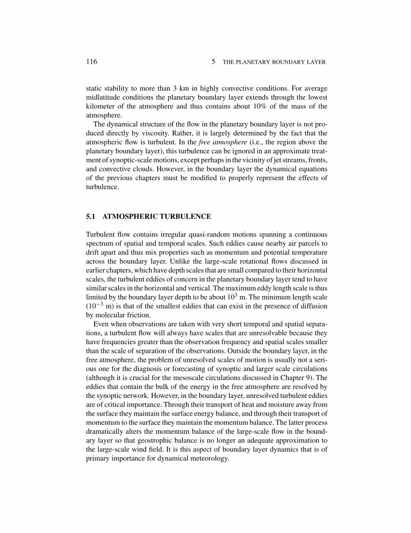
static stability to more than 3 km in highly convective conditions. For averagemidlatitude conditions the planetary boundary layer extends through the lowestkilometer of the atmosphere and thus contains about 10% of the mass of theatmosphere.
The dynamical structure of the flow in the planetary boundary layer is not pro-duced directly by viscosity. Rather, it is largely determined by the fact that theatmospheric flow is turbulent. In the free atmosphere (i.e., the region above theplanetary boundary layer), this turbulence can be ignored in an approximate treat-ment of synoptic-scale motions, except perhaps in the vicinity of jet streams, fronts,and convective clouds. However, in the boundary layer the dynamical equationsof the previous chapters must be modified to properly represent the effects ofturbulence.
5.1 ATMOSPHERIC TURBULENCE
Turbulent flow contains irregular quasi-random motions spanning a continuousspectrum of spatial and temporal scales. Such eddies cause nearby air parcels todrift apart and thus mix properties such as momentum and potential temperatureacross the boundary layer. Unlike the large-scale rotational flows discussed inearlier chapters, which have depth scales that are small compared to their horizontalscales, the turbulent eddies of concern in the planetary boundary layer tend to havesimilar scales in the horizontal and vertical. The maximum eddy length scale is thuslimited by the boundary layer depth to be about 103 m. The minimum length scale(10−3 m) is that of the smallest eddies that can exist in the presence of diffusionby molecular friction.
Even when observations are taken with very short temporal and spatial separa-tions, a turbulent flow will always have scales that are unresolvable because theyhave frequencies greater than the observation frequency and spatial scales smallerthan the scale of separation of the observations. Outside the boundary layer, in thefree atmosphere, the problem of unresolved scales of motion is usually not a seri-ous one for the diagnosis or forecasting of synoptic and larger scale circulations(although it is crucial for the mesoscale circulations discussed in Chapter 9). Theeddies that contain the bulk of the energy in the free atmosphere are resolved bythe synoptic network. However, in the boundary layer, unresolved turbulent eddiesare of critical importance. Through their transport of heat and moisture away fromthe surface they maintain the surface energy balance, and through their transport ofmomentum to the surface they maintain the momentum balance. The latter processdramatically alters the momentum balance of the large-scale flow in the bound-ary layer so that geostrophic balance is no longer an adequate approximation tothe large-scale wind field. It is this aspect of boundary layer dynamics that is ofprimary importance for dynamical meteorology.
January 27, 2004 9:4 Elsevier/AID aid
5.1 atmospheric turbulence 117
5.1.1 The Boussinesq Approximation
The basic state (standard atmosphere) density varies across the lowest kilometer ofthe atmosphere by only about 10%, and the fluctuating component of density devi-ates from the basic state by only a few percentage points. These circumstancesmight suggest that boundary layer dynamics could be modeled by setting den-sity constant and using the theory of homogeneous incompressible fluids. This is,however, generally not the case. Density fluctuations cannot be totally neglectedbecause they are essential for representing the buoyancy force (see the discussionin Section 2.7.3).
Nevertheless, it is still possible to make some important simplifications indynamical equations for application in the boundary layer. The Boussinesq approx-imation is a form of the dynamical equations that is valid for this situation. In thisapproximation, density is replaced by a constant mean value,ρ0, everywhere exceptin the buoyancy term in the vertical momentum equation. The horizontal momen-tum equations (2.24) and (2.25) can then be expressed in Cartesian coordinates as
Du
Dt= − 1
ρ0
∂p
∂x+ f v + Frx (5.1)
andDv
Dt= − 1
ρ0
∂p
∂y− f u + Fry (5.2)
while, with the aid of (2.28) and (2.51) the vertical momentum equation becomes
Dw
Dt= − 1
ρ0
∂p
∂z+ g
θ
θ0+ Frz (5.3)
Here, as in Section 2.7.3, θ designates the departure of potential temperature fromits basic state value θ0(z).1 Thus, the total potential temperature field is given byθtot = θ(x, y, z, t)+ θ0(z), and the adiabatic thermodynamic energy equation hasthe form of (2.54):
Dθ
Dt= −w
dθ0
dz(5.4)
Finally, the continuity equation (2.34) under the Boussinesq approximation is
∂u
∂x+ ∂v
∂y+ ∂w
∂z= 0 (5.5)
1 The reason that we have not used the notation θ ′ to designate the fluctuating part of the potentialtemperature field will become apparent in Section 5.1.2.
January 27, 2004 9:4 Elsevier/AID aid
118 5 the planetary boundary layer
5.1.2 Reynolds Averaging
In a turbulent fluid, a field variable such as velocity measured at a point generallyfluctuates rapidly in time as eddies of various scales pass the point. In order thatmeasurements be truly representative of the large-scale flow, it is necessary toaverage the flow over an interval of time long enough to average out small-scaleeddy fluctuations, but still short enough to preserve the trends in the large-scaleflow field. To do this we assume that the field variables can be separated intoslowly varying mean fields and rapidly varying turbulent components. Followingthe scheme introduced by Reynolds, we then assume that for any field variables,w and θ , for example, the corresponding means are indicated by overbars and thefluctuating components by primes. Thus, w = w+w′ and θ = θ+θ ′. By definition,the means of the fluctuating components vanish; the product of a deviation with amean also vanishes when the time average is applied. Thus,
w′θ = w′ θ = 0
where we have used the fact that a mean variable is constant over the period ofaveraging. The average of the product of deviation components (called the covari-ance) does not generally vanish. Thus, for example, if on average the turbulentvertical velocity is upward where the potential temperature deviation is positiveand downward where it is negative, the product w′θ ′ is positive and the variablesare said to be correlated positively. These averaging rules imply that the averageof the product of two variables will be the product of the average of the means plusthe product of the average of the deviations:
wθ = (w + w′)(θ + θ ′) = wθ + w′θ ′
Before applying the Reynolds decomposition to (5.1)–(5.4), it is convenient torewrite the total derivatives in each equation in flux form. For example, the termon the left in (5.1) may be manipulated with the aid of the continuity equation (5.5)and the chain rule of differentiation to yield
Du
Dt= ∂u
∂t+ u
∂u
∂x+ v
∂u
∂y+ w
∂u
∂z+ u
!∂u
∂x+ ∂v
∂y+ ∂w
∂z
"
= ∂u
∂t+ ∂u2
∂x+ ∂uv
∂y+ ∂uw
∂z(5.6)
Separating each dependent variable into mean and fluctuating parts, substitutinginto (5.6), and averaging then yields
Du
Dt= ∂u
∂t+ ∂
∂x
#uu + u′u′
$+ ∂
∂y
#uv + u′v′
$+ ∂
∂z
#uw + u′w′
$(5.7)
January 27, 2004 9:4 Elsevier/AID aid
5.1 atmospheric turbulence 119
Noting that the mean velocity fields satisfy the continuity equation (5.5), we canrewrite (5.7), as
Du
Dt= Du
Dt+ ∂
∂x
#u′u′
$+ ∂
∂y
#u′v′
$+ ∂
∂z
#u′w′
$(5.8)
whereD
Dt= ∂
∂t+ u
∂
∂x+ v
∂
∂y+ w
∂
∂z
is the rate of change following the mean motion.The mean equations thus have the form
Du
Dt= − 1
ρ0
∂p
∂x+ f v −
%∂u′u′
∂x+ ∂u′v′
∂y+ ∂u′w′
∂z
&
+ Frx (5.9)
Dv
Dt= − 1
ρ0
∂p
∂y− f u −
%∂u′v′
∂x+ ∂v′v′
∂y+ ∂v′w′
∂z
&
+ Fry (5.10)
Dw
Dt= − 1
ρ0
∂p
∂z+ g
θ
θ0−%∂u′w′
∂x+ ∂v′w′
∂y+ ∂w′w′
∂z
&
+ Frz (5.11)
Dθ
Dt= −w
dθ0
dz−%∂u′θ ′
∂x+ ∂v′θ ′
∂y+ ∂w′θ ′
∂z
&
(5.12)
∂u
∂x+ ∂ v
∂y+ ∂w
∂z= 0 (5.13)
The various covariance terms in square brackets in (5.9)–(5.12) represent turbu-lent fluxes. For example, w′θ ′ is a vertical turbulent heat flux in kinematic form.Similarly w′u′ = u′w′ is a vertical turbulent flux of zonal momentum. For manyboundary layers the magnitudes of the turbulent flux divergence terms are of thesame order as the other terms in (5.9)–(5.12). In such cases, it is not possible toneglect the turbulent flux terms even when only the mean flow is of direct interest.Outside the boundary layer the turbulent fluxes are often sufficiently weak so thatthe terms in square brackets in (5.9)–(5.12) can be neglected in the analysis oflarge-scale flows. This assumption was implicitly made in Chapters 3 and 4.
The complete equations for the mean flow (5.9)–(5.13), unlike the equations forthe total flow (5.1)–(5.5), and the approximate equations of Chapters 3 and 4, arenot a closed set, as in addition to the five unknown mean variables u, v, w, θ , p,
there are unknown turbulent fluxes. To solve these equations, closure assump-tions must be made to approximate the unknown fluxes in terms of the fiveknown mean state variables. Away from regions with horizontal inhomogeneities
January 27, 2004 9:4 Elsevier/AID aid
120 5 the planetary boundary layer
(e.g., shorelines, towns, forest edges), we can simplify by assuming that the tur-bulent fluxes are horizontally homogeneous so that it is possible to neglect thehorizontal derivative terms in square brackets in comparison to the terms involvingvertical differentiation.
5.2 TURBULENT KINETIC ENERGY
Vortex stretching and twisting associated with turbulent eddies always tend tocause turbulent energy to flow toward the smallest scales, where it is dissipatedby viscous diffusion. Thus, there must be continuing production of turbulence ifthe turbulent kinetic energy is to remain statistically steady. The primary sourceof boundary layer turbulence depends critically on the structure of the wind andtemperature profiles near the surface. If the lapse rate is unstable, boundary layerturbulence is convectively generated. If it is stable, then instability associated withwind shear must be responsible for generating turbulence in the boundary layer.The comparative roles of these processes can best be understood by examining thebudget for turbulent kinetic energy.
To investigate the production of turbulence, we subtract the component meanmomentum equations (5.9)–(5.11) from the corresponding unaveraged equations(5.1)–(5.3). We then multiply the results by u′, v′, w′, respectively, add the resultingthree equations, and average to obtain the turbulent kinetic energy equation. Thecomplete statement of this equation is quite complicated, but its essence can beexpressed symbolically as
D (T KE)
Dt= MP + BP L + T R − ε (5.14)
where T KE ≡ (u′2 + v′2 + w′2)/2 is the turbulent kinetic energy per unit mass,MP is the mechanical production, BPL is the buoyant production or loss, TR des-ignates redistribution by transport and pressure forces, and ε designates frictionaldissipation. ε is always positive, reflecting the dissipation of the smallest scales ofturbulence by molecular viscosity.
The buoyancy term in (5.14) represents a conversion of energy between meanflow potential energy and turbulent kinetic energy. It is positive for motions thatlower the center of mass of the atmosphere and negative for motions that raise it.The buoyancy term has the form2
BP L ≡ w′θ ′ 'g(θ0)
2 In practice, buoyancy in the boundary layer is modified by the presence of water vapor, which has adensity significantly lower than that of dry air. The potential temperature should be replaced by virtualpotential temperature in (5.14) in order to include this effect. (See, for example, Curry and Webster,1999, p.67.)

January 27, 2004 9:4 Elsevier/AID aid
5.2 turbulent kinetic energy 121
Fig. 5.1 Correlation between vertical velocity and potential temperature perturbations for upward ordownward parcel displacements when the mean potential temperature θ0(z) decreases withheight.
Positive buoyancy production occurs when there is heating at the surface so thatan unstable temperature lapse rate (see Section 2.7.2) develops near the groundand spontaneous convective overturning can occur. As shown in the schematic ofFig. 5.1, convective eddies have positively correlated vertical velocity and potentialtemperature fluctuations and hence provide a source of turbulent kinetic energy andpositive heat flux. This is the dominant source in a convectively unstable boundarylayer. For a statically stable atmosphere, BPL is negative, which tends to reduceor eliminate turbulence.
For both statically stable and unstable boundary layers, turbulence can be gen-erated mechanically by dynamical instability due to wind shear. This process isrepresented by the mechanical production term in (5.14), which represents a con-version of energy between mean flow and turbulent fluctuations. This term isproportional to the shear in the mean flow and has the form
MP ≡ −u′w′ ∂u
∂z− v′w′ ∂ v
∂z(5.15)
MP is positive when the momentum flux is directed down the gradient of themean momentum. Thus, if the mean vertical shear near the surface is westerly(∂u
(∂z > 0), then u′w′ < 0 for MP > 0.
In a statically stable layer, turbulence can exist only if mechanical production islarge enough to overcome the damping effects of stability and viscous dissipation.
January 27, 2004 9:4 Elsevier/AID aid
122 5 the planetary boundary layer
This condition is measured by a quantity called the flux Richardson number. It isdefined as
Rf ≡ −BP L/MP
If the boundary layer is statically unstable, then Rf < 0 and turbulence is sus-tained by convection. For stable conditions, Rf will be greater than zero. Observa-tions suggest that only when Rf is less than about 0.25 (i.e., mechanical productionexceeds buoyancy damping by a factor of 4) is the mechanical production intenseenough to sustain turbulence in a stable layer. Since MP depends on the shear, italways becomes large close enough to the surface. However, as the static stabilityincreases, the depth of the layer in which there is net production of turbulenceshrinks. Thus, when there is a strong temperature inversion, such as produced bynocturnal radiative cooling, the boundary layer depth may be only a few decame-ters, and vertical mixing is strongly suppressed.
5.3 PLANETARY BOUNDARY LAYER MOMENTUM EQUATIONS
For the special case of horizontally homogeneous turbulence above the viscoussublayer, molecular viscosity and horizontal turbulent momentum flux divergenceterms can be neglected. The mean flow horizontal momentum equations (5.9) and(5.10) then become
Du
Dt= − 1
ρ0
∂p
∂x+ f v − ∂u′w′
∂z(5.16)
Dv
Dt= − 1
ρ0
∂p
∂y− f u − ∂v′w′
∂z(5.17)
In general, (5.16) and (5.17) can only be solved for u and v if the vertical distributionof the turbulent momentum flux is known. Because this depends on the structureof the turbulence, no general solution is possible. Rather, a number of approximatesemiempirical methods are used.
For midlatitude synoptic-scale motions, Section 2.4 showed that to a first approx-imation the inertial acceleration terms [the terms on the left in (5.16) and (5.17)]could be neglected compared to the Coriolis force and pressure gradient forceterms. Outside the boundary layer, the resulting approximation was then simplygeostrophic balance. In the boundary layer the inertial terms are still small com-pared to the Coriolis force and pressure gradient force terms, but the turbulentflux terms must be included. Thus, to a first approximation, planetary boundarylayer equations express a three-way balance among the Coriolis force, the pressuregradient force, and the turbulent momentum flux divergence:
f'v − vg
)− ∂u′w′
∂z= 0 (5.18)
January 27, 2004 9:4 Elsevier/AID aid
5.3 planetary boundary layer momentum equations 123
−f'u − ug
)− ∂v′w′
∂z= 0 (5.19)
where (2.23) is used to express the pressure gradient force in terms of geostrophicvelocity.
5.3.1 Well-Mixed Boundary Layer
If a convective boundary layer is topped by a stable layer, turbulent mixing canlead to formation of a well-mixed layer. Such boundary layers occur commonlyover land during the day when surface heating is strong and over oceans when theair near the sea surface is colder than the surface water temperature. The tropicaloceans typically have boundary layers of this type.
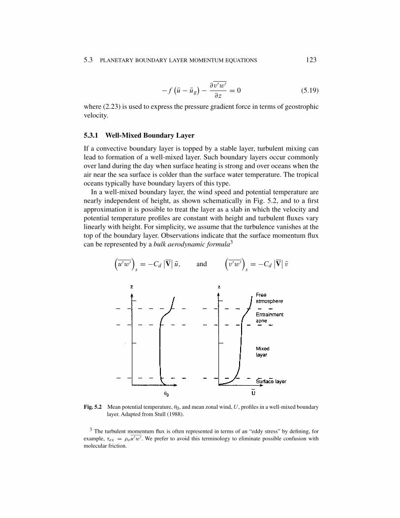
In a well-mixed boundary layer, the wind speed and potential temperature arenearly independent of height, as shown schematically in Fig. 5.2, and to a firstapproximation it is possible to treat the layer as a slab in which the velocity andpotential temperature profiles are constant with height and turbulent fluxes varylinearly with height. For simplicity, we assume that the turbulence vanishes at thetop of the boundary layer. Observations indicate that the surface momentum fluxcan be represented by a bulk aerodynamic formula3
#u′w′
$
s= −Cd
**V** u, and
#v′w′
$
s= −Cd
**V** v
Fig. 5.2 Mean potential temperature, θ0, and mean zonal wind, U , profiles in a well-mixed boundarylayer. Adapted from Stull (1988).
3 The turbulent momentum flux is often represented in terms of an “eddy stress” by defining, forexample, τex = ρou′w′. We prefer to avoid this terminology to eliminate possible confusion withmolecular friction.
January 27, 2004 9:4 Elsevier/AID aid
124 5 the planetary boundary layer
where Cd is a nondimensional drag coefficient, |V| = (u2 + v2)1/2, and thesubscript s denotes surface values (referred to the standard anemometer height).Observations show that Cd is of order 1.5 ×10⁻³ over oceans, but may be severaltimes as large over rough ground.
The approximate planetary boundary layer equations (5.18) and (5.19) can thenbe integrated from the surface to the top of the boundary layer at z = h to give
f'v − vg
)= −
#u′w′
$
s
(h = Cd
**V** u(
h (5.20)
−f'u − ug
)= −
#v′w′
$
s
(h = Cd
**V** v(
h (5.21)
Without loss of generality we can choose axes such that vg = 0. Then (5.20) and(5.21) can be rewritten as
v = κs
**V** u; u = ug − κs
**V** v; (5.22)
where κs ≡ Cd
((f h) . Thus, in the mixed layer the wind speed is less than
the geostrophic speed and there is a component of motion directed toward lowerpressure (i.e., to the left of the geostrophic wind in the Northern Hemisphere andto the right in the Southern Hemisphere) whose magnitude depends on κs . Forexample, if ug = 10 m s–1 and κs = 0.05 m–1 s, then u = 8.28 m s–1, v = 3.77m s–1, and
**V** = 9.10 m s–1 at all heights within this idealized slab mixed layer.
It is the work done by the flow toward lower pressure that balances the frictionaldissipation at the surface. Because boundary layer turbulence tends to reduce windspeeds, the turbulent momentum flux terms are often referred to as boundary layerfriction. It should be kept in mind, however, that the forces involved are due toturbulence, not molecular viscosity.
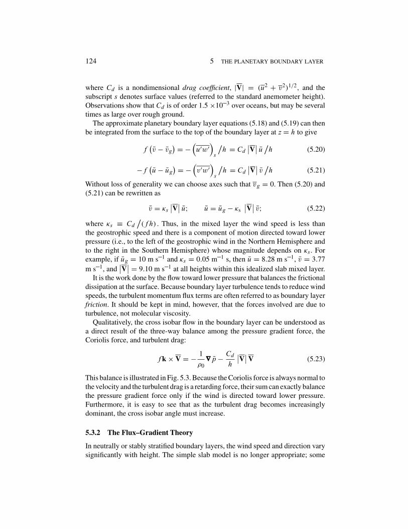
Qualitatively, the cross isobar flow in the boundary layer can be understood asa direct result of the three-way balance among the pressure gradient force, theCoriolis force, and turbulent drag:
f k × V = − 1ρ0
∇p − Cd
h
**V**V (5.23)
This balance is illustrated in Fig. 5.3. Because the Coriolis force is always normal tothe velocity and the turbulent drag is a retarding force, their sum can exactly balancethe pressure gradient force only if the wind is directed toward lower pressure.Furthermore, it is easy to see that as the turbulent drag becomes increasinglydominant, the cross isobar angle must increase.
5.3.2 The Flux–Gradient Theory
In neutrally or stably stratified boundary layers, the wind speed and direction varysignificantly with height. The simple slab model is no longer appropriate; some
January 27, 2004 9:4 Elsevier/AID aid
5.3 planetary boundary layer momentum equations 125
Fig. 5.3 Balance of forces in the well-mixed planetary boundary layer: P designates the pressuregradient force, Co the Coriolis force, and FT the turbulent drag.
means is needed to determine the vertical dependence of the turbulent momentumflux divergence in terms of mean variables in order to obtain closed equations forthe boundary layer variables. The traditional approach to this closure problem isto assume that turbulent eddies act in a manner analogous to molecular diffusionso that the flux of a given field is proportional to the local gradient of the mean. Inthis case the turbulent flux terms in (5.18) and (5.19) are written as
u′w′ = −Km
!∂u
∂z
"; v′w′ = −Km
!∂ v
∂z
"
and the potential temperature flux can be written as
θ ′w′ = −Kh
!∂θ
∂z
"
where Km(m2s−1) is the eddy viscosity coefficient and Khis the eddy diffusivityof heat. This closure scheme is often referred to as K theory.
The K theory has many limitations. Unlike the molecular viscosity coefficient,eddy viscosities depend on the flow rather than the physical properties of thefluid and must be determined empirically for each situation. The simplest modelshave assumed that the eddy exchange coefficient is constant throughout the flow.This approximation may be adequate for estimating the small-scale diffusion ofpassive tracers in the free atmosphere. However, it is a very poor approximationin the boundary layer where the scales and intensities of typical turbulent eddiesare strongly dependent on the distance to the surface as well as the static stability.Furthermore, in many cases the most energetic eddies have dimensions comparableto the boundary layer depth, and neither the momentum flux nor the heat flux isproportional to the local gradient of the mean. For example, in much of the mixedlayer, heat fluxes are positive even though the mean stratification may be very closeto neutral.
January 27, 2004 9:4 Elsevier/AID aid
126 5 the planetary boundary layer
5.3.3 The Mixing Length Hypothesis
The simplest approach to determining a suitable model for the eddy diffusion coef-ficient in the boundary layer is based on the mixing length hypothesis introducedby the famous fluid dynamicist L. Prandtl. This hypothesis assumes that a parcelof fluid displaced vertically will carry the mean properties of its original level fora characteristic distance ξ ′ and then will mix with its surroundings just as an aver-age molecule travels a mean free path before colliding and exchanging momentumwith another molecule. By further analogy to the molecular mechanism, this dis-placement is postulated to create a turbulent fluctuation whose magnitude dependson ξ ′ and the gradient of the mean property. For example,
θ ′ = −ξ ′ ∂θ∂z
; u′ = −ξ ′ ∂u
∂z; v′ = −ξ ′ ∂ v
∂z
where it must be understood that ξ ′ > 0 for upward parcel displacement and ξ ′ < 0for downward parcel displacement. For a conservative property, such as potentialtemperature, this hypothesis is reasonable provided that the eddy scales are smallcompared to the mean flow scale or that the mean gradient is constant with height.However, the hypothesis is less justified in the case of velocity, as pressure gradientforces may cause substantial changes in the velocity during an eddy displacement.
Nevertheless, if we use the mixing length hypothesis, the vertical turbulent fluxof zonal momentum can be written as
−u′w′ = w′ξ ′ ∂u
∂z(5.24)
with analogous expressions for the momentum flux in the meridional directionand the potential temperature flux. In order to estimate w′ in terms of mean fields,we assume that the vertical stability of the atmosphere is nearly neutral so thatbuoyancy effects are small. The horizontal scale of the eddies should then becomparable to the vertical scale so that |w′| ∼ |V′| and we can set
w′ ≈ ξ ′*****∂V∂z
*****
where V′ and V designate the turbulent and mean parts of the horizontal velocityfield, respectively. Here the absolute value of the mean velocity gradient is neededbecause if ξ ′ > 0, then w > 0 (i.e., upward parcel displacements are associatedwith upward eddy velocities). Thus the momentum flux can be written
−u′w′ = ξ ′2*****∂V∂z
*****∂u
∂z= Km
∂u
∂z(5.25)

January 27, 2004 9:4 Elsevier/AID aid
5.3 planetary boundary layer momentum equations 127
where the eddy viscosity is now defined as Km = ξ ′2 **∂V(∂z** = ℓ2
**∂V(∂z**
and the mixing length,
ℓ ≡#ξ ′2$1/2
is the root mean square parcel displacement, which is a measure of average eddysize. This result suggests that larger eddies and greater shears induce greater tur-bulent mixing.
5.3.4 The Ekman Layer
If the flux-gradient approximation is used to represent the turbulent momentumflux divergence terms in (5.18) and (5.19), and the value of Km is taken to beconstant, we obtain the equations of the classical Ekman layer:
Km∂2u
∂z2 + f'v − vg
)= 0 (5.26)
Km∂2v
∂z2 − f'u − ug
)= 0 (5.27)
where we have omitted the overbars because all fields are Reynolds averaged.The Ekman layer equations (5.26) and (5.27) can be solved to determine the
height dependence of the departure of the wind field in the boundary layer fromgeostrophic balance. In order to keep the analysis as simple as possible, we assumethat these equations apply throughout the depth of the boundary layer. The bound-ary conditions on u and v then require that both horizontal velocity componentsvanish at the ground and approach their geostrophic values far from the ground:
u = 0, v = 0 at z = 0u → ug , v → vg as z → ∞ (5.28)
To solve (5.26) and (5.27), we combine them into a single equation by first mul-tiplying (5.27) by i = (−1)1/2 and then adding the result to (5.26) to obtain asecond-order equation in the complex velocity, (u + iv):
Km∂2 (u + iv)
∂z2 − if (u + iv) = −if'ug + ivg
)(5.29)
For simplicity, we assume that the geostrophic wind is independent of height andthat the flow is oriented so that the geostrophic wind is in the zonal direction(vg = 0). Then the general solution of (5.29) is
(u + iv) = A exp+(if/Km)1/2 z
,+ B exp
+− (if/Km)1/2 z
,+ ug (5.30)
January 27, 2004 9:4 Elsevier/AID aid
128 5 the planetary boundary layer
It can be shown that√
i = (1 + i) /√
2. Using this relationship and applying theboundary conditions of (5.28), we find that for the Northern Hemisphere (f > 0),A = 0 and B = −ug. Thus
u + iv = −ug exp-−γ (1 + i) z
.+ ug
where γ = (f/2Km)1/2.Applying the Euler formula exp(−iθ) = cos θ − isin θ and separating the real
from the imaginary part, we obtain for the Northern Hemisphere
u = ug
'1 − e−γ z cos γ z
), v = uge−γ z sin γ z (5.31)
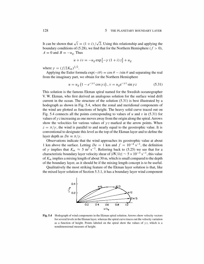
This solution is the famous Ekman spiral named for the Swedish oceanographerV. W. Ekman, who first derived an analogous solution for the surface wind driftcurrent in the ocean. The structure of the solution (5.31) is best illustrated by ahodograph as shown in Fig. 5.4, where the zonal and meridional components ofthe wind are plotted as functions of height. The heavy solid curve traced out onFig. 5.4 connects all the points corresponding to values of u and v in (5.31) forvalues of γ z increasing as one moves away from the origin along the spiral.Arrowsshow the velocities for various values of γ z marked at the arrow points. Whenz = π/γ , the wind is parallel to and nearly equal to the geostrophic value. It isconventional to designate this level as the top of the Ekman layer and to define thelayer depth as De ≡ π/γ .
Observations indicate that the wind approaches its geostrophic value at about1 km above the surface. Letting De = 1 km and f = 10−4 s−1, the definitionof γ implies that Km ≈ 5 m2 s−1. Referring back to (5.25) we see that for acharacteristic boundary layer velocity shear of |δV/δz| ∼ 5×10⁻³ s−1, this valueof Km implies a mixing length of about 30 m, which is small compared to the depthof the boundary layer, as it should be if the mixing length concept is to be useful.
Qualitatively the most striking feature of the Ekman layer solution is that, likethe mixed layer solution of Section 5.3.1, it has a boundary layer wind component
Fig. 5.4 Hodograph of wind components in the Ekman spiral solution. Arrows show velocity vectorsfor several levels in the Ekman layer, whereas the spiral curve traces out the velocity variationas a function of height. Points labeled on the spiral show the values of γ z, which is anondimensional measure of height.
January 27, 2004 9:4 Elsevier/AID aid
5.3 planetary boundary layer momentum equations 129
directed toward lower pressure. As in the mixed layer case, this is a direct result ofthe three-way balance among the pressure gradient force, the Coriolis force, andthe turbulent drag.
The ideal Ekman layer discussed here is rarely, if ever, observed in the atmo-spheric boundary layer. Partly this is because turbulent momentum fluxes are usu-ally not simply proportional to the gradient of the mean momentum. However,even if the flux–gradient model were correct, it still would not be proper to assumea constant eddy viscosity coefficient, as in reality Km must vary rapidly with heightnear the ground. Thus, the Ekman layer solution should not be carried all the wayto the surface.
5.3.5 The Surface Layer
Some of the inadequacies of the Ekman layer model can be overcome if we dis-tinguish a surface layer from the remainder of the planetary boundary layer. Thesurface layer, whose depth depends on stability, but is usually less than 10% of thetotal boundary layer depth, is maintained entirely by vertical momentum transferby the turbulent eddies; it is not directly dependent on the Coriolis or pressure gra-dient forces. Analysis is facilitated by supposing that the wind close to the surfaceis directed parallel to the x axis. The kinematic turbulent momentum flux can thenbe expressed in terms of a friction velocity, u∗, which is defined as4
u2∗ ≡
***(u′w′)s
***
Measurements indicate that the magnitude of the surface momentum flux is ofthe order 0.1 m2 s−2. Thus the friction velocity is typically of the order 0.3 m s−1.
According to the scale analysis in Section 2.4, the Coriolis and pressure gradientforce terms in (5.16) have magnitudes of about 10−3 m s−2 in midlatitudes. Themomentum flux divergence in the surface layer cannot exceed this magnitude orit would be unbalanced. Thus, it is necessary that
δ'u2
∗)
δz≤ 10−3 m s−2
For δz = 10 m, this implies that δ(u2∗) ≤ 10−2 m2 s−2, so that the change in the
vertical momentum flux in the lowest 10 m of the atmosphere is less than 10% ofthe surface flux. To a first approximation it is then permissible to assume that inthe lowest several meters of the atmosphere the turbulent flux remains constant atits surface value, so that with the aid of (5.25)
Km∂u
∂z= u2
∗ (5.32)
4 Thus the surface eddy stress (see footnote 3) is equal to ρ0u2∗.
January 27, 2004 9:4 Elsevier/AID aid
130 5 the planetary boundary layer
where we have parameterized the surface momentum flux in terms of the eddyviscosity coefficient. In applying Km in the Ekman layer solution, we assumed aconstant value throughout the boundary layer. Near the surface, however, the verti-cal eddy scale is limited by the distance to the surface. Thus, a logical choice for themixing length is ℓ = kz where k is a constant. In that case Km = (kz)2
**∂u(∂z**.
Substituting this expression into (5.32) and taking the square root of the resultgives
∂u(∂z = u∗/(kz) (5.33)
Integrating with respect to z yields the logarithmic wind profile
u ='u∗(
k)
ln'z(
z0)
(5.34)
where z0, the roughness length, is a constant of integration chosen so that u = 0at z = z0. The constant k in (5.34) is a universal constant called von Karman’sconstant, which has an experimentally determined value of k ≈ 0.4. The roughnesslength z0 varies widely depending on the physical characteristics of the surface.For grassy fields, typical values are in the range of 1−4 cm. Although a number ofassumptions are required in the derivation of (5.34), many experimental programshave shown that the logarithmic profile provides a generally satisfactory fit toobserved wind profiles in the surface layer.
5.3.6 The Modified Ekman Layer
As pointed out earlier, the Ekman layer solution is not applicable in the surfacelayer. A more satisfactory representation for the planetary boundary layer can beobtained by combining the logarithmic surface layer profile with the Ekman spiral.In this approach the eddy viscosity coefficient is again treated as a constant, but(5.29) is applied only to the region above the surface layer and the velocity andshear at the bottom of the Ekman layer are matched to those at the top of thesurface layer. The resulting modified Ekman spiral provides a somewhat better fitto observations than the classical Ekman spiral. However, observed winds in theplanetary boundary layer generally deviate substantially from the spiral pattern.Both transience and baroclinic effects (i.e., vertical shear of the geostrophic wind inthe boundary layer) may cause deviations from the Ekman solution. However, evenin steady-state barotropic situations with near neutral static stability, the Ekmanspiral is seldom observed.
It turns out that the Ekman layer wind profile is generally unstable for a neutrallybuoyant atmosphere. The circulations that develop as a result of this instability havehorizontal and vertical scales comparable to the depth of the boundary layer. Thus,it is not possible to parameterize them by a simple flux–gradient relationship. How-ever, these circulations do in general transport considerable momentum vertically.The net result is usually to decrease the angle between the boundary layer wind
January 27, 2004 9:4 Elsevier/AID aid
5.4 secondary circulations and spin down 131
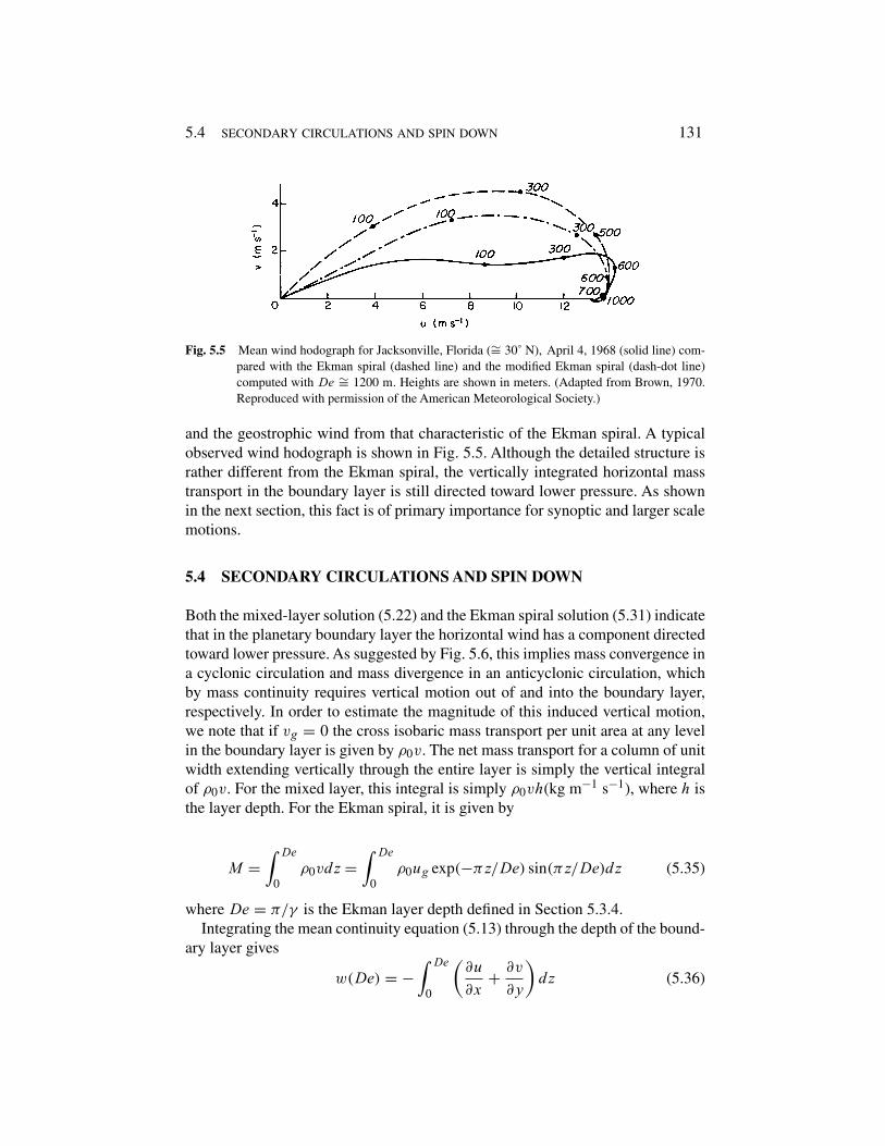
Fig. 5.5 Mean wind hodograph for Jacksonville, Florida (∼= 30˚ N), April 4, 1968 (solid line) com-pared with the Ekman spiral (dashed line) and the modified Ekman spiral (dash-dot line)computed with De ∼= 1200 m. Heights are shown in meters. (Adapted from Brown, 1970.Reproduced with permission of the American Meteorological Society.)
and the geostrophic wind from that characteristic of the Ekman spiral. A typicalobserved wind hodograph is shown in Fig. 5.5. Although the detailed structure israther different from the Ekman spiral, the vertically integrated horizontal masstransport in the boundary layer is still directed toward lower pressure. As shownin the next section, this fact is of primary importance for synoptic and larger scalemotions.
5.4 SECONDARY CIRCULATIONS AND SPIN DOWN
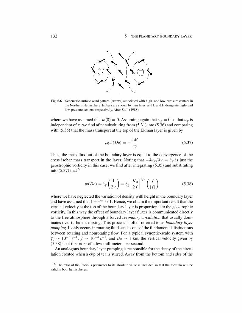
Both the mixed-layer solution (5.22) and the Ekman spiral solution (5.31) indicatethat in the planetary boundary layer the horizontal wind has a component directedtoward lower pressure. As suggested by Fig. 5.6, this implies mass convergence ina cyclonic circulation and mass divergence in an anticyclonic circulation, whichby mass continuity requires vertical motion out of and into the boundary layer,respectively. In order to estimate the magnitude of this induced vertical motion,we note that if vg = 0 the cross isobaric mass transport per unit area at any levelin the boundary layer is given by ρ0v. The net mass transport for a column of unitwidth extending vertically through the entire layer is simply the vertical integralof ρ0v. For the mixed layer, this integral is simply ρ0vh(kg m−1 s−1), where h isthe layer depth. For the Ekman spiral, it is given by
M =/ De
0ρ0vdz =
/ De
0ρ0ug exp(−πz/De) sin(πz/De)dz (5.35)
where De = π/γ is the Ekman layer depth defined in Section 5.3.4.Integrating the mean continuity equation (5.13) through the depth of the bound-
ary layer gives
w(De) = −/ De
0
!∂u
∂x+ ∂v
∂y
"dz (5.36)
January 27, 2004 9:4 Elsevier/AID aid
132 5 the planetary boundary layer
Fig. 5.6 Schematic surface wind pattern (arrows) associated with high- and low-pressure centers inthe Northern Hemisphere. Isobars are shown by thin lines, and L and H designate high- andlow-pressure centers, respectively. After Stull (1988).
where we have assumed that w(0) = 0. Assuming again that vg = 0 so that ug isindependent of x, we find after substituting from (5.31) into (5.36) and comparingwith (5.35) that the mass transport at the top of the Ekman layer is given by
ρ0w(De) = −∂M
∂y(5.37)
Thus, the mass flux out of the boundary layer is equal to the convergence of thecross isobar mass transport in the layer. Noting that −∂ug/∂y = ζg is just thegeostrophic vorticity in this case, we find after integrating (5.35) and substitutinginto (5.37) that 5
w(De) = ζg
!1
2γ
"= ζg
****Km
2f
****1/2 ! f
|f |
"(5.38)
where we have neglected the variation of density with height in the boundary layerand have assumed that 1 + e-π ≈ 1. Hence, we obtain the important result that thevertical velocity at the top of the boundary layer is proportional to the geostrophicvorticity. In this way the effect of boundary layer fluxes is communicated directlyto the free atmosphere through a forced secondary circulation that usually dom-inates over turbulent mixing. This process is often referred to as boundary layerpumping. It only occurs in rotating fluids and is one of the fundamental distinctionsbetween rotating and nonrotating flow. For a typical synoptic-scale system withζg ∼ 10−5 s−1, f ∼ 10−4 s−1, and De ∼ 1 km, the vertical velocity given by(5.38) is of the order of a few millimeters per second.
An analogous boundary layer pumping is responsible for the decay of the circu-lation created when a cup of tea is stirred. Away from the bottom and sides of the
5 The ratio of the Coriolis parameter to its absolute value is included so that the formula will bevalid in both hemispheres.
January 27, 2004 9:4 Elsevier/AID aid
5.4 secondary circulations and spin down 133
cup there is an approximate balance between the radial pressure gradient and thecentrifugal force of the spinning fluid. However, near the bottom, viscosity slowsthe motion and the centrifugal force is not sufficient to balance the radial pressuregradient. (Note that the radial pressure gradient is independent of depth, as wateris an incompressible fluid.) Therefore, radial inflow takes place near the bottomof the cup. Because of this inflow, the tea leaves always are observed to clusternear the center at the bottom of the cup if the tea has been stirred. By continuity ofmass, the radial inflow in the bottom boundary layer requires upward motion and aslow compensating outward radial flow throughout the remaining depth of the tea.This slow outward radial flow approximately conserves angular momentum, andby replacing high angular momentum fluid by low angular momentum fluid servesto spin down the vorticity in the cup far more rapidly than could mere diffusion.
The characteristic time for the secondary circulation to spin down an atmo-spheric vortex is illustrated most easily in the case of a barotropic atmosphere.For synoptic-scale motions the barotropic vorticity equation (4.24) can be writtenapproximately as
Dζg
Dt= −f
!∂u
∂x+ ∂v
∂y
"= f
∂w
∂z(5.39)
where we have neglected ζg compared to f in the divergence term and have alsoneglected the latitudinal variation of f . Recalling that the geostrophic vorticity isindependent of height in a barotropic atmosphere, (5.39) can be integrated easilyfrom the top of the Ekman layer (z = De) to the tropopause (z = H ) to give
Dζg
Dt= +f
0w(H ) − w(De)
(H − De)
1(5.40)
Substituting for w(De) from (5.38), assuming that w(H ) = 0 and that H ≫ De,(5.40) may be written as
Dζg
Dt= −
****f Km
2H 2
****1/2
ζg (5.41)
This equation may be integrated in time to give
ζg (t) = ζg (0) exp (−t/τe) (5.42)
where ζg(0) is the value of the geostrophic vorticity at time t = 0, and τe ≡H |2/(f Km)|1/2 is the time that it takes the vorticity to decrease to e−1 of itsoriginal value.
This e-folding time scale is referred to as the barotropic spin-down time. Takingtypical values of the parameters as follows: H ≡ 10 km, f = 10−4 s−1, andKm = 10 m2 s−1, we find that τe ≈ 4 days. Thus, for midlatitude synoptic-scaledisturbances in a barotropic atmosphere, the characteristic spin-down time is afew days. This decay time scale should be compared to the time scale for ordinary
January 27, 2004 9:4 Elsevier/AID aid
134 5 the planetary boundary layer
viscous diffusion. For viscous diffusion the time scale can be estimated from scaleanalysis of the diffusion equation
∂u
∂t= Km
∂2u
∂z2 (5.43)
If τd is the diffusive time scale and H is a characteristic vertical scale for diffusion,then from the diffusion equation
U(τd ∼ KmU
2H 2
so that τd ∼ H 2/Km. For the above values of H and Km, the diffusion time scaleis thus about 100 days. Hence, in the absence of convective clouds the spin-downprocess is a far more effective mechanism for destroying vorticity in a rotatingatmosphere than eddy diffusion. Cumulonimbus convection can produce rapidturbulent transports of heat and momentum through the entire depth of the tro-posphere. These must be considered together with boundary layer pumping forintense systems such as hurricanes.
Physically the spin-down process in the atmospheric case is similar to thatdescribed for the teacup, except that in synoptic-scale systems it is primarily theCoriolis force that balances the pressure gradient force away from the boundary,not the centrifugal force. Again the role of the secondary circulation driven byforces resulting from boundary layer drag is to provide a slow radial flow in theinterior that is superposed on the azimuthal circulation of the vortex above theboundary layer. This secondary circulation is directed outward in a cyclone so thatthe horizontal area enclosed by any chain of fluid particles gradually increases.Since the circulation is conserved, the azimuthal velocity at any distance from thevortex center must decrease in time or, from another point of view, the Coriolisforce for the outward-flowing fluid is directed clockwise, and this force thus exertsa torque opposite to the direction of the circulation of the vortex. Fig. 5.7 shows aqualitative sketch of the streamlines of this secondary flow.
It should now be obvious exactly what is meant by the term secondary circula-tion. It is simply a circulation superposed on the primary circulation (in this casethe azimuthal circulation of the vortex) by the physical constraints of the system.In the case of the boundary layer, viscosity is responsible for the presence of thesecondary circulation. However, other processes, such as temperature advectionand diabatic heating, may also lead to secondary circulations, as shown later.
The above discussion has concerned only the neutrally stratified barotropicatmosphere. An analysis for the more realistic case of a stably stratified baroclinicatmosphere is more complicated. However, qualitatively the effects of stratifica-tion may be easily understood. The buoyancy force (see Section 2.7.3) will actto suppress vertical motion, as air lifted vertically in a stable environment will be
January 27, 2004 9:4 Elsevier/AID aid
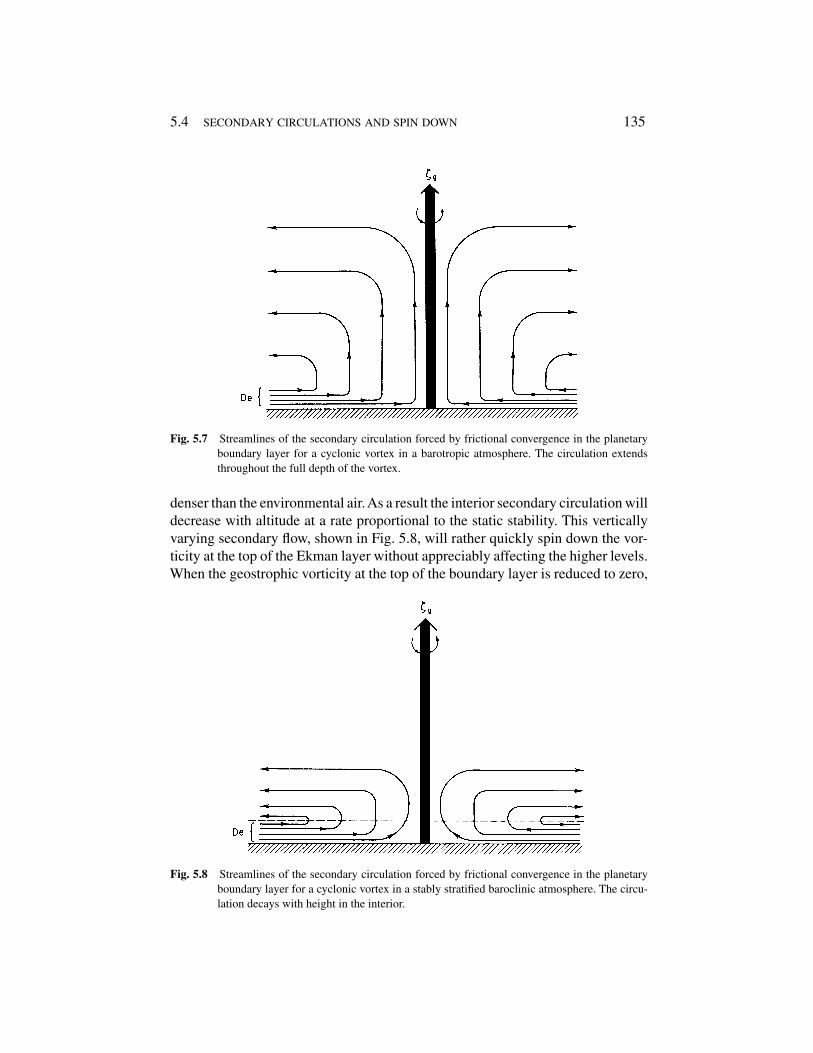
5.4 secondary circulations and spin down 135
Fig. 5.7 Streamlines of the secondary circulation forced by frictional convergence in the planetaryboundary layer for a cyclonic vortex in a barotropic atmosphere. The circulation extendsthroughout the full depth of the vortex.
denser than the environmental air.As a result the interior secondary circulation willdecrease with altitude at a rate proportional to the static stability. This verticallyvarying secondary flow, shown in Fig. 5.8, will rather quickly spin down the vor-ticity at the top of the Ekman layer without appreciably affecting the higher levels.When the geostrophic vorticity at the top of the boundary layer is reduced to zero,
Fig. 5.8 Streamlines of the secondary circulation forced by frictional convergence in the planetaryboundary layer for a cyclonic vortex in a stably stratified baroclinic atmosphere. The circu-lation decays with height in the interior.

January 27, 2004 9:4 Elsevier/AID aid
136 5 the planetary boundary layer
the pumping action of the Ekman layer is eliminated. The result is a baroclinic vor-tex with a vertical shear of the azimuthal velocity that is just strong enough to bringζg to zero at the top of the boundary layer. This vertical shear of the geostrophicwind requires a radial temperature gradient that is in fact produced during thespin-down phase by adiabatic cooling of the air forced out of the Ekman layer.Thus, the secondary circulation in the baroclinic atmosphere serves two purposes:(1) it changes the azimuthal velocity field of the vortex through the action of theCoriolis force and (2) it changes the temperature distribution so that a thermal windbalance is always maintained between the vertical shear of the azimuthal velocityand the radial temperature gradient.
PROBLEMS
5.1. Verify by direct substitution that the Ekman spiral expression (5.31) is indeeda solution of the boundary layer equations (5.26) and (5.27) for the casevg = 0.
5.2. Derive the Ekman spiral solution for the more general case where thegeostrophic wind has both x and y components (ug and vg , respectively),which are independent of height.
5.3. Letting the Coriolis parameter and density be constants, show that (5.38) iscorrect for the more general Ekman spiral solution obtained in Problem 5.2.
5.4. For laminar flow in a rotating cylindrical vessel filled with water (molecularkinematic viscosity ν = 0.01 cm2 s−1), compute the depth of the Ekmanlayer and the spin-down time if the depth of the fluid is 30 cm and the rotationrate of the tank is 10 revolutions per minute. How small would the radius ofthe tank have to be in order that the time scale for viscous diffusion fromthe side walls be comparable to the spin-down time?
5.5. Suppose that at 43˚ N the geostrophic wind is westerly at 15 m s−1. Computethe net cross isobaric transport in the planetary boundary layer using both themixed layer solution (5.22) and the Ekman layer solution (5.31).You may let|V| = ug in (5.22), h = De = 1 km, κs = 0.05 m−1s, and ρ = 1 kg m−3.
5.6. Derive an expression for the wind-driven surface Ekman layer in the ocean.Assume that the wind stress τw is constant and directed along the x axis.The continuity of turbulent momentum flux at the air–sea interface (z = 0)
requires that the wind stress divided by air density must equal the oceanicturbulent momentum flux at z = 0. Thus, if the flux–gradient theory is used,the boundary condition at the surface becomes
ρ0K∂u
∂z= τw, ρ0K
∂v
∂z= 0, at z = 0