Even Faster Accelerated Coordinate Descent Using …proceedings.mlr.press/v48/allen-zhuc16.pdf · Even Faster Accelerated Coordinate Descent Using Non-Uniform Sampling Paper Euclidean

Even Faster Accelerated Coordinate Descent Using Non-Uniform Sampling

Zeyuan Allen-Zhu [email protected]

Princeton University

Zheng Qu [email protected]

University of Hong Kong

Peter Richtarik [email protected]

University of Edinburgh

Yang Yuan [email protected]

Cornell University

AbstractAccelerated coordinate descent is widely used inoptimization due to its cheap per-iteration costand scalability to large-scale problems. Up to aprimal-dual transformation, it is also the same asaccelerated stochastic gradient descent that is oneof the central methods used in machine learning.

In this paper, we improve the best known run-ning time of accelerated coordinate descent bya factor up to

√n. Our improvement is based

on a clean, novel non-uniform sampling that se-lects each coordinate with a probability propor-tional to the square root of its smoothness pa-rameter. Our proof technique also deviates fromthe classical estimation sequence technique usedin prior work. Our speed-up applies to impor-tant problems such as empirical risk minimiza-tion and solving linear systems, both in theoryand in practice.1

1 IntroductionFirst-order methods have received extensive attention in thepast two decades due to their ability to handle large-scaleoptimization problems. Recently, the development of co-ordinate versions of first-order methods have pushed their

1The results of this paper first appeared on arXiv in December2015. In March 2016, Nesterov and Stich independently obtainedour same results in a technical report (Nesterov & Stich, 2016).

The full version of this paper can be found on http://arxiv.org/abs/1512.09103.

Proceedings of the 33 rd International Conference on MachineLearning, New York, NY, USA, 2016. JMLR: W&CP volume48. Copyright 2016 by the author(s).

running times even faster. As a notable example, the state-of-the-art algorithm for empirical risk minimization (ERM)problems, up to a primal-dual transformation, is preciselyaccelerated coordinate descent (Lin et al., 2014).

In this paper, we consider the following unconstrained min-imization problem2

minx∈Rn

f(x) (1.1)

where the objective f : Rn → R is continuously differ-entiable and convex. Below, we assume that f(·) is Li-smooth with respect to its i-th coordinate.

Informally, coordinate smoothness means for each input x,if we add its i-th coordinate by at most δ, the correspond-ing coordinate gradient∇if(x+ δei) differs from∇if(x)by at most Li times |δ|. Under this definition, the larger Liis, the less smooth f is along the ei direction and thereforethe harder it is to minimize f along the ei direction.3 Intu-itively, this implies we should spend more energy (i.e., as-sign more sampling probability) on coordinates with largerLi. However, it was unclear what the best design is for sucha distribution. In this paper, we present a clean and novelnon-uniform sampling method which gives a faster conver-gence rate. Before going into the details, we first draw adistinction between non-accelerated and accelerated coor-dinate descent methods.

Non-Accelerated vs. Accelerated Methods. For smooth2The results of this paper generalize to the so-called proxi-

mal case that is to allow an additional separable term ψ(x)def=∑n

i=1 ψi(xi) to be added. The proofs require some non-trivialchanges so we refrain from doing so in this version of the paper.

3For instance, if the i-th coordinate is selected, mostcoordinate-descent methods are only capable of performing anupdate x′ ← x − 1

Li∇if(x) with step length inversely propor-

tional to Li.

http://arxiv.org/abs/1512.09103

http://arxiv.org/abs/1512.09103


convex minimization, many first-order methods converge ata rate 1/ε to obtain an additive error ε > 0. In 1983, Nes-terov demonstrated that a better and optimal rate 1/

√ε can

be obtained using his seminal accelerated gradient descentmethod. (Nesterov, 1983)

For this reason, people refer to methods converging at rate1/ε as non-accelerated first-order methods, while those atrate 1/

√ε as accelerated first-order methods. Similarly,

when the objective f(·) is known to be strongly convexwith parameter σ > 0, non-accelerated methods convergeat a rate inversely proportional to σ, while accelerated onesconverge at a rate inversely proportional to

√σ. Although

being much faster, accelerated first-order methods are alsomuch more involved to design, see some recent attemptsfor designing accelerated methods in conceptually simplermanners (O’Donoghue & Candes, 2013; Su et al., 2014;Allen-Zhu & Orecchia, 2014; Bubeck et al., 2015).

Such a distinction continues to hold on the coordinate-gradient setting. A coordinate descent method iterativelyselects a coordinate i ∈ [n] at random, and updates the it-erate x according to its coordinate gradient ∇if(x). Aswe shall see later, designing good sampling probabilitiesis well-studied for non-accelerated coordinate descent. Incontrast, less is known in the more challenging acceleratedregime, and we hope our work fills this gap.

We begin describing our result and compare it to the litera-ture in the Euclidean norm case.

1.1 The Standard Euclidean Norm CaseIn the non-accelerated world, in 2012, Nesterov (Nes-terov, 2012) proposed a coordinate descent method calledRCDM, which is a simple adaption of the full gradient de-scent method (see for instance the textbook (Nesterov,2004)). At each iteration, RCDM selects a coordinate iwith probability proportional to Li, and performs updatex′ ← x − 1

Li∇if(x). The number of iterations required

to reach an ε error, denoted by T in this paper, satisfiesT = O(

∑i Liε ‖x0 − x∗‖2) for RCDM. Here, we denote by

x0 the starting vector, x∗ the minimizer of f , and ‖ · ‖ the`2 Euclidean norm.

This convergence rate is usually compared to that of fullgradient descent: if L is the global smoothness parame-ter of f(·), then full gradient descent converges in T =O(Lε ‖x0 − x

∗‖2) iterations. Since Li is never larger thanL, and performing a coordinate descent step is usually ntimes faster than a full gradient step, RCDM performs fasterthan gradient descent in most applications.

In the same paper (Nesterov, 2012), Nesterov also demon-strated the possibility of performing accelerated coordinategradient descent via a simple adaption of its full-gradientvariant (Nesterov, 1983; 2004; 2005). This has been lateranalyzed in full by Lee and Sidford (Lee & Sidford, 2013),

and they named this method accelerated coordinate de-scent method (ACDM). ACDM converges the following num-ber of iterations:

T =

O(√

n∑i Li√ε‖x0 − x∗‖

), when f is convex

O(√

n∑i Li√σ

log 1ε

),

when f is σ-stronglyconvex

ACDM is built upon the estimation sequence technique ofNesterov (Nesterov, 1983; 2004; 2012), and similar toRCDM, ACDM also selects each coordinate i (essentially) witha probability proportional to Li.4 Since the analysis of Leeand Sidford is tight, it has been thought that the iterationbound T is not improvable.

In this paper, with a different non-uniform samplingmethod, we develop a new accelerated coordinate descentmethod NU ACDM that converges in T iterations, where

T =

O(∑

i

√Li√ε‖x0 − x∗‖

), when f is convex

O(∑

i

√Li√σ

log 1ε

),

when f is σ-stronglyconvex

Note that NU ACDM is always faster than ACDM because∑i

√Li ≤

√n∑i Li. In the case when (L1, . . . , Ln)

is non-uniform, our method runs faster by a factor up to√n.5 In our sampling step, we select each coordinate i

with probability exactly proportional to√Li, rather than

(roughly) proportional to Li. Thus, we need a differentanalysis from ACDM (Lee & Sidford, 2013), and also avoidthe more complicated estimation sequence analysis.

1.2 The General Lβ-Norm Case

Define the Lβ norm ‖y‖2Lβdef=∑i L

βi · y2i for β ∈ [0, 1].

Many accelerated coordinate descent methods provide con-vergence guarantees with respect to the L1 norm (Lu &Xiao, 2013; Fercoq & Richtarik, 2015) or the Lβ norm(Nesterov, 2012; Lin et al., 2014; Lee & Sidford, 2013).

For instance, RCDM takes β as an input, and converges inT = O

(S1−βε ‖x0 − x

∗‖2Lβ)

iterations if one samples each

coordinate i with probability L1−βi /S1−β , where Sα

def=∑

i Lαi . In (Lee & Sidford, 2013), Lee and Sidford showed

that their ACDM converges in T iterations with the same

4More precisely, they select each coordinate i with a probabil-ity proportional to maxLi, 1

n

∑j Lj. As a consequence, each

coordinate i is selected with probability at least Ω(1/n). Lee andSidford emphasized that using this sampling method, rather thanchoosing each i directly with probability Li/(

∑j Lj), is essen-

tial for ACDM to obtain the accelerated convergence rate.5If L1 = · · · = Ln, we have

∑i

√Li =

√n∑i Li.

However, if L1 = 1 while L2 = · · · = Ln = 0, we have∑i

√Li = 1√

n·√n∑i Li.


PaperEuclidean β = 0 Case β ∈ [0, 1] Case β = 1 Case

stronglyconvex non strongly convex strongly

convex non strongly convex stronglyconvex non strongly convex

RCDM ,∑i Liσ

log 1ε

∑i Liε‖x0 − x∗‖2

S1−βσβ

log 1ε

S1−βε‖x0 − x∗‖2Lβ

nσ1

log 1ε

nε‖x0 − x∗‖2L1

APCG , RBCD ,Nesterov ,APPROX

- - - - n√σ1

log 1ε

n√ε‖x0 − x∗‖L1

ACDM√n∑i Li√σ

log 1ε

√n∑i Li√

ε/ log 1ε

‖x0−x∗‖√nS1−β√σβ

log 1ε

√nS1−β

√ε/ log 1

ε

‖x0−x∗‖Lβ√n√σ1

log 1ε

n√ε/ log 1

ε

‖x0−x∗‖L1

this paper∑i

√Li√σ

log 1ε

∑i

√Li√ε‖x0 − x∗‖

S(1−β)/2√σβ

log 1ε

S(1−β)/2√ε‖x0−x∗‖Lβ

√n√σ1

log 1ε

n√ε‖x0 − x∗‖L1

Table 1. Comparisons among coordinate descent methods, where Sαdef=∑i L

αi .

sampling probabilities L1−βi /S1−β , where

T =

O(√

nS1−β√ε‖x0 − x∗‖2Lβ

), when f is convex

O(√

nS1−β√σβ

log 1ε

),

when f is σβ-strongly convex w.r.t.the Lβ norm

This is always faster than RCDM. Note that, in the specialcase of β = 1 (and thus using uniform sampling probabili-ties), this same convergence result is also obtained by Nes-terov (Nesterov, 2012), APCG (Lin et al., 2014), RBCD (Lu& Xiao, 2013), and APPROX (Fercoq & Richtarik, 2015).(See Table 1.)

Our method NU ACDM improves this convergence to

T =

O(S(1−β)/2√

ε‖x0 − x∗‖Lβ

), when f is convex

O(S(1−β)/2√

σβlog 1

ε

),

when f is σβ-strongly convex w.r.t.the Lβ norm

Since√S1−β ≤ S(1−β)/2 ≤

√nS1−β , our method

is faster than ACDM by a factor up to√n. Our im-

provement is again due to the new choice of samplingprobabilities —we select each coordinate i with proba-bility L(1−β)/2

i /S(1−β)/2 which is different from RCDM orACDM— as well as our new proof that avoids the use of es-timation sequence.

Remark 1.1. For the strongly convex case, convergenceresults with respect to Euclidean norms are usually morerelevant to applications: for instance, the `2 regularizeris the most common one used in machine learning appli-cations and algorithms designed for the Euclidean normshould be used for a better performance.6 However, in thenon-strongly convex case, results with respect to differentβ are in general incomparable. We include experiments inSection 7.3 to illustrate this.

6In contrast, consider an objective f(x) equipped with a regu-larizer σ

2‖x‖2. Such an objective is also strongly convex with re-

spect to the Lβ norm with parameter mini L−βi . If one applies an

algorithm designed for the Lβ norm using this parameter, the con-vergence would be much worse than the first column of Table 1.

2 ApplicationsEmpirical Risk Minimization. A cornerstone problemin machine learning is empirical risk minimization (ERM).Let a1, . . . , an ∈ Rd be the feature vectors of n data sam-ples, φ1, . . . , φn : R → R be a sequence of convex lossfunctions, and r : Rd → R be a convex function (oftenknown as a regularizer). The goal of ERM problem is tosolve the following primal convex problem:

minw∈Rd P (w)def= 1

n

∑ni=1 φi

(〈ai, w〉

)+ r(w). (2.1)

This includes a family of important problems such as SVM,Lasso, ridge regression, and logistic regression. Lin, Luand Xiao (Lin et al., 2014) showed that the above mini-mization problem is equivalent to the following dual one:

miny∈Rn D(y)def= 1

n

∑ni=1 φ

∗i (yi) + r∗

(− 1n

∑ni=1 yiai

),

(2.2)where φ∗i and r∗ are respectively the Fenchel conjugatefunction of φi and r.7 Most importantly, if properly prepro-cessed, D(y) can be shown to be coordinate-wise smoothand therefore accelerated coordinate descent methods canbe applied to minimize D(y). This approach leads to al-gorithm APCG, which matches the best known worst-caserunning time on solving (2.1) up to a logarithmic factor.8

However, by taking a closer look, the coordinate smooth-ness parameters L1, . . . , Ln of D(y) are data dependent.Indeed, Li is roughly proportional to the Euclidean normsquare of the i-th feature vector. Therefore, we can applyNU ACDM in this paper to improve the running time obtainedby APCG or AccSDCA. This is done in Section 7.

Note that each iteration of NU ACDM selects a feature vectorwith a probability (roughly) proportional to its Euclideannorm. This is very different from the recent work of Zhaoand Zhang (Zhao & Zhang, 2015), where they observedthat for SDCA (Shalev-Shwartz & Zhang, 2013), a non-

7The conjugate of r(x) is r∗(y)def= maxwyTw − r(w).

8Accelerated algorithms for solving (2.1) were first obtainedby AccSDCA (Shalev-Shwartz & Zhang, 2014), and more recentlyimproved by Katyusha (Allen-Zhu, 2016).


accelerated method, feature vectors should be sampled withprobabilities proportional to their Euclidean norm squares.If one also uses the squared norms in the accelerated set-ting, he will only get a running time similar to ACDM, andtherefore worse than our NU ACDM.

We also mention one recent result that uses our NU ACDM todevelop faster ERM methods by exploiting the clusteringstructure of the dataset (Allen-Zhu et al., 2016).

Solving Linear Systems. Consider a linear system Ax =b for some full row rank matrix A ∈ Rm×n where m ≥ n.Denoting ai ∈ Rn as the i-th row vector of matrix A, thecelebrated Kaczmarz method (Kaczmarz, 1937) iterativelypicks one of the row vectors ai and computes

xk+1 ← xk + bi−〈ai,xk〉‖ai‖2 ai .

Although many deterministic schemes have been proposedregarding how to select row vectors, many of them aredifficult to analyze or compare. In a breakthrough paper,Strohmer and Vershynin (Strohmer & Vershynin, 2009) an-alyzed a randomized scheme and proved that:

Theorem 2.1 (Randomized Kaczmarz (Strohmer & Ver-shynin, 2009)). If one samples row i with probability pro-portional to ‖ai‖2 in each iteration, then the Kaczmarzmethod produces an ε-approximate solution of Ax = b9

in O(‖A−1‖22 · ‖A‖2F · log 1

ε

)iterations, and each iteration

costs a running time O(n).

Above, x∗ is the solution toAx = b,A−1 is the left inverse,‖A−1‖2 is one divided by the smallest non-zero singularvalue of A, and ‖A‖F = (

∑ij a

2ij)

1/2 is the Frobeniusnorm.

Randomized Kaczmarz can be viewed as coordinate de-scent (Lee & Sidford, 2013; Needell et al., 2014; Gower& Richtarik, 2015), and therefore ACDM applies here andgives a faster running time:

Theorem 2.2 (ACDM on Kaczmarz (Lee & Sidford, 2013)).The ACDM method samples row i with probability pro-portional to max‖ai‖2, ‖A‖

2F

m at each iteration, andproduces an ε-approximate solution to Ax = b inO(√m‖A−1‖2 · ‖A‖F · log 1

ε

)iterations, and each iter-

ation costs a running time O(n).

To obtain the above result, Lee and Sidford rewrote theproblem of solving Ax = b as an m-variate quadratic min-imization problem

miny∈Rmf(y)

def= 1

2‖AT y‖2 − 〈b, y〉

.

The coordinate smoothness of f is Li = ‖ai‖2 for everyi ∈ [m], and the strong convexity of f can be deduced asσ = ‖A−1‖−22 .10 For this reason, if we apply NU ACDM

9That is, a vector x satisfying E[‖xk−x∗‖2] ≤ ε‖x0−x∗‖2.10One has to in fact consider the strong convexity of f in the

space orthogonal to the null space y ∈ Rm|AT y = 0. We rec-

instead of ACDM, we immediately get a faster algorithm:

Theorem 2.3 (NU ACDM on Kaczmarz). The NU ACDM

method samples row i with probability proportional to‖ai‖ at each iteration, and produces an ε-approximatesolution to Ax = b in O

(‖A−1‖2 · ‖A‖2,1 · log 1

ε

)itera-

tions, and each iteration costs a running time O(n).

Above, ‖A‖2,1def=∑mj=1

(∑ni=1 |aij |2

)1/2is the matrix

L2,1 norm. Since it satisfies ‖A‖F ≤ ‖A‖2,1 ≤√m‖A‖F ,

our method is always faster than ACDM, and can be faster bya factor up to

√m that depends on the problem structure.

We provide empirical evaluation on this in Section 8.

3 Other Related WorkPeople have considered selecting coordinates non-uniformly from other perspectives. For example, Nutini etal. (Nutini et al., 2015) compared the random coordinateselection rule with the Gauss-Southwell rule, and provedthat except in the extreme cases, Gauss-Southwell ruleis faster. Needell et el. (Needell et al., 2014) proposeda non-uniform sampling for stochastic gradient descent,and made a connection to the randomized Kaczmarzalgorithm. Qu et al. (Qu et al., 2014) gave an algorithmwhich supports arbitrary sampling on dual variables. Csibaet al. (Csiba et al., 2015) showed that one can adaptivelychoose a probability distribution over the dual variablesthat depends on the “dual residues”. All of the workscited above are for non-accelerated settings, while thispaper focuses on designing fast accelerated method. Notethat Qu and Richtarik (Qu & Richtarik, 2014) provided aunified analysis for both accelerated and non-acceleratedcoordinate descent methods with what they call “arbitrarysampling” in the non-strongly convex case. Our work canbe seen as a continuation of that work, in that we insteadfocus on a particular class of sampling probabilities, forwhich we derive provably better convergence complexitybounds than prior results both for strongly-convex andnon-strongly convex cases. In the non-strongly convexcase, our results can be infered from the general results in(Qu & Richtarik, 2014).

4 NotationsLet x∗ be an arbitrary minimizer of f(x) and we are inter-ested in finding a vector x satisfying f(x)− f(x∗) ≤ ε foran accuracy parameter ε > 0. We use ‖ · ‖ to denote theEuclidean norm and ei ∈ Rn the i-th unit vector. We de-note by ∇f(x) the full gradient of f at point x ∈ Rn, andby∇if(x) the i-th coordinate gradient. With a slight abuseof notation, we view ∇if(x) both as a scaler in R and as asingleton vector in Rn.

ommend interested readers to see Section 5.2 of (Lee & Sidford,2013) for details.


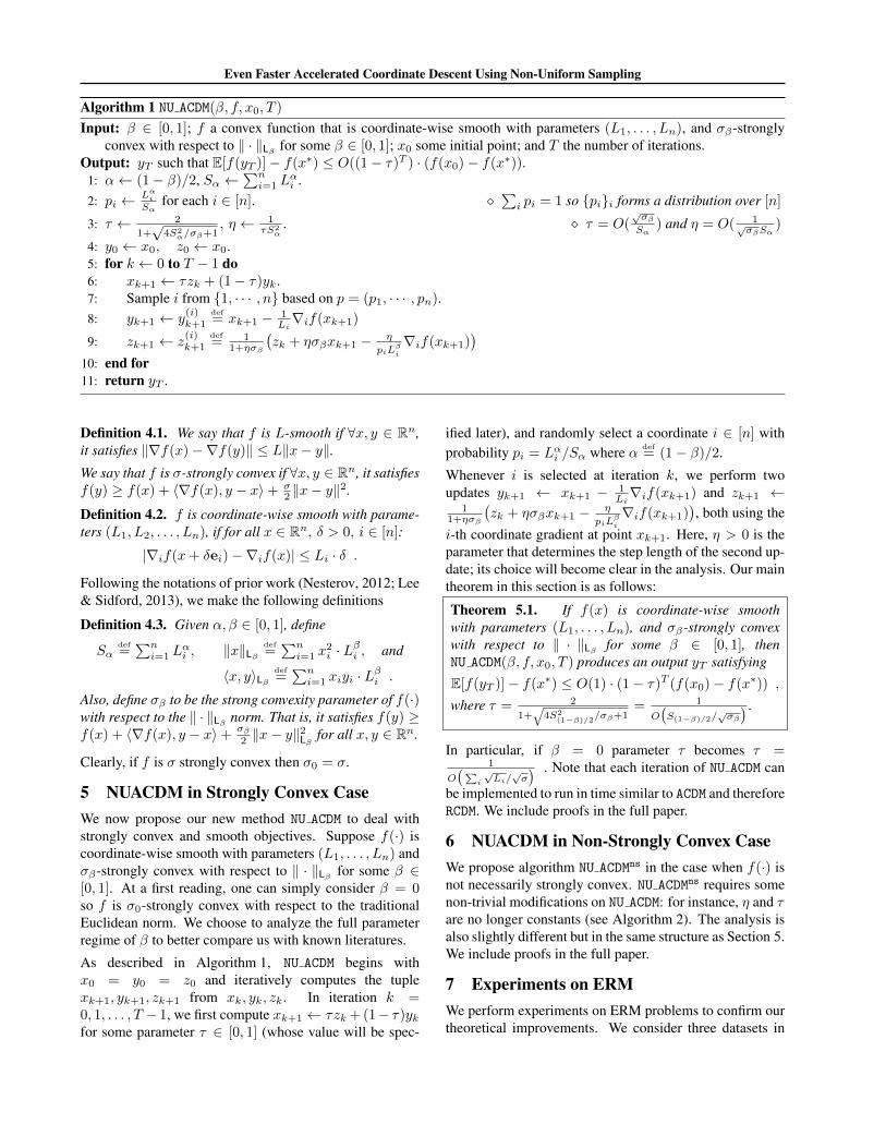
Algorithm 1 NU ACDM(β, f, x0, T )

Input: β ∈ [0, 1]; f a convex function that is coordinate-wise smooth with parameters (L1, . . . , Ln), and σβ-stronglyconvex with respect to ‖ · ‖Lβ for some β ∈ [0, 1]; x0 some initial point; and T the number of iterations.

Output: yT such that E[f(yT )]− f(x∗) ≤ O((1− τ)T ) · (f(x0)− f(x∗)).1: α← (1− β)/2, Sα ←

∑ni=1 L

αi .

2: pi ← LαiSα

for each i ∈ [n]. ∑i pi = 1 so pii forms a distribution over [n]

3: τ ← 2

1+√

4S2α/σβ+1

, η ← 1τS2

α. τ = O(

√σβSα

) and η = O( 1√σβSα

)

4: y0 ← x0, z0 ← x0.5: for k ← 0 to T − 1 do6: xk+1 ← τzk + (1− τ)yk.7: Sample i from 1, · · · , n based on p = (p1, · · · , pn).8: yk+1 ← y

(i)k+1

def= xk+1 − 1

Li∇if(xk+1)

9: zk+1 ← z(i)k+1

def= 1

1+ησβ

(zk + ησβxk+1 − η

piLβi

∇if(xk+1))

10: end for11: return yT .

Definition 4.1. We say that f is L-smooth if ∀x, y ∈ Rn,it satisfies ‖∇f(x)−∇f(y)‖ ≤ L‖x− y‖.We say that f is σ-strongly convex if ∀x, y ∈ Rn, it satisfiesf(y) ≥ f(x) + 〈∇f(x), y − x〉+ σ

2 ‖x− y‖2.

Definition 4.2. f is coordinate-wise smooth with parame-ters (L1, L2, . . . , Ln), if for all x ∈ Rn, δ > 0, i ∈ [n]:

|∇if(x+ δei)−∇if(x)| ≤ Li · δ .

Following the notations of prior work (Nesterov, 2012; Lee& Sidford, 2013), we make the following definitions

Definition 4.3. Given α, β ∈ [0, 1], define

Sαdef=∑ni=1 L

αi , ‖x‖Lβ

def=∑ni=1 x

2i · L

βi , and

〈x, y〉Lβdef=∑ni=1 xiyi · L

βi .

Also, define σβ to be the strong convexity parameter of f(·)with respect to the ‖ · ‖Lβ norm. That is, it satisfies f(y) ≥f(x) + 〈∇f(x), y − x〉+

σβ2 ‖x− y‖

2Lβ

for all x, y ∈ Rn.

Clearly, if f is σ strongly convex then σ0 = σ.

5 NUACDM in Strongly Convex CaseWe now propose our new method NU ACDM to deal withstrongly convex and smooth objectives. Suppose f(·) iscoordinate-wise smooth with parameters (L1, . . . , Ln) andσβ-strongly convex with respect to ‖ · ‖Lβ for some β ∈[0, 1]. At a first reading, one can simply consider β = 0so f is σ0-strongly convex with respect to the traditionalEuclidean norm. We choose to analyze the full parameterregime of β to better compare us with known literatures.

As described in Algorithm 1, NU ACDM begins withx0 = y0 = z0 and iteratively computes the tuplexk+1, yk+1, zk+1 from xk, yk, zk. In iteration k =0, 1, . . . , T − 1, we first compute xk+1 ← τzk + (1− τ)ykfor some parameter τ ∈ [0, 1] (whose value will be spec-

ified later), and randomly select a coordinate i ∈ [n] withprobability pi = Lαi /Sα where α def

= (1− β)/2.

Whenever i is selected at iteration k, we perform twoupdates yk+1 ← xk+1 − 1

Li∇if(xk+1) and zk+1 ←

11+ησβ

(zk + ησβxk+1 − η

piLβi

∇if(xk+1)), both using the

i-th coordinate gradient at point xk+1. Here, η > 0 is theparameter that determines the step length of the second up-date; its choice will become clear in the analysis. Our maintheorem in this section is as follows:

Theorem 5.1. If f(x) is coordinate-wise smoothwith parameters (L1, . . . , Ln), and σβ-strongly convexwith respect to ‖ · ‖Lβ for some β ∈ [0, 1], thenNU ACDM(β, f, x0, T ) produces an output yT satisfying

E[f(yT )]− f(x∗) ≤ O(1) · (1− τ)T (f(x0)− f(x∗)) ,

where τ = 2

1+√

4S2(1−β)/2/σβ+1

= 1

O(S(1−β)/2/

√σβ

) .

In particular, if β = 0 parameter τ becomes τ =1

O(∑

i

√Li/√σ) . Note that each iteration of NU ACDM can

be implemented to run in time similar to ACDM and thereforeRCDM. We include proofs in the full paper.

6 NUACDM in Non-Strongly Convex CaseWe propose algorithm NU ACDMns in the case when f(·) isnot necessarily strongly convex. NU ACDMns requires somenon-trivial modifications on NU ACDM: for instance, η and τare no longer constants (see Algorithm 2). The analysis isalso slightly different but in the same structure as Section 5.We include proofs in the full paper.

7 Experiments on ERMWe perform experiments on ERM problems to confirm ourtheoretical improvements. We consider three datasets in


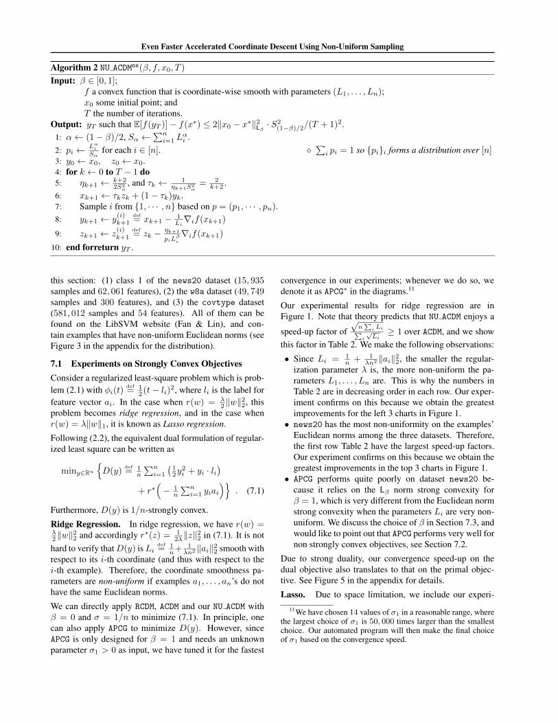
Algorithm 2 NU ACDMns(β, f, x0, T )

Input: β ∈ [0, 1];f a convex function that is coordinate-wise smooth with parameters (L1, . . . , Ln);x0 some initial point; andT the number of iterations.

Output: yT such that E[f(yT )]− f(x∗) ≤ 2‖x0 − x∗‖2Lβ · S2(1−β)/2/(T + 1)2.

1: α← (1− β)/2, Sα ←∑ni=1 L

αi .

2: pi ← LαiSα

for each i ∈ [n]. ∑i pi = 1 so pii forms a distribution over [n]

3: y0 ← x0, z0 ← x0.4: for k ← 0 to T − 1 do5: ηk+1 ← k+2

2S2α

, and τk ← 1ηk+1S2

α= 2

k+2 .6: xk+1 ← τkzk + (1− τk)yk.7: Sample i from 1, · · · , n based on p = (p1, · · · , pn).8: yk+1 ← y

(i)k+1

def= xk+1 − 1

Li∇if(xk+1)

9: zk+1 ← z(i)k+1

def= zk − ηk+1

piLβi

∇if(xk+1)

10: end forreturn yT .

this section: (1) class 1 of the news20 dataset (15, 935samples and 62, 061 features), (2) the w8a dataset (49, 749samples and 300 features), and (3) the covtype dataset(581, 012 samples and 54 features). All of them can befound on the LibSVM website (Fan & Lin), and con-tain examples that have non-uniform Euclidean norms (seeFigure 3 in the appendix for the distribution).

7.1 Experiments on Strongly Convex ObjectivesConsider a regularized least-square problem which is prob-lem (2.1) with φi(t)

def= 1

2 (t− li)2, where li is the label forfeature vector ai. In the case when r(w) = λ

2 ‖w‖22, this

problem becomes ridge regression, and in the case whenr(w) = λ‖w‖1, it is known as Lasso regression.

Following (2.2), the equivalent dual formulation of regular-ized least square can be written as

miny∈RnD(y)

def= 1

n

∑ni=1

(12y

2i + yi · li

)+ r∗

(− 1

n

∑ni=1 yiai

). (7.1)

Furthermore, D(y) is 1/n-strongly convex.

Ridge Regression. In ridge regression, we have r(w) =λ2 ‖w‖

22 and accordingly r∗(z) = 1

2λ‖z‖22 in (7.1). It is not

hard to verify thatD(y) isLidef= 1

n+ 1λn2 ‖ai‖22 smooth with

respect to its i-th coordinate (and thus with respect to thei-th example). Therefore, the coordinate smoothness pa-rameters are non-uniform if examples a1, . . . , an’s do nothave the same Euclidean norms.

We can directly apply RCDM, ACDM and our NU ACDM withβ = 0 and σ = 1/n to minimize (7.1). In principle, onecan also apply APCG to minimize D(y). However, sinceAPCG is only designed for β = 1 and needs an unknownparameter σ1 > 0 as input, we have tuned it for the fastest

convergence in our experiments; whenever we do so, wedenote it as APCG∗ in the diagrams.11

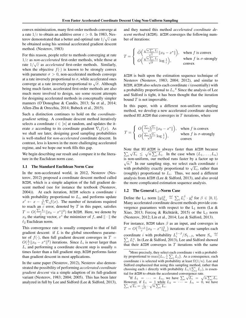
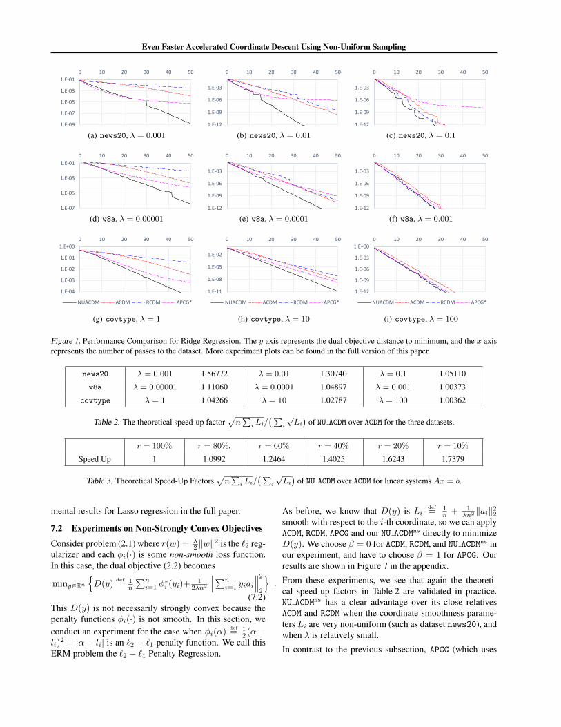
Our experimental results for ridge regression are inFigure 1. Note that theory predicts that NU ACDM enjoys a

speed-up factor of√n∑i Li∑

i

√Li≥ 1 over ACDM, and we show

this factor in Table 2. We make the following observations:

• Since Li = 1n + 1

λn2 ‖ai‖22, the smaller the regular-ization parameter λ is, the more non-uniform the pa-rameters L1, . . . , Ln are. This is why the numbers inTable 2 are in decreasing order in each row. Our exper-iment confirms on this because we obtain the greatestimprovements for the left 3 charts in Figure 1.

• news20 has the most non-uniformity on the examples’Euclidean norms among the three datasets. Therefore,the first row Table 2 have the largest speed-up factors.Our experiment confirms on this because we obtain thegreatest improvements in the top 3 charts in Figure 1.

• APCG performs quite poorly on dataset news20 be-cause it relies on the Lβ norm strong convexity forβ = 1, which is very different from the Euclidean normstrong convexity when the parameters Li are very non-uniform. We discuss the choice of β in Section 7.3, andwould like to point out that APCG performs very well fornon strongly convex objectives, see Section 7.2.

Due to strong duality, our convergence speed-up on thedual objective also translates to that on the primal objec-tive. See Figure 5 in the appendix for details.

Lasso. Due to space limitation, we include our experi-

11We have chosen 14 values of σ1 in a reasonable range, wherethe largest choice of σ1 is 50, 000 times larger than the smallestchoice. Our automated program will then make the final choiceof σ1 based on the convergence speed.


1.E-09

1.E-07

1.E-05

1.E-03

1.E-01

0 10 20 30 40 50

NUACDM ACDM RCDM APCG*(a) news20, λ = 0.001

1.E-12

1.E-09

1.E-06

1.E-03

0 10 20 30 40 50

NUACDM ACDM RCDM APCG*(b) news20, λ = 0.01

1.E-12

1.E-09

1.E-06

1.E-03

0 10 20 30 40 50

NUACDM ACDM RCDM APCG*(c) news20, λ = 0.1

1.E-07

1.E-05

1.E-03

1.E-01

0 10 20 30 40 50

NUACDM ACDM RCDM APCG*(d) w8a, λ = 0.00001

1.E-12

1.E-09

1.E-06

1.E-03

0 10 20 30 40 50

NUACDM ACDM RCDM APCG*(e) w8a, λ = 0.0001

1.E-12

1.E-09

1.E-06

1.E-03

0 10 20 30 40 50

NUACDM ACDM RCDM APCG*(f) w8a, λ = 0.001

1.E-04

1.E-03

1.E-02

1.E-01

1.E+00

0 10 20 30 40 50

NUACDM ACDM RCDM APCG*

(g) covtype, λ = 1

1.E-11

1.E-08

1.E-05

1.E-02

0 10 20 30 40 50


(h) covtype, λ = 10

1.E-12

1.E-09

1.E-06

1.E-03

1.E+00

0 10 20 30 40 50


(i) covtype, λ = 100

Figure 1. Performance Comparison for Ridge Regression. The y axis represents the dual objective distance to minimum, and the x axisrepresents the number of passes to the dataset. More experiment plots can be found in the full version of this paper.

news20 λ = 0.001 1.56772 λ = 0.01 1.30740 λ = 0.1 1.05110

w8a λ = 0.00001 1.11060 λ = 0.0001 1.04897 λ = 0.001 1.00373

covtype λ = 1 1.04266 λ = 10 1.02787 λ = 100 1.00362

Table 2. The theoretical speed-up factor√n∑i Li/

(∑i

√Li)

of NU ACDM over ACDM for the three datasets.

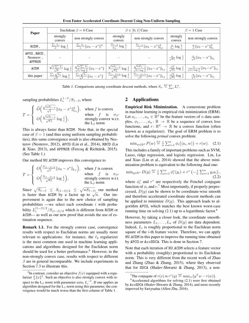
r = 100% r = 80%, r = 60% r = 40% r = 20% r = 10%

Speed Up 1 1.0992 1.2464 1.4025 1.6243 1.7379

Table 3. Theoretical Speed-Up Factors√n∑i Li/

(∑i

√Li)

of NU ACDM over ACDM for linear systems Ax = b.

mental results for Lasso regression in the full paper.

7.2 Experiments on Non-Strongly Convex Objectives

Consider problem (2.1) where r(w) = λ2 ‖w‖

2 is the `2 reg-ularizer and each φi(·) is some non-smooth loss function.In this case, the dual objective (2.2) becomes

miny∈RnD(y)

def= 1

n

∑ni=1 φ

∗i (yi)+

12λn2

∥∥∥∑ni=1 yiai

∥∥∥22

.

(7.2)This D(y) is not necessarily strongly convex because thepenalty functions φi(·) is not smooth. In this section, weconduct an experiment for the case when φi(α)

def= 1

2 (α −li)

2 + |α − li| is an `2 − `1 penalty function. We call thisERM problem the `2 − `1 Penalty Regression.

As before, we know that D(y) is Lidef= 1

n + 1λn2 ‖ai‖22

smooth with respect to the i-th coordinate, so we can applyACDM, RCDM, APCG and our NU ACDMns directly to minimizeD(y). We choose β = 0 for ACDM, RCDM, and NU ACDMns inour experiment, and have to choose β = 1 for APCG. Ourresults are shown in Figure 7 in the appendix.

From these experiments, we see that again the theoreti-cal speed-up factors in Table 2 are validated in practice.NU ACDMns has a clear advantage over its close relativesACDM and RCDM when the coordinate smoothness parame-ters Li are very non-uniform (such as dataset news20), andwhen λ is relatively small.

In contrast to the previous subsection, APCG (which uses


1.E-14

1.E-11

1.E-08

1.E-05

1.E-02

1.E+01

0 50 100 150 200

NUACDM ACDM RandKaczmarz(a) r = 100%

1.E-14

1.E-11

1.E-08

1.E-05

1.E-02

1.E+01

0 50 100 150 200

NUACDM ACDM RandKaczmarz(b) r = 80%

1.E-14

1.E-11

1.E-08

1.E-05

1.E-02

1.E+01

0 50 100 150 200

NUACDM ACDM RandKaczmarz(c) r = 60%

1.E-14

1.E-11

1.E-08

1.E-05

1.E-02

1.E+01

0 50 100 150 200

NUACDM ACDM RandKaczmarz

(d) r = 40%

1.E-14

1.E-11

1.E-08

1.E-05

1.E-02

1.E+01

0 50 100 150 200


(e) r = 20%

1.E-14

1.E-11

1.E-08

1.E-05

1.E-02

1.E+01

0 50 100 150 200


(f) r = 10%

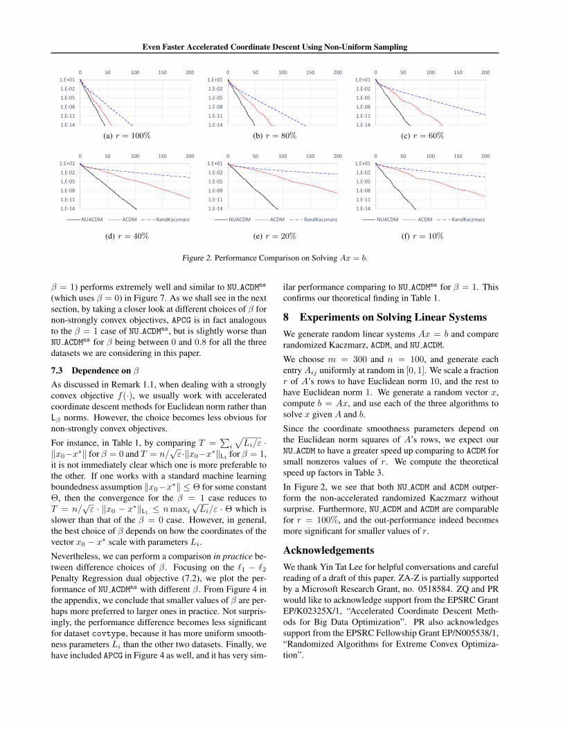
Figure 2. Performance Comparison on Solving Ax = b.

β = 1) performs extremely well and similar to NU ACDMns

(which uses β = 0) in Figure 7. As we shall see in the nextsection, by taking a closer look at different choices of β fornon-strongly convex objectives, APCG is in fact analogousto the β = 1 case of NU ACDMns, but is slightly worse thanNU ACDMns for β being between 0 and 0.8 for all the threedatasets we are considering in this paper.

7.3 Dependence on βAs discussed in Remark 1.1, when dealing with a stronglyconvex objective f(·), we usually work with acceleratedcoordinate descent methods for Euclidean norm rather thanLβ norms. However, the choice becomes less obvious fornon-strongly convex objectives.

For instance, in Table 1, by comparing T =∑i

√Li/ε ·

‖x0−x∗‖ for β = 0 and T = n/√ε·‖x0−x∗‖L1 for β = 1,

it is not immediately clear which one is more preferable tothe other. If one works with a standard machine learningboundedness assumption ‖x0−x∗‖ ≤ Θ for some constantΘ, then the convergence for the β = 1 case reduces toT = n/

√ε · ‖x0 − x∗‖L1 ≤ nmaxi

√Li/ε · Θ which is

slower than that of the β = 0 case. However, in general,the best choice of β depends on how the coordinates of thevector x0 − x∗ scale with parameters Li.

Nevertheless, we can perform a comparison in practice be-tween difference choices of β. Focusing on the `1 − `2Penalty Regression dual objective (7.2), we plot the per-formance of NU ACDMns with different β. From Figure 4 inthe appendix, we conclude that smaller values of β are per-haps more preferred to larger ones in practice. Not surpris-ingly, the performance difference becomes less significantfor dataset covtype, because it has more uniform smooth-ness parameters Li than the other two datasets. Finally, wehave included APCG in Figure 4 as well, and it has very sim-

ilar performance comparing to NU ACDMns for β = 1. Thisconfirms our theoretical finding in Table 1.

8 Experiments on Solving Linear SystemsWe generate random linear systems Ax = b and comparerandomized Kaczmarz, ACDM, and NU ACDM.

We choose m = 300 and n = 100, and generate eachentryAij uniformly at random in [0, 1]. We scale a fractionr of A’s rows to have Euclidean norm 10, and the rest tohave Euclidean norm 1. We generate a random vector x,compute b = Ax, and use each of the three algorithms tosolve x given A and b.

Since the coordinate smoothness parameters depend onthe Euclidean norm squares of A’s rows, we expect ourNU ACDM to have a greater speed up comparing to ACDM forsmall nonzeros values of r. We compute the theoreticalspeed up factors in Table 3.

In Figure 2, we see that both NU ACDM and ACDM outper-form the non-accelerated randomized Kaczmarz withoutsurprise. Furthermore, NU ACDM and ACDM are comparablefor r = 100%, and the out-performance indeed becomesmore significant for smaller values of r.

AcknowledgementsWe thank Yin Tat Lee for helpful conversations and carefulreading of a draft of this paper. ZA-Z is partially supportedby a Microsoft Research Grant, no. 0518584. ZQ and PRwould like to acknowledge support from the EPSRC GrantEP/K02325X/1, “Accelerated Coordinate Descent Meth-ods for Big Data Optimization”. PR also acknowledgessupport from the EPSRC Fellowship Grant EP/N005538/1,“Randomized Algorithms for Extreme Convex Optimiza-tion”.


ReferencesAllen-Zhu, Zeyuan. Katyusha: The First Truly Accel-

erated Stochastic Gradient Method. ArXiv e-prints,abs/1603.05953, March 2016.

Allen-Zhu, Zeyuan and Hazan, Elad. Optimal Black-BoxReductions Between Optimization Objectives. ArXiv e-prints, abs/1603.05642, March 2016.

Allen-Zhu, Zeyuan and Orecchia, Lorenzo. Linear cou-pling: An ultimate unification of gradient and mirror de-scent. ArXiv e-prints, abs/1407.1537, July 2014.

Allen-Zhu, Zeyuan, Yuan, Yang, and Sridharan, Karthik.Exploiting the Structure: Stochastic Gradient MethodsUsing Raw Clusters. ArXiv e-prints, abs/1602.02151,February 2016.

Bubeck, Sebastien, Lee, Yin Tat, and Singh, Mohit. A geo-metric alternative to Nesterov’s accelerated gradient de-scent. ArXiv e-prints, abs/1506.08187, June 2015.

Csiba, Dominik, Qu, Zheng, and Richtarik, Peter. Stochas-tic dual coordinate ascent with adaptive probabilities.In Proceedings of the 32nd International Conference onMachine Learning, ICML 2015, Lille, France, 6-11 July2015, pp. 674–683, 2015.

Fan, Rong-En and Lin, Chih-Jen. LIBSVM Data: Classifi-cation, Regression and Multi-label. Accessed: 2015-06.

Fercoq, Olivier and Richtarik, Peter. Accelerated, paral-lel, and proximal coordinate descent. SIAM Journal onOptimization, 25(4):1997–2023, 2015. First appeared onArXiv 1312.5799 in 2013.

Gower, Robert M. and Richtarik, Peter. Stochastic dual as-cent for solving linear systems. arXiv:1512.06890, 2015.

Kaczmarz, Stefan. Angenaherte auflosung von syste-men linearer gleichungen. Bulletin International de lA-cademie Polonaise des Sciences et des Lettres, 35:355–357, 1937.

Lee, Yin Tat and Sidford, Aaron. Efficient accelerated coor-dinate descent methods and faster algorithms for solvinglinear systems. In Proceedings of the 54th Annual Sym-posium on Foundations of Computer Science (FOCS),pp. 147–156. IEEE, 2013.

Lin, Qihang, Lu, Zhaosong, and Xiao, Lin. An AcceleratedProximal Coordinate Gradient Method and its Applica-tion to Regularized Empirical Risk Minimization. In Ad-vances in Neural Information Processing Systems, NIPS2014, pp. 3059–3067, 2014.

Lu, Zhaosong and Xiao, Lin. On the complexity analysis ofrandomized block-coordinate descent methods. Mathe-matical Programming, pp. 1–28, 2013.

Needell, Deanna, Ward, Rachel, and Srebro, Nati. Stochas-tic gradient descent, weighted sampling, and the ran-domized kaczmarz algorithm. In Advances in Neural In-formation Processing Systems 27, pp. 1017–1025, 2014.

Nesterov, Yurii. A method of solving a convex program-ming problem with convergence rate O(1/k2). In Dok-lady AN SSSR (translated as Soviet Mathematics Dok-lady), volume 269, pp. 543–547, 1983.

Nesterov, Yurii. Introductory Lectures on Convex Program-ming Volume: A Basic course, volume I. Kluwer Aca-demic Publishers, 2004. ISBN 1402075537.

Nesterov, Yurii. Smooth minimization of non-smooth func-tions. Mathematical Programming, 103(1):127–152,December 2005. ISSN 0025-5610.

Nesterov, Yurii. Efficiency of Coordinate Descent Methodson Huge-Scale Optimization Problems. SIAM Journalon Optimization, 22(2):341–362, jan 2012. ISSN 1052-6234.

Nesterov, Yurii and Stich, Sebastian. Efficiency of acceler-ated coordinate descent method on structured optimiza-tion problems. Technical report, CORE Discussion Pa-pers, March 2016.

Nutini, Julie, Schmidt, Mark, Laradji, Issam, Friedlan-der, Michael, and Koepke, Hoyt. Coordinate descentconverges faster with the gauss-southwell rule than ran-dom selection. In Proceedings of the 32nd InternationalConference on Machine Learning (ICML-15), pp. 1632–1641, 2015.

O’Donoghue, Brendan and Candes, Emmanuel. AdaptiveRestart for Accelerated Gradient Schemes. Foundationsof Computational Mathematics, July 2013. ISSN 1615-3375.

Qu, Zheng and Richtarik, Peter. Coordinate descent meth-ods with arbitrary sampling I: Algorithms and complex-ity. arXiv:1412.8060, 2014.

Qu, Zheng, Richtarik, Peter, and Zhang, Tong. Ran-domized dual coordinate ascent with arbitrary sampling.CoRR, abs/1411.5873, 2014.

Shalev-Shwartz, Shai and Zhang, Tong. Stochastic dual co-ordinate ascent methods for regularized loss minimiza-tion. Journal of Machine Learning Research, 14:567–599, 2013.

Shalev-Shwartz, Shai and Zhang, Tong. Accelerated Prox-imal Stochastic Dual Coordinate Ascent for RegularizedLoss Minimization. In Proceedings of the 31st Inter-national Conference on Machine Learning, ICML 2014,pp. 64–72, 2014.


Strohmer, Thomas and Vershynin, Roman. A random-ized kaczmarz algorithm with exponential convergence.Journal of Fourier Analysis and Applications, 15(2):262–278, 2009.

Su, Weijie, Boyd, Stephen, and Candes, Emmanuel. Adifferential equation for modeling nesterovs acceleratedgradient method: Theory and insights. In Advances inNeural Information Processing Systems, pp. 2510–2518,2014.

Zhang, Yuchen and Xiao, Lin. Stochastic Primal-Dual Co-ordinate Method for Regularized Empirical Risk Mini-mization. In Proceedings of the 32nd International Con-ference on Machine Learning, ICML 2015, 2015.

Zhao, Peilin and Zhang, Tong. Stochastic Optimizationwith Importance Sampling for Regularized Loss Mini-mization. In Proceedings of the 32nd International Con-ference on Machine Learning, volume 37, pp. 1–9, 2015.

Documents

Even Faster Accelerated Coordinate Descent Using …proceedings.mlr.press/v48/allen-zhuc16.pdf · Even Faster Accelerated Coordinate Descent Using Non-Uniform Sampling Paper Euclidean