EVOLUTION OF THE HOUSEHOLD VEHICLE FLEET:

ANTICIPATING FLEET COMPOSITION, PHEV ADOPTION AND GHG

EMISSIONS IN AUSTIN, TEXAS

Sashank Musti

Graduate Research Assistant

The University of Texas at Austin – 6.508, E. Cockrell Jr. Hall

Austin, TX 78712-1076 sashankmnm@gmail.com

Kara M. Kockelman

(Corresponding author)

Professor and William J. Murray Jr. Fellow

Department of Civil, Architectural and Environmental Engineering

The University of Texas at Austin – 6.9 E. Cockrell Jr. Hall Austin,

TX 78712-1076

kkockelm@mail.utexas.edu

Phone: 512-471-0210 & FAX: 512-475-8744

The following paper is a pre-print and the final publication can be found in

Transportation Research Part A, 45 (8):707-720, 2011.

Key Words: Vehicle choice, fleet evolution, vehicle ownership, plug-in hybrid electric vehicles

(PHEVs), climate change policy, stated preference, opinion survey, microsimulation ABSTRACT

In today‟s world of volatile fuel prices and climate concerns, there is little study on the relation

between vehicle ownership patterns and attitudes toward potential policies and vehicle

technologies. This work provides new data on ownership decisions and owner preferences under

various scenarios, coupled with calibrated models to microsimulate Austin‟s personal-fleet

evolution. Results suggest that most Austinites (63%, population-corrected share) support a

feebate policy to favor more fuel efficient vehicles. Top purchase criteria are price, type/class,

and fuel economy (with 30%, 21% and 19% of respondents placing these in their top three).

Most (56%) respondents also indicated that they would consider purchasing a PHEV if it were to

cost $6,000 more than its conventional, gasoline-powered counterpart. And many respond

strongly to signals on the external (health and climate) costs of a vehicle‟s emissions, more

strongly than they respond to information on fuel cost savings.

25-year forecasts suggest that 19% of Austin‟s vehicle fleet could be comprised of HEVs and

PHEVs under adoption of a feebate policy along with PHEV availability in Year 1 of the

simulation. Vehicle usage levels are predicted to increase overall, along with average vehicle

ownership levels (per household, and per capita); and a feebate policy is predicted to raise total

VMT slightly (just 3 percent, by simulation year 25, relative to the trend scenario) while

reducing CO2 emissions only slightly (by 5.13 percent, relative to trend).Two- and three-vehicle

households are observed to be the highest (simulated) adopters of HEVs and PHEVs across all

scenarios. And HEVs, PHEVs and Smart Cars are estimated to represent a major share of the

fleet‟s VMT (25%) by year 25 under the feebate scenario. The combined share of vans, pickup

trucks, SUVs, and CUVs is lowest under the feebate scenario, at 35% (versus 47% in Austin‟s

current household fleet and 44% under the TREND scenario), yet feebate-policy receipts exceed

rebates in each simulation year. With the highest share of PHEVs (6.14%) across all the

scenarios, CO2 emissions are down by 3.14% under the LOWPRICE scenario. In the longer

term, tax incentives, feebates and purchase prices along with government-industry partnerships,

accurate information on range, recharging times to increase customer confidence should have

even more significant effects on energy dependence and greenhouse gas emissions.

INTRODUCTION AND MOTIVATION

Climate change is one of the planet‟s top issues. The U.S. contains 4% of the world's population

but produces 25% of all greenhouse gas (GHG) emissions (BBC, 2002), with 28% of these

emanating from the transportation sector alone (EIA, 2006). Rising gasoline prices, emerging

engine technologies, and changes in fuel-economy policies are anticipated to result in a variety

of behavioral changes. These changes include adjustments in vehicle occupancies, trip

destinations, trip chaining, and mode choice in the short term. In the longer term, a wider sphere

of decisions will be affected, including household vehicle holdings (number, make and model),

vehicle purchase and retirement timing, and home and work location choices.

Automobile ownership plays an extremely important role in determining vehicle use, vehicle

emissions, fuel consumption, highway capacity, congestion, and traffic safety. A relatively new

yet key objective of transportation planners and researchers is to know how many and what type

of automobiles are owned by households, how they adjust their fleet, and how many miles they

drive each of their vehicles. The benefits that a household derives from its fleet depend on use

levels, type of vehicles owned, household demographics and other factors. To accurately

anticipate future fleet attributes (and therefore emissions, gas tax receipts, crash counts, and so

forth), planners must have dependable forecasts of vehicle ownership and use.

This study examines opinions on vehicle policy and models the evolution of the household fleet

via transaction and choice decisions over a 25-year period (from 2009 to 2034). A

microsimulation framework based on a set of interwoven models for vehicle ownership and use

yields future vehicle composition mix along with GHG emissions forecasts in Austin, Texas. The

following sections discuss recent literature on vehicle choice, questionnaire design and data

acquisition, sample correction, geo-coding and sample data characteristics. The paper then

presents results of data analysis, including vehicle choice, vehicle retirement and transactions

timing; and the results of a 25-year simulation results. The paper concludes with a summary of

results, recommendations, conclusions and ideas for topic extension.

EXISTING STUDIES

Much existing research on vehicle type choice is based on vehicle attributes, household

characteristics, and fuel costs. Manski and Sherman (1976) developed separate multinomial logit

models for the number of vehicles owned and vehicle type for households owing one or two

vehicles. Lave and Train (1979) controlled for several household attributes, vehicle

characteristics, gasoline prices, and taxes on larger vehicles and found that higher income

households tend to prefer expensive cars and younger individuals prefer high-performance cars.

Berkovec (1985) developed nested logit models, with the upper-level for number of vehicles and

the lower-level nest for vehicle class with vehicle attributes serving as exogenous variables. This

disaggregate model of vehicle choice was used to forecast U.S. automobile sales, vehicle

retirements and fleet attributes for the 1984-1990 period. Results from such studies illuminate the

relative importance of capital costs, operating costs, cargo space, and performance on vehicle

choice with findings similar to those in Berkovec and Rust (1985), Mohammadian and Miller

(2003) and Mannering et al. (2002).

Consumers‟ travel habits and behavioral attitudes also affect vehicle choice. Choo and

Mokatarian (2004) found that travel attitudes, personality, lifestyle, and mobility factors are

useful in forecasting vehicle types owned and predicting the most-used vehicle within a

household. Kurani and Turrentine (2004) found that purchasing households do not pay much

attention to fuel costs over time, unless they are under severe economic constraints. A vehicle‟s

overall visual appeal, amenities, reliability and safety, cabin size, acceleration, purchase price

and other amenities are found to have a more significant effect on choice. Gallagher and

Muehlegger (2008) studied consumer adoption of hybrid electric vehicles (HEVs) in the U.S.

and found that groups with strong preferences for environmentalism and energy security prefer

HEV. Their results show that rising gasoline prices and social preferences result in cause

maximum sales.

Consumer‟s previous vehicle experiences and brand loyalty can also affect choice and use.

Extending Dubin and McFadden‟s (1984) work, Mannering and Winston (1985) employed a

dynamic utilization framework for vehicle choice (and use) as a function of the prior year‟s

utilization (a brand loyalty measure), household characteristics, and vehicle attributes. Roy‟s

Identity (Roy, 1947) was used to link an indirect utility function for vehicle choice with vehicle

use (annual VMT). A multinomial logit model conditioned on vehicle choice was employed to

anticipate the number of vehicles owned. Employing similar models, Feng et al. (2005) studied

the effect of gas taxes and subsidies on VMT, vehicle choice, and emissions. As expected, their

results suggest VMT reductions, a shift away from sport-utility vehicles (SUVs), and greater use

of a household‟s smaller cars under a scenario of higher fuel costs.

The impact of land use variables is also of interest. Train (1980) examined vehicle ownership

and work trip mode choices and concluded that households living near their work places or

having more access to transit will reduce the number of vehicles owned. Zhao and Kockelman

(2000) developed a multivariate negative binomial model to predict vehicle ownership by vehicle

type. Their results suggest that ownership decisions are firmly related to household size, income,

population density (in zone of residence), and vehicle prices. Fang (2008) developed a Bayesian

multivariate ordinal response system to model vehicle choice and usage and found higher

residential densities to be associated with lower vehicle utilization and fewer light-duty truck

holdings, consistent with Zhao and Kockelman‟s (2000) findings. Bhat and Sen (2006) and Bhat

et al. (2008) also conclude that vehicle-holdings and miles of travel vary with demographic

characteristics, vehicle attributes, fuel costs, other travel costs and nei ghborhood characteristics.

Finally, life course events also affect vehicle holdings. Mohammadian and Miller (2003b)

developed a dynamic transactions model using retrospective panel data collected in Toronto.

Their results suggest that recent changes in the number of household workers, adults, driving

licenses, and household size will prompt acquisition of a new car or replace a vehicle. Prillwitz et

al. (2006) found positive correlation between vehicle transactions and a change in the number of

adults, birth of the first child, change in monthly income, and change in residence.

This research builds on the extensive existing literature, by examining PHEV and minicar (Smart

Car) adoption and household attitudes toward vehicle design and energy policies, with forward-

year fleet-simulation under higher gas prices and feebate policies.

DATA DESCRIPTION

Microsimulation models seek to replicate the evolution of individual agents like households, for

predictive purposes. Here they are used to anticipate the vehicle ownership, use and associated

GHG emissions of households over a 25- year horizon in the Austin, Texas region. Such models

are generally data intensive, and this section briefly describes the various data sets analyzed.

Household Data Sets

Sub-models for simulating the household and individual evolution process were taken from

various studies. Model results and their accompanying data sets from Tirumalachetty et al.

(2009), Tirumalachetty and Kockelman (2010), and Bina and Kockelman (2006) were used in

the framework.

Vehicle Ownership and Transactions Data

This subsection describes the data acquisition efforts for estimating the vehicle acquisition, use

and transaction models. General observations on consumers‟ vehicle preferences and their

opinions of relevant policies are also provided.

The data comes from a web-based springtime-2009 survey of Austin-area households. The

survey was designed to understand household fleet evolution along with public opinion. Data

were collected on current, past vehicle holdings and use, intended future holdings, type of

acquisition (for example. leased versus purchased new or used), and reasons behind vehicle

acquisition and loss/retirement.

Respondents selected one of 12 new vehicles they would most likely acquire under four different

scenarios. The options were randomized across scenarios and across respondents. Images for

each vehicle, purchase prices and informative links on each vehicle (via www.edmunds.com)

were provided. The first scenario‟s, 12 alternatives were also accompanied by fuel economy and

average yearly fuel expenses (assuming 15,000 miles of travel with fuel at $2.50 per gallon). The

12 vehicles covered a wide spectrum of vehicles, from very low to very high fuel economy, and

low to very high purchase price. The vehicles encompassed all major body types: small,

compact, mid-sized, large, and luxury cars; a minivan; a pickup truck; two cross-over1/sport

utility vehicles; a Prius hybrid electric vehicle (HEV); a Prius plug-in HEV (PHEV); and a

Hummer. Information from Kurani et al. (2009), Axsen and Kurani (2008), Markel (2006a),

1 CUVs are vehicles that borrow features from SUVs but have a car platform for lighter weight and better fuel

efficiency.

Markel (2006b), and CalCars.com was used to estimate the PHEV‟s effective fuel economy and

purchase price. Assumptions include a 30-mile all-electric range (PHEV30) requiring about 250

watt-hours per mile, with an 11-gallon gas tank, resulting in a total range over 500 miles. All

other attributes of the PHEV30 matched a Toyota Prius2.

Scenarios two and three had gas prices at $5 and $7 per gallon. In the final (fourth) scenario,

estimates of the monetary value of the global warming and health costs of each vehicle, from

driving 15,000 miles each year, were presented for each of the 12 vehicles. These external costs

for most vehicles were taken from Lemp and Kockelman (2008), but estimates had to be created

for the PHEV option, using Small and Kazimi‟s (1995) morbidity and mortality costs by

pollutant type and the U.S. EIA‟s estimates of pollution from electricity generation (EIA, 2002).

Concerns about PHEV battery disposal were also taken into consideration during this

calculation. First Electric Coop (2009) and CalCars.com indicate that the new lithium battery

disposal should not pose an environmental issue. Thus, the climate and health cost of driving a

PHEV30 15,000 miles a year was expected to range from just $65 to $95 (depending on whether

users drive 41miles per day 7 days per week or 50 miles per day 5 days per week). In contrast,

the Mercedes Smart Car was estimated to impose an annual external cost of $3003 and the

Hummer $965 per year.

The next set of questions sought respondents‟ attitudes toward various policies and engine

technologies that encourage higher fuel economies. The final section of the survey sought

demographic information (including age, household size, income, worker, student status and

home location).

Survey Distribution

To achieve lower cost with wide distribution in the Austin area, the survey was web-based.

Relative to other options, web-based surveys facilitate design flexibility while speeding data

assembly and reducing acquisition costs, and they have the potential to better represent one‟s

target population (Smith et al. 2009a)4. Neighborhood associations and 160 community

organizations (from the regional transit agency and the University of Texas to the lesser-known

Austin Pug Club society) were contacted to broadcast the survey link through their networks. In

addition, 650 respondents to an earlier energy survey (Musti et al., 2009) were contacted.

Results and Summary Statistics

Weights were developed by first dividing the sample into 720 categories, based on gender, age,

worker and student status, household size and household income categories. Categories with too

few data points were merged, and ratios of Austin‟s Public Use Microdata Sample (PUMS)

counts to respondent counts were then normalized, resulting in 645 usable records for data

2 The Chevrolet Volt (BEV) should be launched in 2010 (according to www.chevrolet.com). Prius PHEVs are

expected by 2011 (Sperling and Lutsey, 2009), but some Prius HEV owners have modified their vehicles to charge

from home now (Kurani et al., 2009). 3 The high externality cost for the Smart Car is due to the electric power range requiring about 35.5 watt-hours per

mile (www.fueleconomy.gov). 4 Smith et al. (2009a) collected travel data using multiple recruitment methods at once, in various U.S. locations, and

found that those responding via the Internet did not differ from the general population in any significant way. In fact,

in certain dimensions Internet respondents can be more representative than those electing other response methods.

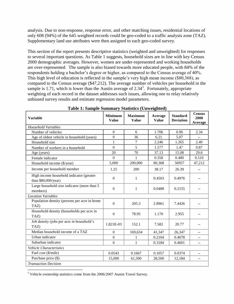
analysis. Due to non-response, response error, and other matching issues, residential locations of

only 608 (94%) of the 645 weighted records could be geo-coded to a traffic analysis zone (TAZ).

Supplementary land use attributes were then assigned to each geo-coded survey.

This section of the report presents descriptive statistics (weighted and unweighted) for responses

to several important questions. As Table 1 suggests, household sizes are in line with key Census

2000 demographic averages. However, women are under-represented and working households

are over-represented. The sample is also biased towards more educated people, with 84% of the

respondents holding a bachelor‟s degree or higher, as compared to the Census average of 40%.

This high level of education is reflected in the sample‟s very high mean income ($80,368), as

compared to the Census average ($47,212). The average number of vehicles per household in the

sample is 1.71, which is lower than the Austin average of 2.345. Fortunately, appropriate

weighting of each record in the dataset addresses such issues, allowing one to relay relatively

unbiased survey results and estimate regression model parameters.

Table 1: Sample Summary Statistics (Unweighted)

Variable Minimum

Value

Maximum

Value

Average

Value

Standard

Deviation

Census

2000

Average

Household Variables

Number of vehicles 0 6 1.706 0.96 2.34

Age of oldest vehicle in household (years) 0 36 6.21 5.07 --

Household size 1 7 2.246 1.265 2.40

Number of workers in a household 0 5 1.577 1.47 0.87

Age (years) 20 70 37.13 15.08 29.6

Female indicator 0 1 0.358 0.480 0.510

Household income ($/year) 5,000 200,000 80,368 56957 47,212

Income per household member 1.25 200 38.17 26.39 --

High income household indicator (greater

than $80,000/year) 0 1 0.4503 0.4976 --

Large household size indicator (more than 5

members) 0 1 0.0488 0.2155 --

Location Variables

Population density (persons per acre in home

TAZ) 0 205.3 2.8961 7.4426 --

Household density (households per acre in

TAZ) 0 78.95 1.170 2.955 --

Job density (jobs per acre in household‟s

TAZ) 1.821E-03 152.1 7.582 20.77 --

Median household income of a TAZ 0 169,634 41,347 26,347 --

Urban indicator 0 1 0.2104 0.4078 --

Suburban indicator 0 1 0.3184 0.4601 --

Vehicle Characteristics

Fuel cost ($/mile) 0.0543 0.1667 0.1057 0.0374 --

Purchase price ($) 15,000 61,500 28,500 12,184 --

Transaction Decision

5 Vehicle ownership statistics come from the 2006/2007 Austin Travel Survey.

Acquire 0 1 0.2214 0.4155 --

Dispose 0 1 0.0511 0.2203 --

Do nothing (neither acquire nor dispose) 0 1 0.7276 0.4456 --

Note: Zones were coded by CAMPO based on a TxDOT formula using a combination of employment and

household density values, with thresholds of 8, 3 and 1 person-equivalents per acre for urban, suburban and rural

area respectively.

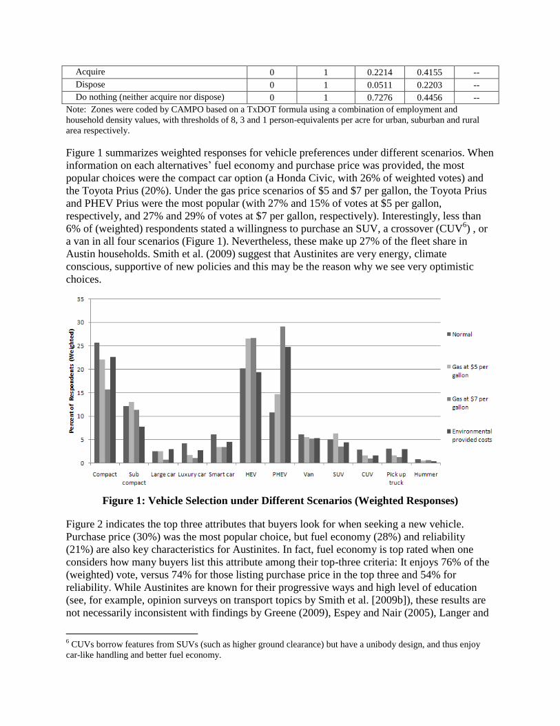
Figure 1 summarizes weighted responses for vehicle preferences under different scenarios. When

information on each alternatives‟ fuel economy and purchase price was provided, the most

popular choices were the compact car option (a Honda Civic, with 26% of weighted votes) and

the Toyota Prius (20%). Under the gas price scenarios of $5 and $7 per gallon, the Toyota Prius

and PHEV Prius were the most popular (with 27% and 15% of votes at $5 per gallon,

respectively, and 27% and 29% of votes at $7 per gallon, respectively). Interestingly, less than

6% of (weighted) respondents stated a willingness to purchase an SUV, a crossover (CUV6) , or

a van in all four scenarios (Figure 1). Nevertheless, these make up 27% of the fleet share in

Austin households. Smith et al. (2009) suggest that Austinites are very energy, climate

conscious, supportive of new policies and this may be the reason why we see very optimistic

choices.

Figure 1: Vehicle Selection under Different Scenarios (Weighted Responses)

Figure 2 indicates the top three attributes that buyers look for when seeking a new vehicle.

Purchase price (30%) was the most popular choice, but fuel economy (28%) and reliability

(21%) are also key characteristics for Austinites. In fact, fuel economy is top rated when one

considers how many buyers list this attribute among their top-three criteria: It enjoys 76% of the

(weighted) vote, versus 74% for those listing purchase price in the top three and 54% for

reliability. While Austinites are known for their progressive ways and high level of education

(see, for example, opinion surveys on transport topics by Smith et al. [2009b]), these results are

not necessarily inconsistent with findings by Greene (2009), Espey and Nair (2005), Langer and

6 CUVs borrow features from SUVs (such as higher ground clearance) but have a unibody design, and thus enjoy

car-like handling and better fuel economy.

Miller (2008) and Turrentine and Kurani (2004). Their pointed examinations of vehicle choice

vis-à-vis fuel economy caused them to conclude that households neglect much future gasoline-

related savings when evaluating the effective purchase price of a vehicle (unless severe

economic constraints exist). In fact, as shown later, a logit model for vehicle preferences does

not enjoy a statistically significant coefficient on fuel economy, though it is somewhat practically

significant (and can be quite core to behavioral response in the simulation), so some neglect of

fuel costs in final choice is apparent, even in this sample. In fact, the model‟s parameter

estimates suggest an effective discount rate of well over 30% per year (in order to equate $1 in

the present valuation of likely gas savings to $1 in purchase price). 30% applies only at an

unusually low 5,000 miles-travelled-per-year assumption. At 10,000 miles per year, the implicit

discount rate is a whopping 102%. (In other words, stated preference results suggest that these

Austin respondents value only a year or two of fuel-cost savings.)

Figure 2: Top Three Attributes for Vehicle Selection (Weighted Responses)

Another interesting feature of the simple responses, as given directly in the data set, is support

for proposed policies. The majority of respondents (63%, population-weighted) indicated support

for a feebate policy (on the sale of vehicles), with vehicles over 30 mi/gal fuel economy enjoying

a rebate, and those under 30 mi/gal paying a premium. (The survey form indicated, for example,

a $3,000 rebate on 40+ mi/gal vehicles, versus a $1,000 fee for 25 mi/gal vehicles and a $4,000

fee for those averaging 10 mi/gal or less.) 56% of respondents indicated that they are ready to

purchase a PHEV, even if it costs $6,000 more than its conventionally fueled counterpart.

Related to this, 55% of the weighted respondents reported that they have access to electricity in

their garage or a carport near their residential unit. This is very consistent with Axsen and

Kurani‟s (2008) recent survey result, that 52% of new vehicle buyers in the U.S. have convenient

access to a home outlet for PHEV recharging.

MODEL RESULTS

While straightforward weighted averages of survey results are one way to exploit the data,

multivariate relationships exist, and these inform models of who is likely to do what and when.

Here, a microsimulation of vehicle holdings is based on a set of interwoven models with annual

transitions. The first stage is annual application of a vehicle transactions model that simulates the

decision to acquire, dispose of or keep a vehicle (in each year). Monte Carlo methods are then

used to ascertain the choice of each household without weighting. In the case of a “buy”

decision, the stated preference vehicle choice probabilities of purchase by vehicle class

determine the type of vehicle class acquired by the household (again using Monte Carlos

methods). In the case of a “sell” decision, vehicles with the lowest systematic utility7 (within a

selling household) were identified and removed. In the “do nothing” case, all vehicles were

retained. A variety of scenarios were simulated, as discussed below, after presentation of model

estimation results. The (current-) vehicle ownership model was not used for vehicle acquisitions,

because the current fleet includes rather few PHEVs or many Smart Cars and HEVs (since these

have not been around long, if at all). Nevertheless, it provides meaningful results of revealed

behavior and serves as a useful counterpart to the stated preference model results, discussed

below. And this current-vehicle ownership model was used in the vehicle disposal stage, where

the lowest utility vehicle is disposed of.

Several different model specifications were explored, including a variety of interaction effects

(across covariates). The final specifications were obtained based on a systematic process of

eliminating variables that did not show statistical significance (at the 95% confidence level). Yet

variables enjoying meaningful practical significance were kept in the model specification, even if

they had t-statistics near 1.0 (or p-values up to 0.34). For example, employment and population

densities were regularly removed, due to very low t-statistics, while indicators for rural, suburban

and urban areas (which are based on job-equivalent densities) were often retained, with t-

statistics around 1.2. These results are presented here now.

Vehicle Ownership Model Results

While this first model specification, for patterns of current vehicle holdings, does not indicate

current purchase preferences, it provides meaningful results of revealed behavior and serves as a

useful counterpart to the stated preference model results, discussed below. Table 2 presents the

results from the multinomial logit model for vehicle class for the data set‟s 596 (geocoded)

vehicle-holding households.

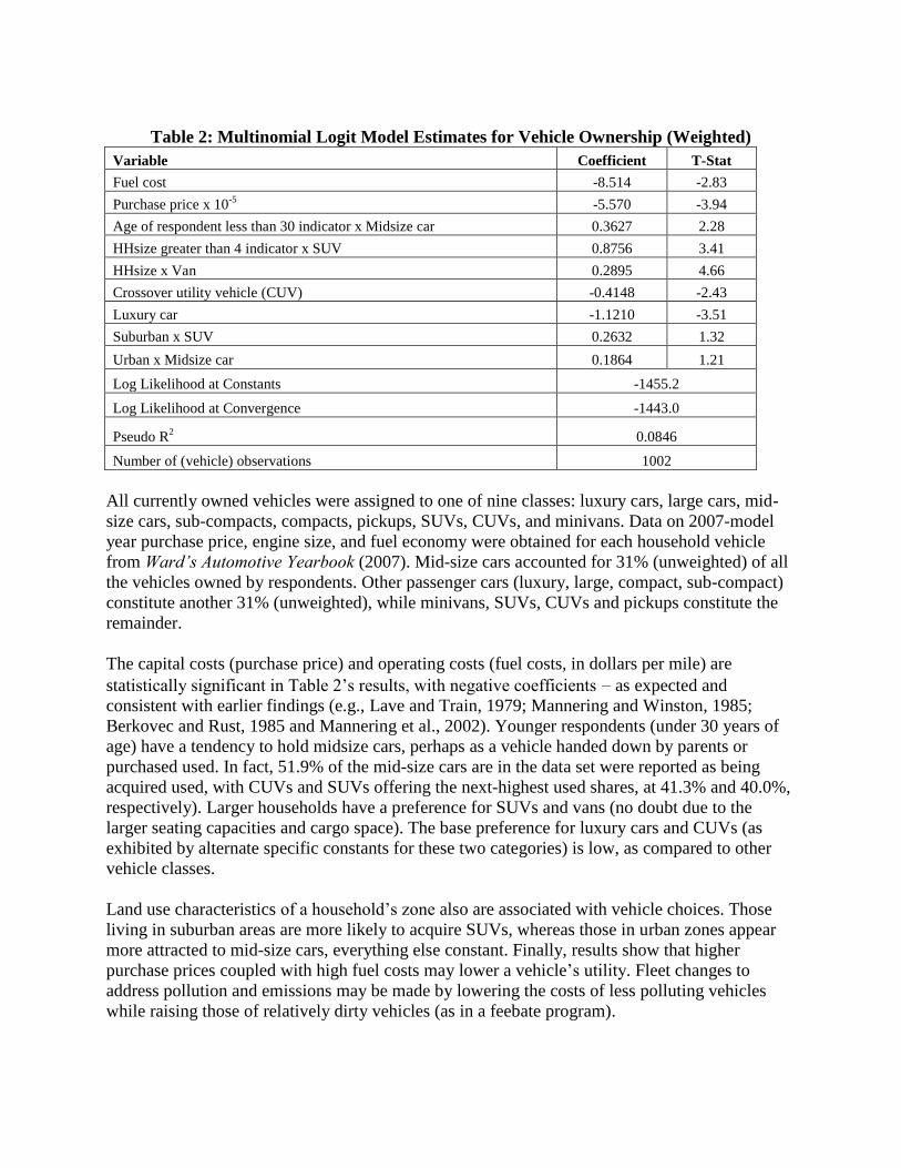
Table 2: Multinomial Logit Model Estimates for Vehicle Ownership (Weighted)

Variable Coefficient T-Stat

Fuel cost -8.514 -2.83

Purchase price x 10-5

-5.570 -3.94

Age of respondent less than 30 indicator x Midsize car 0.3627 2.28

HHsize greater than 4 indicator x SUV 0.8756 3.41

HHsize x Van 0.2895 4.66

Crossover utility vehicle (CUV) -0.4148 -2.43

Luxury car -1.1210 -3.51

Suburban x SUV 0.2632 1.32

Urban x Midsize car 0.1864 1.21

Log Likelihood at Constants -1455.2

Log Likelihood at Convergence -1443.0

Pseudo R2 0.0846

Number of (vehicle) observations 1002

All currently owned vehicles were assigned to one of nine classes: luxury cars, large cars, mid-

size cars, sub-compacts, compacts, pickups, SUVs, CUVs, and minivans. Data on 2007-model

year purchase price, engine size, and fuel economy were obtained for each household vehicle

from Ward’s Automotive Yearbook (2007). Mid-size cars accounted for 31% (unweighted) of all

the vehicles owned by respondents. Other passenger cars (luxury, large, compact, sub-compact)

constitute another 31% (unweighted), while minivans, SUVs, CUVs and pickups constitute the

remainder.

The capital costs (purchase price) and operating costs (fuel costs, in dollars per mile) are

statistically significant in Table 2‟s results, with negative coefficients as expected and

consistent with earlier findings (e.g., Lave and Train, 1979; Mannering and Winston, 1985;

Berkovec and Rust, 1985 and Mannering et al., 2002). Younger respondents (under 30 years of

age) have a tendency to hold midsize cars, perhaps as a vehicle handed down by parents or

purchased used. In fact, 51.9% of the mid-size cars are in the data set were reported as being

acquired used, with CUVs and SUVs offering the next-highest used shares, at 41.3% and 40.0%,

respectively). Larger households have a preference for SUVs and vans (no doubt due to the

larger seating capacities and cargo space). The base preference for luxury cars and CUVs (as

exhibited by alternate specific constants for these two categories) is low, as compared to other

vehicle classes.

Land use characteristics of a household‟s zone also are associated with vehicle choices. Those

living in suburban areas are more likely to acquire SUVs, whereas those in urban zones appear

more attracted to mid-size cars, everything else constant. Finally, results show that higher

purchase prices coupled with high fuel costs may lower a vehicle‟s utility. Fleet changes to

address pollution and emissions may be made by lowering the costs of less polluting vehicles

while raising those of relatively dirty vehicles (as in a feebate program).

Stated Preference Vehicle Choice

Table 3 presents the results from the multinomial logit model for stated preference vehicle

choices. The 12 vehicle alternatives in the online survey can be classified into the above-

mentioned nine classes, plus special categories for a Prius HEV, PHEVs and the Mercedes Smart

Car. Data on 2009 model year purchase prices and fuel economies were obtained from

www.Edmunds.com (2009). In the base case choice experiment compact and sub-compact cars

account for 36% of the selections, while the HEV and PHEV drew 23% and 9% of selections,

respectively. Mid-size cars received only 7% of the vote while representing 31% of current

vehicle holdings, signaling a potential 24% shift to more fuel efficient vehicles.

The coefficient on purchase price enjoys very high statistical significance, while that on fuel

costs ($/mile) does not, even though 76% of respondents stated that fuel economy lies in their

top three criteria for vehicle purchase. This result is consistent with the findings of Kurani and

Turrentine (2004), Small and van Dender (2007) and Puller and Greening (1999). Fuel cost was

removed from the model specification because its t-statistic was just -0.72. Unlike other vehicle

choice models discussed in the literature, fuel cost is a key parameter missing in our model.

The results also suggest that larger households prefer vans and are less likely to select the HEV,

yet they exhibit a statistically, practically significant and positive attitude towards PHEVs,

perhaps for commute-use reasons. High-income households also exhibit a preference for PHEVs;

such households may be more environmentally conscious and better evaluate the value of

reducing fuel consumption along with GHG emissions. Model results also suggest that higher-

income households tend to purchase more pickup trucks, SUV, and CUVs, presumably because

they can afford the generally higher ownership and operating costs.

Interestingly, younger respondents appear less likely to select HEVs, PHEVs, and Small cars.

While not so intuitive, this finding is consistent with earlier work (Choo and Mokatarian, 2004;

Kitamura et al., 2000). Women appear to be significantly more likely to select the prius mid-size

HEV than the compact car, which may be due to greater fuel savings and similar drivability

reasons. Persons living in suburban areas are more likely to acquire vans, ceteris paribus,

whereas those in urban zones appear to prefer PHEVs. This result may be due to wider streets in

suburban settings along with easier parking conditions and longer travel distances (where interior

comfort for passengers becomes more important). As the number of vehicles in a household

increases, the preference for holding a PHEV is reduced. Purchase price and household

demographics (income, household size, age) have a significant effect on vehicle type/class

purchase.

Table 3: Multinomial Logit Model Estimates for Stated Preference Vehicle Choice

(Weighted)

Variable Coefficient T-Stat

Re-estimated

ASC’s

Sub compact -1.9590 -8.76 -2.544

Luxury 2.1810 4.94 2.284

Smart Car -2.1410 -9.54 -2.440

HEV 1.0060 4.48 0.971

SUV -1.3760 -6.45 -0.711

PHEV 2.5940 4.82 2.283

Compact -- -- -2.211

Large -- -- 1.051

Van -- -- -0.236

Purchase price x 10-4

-2.7170 -9.99 --

HHsize greater than 5 indicator x PHEV 0.4520 1.35 --

HHsize greater than 5 indicator x HEV -1.6900 -2.69 --

HHsize greater than 5 indicator x Van 1.8790 6.04 --

High income indicator (>$80k) x PHEV 0.7990 2.66 --

Income per member x (Smart Car, Sub-compact, Compact,

Large cars) x 10-5

-2.3500 -2.48

--

Age of respondent x (HEV, PHEV, SUV, Compact, Sub-

compact) 0.0446 2.85

--

Number of vehicles in a household x Van 0.1765 1.30 --

Number of vehicles in a household x PHEV -0.4660 -2.26 --

Number of vehicles in a household x Pickup truck -0.6682 -2.83 --

Female indicator x HEV 0.4355 1.88 --

Female indicator x Compact car -0.5422 -2.55 --

Urban indicator x PHEV 0.8118 2.60 --

Suburban indicator x Van 1.1849 4.14 --

Log Likelihood at Constants -1083.7

Log Likelihood at Convergence -1072.8

Pseudo R2 0.1635

Number of observations 553

The (stated preference) vehicle choice model‟s predicted shares do not match the profile of

recent model year vehicles in the Austin‟s 2006/2007 travel. Subcompact and compact cars are

over-predicted by the model, while vans, SUVs, CUVs and pickup trucks are under-predicted.

What are the share differences (in %‟s)? Hence, alternate specific constants (ASCs) were re-

estimated (as shown in Table 3‟s final column) to ensure that the predicted market shares match

newer-vehicle ownership patterns in the Austin Travel Survey (i.e., model years 2002 through

2006). Stated choice shares for the newest vehicle types (HEVs, PHEVs and Smart Cars) were

preserved, and squared differences between predicted and target market shares were minimized

to generate the 9 ASCs.

Vehicle Transaction Decisions

The frequency and nature of vehicle transactions are critical to fleet evolution. As vehicle

attributes and household status change over time, a household‟s fleet evolves. Respondents

provided information on their past and likely future transaction decisions, and it is this future

intention that is modeled here. The alternatives are to buy a vehicle, sell a vehicle, or do nothing

(neither buy nor sell) in the next 12 months. About 22% respondents indicated their intent to buy

a vehicle, 5.2% planned to sell their vehicle, and the rest (72.8%) expected to simply hold their

current fleet (i.e., do nothing). These proportions are reasonably close to those in Roorda et al.‟s

(2000) and Mohammadian and Miller‟s (2003) revealed-choice results, where 80% of the

Toronto area respondents kept their vehicle fleet constant in any given year, 12% replaced a

vehicle (bought and sold in the same year), 7% simply bought a vehicle and 1% simply disposed

of a vehicle. Table 4 presents the model estimates.

The number of workers in a household is estimated to have a positive effect on acquisition, while

the number of vehicles held has a positive effect on disposal with both these results being

rather intuitive. Women appear more likely to want to retain current vehicles; but, as household

income increases, households are more likely to acquire and/or dispose of a vehicle, which is

intuitive. Model results also suggest that older vehicles are held for longer durations.

Table 4: Mutlinomial Logit Model Estimates for Vehicle Transaction by a Household in a

Given Year (Weighted)

Variable Coefficient T-Stat

Acquire -1.8314 -7.33

Dispose -3.7824 -8.96

Number of vehicles in the household x Dispose 0.4077 2.44

Number of workers in a house x Buy 0.2507 2.31

Female indicator x (Acquire, Dispose) -0.3303 -1.79

Maximum age of vehicle in household x (Acquire, Dispose) -0.0955 -4.63

Income of household x Do nothing -2.25E-06 -1.33

Log Likelihood at Constants -505.37

Log Likelihood at Convergence -448.65

Pseudo R2 0.3679

Number of households 640

Note: Base transaction is to hold vehicle another year.

Vehicle Usage Model and Emissions Estimates

The vehicle usage model is estimated using the National Household Travel Survey (NHTS) 2001

sample. Data collected for vehicle usage levels from the survey were not giving robust results

(adjusted R2 value of around 0.02) for the VMT model and hence NHTS data was used to

estimate the model. The average VMT per vehicle is 9,561 miles per year, with the maximum

VMT being 25,411 miles per year. As expected, income, household size, and lower density

settings (rural area households) are associated with higher VMT, thanks to longer trip distances

and/or greater trip making engagements. The directionality of the results are in line with

Kockelman and Zhao (2000). In general, results are as expected, with the vehicle‟s age variable

offering the greatest practical significance, following by number of workers and household size.

Key variables missing in this model are gas price and fuel economy, which have significant

effects on vehicle usage levels.

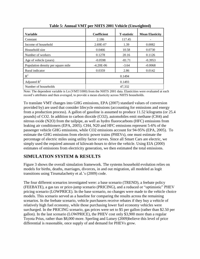
Table 5: Annual VMT per NHTS 2001 Vehicle (Unweighted)

Variable Coefficient T-statistic Mean Elasticity

Constant 2.186 117.45 -

Income of household 2.69E-07 1.39 0.0082

Household size 0.0466 10.58 0.0730

Number of workers 0.1278 20.16 0.1126

Age of vehicle (years) -0.0598 -81.71 -0.3953

Population density per square mile -4.20E-06 -3.64 -0.0068

Rural indicator 0.0359 2.86 0.0142

R2 0.1494

Adjusted R2 0.1493

Number of households 47,332

Note: The dependent variable is Ln (VMT/1000) from the NHTS 2001 data. Elasticities were evaluated at each

record‟s attributes and then averaged, to provide a mean elasticity across NHTS households.

To translate VMT changes into GHG emissions, EPA (2007) standard values of conversion

provided by) are used that consider lifecycle emissions (accounting for emissions and energy

from a production process). A gallon of gasoline is assumed to produce 11.52 kilograms (or 25.4

pounds) of CO2. In addition to carbon dioxide (CO2), automobiles emit methane (CH4) and

nitrous oxide (N2O) from the tailpipe, as well as hydro fluorocarbons (HFC) emissions from

leaking air conditioners (EPA, 2005). CH4, N20 and HFC emissions represent 5-6% of the

passenger vehicle GHG emissions, while CO2 emissions account for 94-95% (EPA, 2005). To

estimate the GHG emissions from electric power trains (PHEVs), one must estimate the

percentage of electric miles using utility factor curves. Since all Smart Cars are electric, we

simply used the required amount of kilowatt-hours to drive the vehicle. Using EIA (2000)

estimates of emissions from electricity generation, we then estimated the total emissions.

SIMULATION SYSTEM & RESULTS

Figure 3 shows the overall simulation framework. The systems household evolution relies on

models for births, deaths, marriages, divorces, in and out migration, all modeled as logit

transitions using Tirumalachetty et al.‟s (2009) code.

The four different scenarios investigated were: a base scenario (TREND), a feebate policy

(FEEBATE), a gas tax or price-jump scenario (PRICING), and a reduced or “optimistic” PHEV

pricing scenario (LOWPRICE). In the base scenario, no changes were made to the vehicle choice

models. This scenario served as a baseline for comparing the results across the remaining

scenarios. In the feebate scenario, vehicle purchasers receive rebates if they buy a vehicle of

relatively high fuel economy, while those purchasing lower fuel economy vehicles were

surcharged. In the PRICING scenario, gas prices were set to $5 per gallon (rather than $2.50 per

gallon). In the last scenario (LOWPRICE), the PHEV cost only $3,900 more than a regular

Toyota Prius, rather than $8,000 more. Sperling and Lutsey (2009)believe this level of price

differential is reasonable, once supply of and demand for PHEVs grow.

A full household evolution simulation for ten percent of the population (52,399 households) took

2 days on a 3GB RAM and 2.4 GHz processor to obtain future years‟ demographics. Vehicle

fleet composition and usage models were then run, requiring 10 hours per scenario on the same

personal computer. Average (real) household income during the period of interest is predicted to

rise steadily with an average of 1.1% per year, even though average household size falls slightly

over the 25-year period, by 3.3%. These results are in line with trend statistics provided by

NHTS (2001). The number of households and persons are simulated to grow by 109% and 70%,

respectively, over the 25-year period. With respect to vehicle ownership and GHG emissions,

simulations suggest interesting differences across scenarios. These are explained in detail below.

Figure 3: Overall Modeling Framework

Vehicle Choices

In IEA‟s (2008) recent report on the future of hybrid and road electric vehicles, HEVs are

estimated to represent just 2.2% of all year-2008 car sales. According to this works‟ TREND

scenario, the sale of HEVs and PHEVs will represent 10% of the market share by 2034. These

results are in line with IEA (2009) expectations, which reports that the lack of public awareness

regarding alternative fuel vehicles, the reluctance shown by vehicle manufacturers, and the

conflicting interests of government and vehicle buyers lead to single-digit shares through 2015.

With regard to Smart Cars (BEVs), IEA‟s (2008) states that the market for battery electric

vehicles is small and acceptance of two-wheel electric vehicles might prepare the market for

advanced electric-powered designed vehicles. Our results indicate, however, that Smart Cars

may well have a very small share (2.3% in simulation-year 25, or 2034) in the overall mix of

Austin‟s future vehicles, under the TREND scenario.

Table 5 provides year 2034 predictions. The LOWPRICE scenario, which models the impact of

a $4,100 reduction in the base price of PHEVs, simulated the PHEV‟s market share to rise to

6.14% by 2034. Three-vehicle households are estimated to be the highest adopters of HEVs

(17.1% of the three vehicle households own at least one PHEV in their fleet), and two-vehicle

households are the highest adopters of PHEVs (16.7%). These results complement the work of

Gallagher and Muehlegger (2008), who found that 6%, 27% and 36% of current U.S. HEV sales

can be respectively attributed to tax incentives, rising gasoline prices, and social preferences.

The $5-per-gallon (PRICING) scenario was estimated to have only a minor impact on the

composition of vehicles owned, with slight reductions in the share of Smart Cars, PHEVs and

vans, alongside higher shares of compact and subcompact cars (20%), SUVs/CUVs and HEVs.

More specifically, 5 to 20% of the two-vehicle households (with the share rising over time)

chose to acquire a HEV in each of the model years, under this scenario. Decreasing shares of

PHEV presence are simulated over time, in four-vehicle households, falling from roughly 3.1%

to 2.5%.

Under the FEEBATE policy, household auto ownership levels are predicted to rise, more so

than in any other scenario, thanks to the effective reduction in efficient-vehicle prices. As

expected, there is a preference for more fuel efficient vehicles under this scenario (relative to

TREND), resulting in roughly a 19% market share for HEVs and PHEVs by 2034. Nevertheless,

purchases of less efficient vehicles remains solid and the strategy‟s revenues are estimated to

exceed payouts by 12%, 33% and 37% in years 2014, 2024 and 2034, with total receipts rising

(at a decreasing rate) over time (at roughly 3.4% a year). Under the feebate scenario, the market

share of compact cars and subcompact cars is predicted to rise, every year, while shares of

SUVs, CUVs and pickup trucks fall. Results from the feebate scenario suggest that an increasing

share of the two-vehicle and three-vehicle households will hold at least one HEV and PHEV in

their vehicle fleet, while HEV and PHEV shares may fall very slightly, across four-vehicle

households. The feebate scenario yielded the highest share of HEVs and PHEVs, as compared to

the other scenarios modeled.

Table 5: Vehicle Fleet Composition Predictions (%) for the Year 2034

Base Scenario

(TREND)

Optimistic PHEV

Pricing

(LOWPRICE)

Feebates

(FEEBATE)

Gas at $5/gallon

(PRICING)

Smart Car 54,290 2.33 48,099 2.03 64,304 2.69 55,692 2.38

PHEV 57,137 2.45 145,847 6.14 112,185 4.69 55,799 2.38

HEV 175,356 7.51 152,161 6.41 345,409 14.43 180,728 7.71

Compact car 157,159 6.73 150,287 6.33 153,787 6.42 131,872 5.62

Subcompact 296,519 12.70 283,715 11.95 289,597 12.10 329,022 14.03

Midsize car 185,536 7.95 183,235 7.72 187,386 7.83 194,694 8.30

Large car 224,706 9.62 225,886 9.51 203,782 8.51 219,211 9.35

Luxury car 167,889 7.19 218,013 9.18 188,399 7.87 169,336 7.22

Van 195,708 8.38 193,280 8.14 198,613 8.30 155,943 6.65

Pickup truck 307,010 13.15 288,051 12.13 207,699 8.68 279,826 11.93

SUV 276,504 11.84 260,235 10.96 237,212 9.91 338,833 14.45

CUV 236,855 10.15 225,886 9.51 205,292 8.58 233,865 9.97

Average

vehicle

ownership

2.31

2.29

2.37

2.32

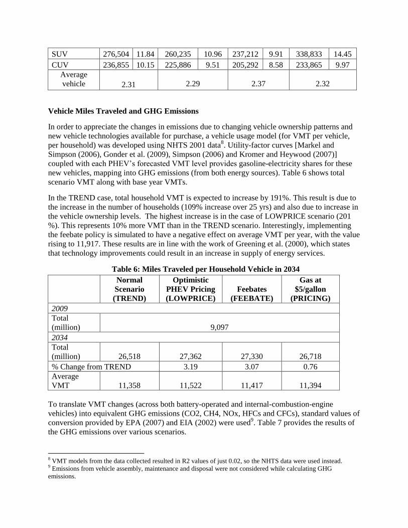
Vehicle Miles Traveled and GHG Emissions

In order to appreciate the changes in emissions due to changing vehicle ownership patterns and

new vehicle technologies available for purchase, a vehicle usage model (for VMT per vehicle,

per household) was developed using NHTS 2001 data8. Utility-factor curves [Markel and

Simpson (2006), Gonder et al. (2009), Simpson (2006) and Kromer and Heywood (2007)]

coupled with each PHEV‟s forecasted VMT level provides gasoline-electricity shares for these

new vehicles, mapping into GHG emissions (from both energy sources). Table 6 shows total

scenario VMT along with base year VMTs.

In the TREND case, total household VMT is expected to increase by 191%. This result is due to

the increase in the number of households (109% increase over 25 yrs) and also due to increase in

the vehicle ownership levels. The highest increase is in the case of LOWPRICE scenario (201

%). This represents 10% more VMT than in the TREND scenario. Interestingly, implementing

the feebate policy is simulated to have a negative effect on average VMT per year, with the value

rising to 11,917. These results are in line with the work of Greening et al. (2000), which states

that technology improvements could result in an increase in supply of energy services.

Table 6: Miles Traveled per Household Vehicle in 2034

Normal

Scenario

(TREND)

Optimistic

PHEV Pricing

(LOWPRICE)

Feebates

(FEEBATE)

Gas at

$5/gallon

(PRICING)

2009

Total

(million) 9,097

2034

Total

(million) 26,518 27,362 27,330 26,718

% Change from TREND 3.19 3.07 0.76

Average

VMT 11,358 11,522 11,417 11,394

To translate VMT changes (across both battery-operated and internal-combustion-engine

vehicles) into equivalent GHG emissions (CO2, CH4, NOx, HFCs and CFCs), standard values of

conversion provided by EPA (2007) and EIA (2002) were used9. Table 7 provides the results of

the GHG emissions over various scenarios.

8 VMT models from the data collected resulted in R2 values of just 0.02, so the NHTS data were used instead.

9 Emissions from vehicle assembly, maintenance and disposal were not considered while calculating GHG

emissions.

Table 7: Greenhouse Gas Emissions from Transportation in 2034

Normal

Scenario

(TREND)

Optimistic PHEV

Incremental

Pricing

(LOWPRICE)

Feebates

(FEEBATE)

Gas at $5/gallon

(PRICING)

2009

VOC and

NOX 518

CO2e 9,842

2034

VOC and

NOX 1,720 1,655 1,623 1,719

CO2e 32,854 31,855 31,167 32,832

% Change of CO2e from

TREND -3.04 -5.13 -0.07

% Change of VOC and NOX

from TREND -3.78 -5.64 -0.06

SUMMARY AND CONCLUSIONS

Vehicle ownership and use is fundamental to understanding and anticipating travel choices. This

study developed a microsimulation model for estimating future greenhouse gas emissions from

household and vehicle fleet evolution. A vehicle choice survey was conducted to appreciate

vehicle ownership patterns and personal opinions of various technologies under multiple

scenarios in the Austin region. A variety of revealed and stated preference questions provide

insight into respondents‟ vehicle choice and attitudes towards potential policies and vehicle

technologies.

Vehicle fleet evolution patterns and greenhouse gas emissions from Austin‟s personal vehicle

fleet were estimated under various scenarios, and the forecasts illuminate several trends and

policy possibilities. Ownership shares of PHEVs, HEVs and Smart Cars are of great interest to

manufacturers and policymakers, and these shares are relatively variable across scenarios, due to

their lower starting counts. Most importantly, due to the missing fuel cost and fuel economy

variables in the VMT and stated preference vehicle choice models, the results obtained in the

PRICING scenario are not consistent with intuition (in terms of magnitude). But this is being

addressed through model refinements.

In the LOWPRICE scenario, fleet VMT is estimated to be 3.09% higher than TREND, while

CO2 emissions are estimated to fall by 3.01%, thanks to higher levels of HEV, PHEV and luxury

car shares and lower vehicle ownership levels.

In the PRICING scenario, gas prices were set to $5 per gallon (rather than the TREND scenario‟s

$2.5/gallon), yet use levels (and total VMT) remained similar to the TREND scenario. This is no

doubt due to the fact that vehicle choice model and the vehicle usage model do not have a

parameter corresponding to fuel economy (thanks to statistical insignificance [in the ownership

models] and unavailability of this covariate [in the NHTS data set]). Under this scenario, 20% of

the light-duty/personal fleet is predicted to be small cars (compact and subcompact cars) by 2034

(rather than the 14% found in the recent Austin Travel Survey).

The FEEBATE scenario‟s results are also quite interesting: while its vehicle ownership and use

levels are predicted to be comparatively higher, across all scenarios, its GHG emissions levels

are expected to be slightly lower than the TREND, PRICING and LOWPRICE scenarios. It is

expected to generate net revenues of $871 per new vehicle sold and facilitate mobility while

reducing overall CO2 emissions (though only slightly, by 5.13 % of light-vehicle fleet emissions,

relative to trend).

Most respondents (63% [weighted share]) indicated support for a feebate policy, and most (56%)

claimed they would consider purchasing a PHEV (if it were to cost $6,000 more than its internal

combustion counterpart). So such policy changes may well be possible, along with a faster fleet

turnover towards more fuel efficient vehicles. The evolution of passenger fleets remains to be

seen, however; new technologies, pricing, marketing and various policies may prove critical to

the path we take.

Some Final Suggestions

There are several areas that remain open for further exploration. More realistic scenarios with

more diverse vehicle options in tandem with careful in-person interviews can help ensure more

realistic response on stated preference questions, particularly for vehicles that do not yet exist.

Recognition of vehicle use patterns (vis-à-vis the vehicle choice decision) along with unexpected

vehicle loss (due to crashes and theft, for example) would enhance the information content and

reliability of results. Greater reliance on past/revealed transactions data could also be useful.

Finally, information about driving habits, travel behavior, frequency and length of long-distance

trips affect the use, fuel economy and emissions from household vehicle fleets may be critical to

PHEV adoption feasibility, greenhouse gas impacts, and other attributes of great interest to local

and global communities. New survey instruments and first-hand data collection may be key to

addressing such questions.

ACKNOWLEDGEMENTS

We want to thank the Southwest Region University Transportation Center for financially

supporting this study. We also appreciate the assistance of Ms. Annette Perrone and Ms.

Katherine Kortum for editorial assistance.

REFERENCES

Axsen, J., and K. Kurani. 2008. The Early U.S. Market for PHEVs: Anticipating Consumer

Awareness, Recharge Potential, Design Priorities and Energy Impacts. Institute of Transportation

Studies, University of California, Davis, Research Report UCD-ITS-RR-08-22. Accessed from

http://pubs.its.ucdavis.edu/publication_detail.php?id=1191 on April 12, 2009.

Berkovec, J. 1985. Forecasting Automobile Demand Using Disaggregate Choice Models.

Transportation Research B, 19(4): 315-329.

Berkovec, J., and J. Rust. 1985. A Nested Logit Model of Automobile Holdings for One Vehicle

Households. Transportation Research B, 19(4): 275-285.

Bhat, C.R., S. Sen, and N. Eluru. 2008. The Impact of Demographics, Built Environment

Attributes, Vehicle Characteristics, and Gasoline Prices on Household Vehicle Holdings and

Use. Transportation Research Part B, 43(1): 1-18.

British Broadcasting Corporation BBC (2002) The U.S. and Climate Change. Accessed from

http://news.bbc.co.uk/2/hi/americas/1820523.stm on September 30, 2008.

CalCars. 2003. The California Cars Initiative 2003. Plug-In Hybrids, Palo Alto, California.

Available at http://www.calcars.org/.

Choo, S., and P. Mokhtarian. 2004. What type of vehicle do people drive? The role of attitude

and lifestyle in influencing vehicle type choice. Transportation Research A, 38 (3): 201-222.

Dubin, J. and D. McFadden. 1984. An Econometric Analysis of Residential Appliance Holdings

and Consumption. Econometrica, 52 (2): 345-362.

Energy Information Agency (EIA). 2002. Updated State-level Greenhouse Gas Emission

Coefficients for Electricity Generation 1998-2000. Report No. DOE/EIA-0348. Accessed June

20, 2009.

Environmental Protection Agency (EPA). 2005. Emission Facts: Greenhouse Gas Emissions

from a Typical Passenger Vehicle. Report #: EPA420. Accessed from

http://www.epa.gov/OMS/climate/420f05004.htm on December 21, 2008.

Energy Information Agency (EIA). 2007. Emissions of Greenhouse Gases in the United States

for 2006. Report No. DOE/EIA-0573. Accessed from

http://www.eia.doe.gov/oiaf/1605/ggrpt/pdf/enduse_tbl.pdf on June 28, 2009.

Energy Information Administration (EIA). 2007. Renewable Fuel Standard Program, Chapter 6

Lifecycle Impacts on Fossil Energy and Greenhouse Gases. Accessed from

http://www.epa.gov/otaq/renewablefuels/420r07004chap6.pdf on November 5, 2009.

Espey, M., and S. Nair. 2005. Automobile Fuel Economy: What is it Worth? Contemporary

Economic Policy, 23 (3): 317-323.

Fang, H. 2008. A Discrete-Continuous Model of Households‟ Vehicle Choice and Usage, with

an Application to the Effects of Residential Density. Transportation Research B, 42(9): 736-

758.

Feng, Y., D. Fullerton, and L. Gan. 2005. Vehicle Choices, Miles Driven and Pollution Policies.

Working paper 11553, National Bureau of Economic Research. Accessed from

http://works.bepress.com/cgi/viewcontent.cgi?article=1008&context=don_fullerton on

December 25, 2008.

First Electric Cooperative. 2009. PHEV FAQ 2009.

http://www.firstelectric.coop/content.cfm?id=2107. Accessed on April 21, 2009.

Gallagher, K., and E. Muehlegger. 2008. Giving Green to Get Green? The Effect of Incentives

and Ideology on Hybrid Vehicle Adoption. Working Paper. Available at

http://ksghome.harvard.edu/~emuehle/Research%20WP/Gallagher%20and%20Muehlegger%20

Feb_08.pdf.

Gonder, J., A. Brooker, R. Carlson and J. Smart. 2009. Deriving In-Use PHEV Fuel Economy

Predictions from Standardized Test Cycle Results. Report No. NREL/CP-540-46251.

http://www.nrel.gov/vehiclesandfuels/vsa/pdfs/46251.pdf. Accessed May 16, 2009.

Greening, L., D. L. Greene and C. Difiglio. 2000. Energy Efficiency and Consumption-The

Rebound Effect - A Survey. Energy Policy, 28: 389-401.

Heffner, R., K. Kurani, and T. Turrentine. 2007. Symbolism in Early Markets for Hybrid Electric

Vehicles. Technical Paper, Institute of Transportation Studies, University of California, Davis.

Available at http://pubs.its.ucdavis.edu/download_pdf.php?id=1063.

International Energy Agency (IEA). 2008. Outlook for Hybrid and Electric Vehicles. Accessed

from http://www.ieahev.org/pdfs/ia-hev_outlook_2008.pdf on September 17, 2009.

Kitamura, R., T. F. Golob, T. Yamamoto and G. Wu. 2000. Accessibility and Auto Use in

aMotorized Metropolis. Proceedings at the 79th

Transportation Research Board Annual Meeting,

Washington, DC.

Kockelman, K.M. and Y. Zhao. 2000. Behavioral Distinctions: The use of Light-Duty Trucks

and Passenger Cars. Journal of Transportation and Statistics, 3(3): 47-60.

Kumar, S. 2007. Microsimulation of Household and Firm Behaviors: Coupled Models of Land

Use and Travel Demand in Austin, Texas. Master„s Thesis. Department of Civil Engineering,

The University of Texas at Austin.

Kurani, K., and T. Turrentine. 2004. Automobile Buyer Decisions about Fuel Economy and Fuel

Efficiency. Final Report to United States Department of Energy and the Energy Foundation.

Accessed from http://pubs.its.ucdavis.edu/download_pdf.php?id=193 on October 24, 2008.

Kurani, K., R. Heffner and T. Turrentine. 2009. Driving Plug-In Hybrid Electric Vehicles:

Reports from U.S. Drivers of HEVs converted to PHEVs. Proceedings of the 88th

Transportation

Research Board Annual Meeting, Washington, DC.

Langer, A., N. Miller. (2008). Automobile Prices, Gasoline Prices, and Consumer Demand for

Fuel Economy. Economic Analysis Group Discussion Paper, University of California, Berkeley.

Accessed from

http://drwww.wm.edu/as/economics/research/seminars/seminardocs/Miller_Langer.pdf on

September 28, 2009.

Lave, C. A., and K. Train. 1979. A Disaggregate Model of Auto-Type Choice. Transportation

Research A, 13(1): 1-9.

Lemp, J., and K. Kockelman. 2008. Quantifying the External Costs of Vehicle Use: Evidence

from America‟s Top Selling Light-Duty Models. Transportation Research D, 13: 491-504.

Mannering, F., and C. Winston. 1985. A Dynamic Empirical Analysis of Household Vehicle

Ownership and Utilization. Rand Journal of Economics, 16(2): 215-236.

Mannering, F., C. Winston, and W. Starkey. 2002. An Exploratory Analysis of Automobile

Leasing by US Households. Journal of Urban Economics, 52(1): 154–176.

Manski, C. F., and L. Sherman. 1980. An Empirical Analysis of Household Choice among Motor

Vehicles. Transportation Research A, 14(5/6): 349-366.

Markel, T. 2006a. Plug-In HEV Vehicle Design Options and Expectations. Report No.

NREL/PR-40630 http://www.nrel.gov/docs/fy06osti/40630.pdf. Accessed April 14, 2009.

Markel, T. 2006b. Plug-In HEV: Current Status, Long-Term Prospects and Key Challenges

Report No. NREL/PR-40239 http://www.nrel.gov/docs/fy06osti/40239.pdf. Accessed April 14,

2009.

Markel, T., and A. Simpson. 2006. Plug-In Hybrid Electric Vehicle Energy Storage System

Design. Report No. NREL/CP-540-39614

http://www.nrel.gov/vehiclesandfuels/vsa/pdfs/39614.pdf. Accessed May 16, 2009.

Mohammadian, A., and E. J. Miller, 2003a. An Empirical Investigation of Household Vehicle

Type Choice Decisions. Transportation Research Record, 1854: 99-106.

Mohammadian, A., and E. J. Miller, 2003b. Dynamic Modeling of Household Automobile

Transactions. Transportation Research Record, 1831: 98-105.

Musti, S., K. Kortum and K. Kockelman. 2009. Household Energy Use and Travel:

Opportunities for Behavioral Change. Presented at the 12th TRB National Transportation

Planning Applications Conference, in Houston, Texas. Accessed from

http://www.caee.utexas.edu/prof/kockelman/public_html/TRB10EnergySurvey.pdf on June 30,

2009.

National Household Travel Survey (NHTS). 2001. National Data on the Travel Behavior of

American Public. Accessed from http://nhts.ornl.gov/download.shtml on August 22, 2009.

Potoglou, D., and P. Kanaroglou. 2007. Household Demand and Willingness to Pay for Clean

Vehicles. Transportation Research D, 12 (4): 264-274.

Prillwitz, J., S. Harms, and M. Lanzendorf. 2008. Impact of Life Course Events on Car

Ownership. Poster for the 85th Annual Meeting of the Transportation Research Board,

Washington, D.C., January 22-26, 2006.

Puller, S.L., and L.A. Greening. 1999. Household Adjustment to Gasoline Price Change: An

Analysis Using 9 Years of US Survey Data. Energy Economics, 21(1): 37-52.

Roorda, M., A. Mohammadian, and E.J. Miller. 2000. Toronto Area Car Ownership Study: A

Retrospective Interview and its Applications. Transportation Research Record, 1719: 69-76.

Roy, R. 1947. La Distribution du Revenu Entre Les Divers Biens. Econometrica, 15: 205-225.

Simpson, A. 2006. Cost-Benefit Analysis of Plug-In Hybrid Electric Vehicle Technology. Report

No. NREL/CP-540-40485. http://www.nrel.gov/vehiclesandfuels/vsa/pdfs/40485.pdf. Accessed

April 14, 2009.

Small, K. A., and K. van Dender. 2007. Fuel Efficiency and Motor Vehicle Travel: The

Declining Rebound Effect. Energy Journal, 28(1): 25-51.

Small, K. A., and C. Kazimi. 1995. On the Costs of Air Pollution from Motor Vehicles. Journal

of Transport Economics and Policy, 29(1): 7-32.

Smith, C., G. Spitz, M. Fowler and T. Seely. 2009a. Internet Access: Is Everyone Online Yet and

Can We Survey Them There? Presented at the 12th TRB National Transportation Planning

Applications Conference, in Houston, Texas.

Smith, C., M. Fowler, E. Greene and C. Nielson. 2009b. Carbon Emissions and Climate Change:

A Study of Attitudes and their Relationship with Travel Behavior. Presented at the 12th TRB

National Transportation Planning Applications Conference, in Houston, Texas.

Sperling, D. and N. Lutsey. 2009. Energy Efficiency in Passenger Transportation. The Bridge,

39(2): 22-30.

Train, K. 1980. A Structured Logit Model of Auto Ownership and Mode Choice. Review of

Economic Studies, 47: 357-370.

Tirumalachetty, S. 2009. Microsimulation of Household and Firm Behaviors: Anticipation of

Greenhouse Gas Emissions- in Austin, Texas. Master„s Thesis. Department of Civil Engineering,

The University of Texas at Austin.

Tirumalachetty, S., K. Kockelman, and S. Kumar. 2009. Micro-Simulation Models of Urban

Regions: Anticipating Greenhouse Gas Emissions from Transport and Housing in Austin, Texas.

Proceedings of the 88th

Annual Meeting of the Transportation Research Board, Washington,

D.C.

Ward‟s. 2007. Ward’s Automotive Yearbook 2007. Ward‟s Communications, Detroit, Michigan.

Zhao, Y. and K. M. Kockelman. 2002. Household Vehicle Ownership by Vehicle Type:

Application of a Multivariate Negative Binomial Model. Proceedings of the Transportation

Research Board‟s 81st Annual Meeting, Washington, DC.