Expert Systems with Applications 39 (2012) 3603–3610

Contents lists available at SciVerse ScienceDirect

Expert Systems with Applications

journal homepage: www.elsevier .com/locate /eswa

Evolutionary algorithm for stochastic job shop scheduling with randomprocessing time q

Shih-Cheng Horng a, Shieh-Shing Lin b, Feng-Yi Yang c,⇑a Department of Computer Science and Information Engineering, Chaoyang University of Technology, Taiwan, ROCb Department of Electrical Engineering, St. John’s University, Taiwan, ROCc Department of Biomedical Imaging and Radiological Sciences, National Yang-Ming University, Taiwan, ROC

a r t i c l e i n f o a b s t r a c t

Keywords:Stochastic job shop schedulingEvolutionary strategyOrdinal optimizationSimulation optimizationDispatching rule

0957-4174/$ - see front matter � 2011 Elsevier Ltd. Adoi:10.1016/j.eswa.2011.09.050

q This work was partially supported by National Scunder Grant NSC100-2221-E-324-006.⇑ Corresponding author. Address: No. 155, Sec. 2

Taiwan, ROC. Tel.: +886 2 28267281; fax: +886 2 282E-mail addresses: schong@cyut.edu.tw (S.-C. Horng

Lin), fyyang@ym.edu.tw (F.-Y. Yang).

In this paper, an evolutionary algorithm of embedding evolutionary strategy (ES) in ordinal optimization(OO), abbreviated as ESOO, is proposed to solve for a good enough schedule of stochastic job shop sched-uling problem (SJSSP) with the objective of minimizing the expected sum of storage expenses and tardi-ness penalties using limited computation time. First, a rough model using stochastic simulation withshort simulation length will be used as a fitness approximation in ES to select N roughly good schedulesfrom search space. Next, starting from the selected N roughly good schedules we proceed with goal soft-ening procedure to search for a good enough schedule. Finally, the proposed ESOO algorithm is applied toa SJSSP comprising 8 jobs on 8 machines with random processing time in truncated normal, uniform, andexponential distributions. The simulation test results obtained by the proposed approach were comparedwith five typical dispatching rules, and the results demonstrated that the obtaining good enough sche-dule is successful in the aspects of solution quality and computational efficiency.

� 2011 Elsevier Ltd. All rights reserved.

1. Introduction Research about scheduling problems focusing on random process-

In the last two decades, a great deal of research works has beenconducted on job shop scheduling problem (JSSP). Many ap-proaches are used in dealing with JSSP, such as analytical tech-niques, rule-based approaches and meta-heuristic algorithms(Chakraborty, 2009). Analytical techniques can get the optimal ornear-optimal solution, but they cannot describe the stochasticcharacteristic of the manufacture system (Fattahi, Mehrabad, &Jolai, 2007). Rule-based approaches are widely used in practice be-cause of their simplicity and effectiveness (Sule, 2007). However,there is no single rule that is the best under all possible conditions.Meta-heuristic algorithms can get the near-optimal solution, but itconsumes much computation time when the scheduling problemsbecome complex (Zhang & Wu, 2010).

Most of the job shop scheduling problems are the stochasticscheduling ones in real manufacture system. Stochastic job shopscheduling problem (SJSSP) is a NP-hard problem, which reflectsthe real-world situations and tends to suffer from its uncertain fea-ture. The literature of the stochastic job shop scheduling is notablysparser than the literature of the deterministic job shop scheduling.

ll rights reserved.

ience Council in Taiwan, ROC

, Li-Nong St., Taipei 11221,01095.), sslin@mail.sju.edu.tw (S.-S.

ing time is one of the newest issues that have been interested re-cently with regard to the need of flexible manufacturing system. Ascheduling method based on variable neighborhood search (VNS)was introduced in (Zandieh & Adibi, 2010) to address a dynamic JSSPthat considers random job arrivals and machine breakdowns. Rennacreated the schedule by a pheromone-based approach and carriedout by a multi-agent architecture (Renna, 2010). Zhou et al. pro-posed an ant colony optimization algorithm (ACO) with three levelsof machine utilizations, three different processing time distribu-tions, and three different performance measures for solving dy-namic JSSP (Zhou, Nee, & Lee, 2009). A hybrid method that utilizesa neural network approach is developed in (Tavakkoli-Moghaddam,Jolai, Vaziri, Ahmed, & Azaron, 2005) to generate initial feasible solu-tions, then a simulated annealing (SA) algorithm is applied to im-prove the quality and performance of initial solutions to obtain anear-optimal solution. In Lei (2010), an efficient decomposition-integration genetic algorithm is developed to minimize themaximum fuzzy completion time. Gu et al. proposed a competitiveco-evolutionary quantum genetic algorithm (GA) for solving SJSSPwith the objective to minimize the expected makespan (Gu, Gu,Cao, & Gu, 2010), but negative or zero processing time comes fromthe normal distribution as a probability distribution function maynot be the best way reflecting the stochastic nature of processingtime. Gholami and Zandieh integrated simulation into genetic algo-rithm to the dynamic scheduling of a flexible job shop with theobjective to minimize the expected makespan and expected mean

3604 S.-C. Horng et al. / Expert Systems with Applications 39 (2012) 3603–3610

tardiness (Gholami & Zandieh, 2009). In Gu, Gu, and Gu (2009), a par-allel quantum genetic algorithm is proposed for SJSSP with theobjective of minimizing the expected makespan, where the process-ing times are subjected to independent normal distributions.

All the above methods suffer from lengthy computation times,because evaluating the objective of a schedule is already verytime-consuming not even mention the extremely slow convergenceof the heuristic techniques in searching through a huge search space.To overcome the drawback of consuming much computation timefor complex scheduling problems, we propose an evolutionary algo-rithm of embedding the evolutionary strategy (ES) in ordinal optimi-zation (OO), abbreviated as ESOO, to solve for a good enough feasibleschedule within a reasonable amount of time. The key idea of ESOOalgorithm is to narrow the search space step by step or gradually re-strict the search through iterative use of ordinal optimization (Ho,Zhao, & Jia, 2007; Shen, Ho, & Zhao, 2009). It is in the spirit of tradi-tional hill climbing except instead of moving from one point to pointin the search space, ESOO algorithm moves from one subset to an-other. The SJSSP is formulated as a constrained stochastic simulationoptimization problem that possesses a huge search space and ismost suitable for demonstrating the validity of the proposed ESOOalgorithm. To overcome the drawback of negative or zero processingtime resulting from probability distribution function, we consider aSJSSP with stochastic processing time in truncated normal, uniform,and exponential distributions. Because the use of both earliness andtardiness penalties gives rise to a nonregular performance measure,storage expenses of earliness and tardiness penalties will be servedas the objective function of our optimization problem. Therefore, thepurpose of this paper is to determine a good enough schedule withthe objective of minimizing expected sum of storage expenses andtardiness penalties using limited computation time. The developedmathematical formulation is the first contribution of this paper,which can be used for job shop manufacturing systems with randomprocessing time and various cost penalties and expenses.

The proposed ESOO algorithm is another contribution of this pa-per, which consists of exploration and exploitation stage. Theexploration stage uses ES to efficiently select N excellent solutionsfrom the search space, where the fitness function is evaluated witha rough model. To ensure generating of feasible schedules, a prece-dence-based permutation encoding and a repair operator are uti-lized in the processes of ES. The exploitation stage composes ofmultiple phases, which allocate the computing resource and bud-get by iteratively and adaptively selecting the candidate solutionset. At each phase, remaining solutions are evaluated and someof them are eliminated, and the solution obtained in the last phaseis the good enough schedule that we seek.

The rest of this paper is organized as follows. In Section 2, wepresent a mathematical formulation of a general SJSSP and de-scribe the difficulty of the problem. In Section 3, we illustrate theproposed ESOO algorithm for finding a good enough schedule fromthe search space. In Section 4, the proposed algorithm is applied toa SJSSP comprising 8 jobs on 8 machines with random processingtime in truncated normal, uniform, and exponential distributions.We show the test results of applying the proposed approach anddemonstrate the solution quality by comparing with those ob-tained by five typical dispatching rules. We also provide the perfor-mance analysis of our approach to justify the global goodness ofthe obtained solution. Finally, we make a conclusion in Section 5.

2. Stochastic job shop scheduling problem

2.1. Problem statement

We consider a problem of machine scheduling known as thegeneral SJSSP. A set of n jobs is given, denoted as Ji, 1 6 i 6 n. Every

job consists of a sequence of operations, each of which needs to beprocessed during an uninterrupted time period on a given ma-chine. A set of m machines is given, denoted as Mk, 1 6 k 6 m. Eachmachine can process at most one operation at a time. The opera-tion of job Ji processed on machine Mk is denoted as Oi,k,1 6 i 6 n, 1 6 k 6 m. We denote the index of processing sequenceof Oi,k by ai,k, which is given in advance. The random processingtime of Oi,k is denoted by pi,k, which is a random variable followinga given probability distribution function with mean hi,k and vari-ance r2

i;k. For the sake of simplicity in expression, an operationenvironment vector, denoted as ½ai;k; hi;k;r2

i;k�, is used to describethe job shop environment. The due dates, denoted as di, for eachjob Ji are deterministic. If one or more jobs are ready to be pro-cessed on a certain machine and that machine is free, a job willbe chosen and passed on the machine immediately. As a result ofscheduling decisions, job Ji will be assigned a completion time Ci,where Ci is the completion time of the last operation. Let Ti = -max {0,Ci � di} and Ai = max {0,di � Ci} represent the tardinessand earliness of job Ji, respectively.

A schedule specifies the order in which operations are per-formed on machine and can be represented by a random permuta-tion of all Oi,k, 1 6 i 6 n, 1 6 k 6 m. Let H denote the set of feasibleand infeasible schedules without idle times between jobs. A feasi-ble schedule S should satisfy the precedence constraints due to theorder in which the operations need to be done for each of the jobsand also the sequencing constraints to ensure at most one job is per-formed on a machine at a given time. The goal of SJSSP is to find afeasible schedule S e H that minimizes specified objectives and re-spects the following conditions: (i) each machine can process atmost one operation a time; (ii) each job can be performed onlyon one machine at a time; (iii) there are no precedence constraintsamong operations of different jobs; (iv) operations cannot be pre-empted once started.

2.2. Mathematical formulation

In this section, a mathematical model of the general job shopmanufacturing system in stochastic environments is presented. Ifa job Ji is accomplished later than the due date di, a cost penaltyai for each time unit of the delay is paid to the customer. If thejob is accomplished before the due date, the customer does not ac-cept it until the deadline. Thus, the system is compelled to storethe job until the due date and to spend bi per time unit of storage.Taking the economic situation into account, such model covers abroad spectrum of a job shop manufacturing system under randomdisturbances.

The SJSSP for a given operation environment vector ½ai;k; hi;k;r2i;k�

can be formulated as

minS2H

E f ðSÞ ¼Xn

i¼1

aiTi þ biAi

( )ð1Þ

subject to Oi;j satisfy ai;k processing sequence; 8Oi;j 2 S: ð2Þ

where f(S) denotes the sum of tardiness penalties and storage ex-penses; the parameter ai > 0 denotes weight of tardiness penaltyof job Ji (penalty imposed by tardiness), then aiTi denotes tardinesspenalties of job Ji; the parameter bi > 0 denotes the weight of earli-ness penalty of job Ji (penalty imposed by earliness), then biAi de-notes storage expenses of job Ji. Decision maker can determinethe values of tardiness weight and earliness weight based on theeconomic situation. In the case of high machine utilization, the stor-age cost is small relative to the cost of unused production capacity.However, for low machine utilization, deliberate delay of finishingthe job may be more economic. Therefore, the expected sum of tar-diness penalties and storage expenses, E[f(S)], will serve as theobjective function of our optimization problem. Precedence

S.-C. Horng et al. / Expert Systems with Applications 39 (2012) 3603–3610 3605

constraints (2) ensure that the processing sequence of operations ineach job corresponds to the predetermined order. Any feasible solu-tion satisfies constraints (2) is called a feasible schedule.

The objective of this optimization problem is to find a feasibleschedule S that minimizes the expected sum of storage expensesand tardiness penalties from search space H while satisfying pre-cedence constraints. Apparently the above optimization problem isa constrained stochastic simulation optimization problem withhuge search space H. Since simulation can effectively describethe characteristic of operations, a simulation methodology can beused to evaluate the objective value. The principle of simulationmethod is that the analytical objective function is replaced by sim-ulation models. However, to evaluate the true objective value of afeasible schedule S e H, a stochastic simulation of infinite replica-tions is needed to perform. Although infinite replications of simu-lation will make the objective value of (1) stable, in fact, this ispractically impossible. Therefore, depending on the number of rep-lications, (1) can be reformulated as follows:

minS2H

FðSÞ ¼ 1L

XL

l¼1

Xn

i¼1

½aiTliðSÞ þ biA

liðSÞ�

( ); ð3Þ

where L denotes the simulation length, i.e. number of replications,Tl

iðSÞ and AliðSÞ denote the tardiness and earliness of job Ji on the

lth replication of a feasible schedule S, respectively. The samplemean of objective value, F(S), is the average sum of tardiness penal-ties and storage expenses of a feasible schedule S when the simula-tion length is L. Thus, sufficiently large L will make the sample meanof objective value, F(S), sufficiently stable. Let Le = 105 represent thesufficiently large L. In the sequel, the exact model of (3) is defined aswhen the simulation length L = Le. For the sake of simplicity inexpression, let Fe(S) denote the sample mean of objective valuefor a feasible schedule S computed by exact model.

2.3. Difficulty of the problem

Since the job’s processing time fluctuates stochastically at eachmachine of SJSSP, so the process sequences of jobs on each machinecannot be predefined. Even if the sequence has been predefined, itwould become invalidation due to the change of the job’s actualprocess time. Analytical techniques can only be applied to specificcases in job shop scheduling problems with random processingtime (Fattahi et al., 2007). Simulation optimization has a powerfulmodeling and optimization capabilities, so it suited to solve thisconstrained stochastic simulation optimization problem (Keskin,Melouk, & Meyer, 2010; Li, Sava, & Xie, 2009). Due to computationalintractability of objective value, it is unrealistic to optimally solve aSJSSP in reasonable time. Recently, several heuristic searchmethods including the ant colony optimization (ACO) method(Zhou et al., 2009), the simulated annealing (SA) method(Tavakkoli-Moghaddam et al., 2005), and the genetic algorithm(GA) (Gholami & Zandieh, 2009; Gu et al., 2009, 2010; Lei, 2010)have been successfully applied to SJSSP. Despite the success of sev-eral applications of the above heuristic methods, many technicalhurdles and barriers to broader application remain as indicated inDréo, Pétrowski, Siarry, and Taillard (2006). Chief among them isspeed, because using the simulation to evaluate the objective valuefor a given schedule is already computationally expensive not evenmention the search of the best schedule provided that the searchspace is huge. The difficulty of SJSSP makes it very hard for conven-tional search-based methods to find near-optimal schedule in rea-sonable time. Furthermore, simulation often faces situationswhere variability is an integral part of the problem. Thus, stochasticnoise further complicates the simulation optimization problem.The purpose of this paper is to resolve this constrained stochasticsimulation optimization problem efficiently and effectively.

Accordingly, an ESOO algorithm that combines the superiority ofsimulation and meta-heuristic algorithm is presented in nextsection.

3. Embedding the evolutionary strategy in ordinal optimization

As indicated in OO theory (Ho et al., 2007; Shen et al., 2009), thecomputing resource and budget can be allocated by iteratively andadaptively sample subspaces of a large search space in order to lo-cate good designs with high probability. Using ES as a way to iter-atively select N excellent candidate solutions from a large searchspace is a way to do iterative ordinal optimization. Heuristic meth-ods for obtaining N excellent candidate solutions may depend onhow well one’s knowledge about the considered system. For in-stance in the wafer testing process with discrete threshold vari-ables, Horng and Lin proposed an algorithm based on the OOtheory and engineering intuition to select N excellent discretethreshold vectors (Horng & Lin, 2009). However, the engineeringintuition may work only for specific systems. Thus, to select Nroughly good solutions from H without consuming much compu-tation time, we need to construct a rough model that is computa-tionally easy to approximate E[f(S)] of (1) for a given schedule S,and use an efficient method to select N roughly good schedules.The proposed rough model is constructed basing on a stochasticsimulation with short simulation length, and the selection methodis the (l + k) evolution strategy, abbreviated as (l + k)-ES (Beyer &Schwefel, 2002; Mezura-Montes & Coello, 2008).

3.1. Selecting N roughly good schedules S from H

To avoid an accurate but lengthy stochastic simulation toapproximate E[f(S)] for a given schedule S, a rough model is usedto evaluate F(S). The rough model is constructed basing on a sto-chastic simulation with an appropriate basic number of replica-tions Lr, say 368. For the sake of simplicity in expression, we letFr(S) denote the sample mean of objective value for a given S com-puted by rough model. By the aid of the above objective value (orthe so-called fitness in ES terminology) evaluation model, we canefficiently select N excellent schedules from H using ES. Since ESimproves a pool of populations from iteration to iteration, it shouldbest fit our needs. ES is based on the mechanism of natural selec-tion in biological systems and uses a structured but randomizedway to utilize genetic information in finding a new search direc-tion. The improvement process is accomplished using geneticoperators such as recombination and mutation.

3.1.1. RepresentationIndividual representation is a key factor affecting solution qual-

ity and efficiency of ES. In solving the SJSSP using ES, the first task isto represent a schedule as an individual. Because of the existenceof the precedence constraints, not all the randomly permutationsof operations define feasible schedules. Thus, a precedence-basedpermutation representation is utilized in ES that encodes a sche-dule satisfying the processing sequence of operations in whicheach component corresponds to an operation. For a SJSSP compris-ing 3 jobs on 3 machines, the operation environment vector is gi-ven in Table 1. The due dates of jobs J1, J2 and J3 are 11, 12 and8, respectively. From Table 1, the precedence constraints of jobsJ1, J2 and J3 are that O1,1 precedes O1,2 which precedes O1,3, O2,3 pre-cedes O2,2 which precedes O2,1, and O3,2 precedes O3,1 which pre-cedes O3,3, respectively. An individual containing 9 componentsin ES terminology represents a feasible schedule S, and every sche-dule is encoded by precedence-based permutation. Examples ofthe precedence-based permutation encoding of an individual areshown in Fig. 1. Any individual encoding by precedence-based per-

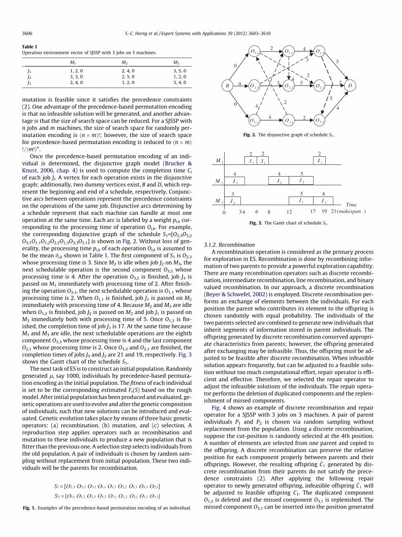
Table 1Operation environment vector of SJSSP with 3 jobs on 3 machines.

M1 M2 M3

J1 1, 2, 0 2, 4, 0 3, 5, 0J2 3, 3, 0 2, 5, 0 1, 2, 0J3 2, 4, 0 1, 2, 0 3, 4, 0

Fig. 2. The disjunctive graph of schedule S1.

Fig. 3. The Gantt chart of schedule S1.

3606 S.-C. Horng et al. / Expert Systems with Applications 39 (2012) 3603–3610

mutation is feasible since it satisfies the precedence constraints(2). One advantage of the precedence-based permutation encodingis that no infeasible solution will be generated, and another advan-tage is that the size of search space can be reduced. For a SJSSP withn jobs and m machines, the size of search space for randomly per-mutation encoding is ðn�mÞ!; however, the size of search spacefor precedence-based permutation encoding is reduced to ðn�mÞ!=ðm!Þn.

Once the precedence-based permutation encoding of an indi-vidual is determined, the disjunctive graph model (Brucker &Knust, 2006, chap. 4) is used to compute the completion time Ci

of each job Ji. A vertex for each operation exists in the disjunctivegraph; additionally, two dummy vertices exist, B and D, which rep-resent the beginning and end of a schedule, respectively. Conjunc-tive arcs between operations represent the precedence constraintson the operations of the same job. Disjunctive arcs determining bya schedule represent that each machine can handle at most oneoperation at the same time. Each arc is labeled by a weight pi,k cor-responding to the processing time of operation Oi,k. For example,the corresponding disjunctive graph of the schedule S1=[O2,3O3,2

O3,1O1,1O1,2O2,2O1,3O3,3O2,1] is shown in Fig. 2. Without loss of gen-erality, the processing time pi,k of each operation Oi,k is assumed tobe the mean hi,k shown in Table 1. The first component of S1 is O2,3

whose processing time is 3. Since M2 is idle when job J2 on M3, thenext schedulable operation is the second component O3,2 whoseprocessing time is 4. After the operation O3,2 is finished, job J3 ispassed on M1 immediately with processing time of 2. After finish-ing the operation O3,1, the next schedulable operation is O1,1 whoseprocessing time is 2. When O1,1 is finished, job J1 is passed on M2

immediately with processing time of 4. Because M2 and M3 are idlewhen O1,2 is finished, job J2 is passed on M2 and job J1 is passed onM3 immediately both with processing time of 5. Once O1,3 is fin-ished, the completion time of job J1 is 17. At the same time becauseM1 and M3 are idle, the next schedulable operations are the eighthcomponent O3,3 whose processing time is 4 and the last componentO2,1 whose processing time is 2. Once O3,3 and O2,1 are finished, thecompletion times of jobs J3 and J2 are 21 and 19, respectively. Fig. 3shows the Gantt chart of the schedule S1.

The next task of ES is to construct an initial population. Randomlygenerated l, say 1000, individuals by precedence-based permuta-tion encoding as the initial population. The fitness of each individualis set to be the corresponding estimated Fr(S) based on the roughmodel. After initial population has been produced and evaluated, ge-netic operations are used to evolve and alter the genetic compositionof individuals, such that new solutions can be introduced and eval-uated. Genetic evolution takes place by means of three basic geneticoperators: (a) recombination, (b) mutation, and (c) selection. Areproduction step applies operators such as recombination andmutation to these individuals to produce a new population that isfitter than the previous one. A selection step selects individuals fromthe old population. A pair of individuals is chosen by random sam-pling without replacement from initial population. These two indi-viduals will be the parents for recombination.

Fig. 1. Examples of the precedence-based permutation encoding of an individual.

3.1.2. RecombinationA recombination operation is considered as the primary process

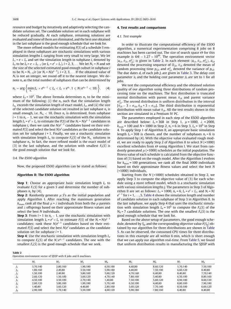
for exploration in ES. Recombination is done by recombining infor-mation of two parents to provide a powerful exploration capability.There are many recombination operators such as discrete recombi-nation, intermediate recombination, line recombination, and binaryvalued recombination. In our approach, a discrete recombination(Beyer & Schwefel, 2002) is employed. Discrete recombination per-forms an exchange of elements between the individuals. For eachposition the parent who contributes its element to the offspring ischosen randomly with equal probability. The individuals of thetwo parents selected are combined to generate new individuals thatinherit segments of information stored in parent individuals. Theoffspring generated by discrete recombination conserved appropri-ate characteristics from parents; however, the offspring generatedafter exchanging may be infeasible. Thus, the offspring must be ad-justed to be feasible after discrete recombination. When infeasiblesolution appears frequently, but can be adjusted to a feasible solu-tion without too much computational effort, repair operator is effi-cient and effective. Therefore, we selected the repair operator toadjust the infeasible solutions of the individuals. The repair opera-tor performs the deletion of duplicated components and the replen-ishment of missed components.

Fig. 4 shows an example of discrete recombination and repairoperator for a SJSSP with 3 jobs on 3 machines. A pair of parentindividuals P1 and P2 is chosen via random sampling withoutreplacement from the population. Using a discrete recombination,suppose the cut-position is randomly selected at the 4th position.A number of elements are selected from one parent and copied tothe offspring. A discrete recombination can preserve the relativeposition for each component properly between parents and theiroffsprings. However, the resulting offspring C1 generated by dis-crete recombination from their parents do not satisfy the prece-dence constraints (2). After applying the following repairoperator to newly generated offspring, infeasible offspring C1 willbe adjusted to feasible offspring C1. The duplicated componentO1,2 is deleted and the missed component O3,1 is replenished. Themissed component O3,1 can be inserted into the position generated

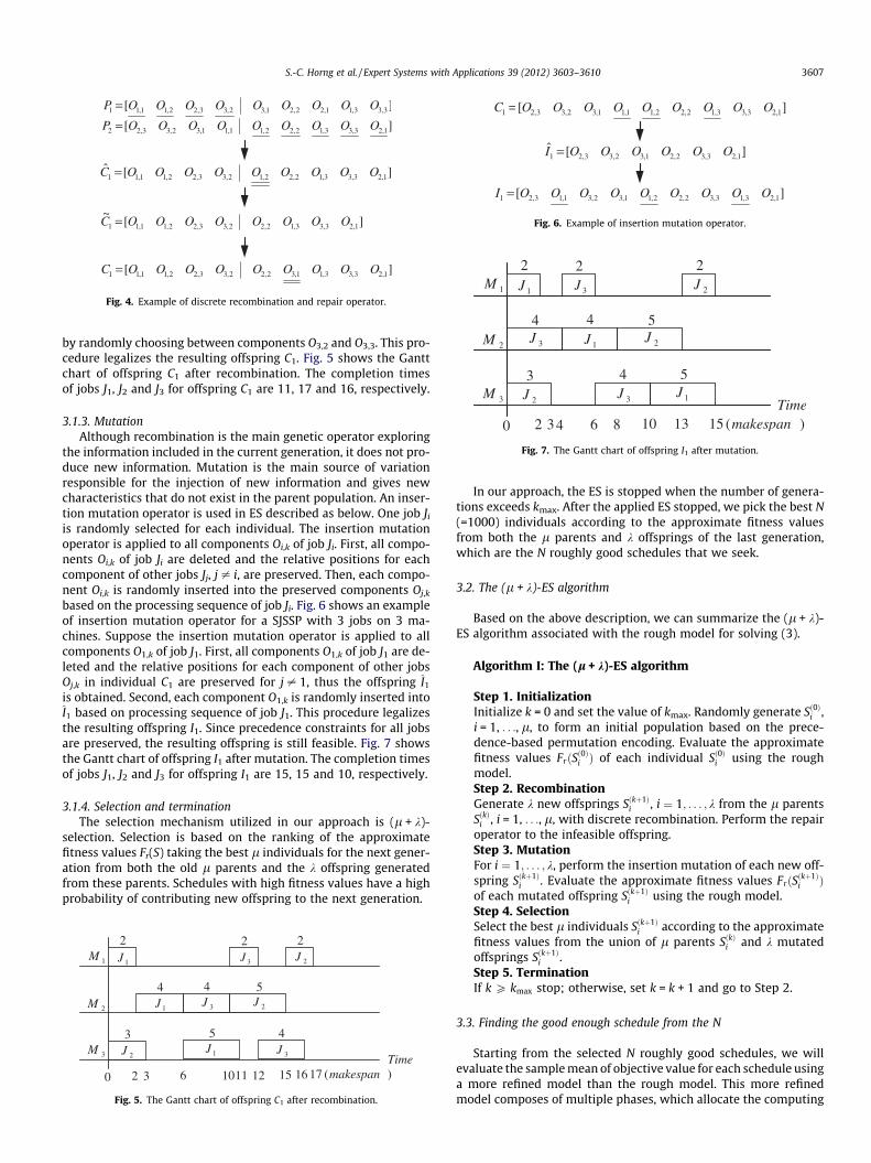
Fig. 4. Example of discrete recombination and repair operator.

Fig. 6. Example of insertion mutation operator.

Fig. 7. The Gantt chart of offspring I1 after mutation.

S.-C. Horng et al. / Expert Systems with Applications 39 (2012) 3603–3610 3607

by randomly choosing between components O3,2 and O3,3. This pro-cedure legalizes the resulting offspring C1. Fig. 5 shows the Ganttchart of offspring C1 after recombination. The completion timesof jobs J1, J2 and J3 for offspring C1 are 11, 17 and 16, respectively.

3.1.3. MutationAlthough recombination is the main genetic operator exploring

the information included in the current generation, it does not pro-duce new information. Mutation is the main source of variationresponsible for the injection of new information and gives newcharacteristics that do not exist in the parent population. An inser-tion mutation operator is used in ES described as below. One job Ji

is randomly selected for each individual. The insertion mutationoperator is applied to all components Oi,k of job Ji. First, all compo-nents Oi,k of job Ji are deleted and the relative positions for eachcomponent of other jobs Jj, j – i, are preserved. Then, each compo-nent Oi,k is randomly inserted into the preserved components Oj,k

based on the processing sequence of job Ji. Fig. 6 shows an exampleof insertion mutation operator for a SJSSP with 3 jobs on 3 ma-chines. Suppose the insertion mutation operator is applied to allcomponents O1,k of job J1. First, all components O1,k of job J1 are de-leted and the relative positions for each component of other jobsOj,k in individual C1 are preserved for j – 1, thus the offspring I1

is obtained. Second, each component O1,k is randomly inserted intoI1 based on processing sequence of job J1. This procedure legalizesthe resulting offspring I1. Since precedence constraints for all jobsare preserved, the resulting offspring is still feasible. Fig. 7 showsthe Gantt chart of offspring I1 after mutation. The completion timesof jobs J1, J2 and J3 for offspring I1 are 15, 15 and 10, respectively.

3.1.4. Selection and terminationThe selection mechanism utilized in our approach is (l + k)-

selection. Selection is based on the ranking of the approximatefitness values Fr(S) taking the best l individuals for the next gener-ation from both the old l parents and the k offspring generatedfrom these parents. Schedules with high fitness values have a highprobability of contributing new offspring to the next generation.

Fig. 5. The Gantt chart of offspring C1 after recombination.

In our approach, the ES is stopped when the number of genera-tions exceeds kmax. After the applied ES stopped, we pick the best N(=1000) individuals according to the approximate fitness valuesfrom both the l parents and k offsprings of the last generation,which are the N roughly good schedules that we seek.

3.2. The (l + k)-ES algorithm

Based on the above description, we can summarize the (l + k)-ES algorithm associated with the rough model for solving (3).

Algorithm I: The (l + k)-ES algorithm

Step 1. InitializationInitialize k = 0 and set the value of kmax. Randomly generate Sð0Þi ,i = 1, . . ., l, to form an initial population based on the prece-dence-based permutation encoding. Evaluate the approximatefitness values FrðSð0Þi Þ of each individual Sð0Þi using the roughmodel.Step 2. RecombinationGenerate k new offsprings Sðkþ1Þ

i , i ¼ 1; . . . ; k from the l parentsSðkÞi , i = 1, . . ., l, with discrete recombination. Perform the repairoperator to the infeasible offspring.Step 3. MutationFor i ¼ 1; . . . ; k, perform the insertion mutation of each new off-spring Sðkþ1Þ

i . Evaluate the approximate fitness values FrðSðkþ1Þi Þ

of each mutated offspring Sðkþ1Þi using the rough model.

Step 4. SelectionSelect the best l individuals Sðkþ1Þ

i according to the approximatefitness values from the union of l parents SðkÞi and k mutatedoffsprings Sðkþ1Þ

i .Step 5. TerminationIf k P kmax stop; otherwise, set k = k + 1 and go to Step 2.

3.3. Finding the good enough schedule from the N

Starting from the selected N roughly good schedules, we willevaluate the sample mean of objective value for each schedule usinga more refined model than the rough model. This more refinedmodel composes of multiple phases, which allocate the computing

3608 S.-C. Horng et al. / Expert Systems with Applications 39 (2012) 3603–3610

resource and budget by iteratively and adaptively selecting the can-didate solution set. The candidate solution set in each subphase willbe reduced gradually. At each subphase, remaining solutions areevaluated and some of them are eliminated, and the best one obtainedin the last subphase is the good enough schedule that we look for.

The more refined models for estimating F(S) of a schedule S em-ployed in these subphases are stochastic simulations with varioussimulation lengths L ranging from very small to very large. We letL1 = e � Lr and set the simulation length in subphase i, denoted byLi, to be Li = e � Li�1 (or Li = ei � Lr), i = 2, 3, . . . We let N1 = N and setthe size of the selected estimated good enough subset in subphase ito be Ni = Ni�1/e (or Ni = N/ei�1), i = 2, 3, . . . If the obtained value ofNi is not an integer, we round off it to the nearest integer. We de-note ns as the total number of subphases that can be determined by

ns ¼ arg minnsðLr � ens�1

6 Le < Lr � ens ;1 6 N=ens�1 < 10Þ� �

; ð4Þ

where Le = 105. The above formula determines ns to be the mini-mum of the following: (i) the ns such that the simulation lengthLns exceeds the simulation length of exact model, Le, and (ii) the sizeof the selected candidate solution set resulted in last subphase ns issmall enough, i.e. Nns < 10. Once ns is determined, from subphasei = 1 to ns � 1, we use the stochastic simulation with the simulationlength Li = ei � Lr to estimate the F(S) of the Ni = N/ei�1 candidates insubphase i, then we rank the N/ei�1 candidates based on their esti-mated F(S) and select the best N/ei candidates as the candidate solu-tion set for subphase i + 1. Finally, we use a stochastic simulationwith simulation length Le to compute Fe(S) of the Nns solutions insubphase ns. In fact, the more refined model is the exact model of(3) in the last subphase, and the solution with smallest Fe(S) isthe good enough solution that we look for.

3.4. The ESOO algorithm

Now, the proposed ESOO algorithm can be stated as follows:

Algorithm II: The ESOO algorithm

Step 1: Choose an appropriate basic simulation length Lr toevaluate Fr(S) for a given S and determine the number of sub-phases ns by (4).Step 2: Randomly generate l S’s as the initial population andapply Algorithm I. After reaching the maximum generationkmax, rank all the final l + k individuals from both the l parentsand k offsprings based on their approximate fitness values andselect the best N individuals.Step 3: From i = 1 to ns � 1, use the stochastic simulation withsimulation length Li = ei � Lr to estimate F(S) of the Ni = N/ei�1

candidates; rank these N/ei�1 candidates based on their esti-mated F(S) and select the best N/ei candidates as the candidatesolution set for subphase i + 1.Step 4: Use the stochastic simulation with simulation length Le

to compute Fe(S) of the N=ens�1 candidates. The one with thesmallest Fe(S) is the good enough schedule that we seek.

Table 2Operation environment vector of SJSSP with 8 jobs and 8 machines.

M1 M2 M3 M4

J1 3,70,140 2,80,160 1,90,180 6,50,100J2 1,80,160 2,40,80 3,50,100 5,90,180J3 1,50,100 2,40,80 3,80,160 5,60,120J4 2,60,120 1,50,100 3,60,120 4,70,140J5 4,50,100 3,50,100 2,70,140 1,40,80J6 2,60,120 3,80,160 1,90,180 5,70,140J7 1,40,80 3,60,120 4,40,80 2,80,160J8 2,90,180 1,70,140 3,50,100 4,60,120

4. Test results and comparisons

4.1. Test example

In order to illustrate the computational efficiency of the ESOOalgorithm, a numerical experimentation comprising 8 jobs on 8machines has been carried out. The size of search space H for thisexample is 64! ¼ 1:27� 1089. The operation environment vector½ai;k; hi;k;r2

i;k� is given in Table 2. In each element ðai;k; hi;k;r2i;kÞ, ai,k

denoted the processing sequence of Oi,k, hi,k denoted the mean ofrandom processing time pi,k, and r2

i;k denoted the variance of pi,k.The due dates di of each job Ji are given in Table 3. The delay costparameter ai and the holding cost parameter bi are set to 1 for alljobs.

We test the computational efficiency and the obtained solutionquality of our algorithm using three distributions of random pro-cessing time on the machines. The first distribution is truncatednormal distribution with parent mean hi,k and parent variancer2

i;k. The second distribution is uniform distribution in the interval[hi,k � 3 � ri,k, hi,k + 3 � ri,k]. The third distribution is exponentialdistribution with mean value hi,k. All the test results shown in thissection are simulated in a Pentium IV PC.

The parameters employed in each step of the ESOO algorithmare described below: Lr = 368 in Step 1, l = 1000, k = 2000,kmax = 100 and N = 1000 in Step 2, ns = 6 in Step 3, Le = 105 in Step4. To apply Step 1 of Algorithm II, an appropriate basic simulationlength Lr = 368 is chosen, and the number of subphases ns = 6 isdetermined by (4). With the objective value evaluated rough mod-el, we are ready to apply Step 2 of Algorithm II to select N (=1000)excellent schedules from H using Algorithm I. We start from ran-domly generated l (=1000) schedules as the initial population. Thefitness value of each schedule is calculated from the objective func-tion of (3) based on the rough model. After the Algorithm I evolvesfor kmax = 100 generations, we rank all the final 3000 individualsbased on their approximate fitness values and select the best N(=1000) individuals.

Starting from the N (=1000) schedules obtained in Step 2, weapply Step 3 to compute the objective value of (3) for each sche-dule using a more refined model, which is a stochastic simulationwith various simulation lengths j. The parameters in Step 3 of Algo-rithm II are set as follows: L1 = 1000, ns = 6, Li = ei � Lr, and Ni = N/ei�1 for i = 1, . . . ,5. Table 4 shows the simulation length and numberof candidate solution in each subphase of Step 3 in Algorithm II. Inthe last subphase, we apply Step 4 that uses the stochastic simula-tion with simulation length Le = 105 to compute the Fe(S) of theN6 = 7 candidate solutions. The one with the smallest Fe(S) is thegood enough schedule that we look for.

Based on the above setup of parameters, the good enough sche-dule, denoted by Sg, and the corresponding objective value F(Sg) ob-tained by our algorithm for three distributions are shown in Table5. As can be observed, the consumed CPU times for three distribu-tions in this example are all within 6 min, which is short enoughthat we can apply our algorithm real-time. From Table 5, we foundthat uniform distribution results in manufacturing the SJSSP with

M5 M6 M7 M8

4,40,80 8,60,120 5,70,140 7,50,1004,40,80 7,50,100 6,60,120 8,40,804,70,140 6,40,80 8,40,80 7,70,1407,80,160 5,40,80 6,50,100 8,80,1607,50,100 5,60,120 6,90,180 8,60,1206,50,100 4,40,80 8,80,160 7,90,1805,60,120 7,70,140 8,50,100 6,60,1205,90,180 7,80,160 6,40,80 8,40,80

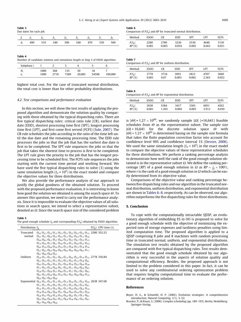
Table 3Due dates for each job.

Ji J1 J2 J3 J4 J5 J6 J7 J8

di 490 510 540 500 540 470 530 560

Table 4Number of candidate solution and simulation length in Step 3 of ESOO algorithm.

Subphase i 1 2 3 4 5 6

Ni 1000 368 135 50 18 7Li 1000 2718 7389 20,085 54598 100,000

Table 6Comparison of F(Sg) and RP for truncated normal distribution.

Method ESOO CR EDD SPT LPT FCFS

F(Sg) 2280 2780 3230 2530 4640 3130RP (%) 0.001 0.003 0.054 0.002 8.663 0.021

Table 7Comparison of F(Sg) and RP for uniform distribution.

Method ESOO CR EDD SPT LPT FCFS

F(Sg) 2778 3734 3093 2823 4707 3660RP (%) 0.001 0.07 0.003 0.002 2.363 0.052

Table 8

S.-C. Horng et al. / Expert Systems with Applications 39 (2012) 3603–3610 3609

highest total cost. For the case of truncated normal distribution,the total cost is lower than for other probability distributions.

Comparison of F(Sg) and RP for exponential distribution.

Method ESOO CR EDD SPT LPT FCFS

F(Sg) 2638 5584 3417 3365 6051 4262RP (%) 0.001 1.203 0.004 0.003 2.912 0.039

4.2. Test comparisons and performance evaluation

In this section, we will show the test results of applying the pro-posed algorithm and demonstrate the solution quality by compar-ing with those obtained by the typical dispatching rules. There arefive typical dispatching rules: critical ratio rule (CR), earliest duedate (EDD), shortest processing time first (SPT), longest processingtime first (LPT), and first come first served (FCFS) (Sule, 2007). TheCR rule schedules the jobs according to the ratio of the time left un-til the due date and the remaining processing time. The EDD ruleprocesses the jobs so that the job that has the earliest due date isfirst to be completed. The SPT rule sequences the jobs so that thejob that takes the shortest time to process is first to be completed.The LPT rule gives the priority to the job that has the longest pro-cessing time to be scheduled first. The FCFS rule sequences the jobsstarting with the current time period and working forward. Wehave used the five typical dispatching rules to solve (3) using thesame simulation length (Le = 105) in the exact model and comparethe objective values for three distributions.

We also provide the performance analysis of our approach tojustify the global goodness of the obtained solution. To proceedwith the proposed performance evaluation, it is interesting to knowhow good the solution we obtained is among the search space H. Toanswer this question, we need to carry out the performance analy-sis. Since it is impossible to evaluate the objective values of all solu-tions in search space, we intend to select a representative subset,denoted as X. Since the search space size of the considered problem

Table 5The good enough schedule Sg and corresponding F(Sg) obtained by ESOO algorithm.

Distribution Sg F(Sg) CPU time (s)

Truncatednormal

O4,2 O2,1 O5,4 O1,3 O5,3 O3,1 O2,2 O5,2 O3,2 O1,2

O4,1 O5,1 O6,3 O2,3 O2,5 O1,1 O4,3 O2,4 O7,1 O5,6

O4,4 O8,2 O8,1 O5,7 O4,6 O3,3 O2,7 O4,7 O5,5 O1,5

O7,4 O2,6 O1,7 O6,1 O5,8 O1,4 O7,2 O2,8 O3,5 O3,4

O4,5 O1,8 O4,8 O3,6 O1,6 O7,3 O3,8 O7,5 O7,8 O7,6

O3,7 O6,2 O8,3 O6,6 O8,4 O6,4 O6,5 O6,8 O8,5 O7,7

O8,7 O8,6 O8,8 O6,7

2280 352.23

Uniform O5,4 O7,1 O3,1 O2,1 O6,3 O1,3 O4,2 O3,2 O7,4 O7,2

O6,1 O5,3 O2,2 O7,3 O2,3 O7,5 O2,5 O1,2 O7,8 O4,1

O4,3 O2,4 O6,2 O3,3 O2,7 O2,6 O7,6 O3,5 O6,6 O2,8

O7,7 O5,2 O3,4 O4,4 O5,1 O3,6 O1,1 O5,6 O6,4 O6,5

O3,8 O3,7 O6,8 O5,7 O4,6 O1,5 O1,7 O5,5 O6,7 O8,2

O8,1 O1,4 O5,8 O8,3 O1,8 O4,7 O4,5 O4,8 O8,4 O1,6

O8,5 O8,7 O8,6 O8,8

2778 356.84

Exponential O6,3 O3,1 O3,2 O1,3 O3,3 O1,2 O5,4 O2,1 O3,5 O3,4

O7,1 O1,1 O7,4 O5,3 O2,2 O1,5 O2,3 O4,2 O2,5 O4,1

O7,2 O7,3 O7,5 O5,2 O6,1 O1,7 O2,4 O4,3 O6,2 O1,4

O7,8 O1,8 O8,2 O6,6 O5,1 O6,4 O4,4 O3,6 O2,7 O2,6

O3,8 O3,7 O2,8 O1,6 O7,6 O5,6 O6,5 O5,7 O7,7 O8,1

O8,3 O4,6 O6,8 O4,7 O5,5 O8,4 O5,8 O8,5 O4,5 O6,7

O8,7 O4,8 O8,6 O8,8

2638 347.68

is |H| = 1.27 � 1089, we randomly sample |X| (=16,641) feasibleschedules from H as the representative subset. The sample size|X| = 16,641 for the discrete solution space H with|H| = 1.27 � 1089 is determined basing on the sample size formulathat takes the finite population correction factor into account forconfidence level 99% and confidence interval 1% (Devore, 2008).We used the same simulation length (Le = 105) in the exact modelto compare the objective values of these representative schedulesfor three distributions. We perform a ranking percentage analysisto demonstrate how well the rank of the good enough solution ob-tained is in the representative subset X. We define the ranking per-centage (RP) of a good enough solution in X as RP ¼ r

jXj � 100%,where r is the rank of a good enough solution in X which can be eas-ily determined from its objective value.

Comparisons of the objective value and ranking percentage be-tween five dispatching rules and our algorithm in the truncated nor-mal distribution, uniform distribution, and exponential distributionare shown in Tables 6–8, respectively. As can be observed, our algo-rithm outperforms the five dispatching rules for three distributions.

5. Conclusion

To cope with the computationally intractable SJSSP, an evolu-tionary algorithm of embedding ES in OO is proposed to solve fora good enough schedule with the objective of minimizing the ex-pected sum of storage expenses and tardiness penalties using lim-ited computation time. The proposed algorithm is applied to aSJSSP comprising 8 jobs and 8 machines with random processingtime in truncated normal, uniform, and exponential distributions.The simulation test results obtained by the proposed algorithmare compared with five typical dispatching rules. Test results dem-onstrated that the good enough schedule obtained by our algo-rithm is very successful in the aspects of solution quality andcomputational efficiency. Besides, the proposed approach is notlimited to the problem considered in this paper. In fact, it can beused to solve any combinatorial ordering optimization problemthat requires lengthy computational time to evaluate the perfor-mance of an ordering solution.

References

Beyer, H. G., & Schwefel, H. P. (2002). Evolution strategies: A comprehensiveintroduction. Natural Computing, 1(1), 3–52.

Brucker, P., & Knust, S. (2006). Complex scheduling (pp. 189–193). Berlin, Heidelberg:Springer-Verlag.

3610 S.-C. Horng et al. / Expert Systems with Applications 39 (2012) 3603–3610

Chakraborty, U. K. (Ed.). (2009). Computational intelligence in flow shop and job shopscheduling. Berlin: Springer.

Devore, J. L. (2008). Probability and statistics for engineering and science (7th ed.). CA:Thomson Brooks/Cole.

Dréo, J., Pétrowski, A., Siarry, P., & Taillard, E. (2006). Metaheuristics for hardoptimization: methods and case studies. Heidelberg, Berlin: Springer-Verlag.

Fattahi, P., Mehrabad, M. S., & Jolai, F. (2007). Mathematical modeling and heuristicapproaches to flexible job shop scheduling problems. Journal of IntelligentManufacturing, 18(3), 331–342.

Gholami, M., & Zandieh, M. (2009). Integrating simulation and genetic algorithm toschedule a dynamic flexible job shop. Journal of Intelligent Manufacturing, 20(4),481–498.

Gu, J. W., Gu, M. Z., Cao, C. W., & Gu, X. S. (2010). A novel competitive co-evolutionary quantum genetic algorithm for stochastic job shop schedulingproblem. Computers and Operations Research, 37(5), 927–937.

Gu, J. W., Gu, X. S., & Gu, M. Z. (2009). A novel parallel quantum genetic algorithmfor stochastic job shop. Journal of Mathematical Analysis and Applications, 355(1),63–81.

Ho, Y. C., Zhao, Q. C., & Jia, Q. S. (2007). Ordinal optimization: Soft optimization forhard problems. New York: Springer-Verlag.

Horng, S. C., & Lin, S. S. (2009). An ordinal optimization theory based algorithm for aclass of simulation optimization problems and application. Expert Systems withApplications, 36(5), 9340–9349.

Keskin, B. B., Melouk, S. H., & Meyer, I. L. (2010). A simulation-optimizationapproach for integrated sourcing and inventory decisions. Computers andOperations Research, 37(9), 1648–1661.

Lei, D. M. (2010). A genetic algorithm for flexible job shop scheduling with fuzzyprocessing time. International Journal of Production Economics, 48(10), 2995–3013.

Li, J., Sava, A., & Xie, X. L. (2009). Simulation-based discrete optimization ofstochastic discrete event systems subject to non closed-form constraints. IEEETransactions on Automatic Control, 54(12), 2900–2904.

Mezura-Montes, E., & Coello, C. A. C. (2008). An empirical study about theusefulness of evolution strategies to solve constrained optimization problems.International Journal of General Systems, 37(4), 443–473.

Renna, P. (2010). Job shop scheduling by pheromone approach in a dynamicenvironment. International Journal of Computer Integrated Manufacturing, 23(5),412–424.

Shen, Z., Ho, Y. C., & Zhao, Q. C. (2009). Ordinal optimization and quantification ofheuristic designs. Discrete Event Dynamic Systems, 19(3), 317–345.

Sule, D. R. (2007). Production planning and industrial scheduling: Examples case studiesand applications (2nd ed.). Boston: PWS Publishing.

Tavakkoli-Moghaddam, R., Jolai, F., Vaziri, F., Ahmed, P. K., & Azaron, A. (2005). Ahybrid method for solving stochastic job shop scheduling problems. AppliedMathematics and Computation, 170(1), 185–206.

Zandieh, M., & Adibi, M. A. (2010). Dynamic job shop scheduling using variableneighbourhood search. International Journal of Production Research, 48(8),2449–2458.

Zhang, R., & Wu, C. (2010). A hybrid approach to large-scale job shop scheduling.Applied Intelligence, 32(1), 47–59.

Zhou, R., Nee, A. Y. C., & Lee, H. P. (2009). Performance of an ant colony optimisationalgorithm in dynamic job shop scheduling problems. International Journal oProduction Research, 47(11), 2903–2920.