Single machine stochastic appointment sequencing and scheduling

We develop algorithms for a single machine stochastic appointment sequencing and scheduling problem

with waiting time, idle time, and overtime costs. This is a basic stochastic scheduling problem that has

been studied in various forms by several previous authors. Applications for this problem cited previously

include scheduling of surgeries in an operating room (Denton, 2007, Denton and Gupta,2003), scheduling

of appointments in a clinic (Robinson and Chen, 2003, Vanden Bosch, 2000), (Wang, 1997) mentions the

application of this problem to scheduling of ships in a port. Begen and Queyranne (2009) discuss this

problem in the context of scheduling exams in an examination facility (MRI, Scans). In this paper the

problem is formulated as a stochastic integer program using sample average approximation. A heuristic

solution approach based on Benders' decomposition is developed and compared to exact methods and to

previously proposed approaches. Extensive computational testing shows that the proposed methods

produce good results compared to previous approaches. In addition we prove that the finite scenario

sample average approximation problem is NP-complete.

1. Introduction

The problem we address assumes a finite set of jobs with stochastic processing times. It is assumed that

the processing time duration of the jobs are random variables with known joint distribution. The marginal

distributions of job durations are not assumed identical. The problem requires us to find the sequence in

which to perform the jobs, and to assign a starting time to each job. A job may not begin before its

scheduled starting time nor may it begin until the previous job is complete. If the ith job in the sequence

finishes before the i+1st job is scheduled to start, then there will be idle time on the machine. Conversely,

if the ith job in the sequence finishes after the i+1

st job is scheduled to start, then job i+1 will incur waiting

time. Further, if the last job finishes after a predefined deadline, there will be overtime. The objective is

to determine the sequence and scheduled starting times of jobs on the machine that minimize a weighted

linear combination of job waiting time, machine idle time, and overtime. We assume a separate cost (per

unit time) for each job for both waiting and idle times, and a single overtime cost. Since we explicitly

consider the randomness of the job processing times, the objective is to minimize total expected cost

where expectation is taken with respect to the joint distribution of surgery times.

This problem has been called the “appointment scheduling problem” because it is easy to envision by

analogy to scheduling appointments in a physician’s office. Jobs represent patient appointments, while

the doctor represents the machine. Waiting time is the time patients must wait beyond their scheduled

appointment time while idle time represents time the doctor is not busy while waiting for the next patient

to arrive.

The problem can be decomposed into two parts. The first is to determine the sequence in which the jobs

will be performed. Given a sequence one must next determine the amount of time to allocate to each job,

or equivalently assign each job a scheduled starting time. This second problem (which we call the

scheduling problem) has been studied previously under the name “stochastic appointment scheduling”.

Previous approaches to this problem include using convolutions to compute starting times (Weiss, 1990),

sample average approximation and the L-Shape Algorithm (Denton, 2003), and heuristics (Robinson and

Chen, 2003). We will approach this problem using sample average approximation and linear

programming in a similar fashion to (Denton, 2007).

Given reasonably efficient methods to solve the scheduling problem, we next develop an algorithm for the

sequencing problem. According to (Gupta, 2007) the sequencing problem is still an open question. The

main idea of the proposed method is based on a Benders' decomposition scheme. The master problem is

used to find sequences and the sub-problems are the scheduling problems (stochastic linear programs)

as discussed above. The Benders' master problem becomes extremely hard to solve as cuts are added,

thus we turn to heuristics to approximate its solution and generate promising sequences.

The remainder of the article is organized as follows. In the next section a brief review of the literature

related to the sequencing and scheduling problems and stochastic integer programming is provided. In

Section 3, the model is described and formulated. In Section 4 new complexity results for the sequencing

problem are presented. In Section 5 algorithms are proposed to solve the sequencing and scheduling

problems. In Section 6 a method is proposed to choose the number of scenarios. In Section 7

computational results are presented. In Section 8 conclusions and future research directions are

discussed.

2. Literature Review

Relevant previous work can be divided in two categories: stochastic appointment scheduling and

stochastic integer programming. We begin with previous work on the stochastic appointment scheduling

problem. (Weiss, 1990) found the optimal sequence when there are only 2 jobs (i.e. convex order) and

then showed that this criterion does not guarantee optimality when the number of jobs is greater than 2.

(Wang, 1997) assumed job durations were i.i.d. random variables following a Coxian (phase type)

distribution. Since durations were i.i.d., sequencing was irrelevant. He assumed costs for waiting time

and total completion time. He developed an efficient numerical procedure to calculate mean job flow

times then solved for the optimal scheduled starting times using non-linear programming. For examples

with up to 10 jobs, he showed that even though job durations are i.i.d., the optimal starting times are not

equally spaced.

(Denton, 2007) formulated the sequencing and scheduling problem as an stochastic integer program and

then proposed simple heuristics to determine the sequence. Once a sequence is given, the schedule of

starting times was found using a sample average approximation (i.e. scenario based) approach. The

resulting scheduling problem was shown to be a linear stochastic program which they solved by an L-

shaped algorithm described in (Denton, 2003). To determine a sequence they proposed three methods:

sort by variance of duration, sort by mean of duration, and sort by coefficient of variation of duration.

These simple heuristics were also compared to a simple interchange heuristic. The application studied in

in (Denton, 2003) was scheduling surgeries in a single operating room. They reported results with real

surgery time data and up to 12 surgeries (jobs). They also assumed equal penalty costs across surgeries

for waiting and idle time. They found that sort by variance of duration gave the best results.

(Kaandorp and Koole, 2007) assumed that job durations were Exponentially distributed with different

means and that patient arrivals can only be scheduled at finite times (every ten minutes). Their objective

function included waiting time, idle time, and overtime costs. Given these assumptions, a queuing theory

approach was used to calculate the objective function for a given schedule of starting times. They further

proved that the objective function was multi-modular with respect to a neighborhood that can move the

start time of jobs one interval earlier or later. This result guaranteed that a local search algorithm in this

neighborhood will find the optimal solution. In (Kong, 2010) the authors developed a robust optimization

approach to the appointment scheduling problem. They assumed that the distributions of the services

was unknown, and minimized the worst case expected value over a family of distributions to determine

the schedule. In (Vanden Bosch, 2000) and (Vanden Bosch, 2001) the authors also assumed discrete scheduled

starting times (at 10 minute intervals over 3 hours) and included penalties for waiting time and overtime.

They assumed three classes of patients in an outpatient appointment scheduling setting where durations

were i.i.d. within class but different between classes. They used Phase Type and Lognormal distributions

to model the three duration distributions. Given a sequence, they proposed a gradient based algorithm to

find the optimal schedule of starting times based on submodularity properties of the objective function.

They proposed an all-pairs swap-based steepest decent local search heuristic to find a sequence. They

stopped the search after a fixed number of iterations or when a local minimum is found. They reported

testing with simulated data for cases with 4 and 6 jobs and concluded that the heuristics produced good

results in terms of iterations and optimality gap when compared with exhaustive enumeration.

The approach to the problem taken in this paper is stochastic integer programming, thus previous

approaches to similar problems are relevant. There is a rich literature on stochastic integer programming.

In (Schulz, 2003) a thorough review of methods for solving stochastic programming problems with integer

variables was given. For the type of problem we address, there are several methods that might seem to

apply. Our problem has both integer variables (for sequencing) and continuous variables (for scheduled

starting times) in the first stage, continuous variables in the recourse function (waiting and idle times), and

complete recourse. For finite scenario problems, (Laporte, 1993) proposed the Integer L-Shaped Method,

an algorithm that is suitable for solving Stochastic Programs where the first stage variables are binary and

the recourse cost is easily computable. The method uses Benders' Decomposition combined with cuts

that differ from traditional Benders' cuts. Another approach based on scenario decomposition was

proposed in (Caroe, 1997). After decomposing the problem by scenarios, they then solved a problem

with relaxed non-anticipativity constraints to get a lower bound within a branch and bound scheme. Finally

there is the widely used Benders' decomposition approach. In Benders' approach one may decompose

by fixing the integer variables or by fixing the set of all first stage decisions. The problem we address is

such that if the integer (sequencing) variables are fixed, the continuous (scheduling) variables can be

computed with relative ease by solving a linear program using an interior point method. This makes

Benders' decomposition particularly attractive for our problem. We also experimented briefly with the

Integer L-shaped method but found that it offered no advantage over the Benders' approach in this case.

Scenario decomposition is not appropriate for our problem since solutions to the single scenario problems

provide no useful information about the overall solution. This is because in any scenario subproblem, the

starting times are simply set equal to the finish time of the previous job always resulting in zero cost.

The current literature also distinguishes between infinite scenario problems and finite scenario problems.

For the infinite scenario case, two methodologies are potentially useful. In (Homen de Mello, 2002) the

authors proposed an algorithm for solving the sample average approximation (finite scenario problem).

They applied this procedure many times until stopping criteria related to statistical bounds are fulfilled.

The other method aimed at the infinite scenario case is Stochastic Branch and Bound (Ruszczynski,

1998). This method partitions the integer feasible space and computes statistical upper and lower

bounds, then uses these bounds in the same way traditional branch and bound uses upper and lower

bounds to find the true optimal value with probability one. Solving our sample average approximation

problem turns out to be very time consuming, thus neither of these infinite scenario approaches are

practically viable in our case.

3. Problem Statement

We assume a finite set of jobs with durations that are random variables. We assume these job durations

have a known joint distribution, and are independent of the position in the sequence to which the job is

assigned. Only one job may be performed at a time, and overtime is incurred when job processing

extends past a deadline representing the length of the work day. Two sets of decisions must be made,

first the job sequence must be determined, then a starting time must be assigned to each job. In

application to surgery scheduling, the starting time can be thought of as the time the patient is scheduled

to arrive thus a job (surgery) may not begin before its scheduled starting time. The objective function

consists of three components, waiting time (the time a patient must wait between his/her scheduled

starting time and actual starting time), idle time (the time the O.R. is idle while waiting for the next patient

to arrive) and overtime. Given a sequence, starting times for each job, and the duration distributions, the

expected waiting time and idle time before each job and the over time can be estimated by averaging

over a sample of scenarios. The objective function is a weighted linear combination of these three

expected costs. Note that waiting and idle costs may be different for each job.

This problem has been modeled as a two stage stochastic program with binary and continuous variables

in the first stage decisions in (Denton, 2007). They incorporated the processing time uncertainty into the

model using a sample average approximation (i.e. scenario based) approach. The binary variables

define which job (surgery) should be placed in the ith position in the sequence. The starting times and the

binary variables are all included in the first stage decisions. This problem can be formulated as shown

below. This model is similar to (Denton, 2007).

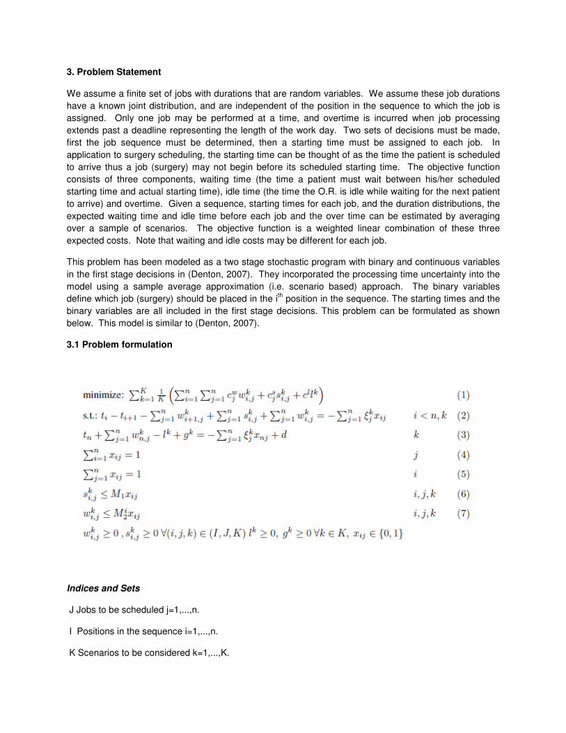
3.1 Problem formulation

Indices and Sets

J Jobs to be scheduled j=1,...,n.

I Positions in the sequence i=1,...,n.

K Scenarios to be considered k=1,...,K.

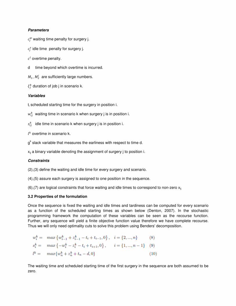
Parameters

��� waiting time penalty for surgery j.

��� idle time penalty for surgery j.

�� overtime penalty.

d time beyond which overtime is incurred.

��, � are sufficiently large numbers.

��� duration of job j in scenario k.

Variables

ti scheduled starting time for the surgery in position i.

�� waiting time in scenario k when surgery j is in position i.

��� idle time in scenario k when surgery j is in position i.

�� overtime in scenario k.

gk slack variable that measures the earliness with respect to time d.

xij a binary variable denoting the assignment of surgery j to position i.

Constraints

(2),(3) define the waiting and idle time for every surgery and scenario.

(4),(5) assure each surgery is assigned to one position in the sequence.

(6),(7) are logical constraints that force waiting and idle times to correspond to non-zero xij

3.2 Properties of the formulation

Once the sequence is fixed the waiting and idle times and tardiness can be computed for every scenario

as a function of the scheduled starting times as shown below (Denton, 2007). In the stochastic

programming framework the computation of these variables can be seen as the recourse function.

Further, any sequence will yield a finite objective function value therefore we have complete recourse.

Thus we will only need optimality cuts to solve this problem using Benders' decomposition.

The waiting time and scheduled starting time of the first surgery in the sequence are both assumed to be

zero.

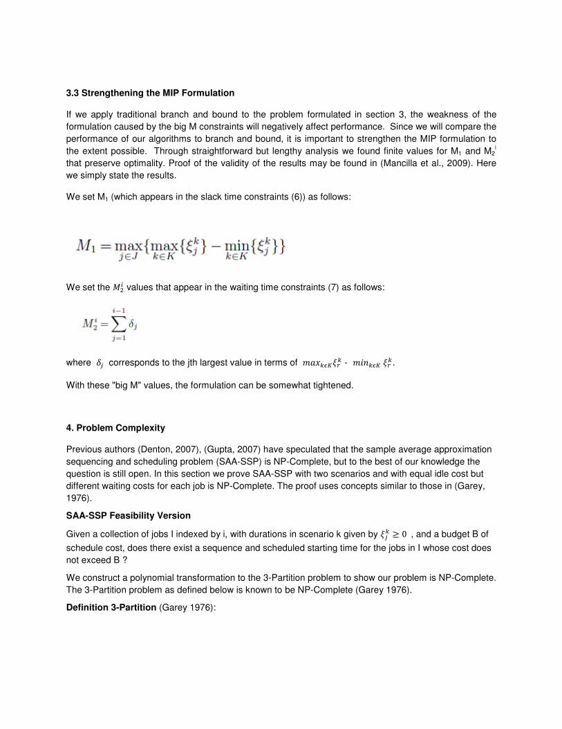
3.3 Strengthening the MIP Formulation

If we apply traditional branch and bound to the problem formulated in section 3, the weakness of the

formulation caused by the big M constraints will negatively affect performance. Since we will compare the

performance of our algorithms to branch and bound, it is important to strengthen the MIP formulation to

the extent possible. Through straightforward but lengthy analysis we found finite values for M1 and M2i

that preserve optimality. Proof of the validity of the results may be found in (Mancilla et al., 2009). Here

we simply state the results.

We set M1 (which appears in the slack time constraints (6)) as follows:

We set the � values that appear in the waiting time constraints (7) as follows:

where �� corresponds to the jth largest value in terms of ��������� - ������ ��

�.

With these "big M" values, the formulation can be somewhat tightened.

4. Problem Complexity

Previous authors (Denton, 2007), (Gupta, 2007) have speculated that the sample average approximation

sequencing and scheduling problem (SAA-SSP) is NP-Complete, but to the best of our knowledge the

question is still open. In this section we prove SAA-SSP with two scenarios and with equal idle cost but

different waiting costs for each job is NP-Complete. The proof uses concepts similar to those in (Garey,

1976).

SAA-SSP Feasibility Version

Given a collection of jobs I indexed by i, with durations in scenario k given by ��� � 0 , and a budget B of

schedule cost, does there exist a sequence and scheduled starting time for the jobs in I whose cost does

not exceed B ?

We construct a polynomial transformation to the 3-Partition problem to show our problem is NP-Complete.

The 3-Partition problem as defined below is known to be NP-Complete (Garey 1976).

Definition 3-Partition (Garey 1976):

Given positive integers n, R, and a set of integers A = {a1, a2,...,a3n} with nRan

ii =∑

=

3

1

and 24

Ra

Ri << for

1 ≤ i ≤ 3n, does there exist a partition < A1, A2,. ,....An > of A into 3-elements sets such that, for each

p=1,…,n RapAa

=∑∈

?

Theorem 1

The Sample Average Approximation Sequencing and Scheduling Problem (SAA-SSP) with two scenarios

is NP-Complete when the waiting costs are allowed to differ between jobs.

Construction

We show that 3-partition polynomially reduces to a particular SAA-SSP with 2 scenarios. We construct an

instance of SAA-SSP with 4n jobs and 2 scenarios in which the first 3n jobs (job set “G” indexed by

i=1,…,3n) have durations ii a=1ξ and nifori 3102 ≤≤=ξ . The remaining n jobs (job set “V” indexed

by i=3n+1, …, 4n) have durations Hi =1ξ , and RHi +=2ξ for nin 413 ≤≤+ . ( H is an integer

number) The idle cost penalties are chosen as KRncs

i

210= for all 4n jobs. The waiting cost for jobs in

V are nnifornR

cwi 4,...,13

2

5+== and for jobs in set G: 1=w

ic for ni 3,...,1= . The budget of the

schedule cost is 4

5nRB = .

Intuitively, the main idea of the proof can be seen in Figure 1. The schedule consists of n blocks with

each block containing one of the partitions in scenario 1. The idle cost is set high enough to guarantee

that there will be no idle time in an optimal solution to the SAA-SSP. The scheduled starting time for

every job is set equal to its actual starting time in scenario 1. We first show that if a 3-partition exists, the

schedule below will meet the budget B. We then show that if the schedule is not the "3-Partition

schedule" as shown in Figure 1, or if no partition exists, then the budget to be exceeded.

Figure 1: 2 Scenario Case: (ap,1 means partition p the first element)

Scenario 1

Scenario 2

Zero processing time G jobs

H

R

a1,1 a1,2 a1,3

H+R

Block 1

H

R

a2,1 a2,2 a2,3

H+R

Block 2

Zero processing time G jobs

Scheduled starting times Scheduled starting times

Scenario 1

Scenario 2

Zero processing time G jobs

H

R

a1,1 a1,2 a1,3

H+R

Block 1

H

R

a2,1 a2,2 a2,3

H+R

Block 2

Zero processing time G jobs

Scheduled starting times Scheduled starting times

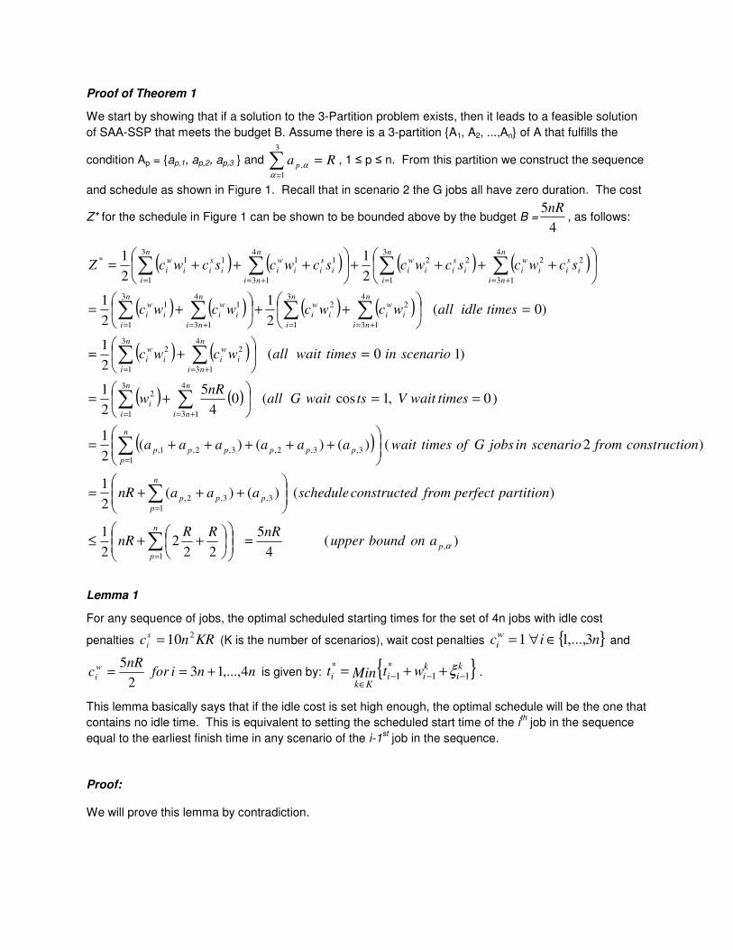
Proof of Theorem 1

We start by showing that if a solution to the 3-Partition problem exists, then it leads to a feasible solution

of SAA-SSP that meets the budget B. Assume there is a 3-partition {A1, A2, ...,An} of A that fulfills the

condition Ap = {ap,1, ap,2, ap,3 } and Ra p =∑=

3

1

,

αα , 1 ≤ p ≤ n. From this partition we construct the sequence

and schedule as shown in Figure 1. Recall that in scenario 2 the G jobs all have zero duration. The cost

Z* for the schedule in Figure 1 can be shown to be bounded above by the budget B =4

5nR, as follows:

( ) ( ) ( ) ( )

( ) ( ) ( ) ( )

( ) ( )

( ) ( )

( )

)(4

5

222

2

1

)()()(2

1

)2()()()(2

1

)0,1cos(04

5

2

1

)10(2

1

)0(2

1

2

1

2

1

2

1

,

1

1

3,3,2,

1

3,3,2,3,2,1,

3

1

4

13

2

3

1

4

13

22

3

1

4

13

223

1

4

13

11

3

1

4

13

22223

1

4

13

1111*

αp

n

p

n

p

ppp

n

p

pppppp

n

i

n

ni

i

n

i

n

ni

i

w

ii

w

i

n

i

n

ni

i

w

ii

w

i

n

i

n

ni

i

w

ii

w

i

n

i

n

ni

i

s

ii

w

ii

s

ii

w

i

n

i

n

ni

i

s

ii

w

ii

s

ii

w

i

aonbounduppernRRR

nR

partitionperfectfromdconstructescheduleaaanR

onconstructifromscenarioinjobsGoftimeswaitaaaaaa

timeswaitVtswaitGallnR

w

scenariointimeswaitallwcwc

timesidleallwcwcwcwc

scwcscwcscwcscwcZ

=

++≤

+++=

+++++=

==

+=

=

+=

=

++

+=

++++

+++=

∑

∑

∑

∑ ∑

∑ ∑

∑ ∑∑ ∑

∑ ∑∑ ∑

=

=

=

= +=

= +=

= +== +=

= +== +=

Lemma 1

For any sequence of jobs, the optimal scheduled starting times for the set of 4n jobs with idle cost

penalties KRncs

i

210= (K is the number of scenarios), wait cost penalties { }nic

wi 3,...,11 ∈∀= and

nnifornR

cw

i 4,...,132

5+== is given by: { }k

ikii

Kki wtMint 11

*1

*−−−

∈++= ξ .

This lemma basically says that if the idle cost is set high enough, the optimal schedule will be the one that

contains no idle time. This is equivalent to setting the scheduled start time of the ith job in the sequence

equal to the earliest finish time in any scenario of the i-1st job in the sequence.

Proof:

We will prove this lemma by contradiction.

Case 1: Assume that ∃ a job i such that { }ki

kii

Kki wtMint 11

*1

*−−−

∈++< ξ in the optimal schedule. This means

that job i has positive waiting time in every scenario (i.e. Kkwki ∈∀> 0 ). This contradicts the assumed

fact that this is an optimal solution since we can increase *it until some

kiw becomes zero without

affecting the waiting time of the other jobs. This implies that we were in a suboptimal solution.

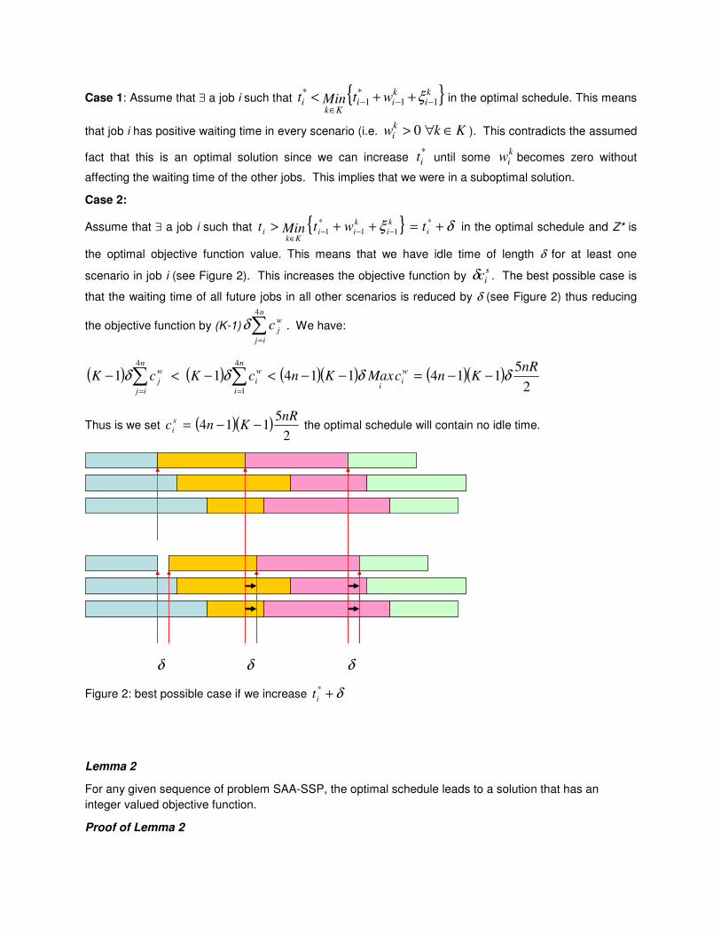
Case 2:

Assume that ∃ a job i such that { } δξ +=++> −−−∈

*

11

*

1 i

k

i

k

iiKk

i twtMint in the optimal schedule and Z* is

the optimal objective function value. This means that we have idle time of length δ for at least one

scenario in job i (see Figure 2). This increases the objective function by sicδ . The best possible case is

that the waiting time of all future jobs in all other scenarios is reduced by δ (see Figure 2) thus reducing

the objective function by (K-1) ∑=

n

ij

w

jc4

δ . We have:

( ) ( ) ( )( ) ( )( )2

511411411

4

1

4 nRKncMaxKncKcK

w

ii

n

i

w

i

n

ij

w

j δδδδ −−=−−<−<− ∑∑==

Thus is we set ( )( )2

5114

nRKnc

s

i −−= the optimal schedule will contain no idle time.

--------------------------------------------------------

δ δ δ

Figure 2: best possible case if we increase δ+*

it

Lemma 2

For any given sequence of problem SAA-SSP, the optimal schedule leads to a solution that has an

integer valued objective function.

Proof of Lemma 2

By lemma 1 we know that the scheduled starting times follow a recursive formula that depends on waiting

time and durations of jobs earlier in the sequence: { }ki

kii

Kki wtMintt 11

*1

**1 ,0 −−−

∈++== ξ Further we

know that we can express waiting time of the ith job in the sequence using:

i

i

j

kj

ki

k tww −∑==−

=

1

11 ,0 ξ . Since the durations are integers, and the integers are closed under addition

and subtraction, we can conclude that all waiting times are integer (and all idle times are zero). Since

waiting costs are also integer, the objective function value of the optimal solution to the scheduling

problem is an integer.

Lemma 3

The actual starting times of jobs in set V must be the same in each scenario otherwise the budget will be

exceeded.

Proof of Lemma 3

Since no idle time can exist (Lemma 1), the schedule for scenario 2 must appear as below. If the V jobs

in scenario 1 do not start at the same time as in scenario 2, there will be non-zero waiting time for at least

1 V job. The waiting time must be at least 1 (from the integer lemma 2), and since waiting cost for jobs in

V is 5nR/2, the budget is exceeded

Thus the schedule for V jobs must look like this

Figure 3: Optimal sequencing pattern.

Lemma 4

There must be subsets of G jobs that fit perfectly into the first n-1 open slots (of width R) in the schedule

above if there exists a perfect partition. These subsets consist of 3 G jobs and correspond to the perfect

partition.

Proof of Lemma 4

If do not exist these subsets of G jobs there will be idle time in the schedule, and the budget will be

exceeded (by Lemma 1). Therefore these subsets must consist of 3 G jobs due to the

bounds24

Ra

Ri << , otherwise the subsets will add to more or less than R. The only possible solution for

these subsets is the perfect partition and by definition of the partition problem, the remaining 3 jobs must

fit perfectly into the last open slot.

With Lemma 4 we can conclude that the SAA-SSP with two scenarios is NP-complete when the waiting

costs are allowed to differ between jobs.

H

R

H+R

Scenario 1

Scenario 2

H

R

H+R

H

R

H+R

H

R

H+R

Scenario 1

Scenario 2

H

R

H+R

H

R

H+R

5. Proposed Solution Methodology

The approach we propose for the SAA-SSP uses a heuristic method to find good solutions in a

reasonable amount of time. The Master problem in our Benders' Decomposition is an integer program,

and thus is difficult to solve and even more difficult as we add more cuts in every iteration. Relaxing the

side constraints (optimality Benders’ cuts) results in an easy to solve assignment problem. We use this

property to construct a heuristic to generate good feasible solutions to the master problem. The idea of

solving the master problem heuristically has also been proposed by several authors including (Cote,

1984) and (Aardal, 1990).

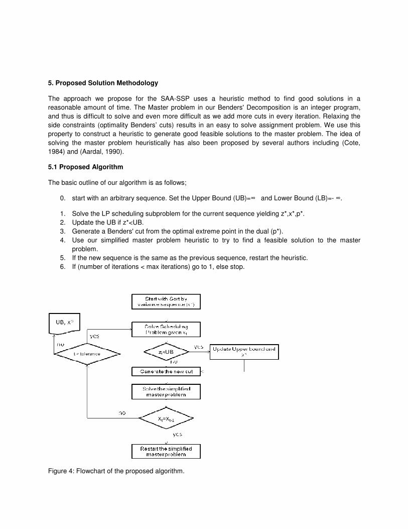
5.1 Proposed Algorithm

The basic outline of our algorithm is as follows;

0. start with an arbitrary sequence. Set the Upper Bound (UB)=∞ and Lower Bound (LB)=- ∞.

1. Solve the LP scheduling subproblem for the current sequence yielding z*,x*,p*.

2. Update the UB if z*<UB.

3. Generate a Benders' cut from the optimal extreme point in the dual (p*).

4. Use our simplified master problem heuristic to try to find a feasible solution to the master

problem.

5. If the new sequence is the same as the previous sequence, restart the heuristic.

6. If (number of iterations < max iterations) go to 1, else stop.

Figure 4: Flowchart of the proposed algorithm.

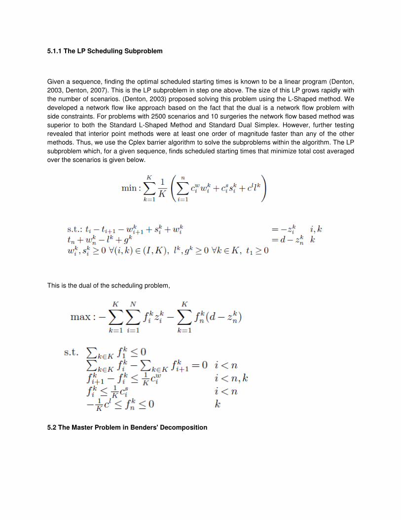
5.1.1 The LP Scheduling Subproblem

Given a sequence, finding the optimal scheduled starting times is known to be a linear program (Denton,

2003, Denton, 2007). This is the LP subproblem in step one above. The size of this LP grows rapidly with

the number of scenarios. (Denton, 2003) proposed solving this problem using the L-Shaped method. We

developed a network flow like approach based on the fact that the dual is a network flow problem with

side constraints. For problems with 2500 scenarios and 10 surgeries the network flow based method was

superior to both the Standard L-Shaped Method and Standard Dual Simplex. However, further testing

revealed that interior point methods were at least one order of magnitude faster than any of the other

methods. Thus, we use the Cplex barrier algorithm to solve the subproblems within the algorithm. The LP

subproblem which, for a given sequence, finds scheduled starting times that minimize total cost averaged

over the scenarios is given below.

This is the dual of the scheduling problem,

5.2 The Master Problem in Benders' Decomposition

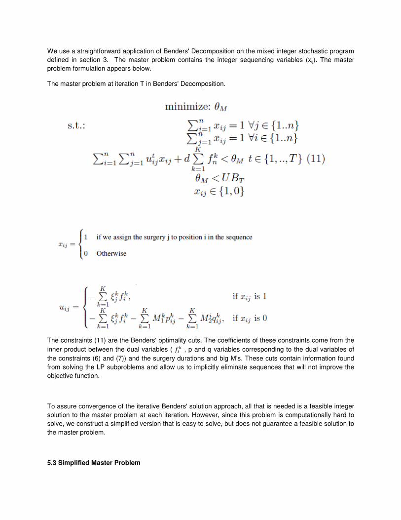
We use a straightforward application of Benders' Decomposition on the mixed integer stochastic program

defined in section 3. The master problem contains the integer sequencing variables (xij). The master

problem formulation appears below.

The master problem at iteration T in Benders' Decomposition.

The constraints (11) are the Benders' optimality cuts. The coefficients of these constraints come from the

inner product between the dual variables ( �� , p and q variables corresponding to the dual variables of

the constraints (6) and (7)) and the surgery durations and big M’s. These cuts contain information found

from solving the LP subproblems and allow us to implicitly eliminate sequences that will not improve the

objective function.

To assure convergence of the iterative Benders' solution approach, all that is needed is a feasible integer

solution to the master problem at each iteration. However, since this problem is computationally hard to

solve, we construct a simplified version that is easy to solve, but does not guarantee a feasible solution to

the master problem.

5.3 Simplified Master Problem

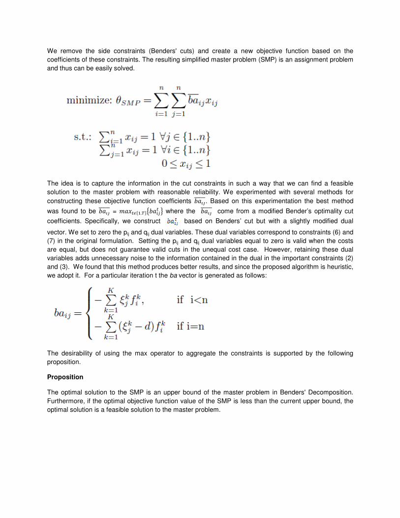
We remove the side constraints (Benders' cuts) and create a new objective function based on the

coefficients of these constraints. The resulting simplified master problem (SMP) is an assignment problem

and thus can be easily solved.

The idea is to capture the information in the cut constraints in such a way that we can find a feasible

solution to the master problem with reasonable reliability. We experimented with several methods for

constructing these objective function coefficients ���������. Based on this experimentation the best method

was found to be ��������� = ��� �!�.#$%���

& where the ��������� come from a modified Bender’s optimality cut

coefficients. Specifically, we construct based on Benders’ cut but with a slightly modified dual

vector. We set to zero the pij and qij dual variables. These dual variables correspond to constraints (6) and

(7) in the original formulation. Setting the pij and qij dual variables equal to zero is valid when the costs

are equal, but does not guarantee valid cuts in the unequal cost case. However, retaining these dual

variables adds unnecessary noise to the information contained in the dual in the important constraints (2)

and (3). We found that this method produces better results, and since the proposed algorithm is heuristic,

we adopt it. For a particular iteration t the ba vector is generated as follows:

The desirability of using the max operator to aggregate the constraints is supported by the following

proposition.

Proposition

The optimal solution to the SMP is an upper bound of the master problem in Benders' Decomposition.

Furthermore, if the optimal objective function value of the SMP is less than the current upper bound, the

optimal solution is a feasible solution to the master problem.

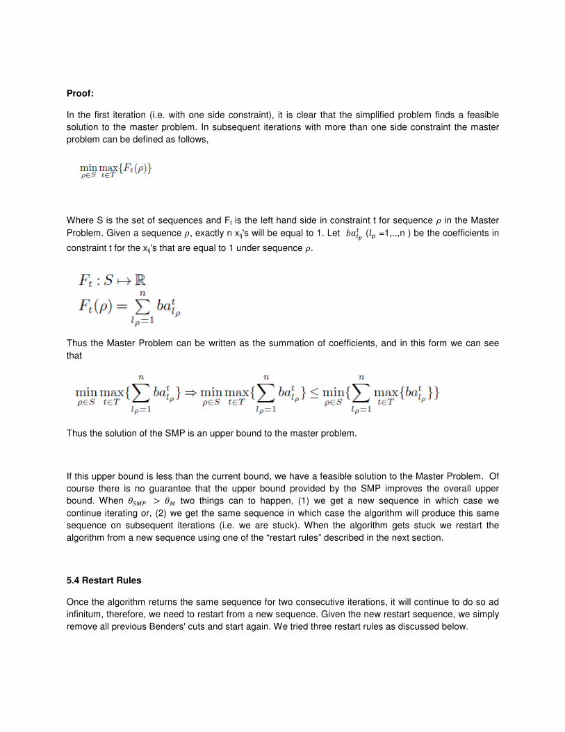
Proof:

In the first iteration (i.e. with one side constraint), it is clear that the simplified problem finds a feasible

solution to the master problem. In subsequent iterations with more than one side constraint the master

problem can be defined as follows,

Where S is the set of sequences and Ft is the left hand side in constraint t for sequence ' in the Master

Problem. Given a sequence ', exactly n xij's will be equal to 1. Let ���( (�) =1,..,n ) be the coefficients in

constraint t for the xij's that are equal to 1 under sequence '.

Thus the Master Problem can be written as the summation of coefficients, and in this form we can see

that

Thus the solution of the SMP is an upper bound to the master problem.

If this upper bound is less than the current bound, we have a feasible solution to the Master Problem. Of

course there is no guarantee that the upper bound provided by the SMP improves the overall upper

bound. When *+,- . *, two things can to happen, (1) we get a new sequence in which case we

continue iterating or, (2) we get the same sequence in which case the algorithm will produce this same

sequence on subsequent iterations (i.e. we are stuck). When the algorithm gets stuck we restart the

algorithm from a new sequence using one of the “restart rules” described in the next section.

5.4 Restart Rules

Once the algorithm returns the same sequence for two consecutive iterations, it will continue to do so ad

infinitum, therefore, we need to restart from a new sequence. Given the new restart sequence, we simply

remove all previous Benders' cuts and start again. We tried three restart rules as discussed below.

5.4.1 Worst Case

This anti-cycling rule is based on finding a sequence "far way" from sequences visited since the last

restart. To accomplish this we simple replace "minimize" with "maximize" in the SMP objective function.

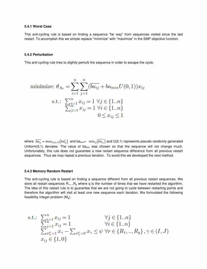
5.4.2 Perturbation

This anti-cycling rule tries to slightly perturb the sequence in order to escape the cycle.

where ��������� = ��� �!�.#$%���

& and bamin= ����%����������& and U(0,1) represents pseudo-randomly generated

Uniform(0,1) deviates. The value of bamin was chosen so that the sequence will not change much.

Unfortunately, this rule does not guarantee a new restart sequence difference from all previous restart

sequences. Thus we may repeat a previous iteration. To avoid this we developed the next method.

5.4.3 Memory Random Restart

This anti-cycling rule is based on finding a sequence different from all previous restart sequences. We

store all restart sequences R1,..,Rq where q is the number of times that we have restarted the algorithm.

The idea of this restart rule is to guarantee that we are not going to cycle between restarting points and

therefore the algorithm will visit at least one new sequence each iteration. We formulated the following

feasibility integer problem (Mq).

Where / is random number generated from IntUniform(0,n-1). We use Cplex to find a feasible solution.

Cplex finds a feasible solution extremely quickly as it turns out, so that the impact on the algorithm's

execution time is minimal. The constraints that contain the previous restart points guarantee that we will

not restart the next iteration from these previous sequences. Further, the random number / serves as a

kind of distance from the set of restarting points where when / =n-1 we might obtain a feasible sequence

for Mq that differs from restart sequences Rr in at most 2 elements. When / =0 the new restart sequence

will differ from every previous restart point in all the elements.

6. Accuracy of the Finite Sample Average Approximation

The ultimate goal is to solve the infinite scenario stochastic programming problem. The method proposed

in this research attempts to solve a finite scenario problem. Further, the method does not guarantee an

optimal solution to this finite scenario problem. In this section we will try to evaluate how our algorithm

will perform on the infinite scenario problem. (Linderoth, 2002) developed a way to compute statistical

upper and lower bounds on the optimal solution to the infinite scenario case based on external sampling

techniques. Unfortunately, this method requires solving a finite scenario problem many many times and

thus is computational prohibitive in our case, even for a small number of scenarios. We therefore

designed a simpler experiment to quantify the performance of our algorithm on the infinite scenario case.

There are two main issues. The first issue is sampling error, that is: "How well is the infinite scenario

objective function approximated by the finite scenario (sample average) objective function?" The second

issue is: "How does the run time of the algorithm affect performance with respect to the infinite scenario

problem?" There is a basic tradeoff we need to evaluate. For a fixed computation time allowance, how

many scenarios should we use? If we use many scenarios, we will only have time to generate a few

candidate sequences thus limiting our ability to "optimize". On the other hand with few scenarios, we can

generate many sequences, and perhaps even solve the finite scenario problem to optimality. However,

the optimal solution to the finite scenario problem may be a poor solution to the infinite scenario problem

when the number of scenarios is small. To quantify this tradeoff we constructed the following experiment.

We generated 50 test problems with 10 jobs each. For each of these 50 problems we generated finite

scenario instances with 50, 100, 250, and 500 scenarios. For each of these 200 instances we then ran

the algorithm for 20,40,60,80,100,120,140 seconds (the experiments were conducted under the same

computational conditions detailed in section 7). For each run of the algorithm we saved the best ten

sequences where "best" is with respect to the number of scenarios used in the current run. This resulted

in the generation of 7x4x10=280 (not necessarily all different) total sequences for each of the 50 test

problems. For each of these sequences, we solved the LP scheduling sub-problem with 10,000

scenarios and reported the best sequence S*10000 and objective function z*10000 found. This serves as our

approximation to an overall best solution to the infinite scenario problem for each of the 50 test cases.

Our first set of results is aimed at understanding the sampling error. The basic question we asked is:

"How often does the sequence our algorithm thinks is best turn out to be the best sequence in the 10,000

scenario case?". For each of the "10 best" sequences returned by the algorithm after 140 seconds of

running, the plots below show the cumulative frequency for which that solution was best for 10,000

scenarios. For example Figure 5 shows that for 500 scenarios, the solution judged to be the best of the

top ten by the algorithm was indeed the best of the top ten 40% of the time. By examining the plot we

see that 50 and 100 scenarios incur significant sampling error since each of the top ten solutions has

essentially the same probability of being best for the 10,000 scenario case. With 500 scenarios, we see

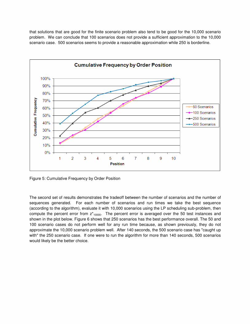
that solutions that are good for the finite scenario problem also tend to be good for the 10,000 scenario

problem. We can conclude that 100 scenarios does not provide a sufficient approximation to the 10,000

scenario case. 500 scenarios seems to provide a reasonable approximation while 250 is borderline.

Figure 5: Cumulative Frequency by Order Position

The second set of results demonstrates the tradeoff between the number of scenarios and the number of

sequences generated. For each number of scenarios and run times we take the best sequence

(according to the algorithm), evaluate it with 10,000 scenarios using the LP scheduling sub-problem, then

compute the percent error from z*10000. The percent error is averaged over the 50 test instances and

shown in the plot below. Figure 6 shows that 250 scenarios has the best performance overall. The 50 and

100 scenario cases do not perform well for any run time because, as shown previously, they do not

approximate the 10,000 scenario problem well. After 140 seconds, the 500 scenario case has "caught up

with" the 250 scenario case. If one were to run the algorithm for more than 140 seconds, 500 scenarios

would likely be the better choice.

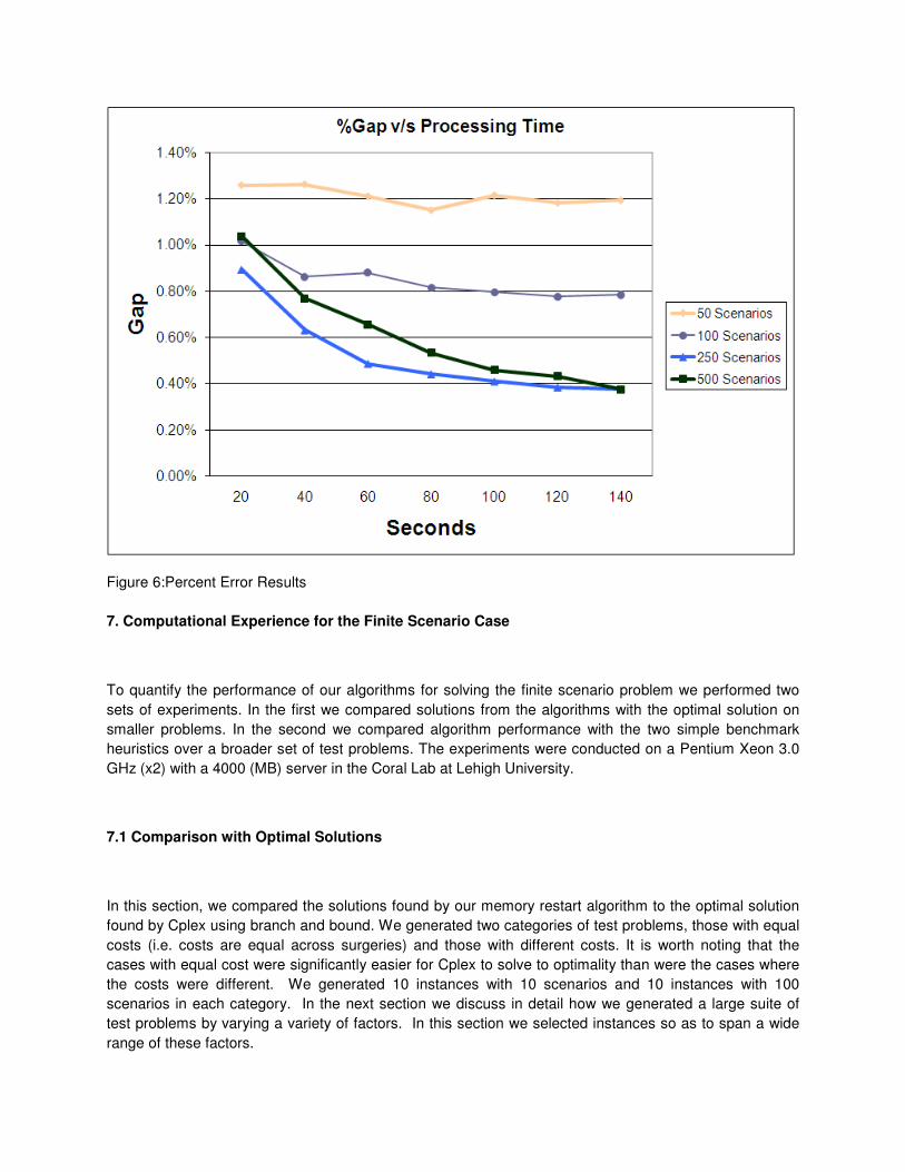
Figure 6:Percent Error Results

7. Computational Experience for the Finite Scenario Case

To quantify the performance of our algorithms for solving the finite scenario problem we performed two

sets of experiments. In the first we compared solutions from the algorithms with the optimal solution on

smaller problems. In the second we compared algorithm performance with the two simple benchmark

heuristics over a broader set of test problems. The experiments were conducted on a Pentium Xeon 3.0

GHz (x2) with a 4000 (MB) server in the Coral Lab at Lehigh University.

7.1 Comparison with Optimal Solutions

In this section, we compared the solutions found by our memory restart algorithm to the optimal solution

found by Cplex using branch and bound. We generated two categories of test problems, those with equal

costs (i.e. costs are equal across surgeries) and those with different costs. It is worth noting that the

cases with equal cost were significantly easier for Cplex to solve to optimality than were the cases where

the costs were different. We generated 10 instances with 10 scenarios and 10 instances with 100

scenarios in each category. In the next section we discuss in detail how we generated a large suite of

test problems by varying a variety of factors. In this section we selected instances so as to span a wide

range of these factors.

To find optimal solutions we used Cplex 10.2 to solve the strengthened IP formulation discussed in

subsection 3.2. Within Cplex the "MIP emphasis" parameter was set to "optimality". We ran our memory

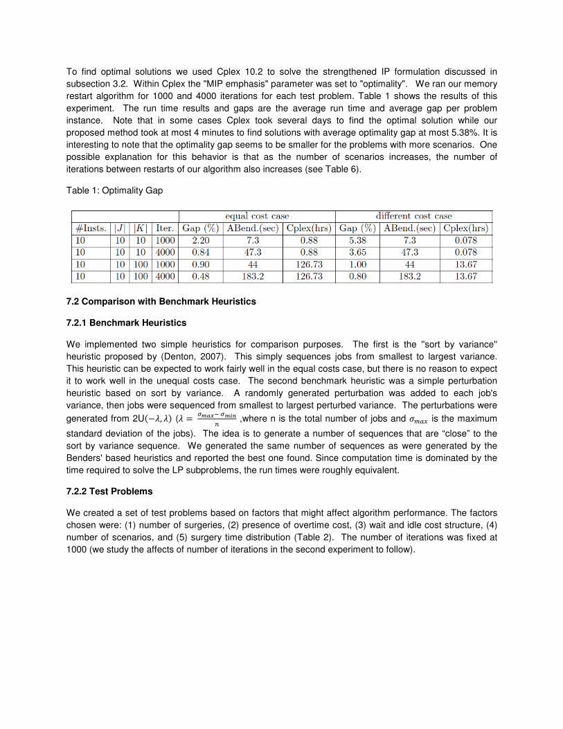
restart algorithm for 1000 and 4000 iterations for each test problem. Table 1 shows the results of this

experiment. The run time results and gaps are the average run time and average gap per problem

instance. Note that in some cases Cplex took several days to find the optimal solution while our

proposed method took at most 4 minutes to find solutions with average optimality gap at most 5.38%. It is

interesting to note that the optimality gap seems to be smaller for the problems with more scenarios. One

possible explanation for this behavior is that as the number of scenarios increases, the number of

iterations between restarts of our algorithm also increases (see Table 6).

Table 1: Optimality Gap

7.2 Comparison with Benchmark Heuristics

7.2.1 Benchmark Heuristics

We implemented two simple heuristics for comparison purposes. The first is the ''sort by variance''

heuristic proposed by (Denton, 2007). This simply sequences jobs from smallest to largest variance.

This heuristic can be expected to work fairly well in the equal costs case, but there is no reason to expect

it to work well in the unequal costs case. The second benchmark heuristic was a simple perturbation

heuristic based on sort by variance. A randomly generated perturbation was added to each job's

variance, then jobs were sequenced from smallest to largest perturbed variance. The perturbations were

generated from 2U012, 24 (2 5 6789: 67;<

= ,where n is the total number of jobs and >?@A is the maximum

standard deviation of the jobs). The idea is to generate a number of sequences that are “close” to the

sort by variance sequence. We generated the same number of sequences as were generated by the

Benders' based heuristics and reported the best one found. Since computation time is dominated by the

time required to solve the LP subproblems, the run times were roughly equivalent.

7.2.2 Test Problems

We created a set of test problems based on factors that might affect algorithm performance. The factors

chosen were: (1) number of surgeries, (2) presence of overtime cost, (3) wait and idle cost structure, (4)

number of scenarios, and (5) surgery time distribution (Table 2). The number of iterations was fixed at

1000 (we study the affects of number of iterations in the second experiment to follow).

Table 2: Experiment Design

Note that the indices 1,2,3,4 in the possible values of the factor Surgery Distribution are used as the

labels of Data in Figure 7.

The means and variances of surgery duration distributions were based on real data from a local hospital.

We then generated simulated surgery times from normal distributions (truncated at zero) with parameters

reflected in the real data.

In table 2 under surgery distribution the symbol B, > means all surgery durations were generated using

the same mean and standard deviation (186 , 66 ). The symbol B , > means that > was set at 66 and B

was set based on the coefficient of variation generated from a uniform(0.21,1.05)distribution. The symbol

B, > means that B was set at 186 then > was set based on the coefficient of variation generated from a

uniform(0.21,1.05) distribution. The symbol B , > means that B was first generated from uniform(90,300)

distribution then > was set based on a coefficient of variation generated from a uniform(0.21,1.05)

distribution.

In the equal cost case we generated a single waiting cost and idle cost each from a uniform (20,150)

distribution. These two costs were then applied to every surgery. In the unequal cost case individual idle

and waiting costs were generated for each surgery, again from a uniform (20,150) distribution.

When overtime is included, the over time cost is set to 1.5 times the average of the waiting costs. The

deadline was set equal to the sum (over surgeries) of the average (over scenarios) duration plus one

standard deviation (over scenarios) of this sum.

We created a full factorial experimental design and performed 5 replicates for each combination of factor

levels. This resulted in 1200 instances for each of the five algorithms tested: Approximate Benders'

Decomposition (with the three different restart rules), sort by variance, and perturbed sort by variance with

1000 iterations. We generated 1000 (not necessarily unique) sequences for each algorithm (except sort

be variance), solved the LP sub-problem for each to get the objective function, and report the best

solution found. Thus for each problem instance we have five solutions, one for each heuristic. We take

the best solution of these five, then compute the percent gap from this best solution for each heuristic for

each problem instance. The overall average gap results appear in table 3.

Table 3: Average percentage gap over the best solution found v/s scenarios

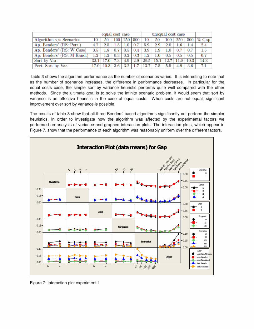
Table 3 shows the algorithm performance as the number of scenarios varies. It is interesting to note that

as the number of scenarios increases, the difference in performance decreases. In particular for the

equal costs case, the simple sort by variance heuristic performs quite well compared with the other

methods. Since the ultimate goal is to solve the infinite scenario problem, it would seem that sort by

variance is an effective heuristic in the case of equal costs. When costs are not equal, significant

improvement over sort by variance is possible.

The results of table 3 show that all three Benders' based algorithms significantly out perform the simpler

heuristics. In order to investigate how the algorithm was affected by the experimental factors we

performed an analysis of variance and graphed interaction plots. The interaction plots, which appear in

Figure 7, show that the performance of each algorithm was reasonably uniform over the different factors.

Overtime

Cost

Surgeries

Scenarios

Algor

Data

4321 201510 Sort Var iance

Per t Bench

App Ben Worst

App Ben Pert

App Ben Memory

0.30

0.15

0.000.30

0.15

0.000.30

0.15

0.000.30

0.15

0.000.30

0.15

0.00

10

0.30

0.15

0.00

10500

250

1005010

Overtime

0

1

Data

3

4

1

2

Cost

0

1

Surgeries

20

10

15

Scenarios

100

250

500

10

50

Algor

App Ben Worst

Pert Bench

Sort Variance

App Ben Memory

App Ben Pert

Interaction Plot (data means) for Gap

Figure 7: Interaction plot experiment 1

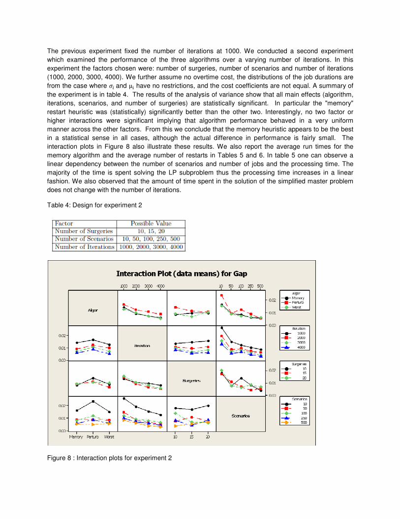
The previous experiment fixed the number of iterations at 1000. We conducted a second experiment

which examined the performance of the three algorithms over a varying number of iterations. In this

experiment the factors chosen were: number of surgeries, number of scenarios and number of iterations

(1000, 2000, 3000, 4000). We further assume no overtime cost, the distributions of the job durations are

from the case where > and µD have no restrictions, and the cost coefficients are not equal. A summary of

the experiment is in table 4. The results of the analysis of variance show that all main effects (algorithm,

iterations, scenarios, and number of surgeries) are statistically significant. In particular the "memory"

restart heuristic was (statistically) significantly better than the other two. Interestingly, no two factor or

higher interactions were significant implying that algorithm performance behaved in a very uniform

manner across the other factors. From this we conclude that the memory heuristic appears to be the best

in a statistical sense in all cases, although the actual difference in performance is fairly small. The

interaction plots in Figure 8 also illustrate these results. We also report the average run times for the

memory algorithm and the average number of restarts in Tables 5 and 6. In table 5 one can observe a

linear dependency between the number of scenarios and number of jobs and the processing time. The

majority of the time is spent solving the LP subproblem thus the processing time increases in a linear

fashion. We also observed that the amount of time spent in the solution of the simplified master problem

does not change with the number of iterations.

Table 4: Design for experiment 2

Figure 8 : Interaction plots for experiment 2

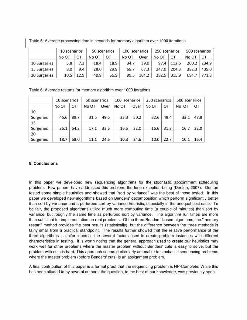
Table 5: Average processing time in seconds for memory algorithm over 1000 iterations.

10 scenarios 50 scenarios 100 scenarios 250 scenarios 500 scenarios

No OT OT No OT OT No OT Over No OT OT No OT OT

10 Surgeries 5.8 7.3 18.4 18.9 34.7 39.0 97.4 112.6 200.2 234.9

15 Surgeries 8.0 9.4 28.0 29.9 69.7 67.3 247.0 204.3 382.3 435.0

20 Surgeries 10.5 12.9 40.9 56.9 99.5 104.2 282.5 315.9 694.7 771.8

Table 6: Average restarts for memory algorithm over 1000 iterations.

10 scenarios 50 scenarios 100 scenarios 250 scenarios 500 scenarios

No OT OT No OT Over No OT Over No OT OT No OT OT

10

Surgeries 46.6 89.7 31.5 49.5 33.3 50.2 32.6 49.4 33.1 47.8

15

Surgeries 26.1 64.2 17.1 33.5 16.5 32.0 16.6 31.3 16.7 32.0

20

Surgeries 18.7 68.0 11.1 24.5 10.3 24.6 10.0 22.7 10.1 16.4

8. Conclusions

In this paper we developed new sequencing algorithms for the stochastic appointment scheduling

problem. Few papers have addressed this problem, the lone exception being (Denton, 2007). Denton

tested some simple heuristics and showed that "sort by variance" was the best of those tested. In this

paper we developed new algorithms based on Benders' decomposition which perform significantly better

than sort by variance and a perturbed sort by variance heuristic, especially in the unequal cost case. To

be fair, the proposed algorithms utilize much more computing time (a couple of minutes) than sort by

variance, but roughly the same time as perturbed sort by variance. The algorithm run times are more

than sufficient for implementation on real problems. Of the three Benders' based algorithms, the "memory

restart" method provides the best results (statistically), but the difference between the three methods is

fairly small from a practical standpoint. The results further showed that the relative performance of the

three algorithms is uniform across the several factors used to create problem instances with different

characteristics in testing. It is worth noting that the general approach used to create our heuristics may

work well for other problems where the master problem without Benders' cuts is easy to solve, but the

problem with cuts is hard. This approach seems particularly amenable to stochastic sequencing problems

where the master problem (before Benders' cuts) is an assignment problem.

A final contribution of this paper is a formal proof that the sequencing problem is NP-Complete. While this

has been alluded to by several authors, the question, to the best of our knowledge, was previously open.

References Aardal, K., T. Larsson. 1990. A benders decomposition based heuristic for the hierarchical production planning problem. European Journal of Operational Research 45(1) 4 - 14. Mehmet A. Begen and Maurice Queyranne. Appointment scheduling with discrete random durations. Under review (A version of this paper appeared in the proceedings of the Symposium on Discrete Algorithms 2009 (SODA09), University of Western Ontario, 2010a. Caroe, C. C., R. Schultz. 1999. Dual decomposition in stochastic integer programming. Operations Research Letters (24) 37 - 45. Cote, G., M. A. Laughton. 1984. Large-scale mixed integer programming: Benders-type heuristics. European Journal of Operational Research 16(3) 327 - 333. Denton, B., D. Gupta. 2003. Sequential bounding approach for optimal appointment scheduling. IIE Transactions 35 (11) 1003-1016. Denton, B., J. Viapiano, A. Vogl. 2007. Optimization of surgery sequencing and scheduling decisions under uncertainty. Health Care Management Science (10) Garey, M.R., D. S. Johnson, R. Sethi. 1976. The complexity of flowshop and jobshop scheduling. Math. Of Operations Research (1) 117-129. Gupta, D. 2007. Surgical suites operations management. Production and Operations Management 16 (6) 689 - 700. HFMA. 2005. Achieving operating room efficiency through process integration. Health Care Financial Management Association Report . Kaandorp, G. C., G. Koole. 2007. Optimal outpatient appointment scheduling. Health Care Manage Science 10 217 - 229. Kleywegt, A., A. Shapiro, T. Homem de Mello. 2002. The sample average approximation method for stochastic discrete optimization. SIAM Journal on Optimization (12) 479 - 502. Laporte, G., F.V. Louveaux. 1993. The integer l-shaped method for stochastic integer programs with complete recourse. Operations research letters (13) 133 - 142. Linderoth, J. T., A. Shapiro, S. J. Wright. 2006. The empirical behavior of sampling methods for stochastic programming. Annals of Operations Research 142 219{245. Mancilla, C., R. H. Storer. 2009. Stochastic sequencing and scheduling of an operating room. Tech. rep., Industrial and System Engineering, Lehigh University. Norkin, V., Y. Ermoliev, A. Ruszczynski. 1998. On optimal allocation of indivisibles under uncertainty. Operations Research 46(3) 381. Kong Qingxia, Chung-Yee Lee, Chung-Piaw Teo and Zhichao Zheng. 2010. Scheduling Arrivals to a Stochastic Service Delivery System using Copositive Cones, working paper. Robinson, L.W., R. R. Chen. 2003. Scheduling doctors appointments: Optimal and empirically-based heuristic policies. IIE Transactions 35 295 - 307. Schultz, R. 2003. Stochastic programming with integer variables. Mathematical Programming 97 285 -309. Storer, R. H., D. S. Wu, R. Vaccari. 1992. New search spaces for sequencing problems with application to job shop scheduling. Management Science 38(10) 1495 - 1509. Vanden Bosch, P. M., D. C. Dietz. 2000. Minimizing expected waiting in a medical appointment system.IIE Transactions 32 841 - 848. Vanden Bosch, P. M., D. C. Dietz. 2001. Scheduling and sequencing arrivals to an appointment system. Journal of Service Research 4 (1) 1525. Wang, P. Patrick. 1997. Optimally scheduling n customer arrival times for a single-server system. Computers & Operations Research 24(8) 703 - 716. Weiss, E.N. 1990. Models for determining the estimated start times and case orderings. IIE Transactions 22 (2) 143 - 150.