Embed Size (px)
Citation preview

Exact Controllability and Stabilization.
The Multiplier Method
Vilmos Komornik
Universite Louis Pasteur, Strasbourg
v
Icanak, Timinek es Zsoltnak
PREFACE
This book grew out of a series of lectures given over the past four years in
France, Hungary and the USA.
In the first part exact boundary controllability problems are studied by
the Hilbert Uniqueness Method. This approach, introduced by LIONS [3] in
1986, is based on uniqueness theorems leading to the construction of suitable
Hilbert spaces of the controllable spaces. It is closely related to a duality
theory of DOLECKI AND RUSSELL [1]. Following HO [1] and LIONS [2], these
spaces may often be characterized by using the multiplier method. In chapters
2 to 4 we reproduce some results of LIONS [4], [5] with certain changes :
– some compactness–uniqueness arguments are replaced by constructive
proofs ;
– equations containing lower-order terms are also considered ;
– more general boundary conditions are used which in fact simplify the
theory.
The results of chapters 5 and 6 were obtained after the publication of Lions’
monography. In chapter 5 we develop a general and constructive approach to
improve the usual estimates of the exact controllability time. It was inspired
by a new estimation method of HARAUX [3]. Using this approach, in chapter
6 we improve most of the results obtained in chapters 3 and 4. We also give
elementary and constructive proofs for certain results of ZUAZUA [1], obtained
earlier by indirect arguments.
The second part of the book is devoted to stabilizability. In chapters 8 and 9
strong and uniform boundary stabilization theorems are proved. Our method
is a modified and simplified version of a Liapunov type approach introduced
in KOMORNIK AND ZUAZUA [1]. We also present here a classical principle of
RUSSELL [2] connecting the exact controllability to the stabilizability, and
some recent results of CONRAD AND RAO [1].
For the sake of brevity in the first nine chapters we consider only the
wave equation, Maxwell’s equations and very simple plate models. In the
last chapter we consider the internal stabilization of the Korteweg–de Vries
equation : we prove a special case of a theorem in KOMORNIK, RUSSELL AND
ZHANG [2].
The multiplier method, applied systematically in this book, is remarkably
elementary and efficient. In the bibliography we have included some references
vi
which use other approaches : see in particular the work of Bardos et al.,
Littmann, Russell, Joo and their references. We have also included some
material concerning other equations.
I wish to express my gratitude to
– J.-L. Lions for his advice and numerous suggestions concerning the
subject of this book, for his valuable remarks on a preliminary version of
these notes and for his proposal to publish it in the collection RMA;
– P. G. Ciarlet who also proposed the publication of this book in this
collection and who gave me useful advice concerning the presentation of the
material ;
– F. Conrad, A. Haraux, J. Lagnese, B. Rao, D. L. Russell and E. Zuazua
for many fruitful discussions ;
– the Mathematical Departments of Virginia Tech, the Universities of
Strasbourg I, Nancy I, the Eotvos University of Budapest and the Institute
of Mathematics and its Applications at the University of Minnesota, where
my lectures were given and/or part of this book was written ;
– the students and colleagues following my lectures, in particular S.
Kouemou-Patcheu who read the manuscript and made a number of useful
remarks.
Strasbourg, November 29, 1993
vii
TABLE OF CONTENTS
Preface . . . . . . . . . . . . . . . . . . . . . . . . v
0. Introduction. Vibrating strings . . . . . . . . . . . . . 1
1. Linear evolutionary problems . . . . . . . . . . . . . . 7
1.1. The diagram V ⊂ H = H ′ ⊂ V ′ . . . . . . . . . . . . . . . . 7
1.2. The equation u′′ + Au = 0 . . . . . . . . . . . . . . . . . . 10
1.3. The wave equation . . . . . . . . . . . . . . . . . . . . . 11
1.4. A Petrovsky system . . . . . . . . . . . . . . . . . . . . . 13
1.5. Another Petrovsky system . . . . . . . . . . . . . . . . . . 15
2. Hidden regularity. Weak solutions . . . . . . . . . . . 18
2.1. A special vector field . . . . . . . . . . . . . . . . . . . . . 18
2.2. The wave equation. Multiplier method . . . . . . . . . . . . . 19
2.3. The first Petrovsky system . . . . . . . . . . . . . . . . . . 24
2.4. The second Petrovsky system . . . . . . . . . . . . . . . . . 29
3. Uniqueness theorems . . . . . . . . . . . . . . . . 35
3.1. The wave equation. Dirichlet condition . . . . . . . . . . . . . 35
3.2. The first Petrovsky system . . . . . . . . . . . . . . . . . . 40
3.3. The second Petrovsky system . . . . . . . . . . . . . . . . . 44
3.4. The wave equation. Mixed boundary conditions . . . . . . . . . 47
4. Exact controllability. Hilbert uniqueness method . . . . 53
4.1. The wave equation. Dirichlet control . . . . . . . . . . . . . . 53
4.2. The first Petrovsky system . . . . . . . . . . . . . . . . . . 57
4.3. The wave equation. Neumann or Robin control . . . . . . . . . 59
5. Norm inequalities . . . . . . . . . . . . . . . . . . 63
5.1. Riesz sequences . . . . . . . . . . . . . . . . . . . . . . . 63
5.2. Formulation of the results . . . . . . . . . . . . . . . . . . 65
5.3. Proof of theorem 5.3 . . . . . . . . . . . . . . . . . . . . . 69
5.4. Proof of theorem 5.5 . . . . . . . . . . . . . . . . . . . . . 73
6. New uniqueness and exact controllability results . . . . . 75
6.1. A unique continuation theorem . . . . . . . . . . . . . . . . 75
6.2. The wave equation. Dirichlet condition . . . . . . . . . . . . . 77
6.3. The first Petrovsky system . . . . . . . . . . . . . . . . . . 79
viii
6.4. The second Petrovsky system. Uniqueness theorems . . . . . . . 81
6.5. The second Petrovsky system. Exact controllability . . . . . . . 83
6.6. The wave equation. Neumann or Robin condition . . . . . . . . 85
7. Dissipative evolutionary systems . . . . . . . . . . . 90
7.1. Maximal monotone operators . . . . . . . . . . . . . . . . . 90
7.2. The wave equation . . . . . . . . . . . . . . . . . . . . . 91
7.3. Kirchhoff plates . . . . . . . . . . . . . . . . . . . . . . . 97
8. Linear stabilization . . . . . . . . . . . . . . . . . 103
8.1. An integral inequality . . . . . . . . . . . . . . . . . . . 103
8.2. Uniform stabilization of the wave equation I . . . . . . . . . 104
8.3. Links with the exact controllability. Russell’s principle . . . . . 108
8.4. Uniform stabilization of the wave equation II . . . . . . . . . 111
8.5. Strong stabilization. LaSalle’s principle . . . . . . . . . . . . 114
8.6. Uniform stabilization of the wave equation III . . . . . . . . . 116
8.7. Uniform stabilization of Maxwell’s equations . . . . . . . . . 118
9. Nonlinear stabilization . . . . . . . . . . . . . . . . 124
9.1. A nonlinear integral inequality . . . . . . . . . . . . . . . 124
9.2. Uniform stabilization of the wave equation I . . . . . . . . . 126
9.3. Uniform stabilization of the wave equation II . . . . . . . . . 134
9.4. Uniform stabilization of Kirchhoff plates . . . . . . . . . . . 135
10. Internal stabilization of the Korteweg–de Vries equation . 144
10.1. Well-posedness and conservation laws . . . . . . . . . . . . 144
10.2. Uniform stabilization by linear feedbacks . . . . . . . . . . 146
References . . . . . . . . . . . . . . . . . . . . . . 152
Vibrating strings 1
0. Introduction. Vibrating strings
Let I = (a, b) be a bounded interval, T a positive number and consider
the following problem, modelling among other things the small transversal
vibrations of a string :
(utt − uxx)(x, t) = 0, (x, t) ∈ I × (0, T ), (1)
u(a, t) = va(t) and u(b, t) = vb(t), t ∈ [0, T ], (2)
u(x, 0) = u0(x) and ut(x, 0) = u1(x), x ∈ I. (3)
The problem (1)–(3) is said to be exactly controllable if for ”arbitrarily”
given initial ”state” (u0, u1) there exist suitable ”control” functions va and
vb such that the solution of (1)–(3) satisfies
u(x, T ) = ut(x, T ) = 0, x ∈ I. (4)
We say that the controls va and vb drive the system to rest in time T .
Naturally, we have to specify the functional spaces of the initial states and
of the controls ; the results depend on these choices.
The solution of (1)–(3) is by definition a function
u ∈ C([0, T ];H1(I)) ∩ C1([0, T ];L2(I)) (5)
satisfying (1) in the distributional sense, the equalities (2) pointwise, and the
equalities (3) almost everywhere. (As for the usual properties of the Sobolev
spaces applied in this book we refer e.g. to LIONS AND MAGENES [1].)
We have the following result :
THEOREM 0.1. — Let T = b − a and let (u0, u1) ∈ H1(I) × L2(I) be such
that
u0(a) + u0(b) +
∫ b
a
u1(s) ds = 0. (6)
Then there is a unique choice of functions
va, vb ∈ H1(0, T ) (7)
such that the solution of (1)–(3) satisfies (4).
Moreover, va and vb are given by the formulae
2va(t) = u0(a + t) + u0(a) +
∫ a+t
a
u1(s) ds, (8)
2 0. Introduction
2vb(t) = u0(b − t) + u0(b) +
∫ b
b−t
u1(s) ds (9)
and the solution u has the following supplementary property :
u(a, t) + u(b, t) +
∫ b
a
ut(s, t) ds = 0, ∀t ∈ [0, T ]. (10)
PROOF. — Applying d’Alembert’s formula the solutions of (1) may be written
in the form
u(x, t) ≡ f(x + t) + g(x − t) (11)
with suitable functions f : (a, b + T ) → R and g : (a − T, b) → R. Using (2)
and (3) we obtain that
f(a + t) + g(a − t) = va(t), t ∈ (0, T ), (12)
f(b + t) + g(b − t) = vb(t), t ∈ (0, T ), (13)
f(x) + g(x) = u0(x), x ∈ I, (14)
f ′(x) − g′(x) = u1(x), x ∈ I. (15)
We deduce from (14), (15) that
2f(x) = u0(x) + U1(x), x ∈ I (16)
and
2g(x) = u0(x) − U1(x), x ∈ I, (17)
where U1 is a suitable primitive of u1.
We conclude from (12) and (16) that
2g(a − t) = 2va(t) − u0(a + t) − U1(a + t), 0 < t < b − a;
similarly, we conclude from (13) and (17) that
2f(b + t) = 2vb(t) − u0(b − t) + U1(b − t), 0 < t < b − a;
we can rewrite these relations in the following form :
2g(s) = 2va(a − s) − (U1 + u0)(2a − s), 2a − b < s < a, (18)
2f(s) = 2vb(s − b) + (U1 − u0)(2b − s), b < s < 2b − a. (19)
Vibrating strings 3
We deduce from (11), (18) and (19) that for
a < x < b and maxx − a, b − x < t < b − a (20)
we have
2u(x, t) = 2va(a + t − x) + 2vb(x + t − b)
(21)
−u0(2a − x + t) − u0(2b − x − t) +
∫ 2b−x−t
2a−x+t
u1(s) ds.
We have in particular
u(x, b − a) = va(b − x) + vb(x − a) − u0(a + b − x), x ∈ I
and
ut(x, b − a) = v′a(b − x) + v′
b(x − a) − u1(a + b − x), x ∈ I.
Thus the final conditions (4) are equivalent to
va(b − x) + vb(x − a) = u0(a + b − x), x ∈ I
and
−va(b − x) + vb(x − a) = −V 1(a + b − x), x ∈ I
with an arbitrary primitive V 1 of u1 whence
2va(b − x) = (u0 + V 1)(a + b − x), x ∈ I,
2vb(x − a) = (u0 − V 1)(a + b − x), x ∈ I,
or
2va(t) = (u0 + V 1)(a + t), 0 < t < b − a, (22)
2vb(t) = (u0 − V 1)(b − t), 0 < t < b − a. (23)
Let us introduce the subsets U,R,D,L of I × (0, T ) ( the letters mean
”Up”, ”Right”, ”Down”, ”Left”) defined by
U := (x, t) ∈ I × (0, T ) : t > x − a et t > b − x,R := (x, t) ∈ I × (0, T ) : b − x < t < x − a,
D := (x, t) ∈ I × (0, T ) : t < x − a et t < b − x,L := (x, t) ∈ I × (0, T ) : x − a < t < b − x.
4 0. Introduction
One can easily deduce from (11), (16)–(19), (22) and (23) the following
formulae :
2u(x, t) =
0, if (x, t) ∈ U ;
(u0 − V 1)(x − t), if (x, t) ∈ R ;
u0(x + t) + u0(x − t) +∫ x+t
x−tu1(s) ds, if (x, t) ∈ D ;
(u0 + V 1)(x + t), if (x, t) ∈ L.
(24)
Comparing the limits of these formulae at t = x − a and t = b − x we
obtain that for any fixed 0 < t < T , t 6= T/2, the function x 7→ u(x, t) is
continuous only if
V 1(a) = u0(a) and V 1(b) = −u0(b). (25)
By hypothesis (6) u1 has a unique primitive V 1 with this property. Choosing
V 1 in this way, (22), (23) follow from (8), (9), and we deduce from (24) that
2u(x, t) =
0, if (x, t) ∈ U ;
u0(x − t) + u0(b) +∫ b
x−tu1(s) ds, if (x, t) ∈ R ;
u0(x + t) + u0(x − t) +∫ x+t
x−tu1(s) ds, if (x, t) ∈ D ;
u0(x + t) + u0(a) +∫ x+t
au1(s) ds, if (x, t) ∈ L ;
(26)
using these formulae one can directly verify (5) and (10).
REMARK 0.2. — The problem (1)–(3) is also exactly controllable if
T > b− a. Indeed, it is sufficient to drive the system to rest in time b− a and
then to extend the control functions va, vb by zero for b − a < t < T . Since
va(b − a) = vb(b − a) = 0 by (6), (8) and (9), the property (7) remains valid.
REMARK 0.3. — The problem (1)–(3) is not exactly controllable if T < b−a.
Indeed, assume that the system may be driven to rest in time T from some
given initial data u0, u1. Extending the corresponding controls va, vb by zero
for T < t < b − a, we obtain that the system may be driven from the initial
state (u0, u1) to rest in time b−a with controls va, vb ∈ L2(0, b−a) satisfying
va = vb ≡ 0 in some left neighbourhood of b − a. (27)
On the other hand, the proof of theorem 0.1 (see (22) and (23)) shows that
2va(t)+2vb(t) = u0(a+ t)+u0(b− t)+
∫ a+t
b−t
u1(s) ds, 0 < t < b−a. (28)
But (27) and (28) are not satisfied simultaneously for all initial data
(u0, u1) ∈ H1(I) × L2(I) satisfying (6).
Vibrating strings 5
The following result improves theorem 0.1 by driving the system to general
final states :
THEOREM 0.4. — Let T = b − a, (u0, u1), (u0T , u1
T ) ∈ H1(I) × L2(I) and
assume that
u0(a) + u0(b) +
∫ b
a
u1(s) ds = 0 and u0T (a) + u0
T (b) +
∫ b
a
u1T (s) ds = 0.
Then there exist unique functions va, vb ∈ H1(0, T ) such that the solution of
(1)–(3) satisfies
u(x, T ) = u0T (x) and ut(x, T ) = u1
T (x), x ∈ I. (29)
PROOF. — First we solve the problem
(ztt − zxx)(x, t) = 0, (x, t) ∈ I × (0, T ),
z(a, t) = z(b, t) = 0, t ∈ (0, T ),
z(x, T ) = u0T (x) and zt(x, T ) = u1
T (x), x ∈ I,
and then we choose (using theorem 0.1) va and vb such that the solution of
the problem
(ytt − yxx)(x, t) = 0, (x, t) ∈ I × (0, T ),
y(a, t) = va(t), y(b, t) = vb(t), t ∈ (0, T ),
y(x, 0) = u0(x) − z(x, 0) and yt(x, 0) = u1(x) − zt(x, 0), x ∈ I
satisfies
y(x, T ) = yt(x, T ) = 0, x ∈ I.
Then u := y + z is the solution of (1)–(3) and it satisfies (29).
Let us return to theorem 0.1. From the point of view of applications
it would be useful to find controls va, vb defined by some ”feedback law”
va = Fa(u), vb = Fb(u) with explicitly given functions Fa, Fb : this would
realize an ”automatic” control of the system. For the problem (1)–(3) such
feedbacks can be found easily : let us consider the problem
(utt − uxx)(x, t) = 0, (x, t) ∈ I × R+, (30)
(ux − ut)(a, t) = (ux + ut)(b, t) = 0, t ∈ R+, (31)
u(x, 0) = u0(x) and ut(x, 0) = u1(x), x ∈ I. (32)
6 0. Introduction
By definition, a solution of this problem is a function
u ∈ C([0,+∞]; H1(I)) ∩ C1([0,+∞]; L2(I))
satisfying (30) in the distributional sense, (32) almost everywhere and (31) in
the following sense : in some neighbourhood of a × R+ u(x, t) is a function
of x + t and in some neighbourhood of b × R+ it is a function of x − t.
THEOREM 0.5. — Let (u0, u1) ∈ H1(I) × L2(I) be such that
u0(a) + u0(b) +
∫ b
a
u1(s) ds = 0. (33)
Then the solution of (30)–(32) satisfies
u(x, t) = 0, ∀(x, t) ∈ I × [b − a,+∞). (34)
PROOF. — Adapting the proof of theorem 0.1 we obtain that the solution of
(30)–(32) has again the form (11) with suitable functions f : (a,+∞) → R et
g : (−∞, b) → R satisfying (14), (15) and
g′(a − t) = 0, t ∈ R+, (35)
f ′(b + t) = 0, t ∈ R+. (36)
It follows that f , g satisfy (16), (17) with a suitable primitive U1 of u1, and
that
g(s) = g(a), s ≤ a, (37)
f(s) = f(b), s ≥ b. (38)
Introducing the subsets U , R, D, L as before, but replacing T by +∞, we
deduce from (11), (16), (17), (37) and (38) the following formulae :
2u(x, t) =
u0(a) + u0(b) +∫ b
au1(s) ds, if (x, t) ∈ U ;
u0(x − t) + u0(b) +∫ b
x−tu1(s) ds, if (x, t) ∈ R ;
u0(x + t) + u0(x − t) +∫ x+t
x−tu1(s) ds, if (x, t) ∈ D ;
u0(x + t) + u0(a) +∫ x+t
au1(s) ds, if (x, t) ∈ L.
(39)
These show in particular the uniqueness of the solution of (30)–(32).
One can verify by a direct computation that the function defined by (39)
is indeed a solution of (30)–(32). Finally, (34) follows from (33) and (39).
1.1. The diagram V ⊂ H = H ′ ⊂ V ′ 7
1. Linear evolutionary problems
The results of this chapter are standard ; see e.g. LIONS AND MAGENES [1]
for proof.
1.1. The diagram V ⊂ H = H′ ⊂ V′
Let V be an infinite-dimensional, separable, real or complex Hilbert space
and introduce the duality mapping A : V → V ′ defined by
〈Au, v〉V ′,V := (u, v)V , u, v ∈ V. (1)
By the Riesz-Frechet representation theorem A is an isometric isomorphism
of V onto V ′.
Let H be another Hilbert space with a dense and compact imbedding
V ⊂ H. (The compactness means that every bounded subset of V is
precompact in H.) Then in addition H is of infinite dimension, separable,
and the imbedding H ′ ⊂ V ′ is also dense and compact. Identifying H with
H ′, we obtain the diagram
V ⊂ H = H ′ ⊂ V ′. (2)
We deduce from (1) that
(Au, v)H = (u, v)V , ∀u ∈ V such that Au ∈ H, ∀v ∈ V. (3)
Denoting by i the compact imbedding of V into V ′, the linear map
T := A−1 i : V → V is also compact. Moreover, it is selfadjoint. Indeed,
given u, v ∈ V arbitrarily, we deduce from (3) that
(Tu, v)V = (A−1u, v)V = (u, v)H
and
(u, Tv)V = (u,A−1v)V = (u, v)H ,
whence
(Tu, v)V = (u, Tv)V .
8 1. Linear evolutionary problems
Applying the spectral theorem to T = A−1 i we conclude that there exists
a sequence λ1, λ2,. . . of distinct real numbers (the eigenvalues of A) and a
sequence Z1, Z2,. . . of subspaces of V such that
|λk| → +∞,
Az = λkz, ∀z ∈ Zk, ∀k ≥ 1, (4)
dim Zk < +∞, ∀k ≥ 1, (5)
Zk ⊥ Zl in V if k 6= l, (6)
and
the vector space Z generated by ∪ Zk is dense in V. (7)
It follows from (3) and (4) that the eigenvalues are positive. We may thus
assume that
0 < λ1 < λ2 < · · · and λk → +∞. (8)
It follows from (6) and (7) that every v ∈ V has a unique orthogonal
expansion
v =∑
vk, vk ∈ Zk, ∀k ≥ 1, (9)
converging in V ; furthermore, we deduce from (6), (9), (3) and (4) that
‖v‖2V =
∑‖vk‖2
V =∑
λk‖vk‖2H . (10)
Now observe that
Zk ⊥ Zl in H and also in V ′ if k 6= l. (11)
Indeed, the orthogonality in H follows from (3), (4), (6) and (8), while the
orthogonality in V ′ follows from (4) and (6), using the isometric property of
A : for u ∈ Zk and v ∈ Zl, k 6= l, we have
(u, v)V ′ = (A−1u,A−1v)V = λ−1k λ−1
l (u, v)V = 0.
Next we deduce from (9) and from the density of the imbeddings in (2) that
Z is also dense in H and in V ′. Therefore every v ∈ H (resp. every v ∈ V ′)
1.1. The diagram V ⊂ H = H ′ ⊂ V ′ 9
has a unique orthogonal expansion of the form (9), converging in H (resp. in
V ′), and we have
‖v‖2H =
∑‖vk‖2
H (12)
(resp.
‖v‖2V ′ =
∑‖vk‖2
V ′ =∑
λ−1k ‖vk‖2
H). (13)
The last equality of (13) follows from (10) :
‖vk‖2V ′ = ‖A−1vk‖2
V = λ−2k ‖vk‖2
V = λ−1k ‖vk‖2
H .
Let α ∈ R and define a euclidean norm ‖ · ‖α on Z by putting
‖v‖α :=(∑
λ2αk ‖vk‖2
H
)1/2
(here we use the expansion (9) of v). Completing Z with respect to this norm
we obtain a Hilbert space which will be denoted by Dα. It is easy to verify
the orthogonality relations
Zk ⊥ Zl dans Dα si k 6= l.
It is clear that for α > β the norm ‖ · ‖α is stronger than ‖ · ‖β . Thus we
may assume that
Dα ⊂ Dβ if α > β,
with a dense and continuous imbedding. (One can readily verify that these
imbeddings are in fact compact.) Set
D−∞ := ∪αDα.
For each fixed real number α let us introduce a linear mapping
Aα : D−∞ → D−∞ in the following way : first, for v ∈ Z given by (9)
we set
Aαv :=∑
λαk vk. (14)
Then for any given v ∈ D−∞ we choose β ∈ R such that v ∈ Dβ and then we
choose a sequence (vj) in Z such that ‖v − vj‖β → 0. One can readily verify
that Aαvj is a Cauchy sequence in Dβ−α, hence it converges to a certain
w ∈ Dβ−α. Furthermore, it is easy to show that the limit w is independent of
the particular choice of β and of the sequence vj . Define Aαv := w. It is clear
that for v ∈ Z this definition reduces to (14).
10 1. Linear evolutionary problems
The following properties are easy to verify :
Given α, β ∈ R arbitrarily, the restriction of Aα to Dβ is an isometric
isomorphism of Dβ onto Dβ−α.
We have AαAβ = Aα+β for all α, β ∈ R.
We have
‖v‖1/2 = ‖v‖V , ‖v‖0 = ‖v‖H and ‖v‖−1/2 = ‖v‖V ′
for every v ∈ Z.
As a consequence, using also the density of Z in V , H and in V ′, we may
identify D1/2 with V , D0 with H and D−1/2 with V ′. Then A1 is an extension
of A onto D−∞. In the sequel we shall also denote this extension by A i.e. we
shall write A instead of A1.
1.2. The equation u′′ + Au = 0
Let us first consider the homogeneous evolutionary problem
u′′ + Au = 0 dans R, u(0) = u0 et u′(0) = u1 (15)
with arbitrarily given initial data u0, u1 ∈ D−∞. We shall use the orthogonal
expansion of u0 and u1 :
u0 =∞∑
k=1
u0k and u1 =
∞∑
k=1
u1k, u0
k, u1k ∈ Zk, k = 1, 2, . . . (16)
THEOREM 1.1. — Let α ∈ R and (u0, u1) ∈ Dα+1/2 ×Dα. Then the problem
(15) has a unique solution such that
u ∈ C(R; Dα+1/2) ∩ C1(R; Dα) ∩ C2(R; Dα−1/2); (17)
it is given by the series
u(t) =∞∑
k=1
u0k cos(
√λkt) + u1
k
sin(√
λkt)√λk
, t ∈ R. (18)
The energy Eα : R → R+ of the solution, defined by
Eα(t) := 12‖u(t)‖2
α+1/2 + 12‖u′(t)‖2
α, (19)
1.2. The equation u′′ + Au = 0 11
is in fact independent of t ∈ R.
The linear mapping (u0, u1) 7→ u is continuous from Dα+1/2 × Dα into
Cb(R;Dα+1/2) ∩ C1b (R;Dα) ∩ C2
b (R;Dα−1/2).
Since the energy is independent of t ∈ R, we shall often write Eα(u)
instead of Eα(u0, u1).
Let us recall that for α = 0 we have Dα+1/2 = V , Dα = H and
Dα−1/2 = V ′. In this case we shall write E instead of E0.
REMARK 1.2. — The formula (18) shows that if u0 ⊥ Zk and u1 ⊥ Zk,
then u(t) ⊥ Zk and u′(t) ⊥ Zk for all t ∈ R. Since the equation (15) is
autonomous, we conclude more generally that if u(T ) ⊥ Zk and u′(T ) ⊥ Zk
for some T ∈ R, then necessarily u(t) ⊥ Zk and u′(t) ⊥ Zk for all t ∈ R.
REMARK 1.3. — One can readily verify that if (u0, u1) ∈ Dα+1/2 × Dα for
some α ∈ R and if u is the corresponding solution of (15), then for any fixed
β ∈ R, Aβu is the solution of (15) with (u0, u1) replaced by
(Aβu0, Aβu1) ∈ ×Dα−β+1/2 × Dα−β .
1.3. The wave equation
Let Ω be a bounded domain (that is, a non-empty open connected set)
of class C2 in Rn ; we denote by ν the outward unit normal vector to its
boundary Γ. Let Γ0,Γ1 be a partition of Γ (the cases Γ0 = ∅ or Γ1 = ∅are not excluded) and let q : Ω → R, a : Γ1 → R be two given nonnegative
functions.
We consider the problem
u′′ − ∆u + qu = 0 in Ω × R, (20)
u = 0 on Γ0 × R, (21)
∂νu + au = 0 on Γ1 × R, (22)
u(0) = u0 and u′(0) = u1. (23)
In order to avoid some difficulties (studied in detail by GRISVARD [1]), we
shall assume throughout this book that
Γ0 ∩ Γ1 = ∅ (24)
12 1. Linear evolutionary problems
and that
q ∈ L∞(Ω), a ∈ C1(Γ1). (25)
We introduce two real or complex Hilbert spaces H and V by the formulae
H := v ∈ L2(Ω) :
∫
Ω
v dx = 0,
(26)
V := v ∈ H1(Ω) :
∫
Ω
v dx = 0
if Γ0 = ∅, q ≡ 0 and a ≡ 0, and
H := L2(Ω) and V := H1(Ω) (27)
otherwise ; in both cases we define their norms by
‖v‖H :=(∫
Ω
|v|2 dx)1/2
(28)
and
‖v‖V :=(∫
Ω
|∇v|2 + q|v|2 dx +
∫
Γ1
a|v|2 dΓ)1/2
. (29)
One can readily verify that the seminorm ‖ · ‖V is indeed a norm and that it
is equivalent to the norm induced by H1(Ω). Applying Rellich’s theorem it
follows that the imbedding V ⊂ H is dense and compact.
We introduce the corresponding linear map A and we define the solution
of (20)-(23) as the (unique) solution of the problem
u′′ + Au = 0 in R, u(0) = u0, u′(0) = u1 (30)
in the sense of theorem 1.1. We justify this definition by showing that every
sufficiently smooth classical solution of (20)-(23) (for example of class C2 on
Ω × R) is also a solution of (30).
Fixing t ∈ R and v ∈ V arbitrarily, we have
0 =
∫
Ω
(u′′ − ∆u + qu)v dx
=
∫
Ω
u′′v + ∇u∇v + quv dx −∫
Γ
∂νuv dΓ
=
∫
Ω
(u′′ + qu)v + ∇u∇v dx +
∫
Γ1
auv dΓ
= 〈u′′, v〉V ′,V + (u, v)V = 〈u′′ + Au, v〉V ′,V
1.3. The wave equation 13
on R ; hence u′′(t) + Au(t) = 0 (as an element of V ′) for every t ∈ R.
Let us note that Au = −∆u + qu for every u ∈ V ∩ H2(Ω). Indeed, we
have for every v ∈ V the following equality :
∫
Ω
(−∆u + qu)v dx =
∫
Ω
∇u∇v + quv dx −∫
Γ
∂νuv dΓ
=
∫
Ω
∇u∇v + quv dx +
∫
Γ1
auv dΓ = 〈Au, v〉V ′,V .
We remark that for this choice of H, V and A the energy of the solutions
of (30) is given by the formula
E(t) := 12
∫
Ω
|u′(t)|2 + |∇u(t)|2 + q|u(t)|2 dx + 12
∫
Γ1
a|u(t)|2 dΓ. (31)
REMARK 1.4. — We recall from the elliptic regularity theory that under
conditions (24) and (25) for any given g ∈ L2(Ω) the solution v ∈ V of the
problem
−∆v + qv = g in Ω,
v = 0 on Γ0,
∂νv + av = 0 on Γ1
belongs to H2(Ω) and that we have the estimate
‖v‖H2(Ω) ≤ c‖g‖L2(Ω)
with a constant c, independent of the choice of g. It follows that the
eigenfunctions of A belong to H2(Ω).
If u0, u1 ∈ Z, then it follows easily from formula (18) (which now reduces
to a finite sum) that the solution of (20)-(23) satisfies
u ∈ C∞(R;H2(Ω)). (32)
1.4. A Petrovsky system
Let Ω be a bounded domain in Rn having a boundary Γ of class C4 and
consider the problem
u′′ + ∆2u = 0 in Ω × R, (33)
u = ∂νu = 0 on Γ × R, (34)
u(0) = u0 and u′(0) = u1. (35)
14 1. Linear evolutionary problems
We choose H = L2(Ω) with its usual norm and V = H20 (Ω) endowed with
the norm ‖v‖V := ‖∆v‖L2(Ω) ; using remark 1.4 with Γ0 = Γ and q = 0 we
conclude that this is indeed a norm on V (and even on H2(Ω)∩H10 (Ω)), and
that this norm is equivalent to the norm induced by H2(Ω).
It follows from Rellich’s theorem that the imbedding V ⊂ H is dense and
compact. Introducing the corresponding operator A we define the solution of
(33)-(35) as the solution of the problem
u′′ + Au = 0 in R, u(0) = u0, u′(0) = u1 (36)
in the sense of theorem 1.1. To justify this definition we show that every
sufficiently smooth (for example of class C4 on Ω × R) classical solution of
(33)-(35) is also a solution of (36). The only nontrivial property is the equality
u′′ + Au = 0 in R. (37)
Fixing t ∈ R and v ∈ C∞c (Ω) arbitrarily, we deduce from (33)-(35) that
0 =
∫
Ω
(u′′ + ∆2u)v dx =
∫
Ω
u′′v + ∆u∆v dx
= 〈u′′, v〉V ′,V + (u, v)V = 〈u′′ + Au, v〉V ′,V .
Using the density of C∞c (Ω) in V hence (37) follows.
One can show similarly (as in the preceding section) that
Av = ∆2v, ∀v ∈ H4(Ω) ∩ V.
For this choice of H, V and A the energy of the solutions of (36) is given
by the formula
E(t) := 12
∫
Ω
|u′(t)|2 + |∆u(t)|2 dx. (38)
REMARK 1.5. — We recall from the elliptic regularity theory that for
g ∈ L2(Ω) the solution v ∈ V of the problem
∆2v = g dans Ω,
v = ∂νv = 0 sur Γ
belongs to H4(Ω) ; moreover, we have the estimate
‖v‖H4(Ω) ≤ c‖g‖L2(Ω)
with a constant c, independent of the choice of g. In particular, the
eigenfunctions of A belong to H4(Ω).
1.5. Another Petrovsky system 15
As in remark 1.4, hence we conclude that for u0, u1 ∈ Z the solution of
(33)-(35) satisfies
u ∈ C∞(R;H4(Ω)). (39)
1.5. Another Petrovsky system
Let Ω be again a bounded domain in Rn having a boundary Γ of class C4,
and consider the problem
u′′ + ∆2u = 0 in Ω × R, (40)
u = ∆u = 0 on Γ × R, (41)
u(0) = u0 and u′(0) = u1. (42)
Set H = L2(Ω), V = H2(Ω) ∩ H10 (Ω) and ‖v‖V := ‖∆v‖L2(Ω). It follows
from remark 1.4 that the latter norm is equivalent to the norm induced by
H2(Ω) on V .
It follows from Rellich’s theorem that the imbedding V ⊂ H is dense and
compact. Introducing the corresponding operator A we define the solution of
(40)-(42) as the solution of the problem
u′′ + Au = 0 in R, u(0) = u0, u′(0) = u1 (43)
in the sense of theorem 1.1. We justify this definition by showing that every
sufficiently smooth (say of class C4) classical solution of (40)–(42) is also a
solution of (43). The only nontrivial property is the equality
u′′ + Au = 0 in R. (44)
Fixing t ∈ R and v ∈ V arbitrarily, we deduce from (40)-(42) (using also the
relations ∆u = v = 0 on Γ) that
0 =
∫
Ω
(u′′ + ∆2u)v dx =
∫
Ω
u′′v + ∆u∆v dx
= 〈u′′, v〉V ′,V + (u, v)V = 〈u′′ + Au, v〉V ′,V ,
proving (44).
One can show similarly that
Av = ∆2v, ∀v ∈ H4(Ω) ∩ V.
16 1. Linear evolutionary problems
In this case the energy of the solutions of (44) is given by the formula
E(t) := 12
∫
Ω
|u′(t)|2 + |∆u(t)|2 dx. (45)
REMARK 1.6. — It follows from the elliptic regularity theory that for any
given g ∈ L2(Ω) the solution v ∈ V of the problem
∆2v = g in Ω,
v = ∆v = 0 on Γ
belongs to H4(Ω) and that the estimate
‖v‖H4(Ω) ≤ c‖g‖L2(Ω)
holds true with a constant c, independent of g. In particular, the
eigenfunctions of A belong to H4(Ω).
Using formula (18) hence we conclude that if u0, u1 ∈ Z, then the solution
of (40)-(42) satisfies
u ∈ C∞(R;H4(Ω)). (46)
We end this section with a technical result ; it shows in particular that
the operator A1/2 coincides with the operator A corresponding to the choice
H = L2(Ω) and V = H10 (Ω) (the latter being the particular case Γ0 = Γ of
the situation studied in section 1.3).
LEMMA 1.7. — We have
D1/4 = H10 (Ω), ‖v‖1/4 = ‖∇v‖L2(Ω),
D3/4 = v ∈ H3(Ω) : v = ∆v = 0 on Γ, ‖v‖3/4 = ‖∇∆v‖L2(Ω),
and D−1/4 = H−1(Ω) with the corresponding dual norm. Moreover, we have
A1/2v = −∆v, ∀v ∈ Z. (47)
PROOF. — Let us denote by Z ′1, Z
′2, . . . the sequence of the eigenspaces of
−∆ in H10 (Ω), by (0 <)λ′
1 < λ′2 < · · · the sequence of the corresponding
eigenvalues and by Z ′ the linear hull of ∪Z ′k. (This is the particular case
Γ0 = Γ of the situation studied in §1.3.) If v ∈ Z ′k for some k, then
(v, w)V = (∆v,∆w)H = −∫
Ω
λ′kv(∆w) dx
= λ′k
∫
Ω
(−∆v)w dx = (λ′k)2(v, w)H , ∀w ∈ V
1.5. Another Petrovsky system 17
whence
Av = (λ′k)2v, ∀v ∈ Z ′
k, k = 1, 2, . . . (48)
Thus the eigenfunctions of −∆|H10 (Ω) are also eigenfunctions of A and
λk = (λ′k)2. Since Z ′ is dense in L2(Ω), A cannot have other eigenfunctions.
Therefore Z ′k = Zk, ∀k and Z ′ = Z. Then (47) follows from (48).
For any v =∑
vk ∈ Z we have
‖v‖21/4 = ‖
∑vk‖2
1/4 =∑
λ1/2k ‖vk‖2
H =∑
λ′k‖vk‖2
H = ‖v‖2H1
0 (Ω);
hence D1/4 = H10 (Ω) because Z = Z ′ is dense in H1
0 (Ω).
Since A1/2 is an isometric isomorphism of D1/4 onto D−1/4 and −∆ is an
isometric isomorphism of H10 (Ω) onto H−1(Ω), using (47) hence we deduce
that H−1(Ω) = D−1/4.
Using (47) we obtain also that D3/4 is the set of solutions of the problem
−∆v = g in Ω, v = 0 on Γ
where g runs over D1/4 = H10 (Ω). It follows that
v ∈ H3(Ω) : v = ∆v = 0 sur Γ ⊂ D3/4;
the inverse inclusion follows from remark 1.4.
The norm equalities in the formulation of the lemma follow from the above
computations.
18 2. Hidden regularity. Weak solutions
2. Hidden regularity. Weak solutions
The results of §§ 2.2–2.4 are due essentially to LIONS [2] ; see also LASIECKA
AND TRIGGIANI [1]. We consider the real case only : the complex case then
follows easily by considering separately the real and imaginary parts of the
solutions of the corresponding equations.
2.1. A special vector field
Let Ω ⊂ Rn be a bounded open domain of class Ck, k ≥ 1 and let Γ0,Γ1
be a partition of its boundary Γ such that
Γ0 ∩ Γ1 = ∅.
Thus, we have in particular Γ0 = Γ0 and Γ1 = Γ1.
We recall for the reader’s convenience the following standard construction :
LEMMA 2.1. — There exists a vector field h : Ω → Rn of class Ck−1 such
that
h = ν on Γ0 and h = 0 on Γ1.
PROOF. — Since Ω is of class Ck, for every fixed x0 ∈ Γ0 there is an open
neighbourhood V of x0 in Rn and a function ϕ : V → R of class Ck such that
∇ϕ(x) 6= 0, ∀x ∈ V
and
ϕ(x) = 0 ⇔ x ∈ V ∩ Γ.
Replacing ϕ by −ϕ if needed, we may assume that
ν(x0) · ∇ϕ(x0) > 0.
Choosing V sufficiently small we may assume also that
V ∩ Γ1 = ∅
and that
V ∩ Γ is connected.
2.2. The wave equation. Multiplier method 19
Then the function ψ : V → Rn defined by ψ := ∇ϕ/|∇ϕ| is of class Ck−1
and ψ = ν on V ∩ Γ.
Since Ω is bounded, Γ0 is compact ; therefore it can be covered with a finite
number of neighbourhoods V1, . . . , Vm of this type. Denoting by ψ1, . . . , ψm
the corresponding functions we have
Γ0 ⊂ V1 ∪ . . . ∪ Vm,
(V1 ∪ . . . ∪ Vm) ∩ Γ1 = ∅
and
ψi = ν on Vi ∩ Γ0, i = 1, . . . ,m.
Then we fix an open set V0 in Rn such that
Ω ⊂ V0 ∩ . . . ∩ Vm,
V0 ∩ Γ0 = ∅,
and we define ψ0 : V0 → Rn by ψ0(x) = 0, ∀x ∈ V0.
Let θ0, . . . , θm be a partition of unity of class Ck, corresponding to the
covering V0, . . . , Vm of Ω :
θi ∈ Ckc (Vi) and 0 ≤ θi ≤ 1, i = 0, . . . ,m
and
θ0 + · · · + θm = 1 on Ω.
One can readily verify that the vector field h defined by
h :=( m∑
i=0
θiψi
)|Ω
has the desired properties.
2.2. The wave equation. Multiplier method
We consider the problem
u′′ − ∆u + qu = 0 in Ω × R (1)
u = 0 on Γ0 × R (2)
∂νu + au = 0 on Γ1 × R (3)
u(0) = u0 and u′(0) = u1 (4)
20 2. Hidden regularity. Weak solutions
introduced in § 1.3. We recall (see remark 1.4) that for arbitrarily given
u0, u1 ∈ Z the solution of (1)–(4) satisfies
u ∈ C∞(R;H2(Ω)). (5)
In particular the normal derivative of the solution is well-defined.
The following result will permit us to define the normal derivative of less
regular solutions, too.
THEOREM 2.2. — Let T > 0. There is a constant c = c(T ) > 0 such that for
every u0, u1 ∈ Z the solution of (1)–(4) satisfies the inequality
∫ T
−T
∫
Γ0
|∂νu|2dΓ dt ≤ c(‖u0‖2V + ‖u1‖2
H). (6)
Consequently, there is a unique continuous linear map
L : V × H → L2loc(R;L2(Γ0))
such that
L(u0, u1) = ∂νu, ∀(u0, u1) ∈ Z × Z.
For the proof we need the following identity :
LEMMA 2.3. — Let u ∈ H2loc(R;H2(Ω)) be a function satisfying (1) and let
h : Ω → Rn be a vector field of class C1. Then for any fixed −∞ < S < T < ∞
the following identity holds true :
∫ T
S
∫
Γ
2(∂νu)h · ∇u + (h · ν)(u′)2 − (h · ν)|∇u|2 dΓ dt
=[∫
Ω
2u′h · ∇u dx]T
S(7)
+
∫ T
S
∫
Ω
(div h)((u′)2 − |∇u|2
)+ 2quh · ∇u +
n∑
i,j=1
2(∂ihj)(∂iu)(∂ju)dx dt.
(The dot denotes the usual scalar product in Rn.)
PROOF. — We multiply (1) by 2h · ∇u = 2∑n
j=1 hj∂ju and we integrate by
parts as follows :
∫ T
S
∫
Ω
−2quh · ∇u dx dt =
∫ T
S
∫
Ω
2(u′′ − ∆u)h · ∇u dx dt
=[∫
Ω
2u′h · ∇u dx]T
S+
∫ T
S
∫
Ω
−2u′h · ∇u′ − 2(∆u)h · ∇u dx dt
2.2. The wave equation. Multiplier method 21
=[∫
Ω
2u′h · ∇u dx]T
S−
∫ T
S
∫
Γ
2∂νuh · ∇u dΓ dt
+
∫ T
S
∫
Ω
−h · ∇(u′)2 + 2∇u · ∇(h · ∇u) dx dt
=[∫
Ω
2u′h · ∇u dx]T
S−
∫ T
S
∫
Γ
2∂νuh · ∇u + (h · ν)(u′)2 dΓ dt
+
∫ T
S
∫
Ω
(div h)(u′)2 + 2n∑
i,j=1
∂iu∂i(hj∂ju) dx dt
=[∫
Ω
2u′h · ∇u dx]T
S−
∫ T
S
∫
Γ
2∂νuh · ∇u + (h · ν)(u′)2 dΓ dt
+
∫ T
S
∫
Ω
(div h)(u′)2 +
n∑
i,j=1
2(∂ihj)(∂iu)(∂ju) + hj∂j((∂iu)2) dx dt
=[∫
Ω
2u′h · ∇u dx]T
S−
∫ T
S
∫
Γ
2∂νuh · ∇u + (h · ν)((u′)2 − |∇u|2) dΓ dt
+
∫ T
S
∫
Ω
(div h)((u′)2 − |∇u|2) +n∑
i,j=1
2(∂ihj)(∂iu)(∂ju) dx dt.
PROOF OF THEOREM 2.2. — Applying theorem 1.1 we have
‖u(t)‖2V + ‖u′(t)‖2
H = ‖u0‖2V + ‖u1‖2
H (8)
for every t ∈ R. (The constant c1 does not depend on the choice of u0, u1 and
f .)
Applying the identity (7) with S = −T and with the vector field h
constructed in lemma 2.1 the left-hand side of (7) becomes
∫ T
−T
∫
Γ0
|∂νu|2 dΓ dt.
(Note that u′ = 0 and ∇u = (∂νu)ν on Γ0 × R because of (2).)
Since h is of class C1, there exists a constant c1 such that
|h(x)| ≤ c1 andn∑
i,j=1
|∂ihj(x)| ≤ c1, ∀x ∈ Ω.
Using (8) and these inequalities to majorize the right-hand side of (7) we
obtain easily the estimate (6) with a suitable constant c.
The last part of the theorem follows from the inequality (6), using the
density of Z × Z in V × H.
22 2. Hidden regularity. Weak solutions
REMARK 2.4. — Teorem 2.2 justifies the notation ∂νu or ∂u/∂ν instead
of L(u0, u1) for any (u0, u1) ∈ V × H. Then we have the following trace
theorem :
(u0, u1) ∈ V × H ⇒ ∂νu ∈ L2loc(R;L2(Γ0)). (9)
This result does not follow from the usual trace theorems of the Sobolev
spaces : it is a ”hidden regularity” result. The corresponding inequality (6) is
often called a direct inequality.
Now we consider the following non-homogeneous problem :
y′′ − ∆y + qy = 0 in Ω × R (10)
y = v on Γ0 × R (11)
∂νy + ay = 0 on Γ1 × R (12)
y(0) = y0, y′(0) = y1 in Ω. (13)
In order to find a reasonably general definition of the solution we begin
with a formal computation. Let us first assume that y is a sufficiently
smooth function (say of class C2 in Ω × R) satisfying (10)–(13). Fix
(u0, u1) ∈ V × H arbitrarily and multiply the corresponding solution of
(1)–(4) by y. Integrating by parts we obtain for every fixed S ∈ R the
equality
0 =
∫ S
0
∫
Ω
(u′′ − ∆u + qu) y dx dt =[∫
Ω
u′y − uy′ dx]S
0
−∫ S
0
∫
Γ
(∂νu)y − u(∂νy) dΓ dt
+
∫ S
0
∫
Ω
u(y′′ − ∆y + qy) dx dt
=
∫
Ω
u′(S)y(S) − u(S)y′(S) + u0y1 − u1y0 dx −∫ S
0
∫
Γ0
(∂νu)v dΓ dt.
Putting
LS(u0, u1) :=
∫ S
0
∫
Γ0
(∂νu)v dΓ dt + 〈(−y1, y0), (u0, u1)〉V ′×H,V ×H
we may rewrite this identity as
LS(u0, u1) = 〈(−y′(S), y(S)), (u(S), u′(S))〉V ′×H,V ×H . (14)
2.2. The wave equation. Multiplier method 23
This leads to the following definition :
DEFINITION. — We say that (y, y′) is a solution of (10)–(13) if
(y, y′) ∈ C(R; H × V ′) and if (14) is satisfied for every S ∈ R and for
every (u0, u1) ∈ V × H.
This definition is justified by
THEOREM 2.5. — Given (y0, y1) ∈ H × V ′ and v ∈ L2loc(R;L2(Γ0))
arbitrarily, the problem (10)–(13) has a unique solution.
Furthermore, the linear map (y0, y1, v) 7→ (y, y′) is continuous with respect
to these topologies.
PROOF. — It follows from theorem 2.2 that for every fixed S ∈ R the linear
form LS is bounded in V ×H. Furthermore, it follows from theorem 1.1 that
the linear map
(u(S), u′(S)) 7→ (u0, u1)
is an isomorphism of V × H onto itself. Hence the linear form
(u(S), u′(S)) 7→ LS(u0, u1)
is also bounded on V × H. Therefore there is a unique pair (y(S), y′(S)) ∈H × V ′ satisfying (14).
Next we show that the function
R ∋ S 7→ ‖(y(S), y′(S))‖H×V ′
is bounded in every bounded interval. More precisely, for every bounded
interval I and for all S ∈ I we have the estimate
‖(y(S), y′(S))‖H×V ′ ≤ c(I)(‖v‖L2(I;L2(Γ0)) + ‖(y0, y1)‖H×V ′
)(15)
where c(I) is a constant independent of S, v, y0 and y1. Indeed, choose
(u0, u1) ∈ V × H arbitrarily and write for brevity
Y = (−y′, y), Y 0 = (−y1, y0), U = (u, u′), U0 = (u0, u1).
Then, using theorems 1.1 and 2.2 we have the following estimate (we denote
by ‖ · ‖I the norm of L2(I;L2(Γ0)) for brevity) :
∣∣〈Y (S), U(S)〉V ′×H,V ×H
∣∣ =∣∣∣∫ S
0
∫
Γ0
(∂νu)v dΓ dt + 〈Y 0, U0〉V ′×H,V ×H
∣∣∣
≤ ‖∂νu‖I‖v‖I + ‖Y 0‖V ′×H‖U0‖V ×H ≤ c(I)(‖v‖I + ‖Y 0‖V ′×H
)‖U0‖V ×H .
24 2. Hidden regularity. Weak solutions
Hence (15) follows.
Next we recall (cf. e.g. LIONS AND MAGENES [1]) that if (y0, y1) ∈ V × H
and v ∈ C∞c (R;H3/2(Γ0)) are such that v(0) = 0, then (4)–(6) has a regular
solution
y ∈ C(R;V) ∩ C1(R;H);
we have in particular (y, y′) ∈ C(R; H × V ′). Since the set of these data
(y0, y1, v) is dense in H × V ′ ×L2loc(R;L2(Γ0)), using (15) hence we conclude
that (y, y′) ∈ C(R; H × V ′) in the general case, too.
Finally, the continuous dependence of the solution on (y0, y1, v) also follows
from (15).
2.3. The first Petrovsky system
Consider the problem introduced in § 1.4 :
u′′ + ∆2u = 0 in Ω × R (16)
u = ∂νu = 0 on Γ × R (17)
u(0) = u0 and u′(0) = u1. (18)
We recall (see remark 1.5) that for every u0, u1 ∈ Z the solution of (16)–(18)
satisfies
u ∈ C∞(R;H4(Ω)).
In particular, ∆u is well-defined on Γ × R.
The following result shows that this trace may be defined for weaker
solutions as well.
THEOREM 2.6. — Given T > 0 arbitrarily, there exists a constant
c = c(T ) > 0 such that for every (u0, u1) ∈ Z × Z the solution of (16)–
(18) satisfies the inequality
∫ T
−T
∫
Γ
|∆u|2 dΓ dt ≤ c(‖u0‖2H2
0 (Ω) + ‖u1‖2L2(Ω)). (19)
Consequently, there is a unique continuous linear map
L : H20 (Ω) × L2(Ω) → L2
loc(R; L2(Γ))
2.3. The first Petrovsky system 25
such that
L(u0, u1) = ∆u, ∀(u0, u1) ∈ Z × Z.
We begin by establishing an identity analogous to that of lemma 2.3.
LEMMA 2.7. — Let u ∈ H2loc(R;H4(Ω)) be a function satisfying (16),
(17), and let h : Ω → Rn be a vector field of class C2. Then for any fixed
−∞ < S < T < ∞ the following identity holds true :
∫ T
S
∫
Γ
(h · ν)|∆u|2 dΓ dt =[∫
Ω
2u′h · ∇u dx]T
S
+
∫ T
S
∫
Ω
(div h)((u′)2 − |∆u|2) (20)
+4n∑
i,j=1
(∂ihj)(∆u)(∂i∂ju) + 2n∑
i=1
(∆hi)(∆u)∂iu dx dt.
PROOF. — We multiply (16) by 2h · ∇u = 2∑n
j=1 hj∂ju and we integrate by
parts :
0 =
∫ T
S
∫
Ω
2(u′′ + ∆2u)h · ∇u dx dt
=[∫
Ω
2u′h · ∇u dx]T
S+
∫ T
S
∫
Ω
−2u′h · ∇u′ + 2(∆2u)h · ∇u dx dt
=[∫
Ω
2u′h · ∇u dx]T
S+ 2
∫ T
S
∫
Γ
(∂ν∆u)h · ∇u − (∆u)∂ν(h · ∇u) dΓ dt
+
∫ T
S
∫
Ω
−h · ∇(u′)2 + 2(∆u)∆(h · ∇u) dx dt.
Remark that
∆(h · ∇u) =n∑
i,j=1
∂2i (hj∂ju)
= 2n∑
i,j=1
(∂ihj)(∂i∂ju) +n∑
j=1
(∆hj)(∂ju) + hj∂j(∆u)
whence
2(∆u)∆(h · ∇u) = h · ∇(∆u)2
+
2
n∑
j=1
(∆hj)(∂ju)(∆u) + 4
n∑
i,j=1
(∂ihj)(∂i∂ju)(∆u)
26 2. Hidden regularity. Weak solutions
and the above identity becomes
0 =[∫
Ω
2u′h · ∇u dx]T
S+ 2
∫ T
S
∫
Γ
(∂ν∆u)h · ∇u − (∆u)∂ν(h · ∇u) dΓ dt
+
∫ T
S
∫
Ω
h · ∇((∆u)2 − (u′)2) + 2n∑
j=1
(∆hj)(∂ju)(∆u)
+4n∑
i,j=1
(∂ihj)(∂i∂ju)(∆u) dx dt
=[∫
Ω
2u′h · ∇u dx]T
S
+
∫ T
S
∫
Γ
2(∂ν∆u)h · ∇u − 2(∆u)∂ν(h · ∇u) + (h · ν)((∆u)2 − (u′)2) dΓ dt
+
∫ T
S
∫
Ω
(divh)((u′)2 − (∆u)2) + 2
n∑
j=1
(∆hj)(∂ju)(∆u)
+4
n∑
i,j=1
(∂ihj)(∂i∂ju)(∆u) dx dt.
Comparing with (20) it remains to show that
∫ T
S
∫
Γ
2(∂ν∆u)h · ∇u − 2(∆u)∂ν(h · ∇u) + (h · ν)((∆u)2 − (u′)2) dΓ dt
(21)
= −∫ T
S
∫
Γ
(h · ν)(∆u)2 dΓ dt.
For this we need the boundary conditions (17).
First, (17) implies that u′ = |∇u| = 0 on Γ×R and therefore (21) reduces
to∫ T
S
∫
Γ
(h · ν)(∆u)2 dΓ dt =
∫ T
S
∫
Γ
(∆u)∂ν(h · ∇u) dΓ dt. (22)
To compute ∂ν(h · ∇u) at a fixed point x ∈ Γ, let us choose the coordinates
such that ν(x) = (0, . . . , 0, 1). Since ∂1u = · · · = ∂nu = 0 on Γ, we have
∇(∂ju) = (∂ν∂ju)ν sur Γ, j = 1, . . . , n.
In particular, we have
∂i∂ju(x) = 0, i = 1, . . . , n − 1, j = 1, . . . , n.
2.3. The first Petrovsky system 27
Since ∂i∂ju = ∂j∂iu, hence we conclude that
∂i∂ju(x) = 0 always, unless i = j = n. (23)
Using (23) and the property ν(x) = (0, . . . , 0, 1) we obtain that
∂ν(h · ∇u)(x) =( n∑
j=1
(∂νhj)(∂ju) + hj∂n∂ju)(x)
=n∑
j=1
hj∂n∂ju(x) = hn∂2nu(x) = hn∆u(x) = (h · ν)∆u(x).
Since x ∈ Γ was chosen arbitrarily, we conclude that ∂ν(h · ∇u) = (h · ν)∆u
on Γ, proving (22).
PROOF OF THEOREM 2.6. — As in § 2.2, it is sufficient to prove the
inequalities (19). Let us apply the identity (20) with S := −T and with
the vector field of lemma 2.1, corresponding to the case Γ0 = Γ. Then the
left-hand side of (23) coincides with that of (22), while the right-hand side of
(23) is easily majorized by
c1(‖u‖2C([−T,T ];H2(Ω)) + ‖u′‖2
C([−T,T ];L2(Ω)))
where c1 is a constant depending on ‖h‖C2(Ω) and T only. Applying theorem
1.1 this last expression is majorized by the right-hand side of (19) for a
suitable constant c.
REMARK 2.8. — In the sequel we shall write ∆u on Γ instead of L(u0, u1) for
every (u0, u1) ∈ H20 (Ω) × L2(Ω). Then we have the following trace theorem :
(u0, u1) ∈ H20 (Ω) × L2(Ω) ⇒ ∆u ∈ L2
loc(R;L2(Γ)).
Now we consider the non-homogeneous boundary value problem
y′′ + ∆2y = 0 in Ω × R (24)
y = 0 and ∂νy = v on Γ × R (25)
y(0) = y0, y′(0) = y1. (26)
As usual, we begin with a formal computation. Let y ∈ C4(Ω × [0, T ]) be
a function satisfying (24)–(26). Fix (u0, u1, f) ∈ V × H = H20 (Ω) × L2(Ω)
arbitrarily and multiply (16) by y. Using the boundary conditions (17) and
28 2. Hidden regularity. Weak solutions
(25) we obtain for every fixed S ∈ R that
0 =
∫ S
0
∫
Ω
(u′′ + ∆2u) y dx dt
=[∫
Ω
u′y − uy′ dx]T
0+
∫ S
0
∫
Ω
u(y′′ + ∆2y) dx dt
+
∫ S
0
∫
Γ
(∂ν∆u)y − (∆u)(∂νy) + (∂νu)(∆y) − u(∂ν∆y) dΓ dt
=
∫
Ω
u′(S)y(S) − u(S)y′(S) + u0y1 − u1y0 dx −∫ S
0
∫
Γ
(∆u)v dΓ dt.
Introducing the linear form
LS(u0, u1) :=
∫ S
0
∫
Γ
(∆u)v dΓ dt +
∫
Ω
u1y0 − u0y1 dx
we may rewrite this identity in the following form :
LS(u0, u1) = 〈(−y′(S), y(S)), (u(S), u′(S))〉V ′×H,V ×H . (27)
(Note that V = H20 (Ω), H = L2(Ω) and V ′ = H−2(Ω).)
DEFINITION. — We say that (y, y′) is a solution of (24)–(26) if
(y, y′) ∈ C(R;H × V ′) and if (27) is satisfied for all S ∈ R and for all
(u0, u1) ∈ V × H.
To justify this definition we prove the
THEOREM 2.9. — Given (y0, y1) ∈ L2(Ω)×H−2(Ω) and v ∈ L2loc(R;L2(Γ))
arbitrarily, the problem (24)–(26) has a unique solution.
Furthermore, the linear map (y0, y1, v) 7→ (y, y′) is continuous with respect
to these topologies.
PROOF. — It follows from theorem 2.6 that for every fixed S ∈ R the linear
form LS is bounded in V ×H. Furthermore, it follows from theorem 1.1 that
the linear map
(u(S), u′(S)) 7→ (u0, u1)
is an isomorphism of V × H onto itself. Hence the linear form
(u(S), u′(S)) 7→ LS(u0, u1)
is also bounded on V × H. Therefore there is a unique pair (y(S), y′(S)) ∈H × V ′ satisfying (27).
2.4. The second Petrovsky system 29
The rest of the theorem may be proved exactly as the corresponding part
of theorem 2.5.
2.4. The second Petrovsky system
Here we consider the problem introduced in § 1.5 :
u′′ + ∆2u = 0 in Ω × R (28)
u = ∆u = 0 on Γ × R (29)
u(0) = u0 and u′(0) = u1. (30)
If u0 ∈ H2(Ω) ∩ H10 (Ω)(= V ) and u1 ∈ L2(Ω)(= H), then by theorem 1.1
this problem has a unique solution satisfying
u ∈ C(R; H2(Ω) ∩ H10 (Ω)) ∩ C1(R;L2(Ω)).
In particular, ∂νu is well-defined. The following result permits us to define
the normal derivative of weaker solutions, too.
THEOREM 2.10. — Given T > 0 arbitrarily, there exists a constant
c = c(T ) > 0 such that for every (u0, u1) ∈ Z × Z the solution of (28)–(30)
satisfies the inequality
∫ T
−T
∫
Γ
|∂νu|2 dΓ dt ≤ c(‖u0‖2H1
0 (Ω) + ‖u1‖2H−1(Ω)). (31)
Consequently, there is a unique continuous linear map
L : H10 (Ω) × H−1(Ω) → L2
loc(R; L2(Γ))
such that
L(u0, u1) = ∂νu, ∀(u0, u1) ∈ Z × Z.
REMARK 2.11. — Let us recall from lemma 1.7 that H10 (Ω) = D1/4 and
H−1(Ω) = D−1/4. Thus for any given (u0, u1) ∈ H10 (Ω) × H−1(Ω) (28)–(30)
has a unique solution such that
u ∈ C(R;H10 (Ω)) ∩ C1(R;H−1(Ω)).
30 2. Hidden regularity. Weak solutions
(See remark 1.3.) Therefore, writing ∂νu instead of L(u0, u1) we will have the
following hidden regularity result :
(u0, u1) ∈ H10 (Ω) × H−1(Ω) ⇒ ∂νu ∈ L2
loc(R; L2(Γ)).
LEMMA 2.12. — Let u ∈ H2loc(R;H4(Ω)) be a function satisfying (28),
(29) and let h : Ω → Rn be a vector field of class C2. Then for any given
−∞ < S < T < ∞ the following identity holds :
∫ T
S
∫
Γ
(h · ν)(|∂νu′|2 + |∂ν∆u|2) dΓ dt = −[∫
Ω
2u′h · ∇∆u dx]T
S
+
∫ T
S
∫
Ω
(div h)(|∇u′|2 − |∇∆u|2) (32)
+2n∑
i,j=1
(∂ihj)(∂iu′)(∂ju
′) + (∂ihj)(∂i∆u)(∂j∆u) + 2n∑
i=1
(∆hi)u′∂iu
′ dx dt.
PROOF. — We multiply (28) by 2h · ∇∆u and we integrate by parts. We
obtain
0 =
∫ T
S
∫
Ω
2(u′′ + ∆2u)h · ∇∆u dx dt
=[∫
Ω
2u′h · ∇∆u dx]T
S+
∫ T
S
∫
Ω
−2u′h · ∇∆u′ + 2(∆2u)h · ∇∆u dx dt
=[∫
Ω
2u′h · ∇∆u dx]T
S+ 2
∫ T
S
∫
Γ
(∂ν∆u)h · ∇∆u dΓ dt
−∫ T
S
∫
Ω
2u′h · ∇∆u′ + 2(∇∆u) · ∇(h · ∇∆u) dx dt (33)
=[∫
Ω
2u′h · ∇∆u dx]T
S+ 2
∫ T
S
∫
Γ
(h · ν)|∂ν∆u|2 dΓ dt
−∫ T
S
∫
Ω
2u′h · ∇∆u′ + 2(∇∆u) · ∇(h · ∇∆u) dx dt
because
∆u = 0 on Γ ⇒ ∇∆u = (∂ν∆u)ν on Γ.
Furthermore, we have
∫
Ω
−2u′h · ∇∆u′ dx =
n∑
i,j=1
∫
Ω
−2u′hi∂i∂2j u′ dx
2.4. The second Petrovsky system 31
= −2n∑
i,j=1
∫
Γ
u′hiνj∂i∂ju′ dΓ + 2
n∑
i,j=1
∫
Ω
∂ju′hi∂i∂ju
′ + (∂jhi)u′(∂i∂ju
′) dx
= −2n∑
i,j=1
∫
Γ
u′hiνj∂i∂ju′ dΓ +
∫
Ω
h · ∇|∇u′|2 + 2n∑
i,j=1
(∂jhi)u′(∂i∂ju
′) dx
= −2
n∑
i,j=1
∫
Γ
u′hiνj∂i∂ju′ dΓ +
∫
Γ
(h · ν)|∇u′|2 dΓ
−∫
Ω
(divh)|∇u′|2 dx + 2
n∑
i,j=1
∫
Γ
νj(∂jhi)u′(∂iu
′) dΓ
−2
n∑
i=1
∫
Ω
(∆hi)u′(∂iu
′) dx − 2
n∑
i,j=1
∫
Ω
(∂jhi)(∂ju′)(∂iu
′) dx.
Since the condition u = 0 on Γ implies that u′ = 0 and ∇u′ = (∂νu′)ν on Γ,
the first and third integrals on Γ vanish, and the second one is equal to
∫
Γ
(h · ν)|∂νu′|2 dΓ.
Therefore we have∫
Ω
−2u′h · ∇∆u′ dx =
∫
Γ
(h · ν)|∂νu′|2 dΓ −∫
Ω
(divh)|∇u′|2 dx
−2
∫
Ω
n∑
i=1
(∆hi)u′(∂iu
′) +n∑
i,j=1
(∂jhi)(∂ju′)(∂iu
′) dx.
Substituting into (33) we obtain that
0 =[∫
Ω
2u′h · ∇∆u dx]T
S+
∫ T
S
∫
Γ
2(h · ν)|∂ν∆u|2 + (h · ν)|∂νu′|2 dΓ dt
−∫ T
S
∫
Ω
(divh)|∇u′|2 + 2n∑
i,j=1
(∂jhi)(∂ju′)(∂iu
′) (34)
+2n∑
i=1
(∆hi)u′(∂iu
′) + 2∇∆u · ∇(h · ∇∆u) dx dt.
Let us consider the last term of (34). We have
−∫
Ω
2∇∆u · ∇(h · ∇∆u) dx =n∑
i,j=1
∫
Ω
−2(∂j∆u)∂j(hi∂i∆u) dx
=
n∑
i,j=1
∫
Ω
−2(∂jhi)(∂j∆u)(∂i∆u) − hi∂i|∂j∆u|2 dx
32 2. Hidden regularity. Weak solutions
=n∑
i,j=1
∫
Ω
−2(∂jhi)(∂j∆u)(∂i∆u) dx +
∫
Ω
(divh)|∇∆u|2 dx
−∫
Γ
(h · ν)|∇∆u|2 dΓ.
Since ∆u = 0 on Γ, in the last integral we may write |∂ν∆u| instead of |∇∆u|.Using this equality we deduce from (34) that
0 =[∫
Ω
2u′h · ∇∆u dx]T
S+
∫ T
S
∫
Γ
(h · ν)|∂ν∆u|2 + (h · ν)|∂νu′|2 dΓ dt
+
∫ T
S
∫
Ω
(divh)(|∇∆u|2 − |∇u′|2) dx dt
−2
∫ T
S
∫
Ω
n∑
i,j=1
(∂jhi)((∂ju′)(∂iu
′) + (∂j∆u)(∂i∆u)) dx dt
−2
∫ T
S
∫
Ω
n∑
i=1
u′(∆hi)(∂iu′) dx dt,
and (32) follows.
THEOREM 2.13. — Given T > 0 arbitrarily, there exists a constant
c = c(T ) > 0 such that for every (u0, u1) ∈ Z × Z the solution of (28)–(30)
satisfies the inequality
∫ T
−T
∫
Γ
|∂νu′|2 + |∂ν∆u|2 dΓ dt ≤ c(‖∇∆u0‖2L2(Ω) + ‖∇u1‖2
L2(Ω)). (35)
PROOF. — Applying the identity (32) with S = −T and with the vector field
of lemma 2.1 corresponding to Γ0 = Γ, we obtain the estimate∫ T
−T
∫
Γ
|∂νu′|2 + |∂ν∆u|2 dΓ dt ≤ c1‖(u, u′)‖2C([−T,T ];H3(Ω)×H1(Ω)) (36)
for some constant c1. Using lemma 1.7 and theorem 1.1 hence (35) follows.
PROOF OF THEOREM 2.10. — It suffices to prove the inequalities (31).
Given (u0, u1) ∈ Z × Z arbitrarily, let us apply the estimate (35) of theorem
2.13 with
(A−1/2u0, A−1/2u1)
instead of (u0, u1). We obtain that (see also remark 1.3)∫ T
−T
∫
Γ
|∂νA−1/2u′|2 + |∂ν∆A−1/2u|2 dΓ dt
(37)
≤ c(‖∇∆A−1/2u0‖2L2(Ω) + ‖∇A−1/2u1‖2
L2(Ω).
2.4. The second Petrovsky system 33
Using lemma 1.7 we have
∆A−1/2v = −v,
‖∇v‖L2(Ω) = ‖v‖1/4 = ‖v‖H10 (Ω)
and
‖∇A−1/2v‖L2(Ω) = ‖A−1/2v‖1/4 = ‖v‖−1/4 = ‖v‖H−1(Ω)
for every v ∈ Z. Therefore we deduce from (37) that
∫ T
−T
∫
Γ
|∂νA−1/2u′|2 + |∂νu|2 dΓ dt ≤ c(‖u0‖2
H10 (Ω) + ‖u1‖2
H−1(Ω)
).
Omitting the term |∂νA−1/2u′|2 we find (31).
Now let us apply theorem 2.10 for the study of the non-homogeneous
problem
y′′ + ∆2y = 0 in Ω × R (38)
y = 0 and ∆y = v on Γ × R (39)
y(0) = y0, y′(0) = y1. (40)
Let (u0, u1) ∈ H10 (Ω) × H−1(Ω) and consider the solution of (28)–(30).
If y ∈ C4(Ω × [0, T ]) satisfies (38)–(40), then multiplying (28) by y and
integrating by parts we find for every fixed S ∈ R that
0 =
∫ S
0
∫
Ω
(u′′ + ∆2u) y dx dt
= [
∫
Ω
u′y − uy′ dx]S0 +
∫ S
0
∫
Ω
u(y′′ + ∆2y) dx dt
+
∫ S
0
∫
Γ
(∂ν∆u)y − (∆u)(∂νy) + (∂νu)(∆y) − u(∂ν∆y) dΓ dt
=
∫
Ω
u′(S)y(S) − u(T )y′(S) + u0y1 − u1y0 dx +
∫ S
0
∫
Γ
(∂νu)v dΓ dt.
Setting
LS(u0, u1) :=
∫ S
0
∫
Γ
(∂νu)v dΓ dt +
∫
Ω
u0y1 − u1y0 dx
34 2. Hidden regularity. Weak solutions
and writing for brevity X := H10 (Ω) × H−1(Ω) we may rewrite this identity
in the following form :
LS(u0, u1) = 〈(y′(S),−y(S)), (u(S), u′(S))〉X′,X , ∀(u0, u1) ∈ X. (41)
DEFINITION. — We say that (y, y′) is a solution of (38)–(40) if
(y, y′) ∈ C(R; H10 (Ω) × H−1(Ω)) and if (41) is satisfied for all S ∈ R.
Then we have
THEOREM 2.14. — Let (y0, y1) ∈ H10 (Ω) × H−1(Ω) and v ∈ L2
loc(R;L2(Γ))
be given arbitrarily. Then the problem (38)–(40) has a unique solution.
Furthermore, the linear map (y0, y1, v) 7→ (y, y′) is continuous with respect
to these topologies.
PROOF. — It follows from theorem 2.10 that for every fixed S ∈ R the linear
form LS is bounded in X = H10 (Ω) × H−1(Ω). Furthermore, it follows from
theorem 1.1 that the linear map
(u(S), u′(S)) 7→ (u0, u1)
is an isomorphism of X onto itself. Hence the linear form
(u(S), u′(S)) 7→ LS(u0, u1)
is also bounded on X. Therefore there is a unique pair (y(S), y′(S)) ∈ X
satisfying (41).
The proof now can be completed as that of theorem 2.5 before ; we omit
the details.
3.1. The wave equation. Dirichlet condition 35
3. Uniqueness theorems
The results of this chapter will serve as a basis for the Hilbert Uniqueness
Method (HUM) of J.-L. Lions (see the following chapter). In control-theoretic
terminology, we shall here establish observability theorems ; see remark 3.5
below. These will be obtained (following HO [1]) by using a special multiplier.
The same multiplier has already been used by many authors for different
reasons : see e.g. RELLICH [1], POHOZAEV [1], LAX, MORAWETZ AND PHILLIPS
[1], CHEN [1].
As in the preceding chapter, we consider the real case only : the complex
case then follows easily by applying the results to the real and imaginary
parts of the solutions.
We shall use the following notation : for any fixed x0 ∈ Rn we set
m(x) := x − x0 (x ∈ Rn), (1)
R = R(x0) := supx∈Ω
|m(x)|, (2)
Γ+ := x ∈ Γ : m · ν > 0, (3)
and we introduce on Γ the (signed) surface measure
dΓm := (m · ν) dΓ; (4)
clearly, we have
|dΓm| ≤ R dΓ.
Let us note the following obvious relations :
∂imj = δij and div m ≡ n. (5)
Here and in the rest of this book we shall always mean by an interval a
bounded interval of strictly positive length.
3.1. The wave equation. Dirichlet condition
Consider the problem of sections 1.3 and 2.2 with Γ0 = Γ and Γ1 = ∅ :
u′′ − ∆u + qu = 0 in Ω × R (6)
u = 0 on Γ × R (7)
u(0) = u0 and u′(0) = u1. (8)
36 3. Uniqueness theorems
Recall (see theorems 1.1 and 2.2) that for every (u0, u1) ∈ H10 (Ω) × L2(Ω)
this problem has a unique solution, whose energy
E := 12
∫
Ω
|u′|2 + |∇u|2 + q|u|2 dx (9)
is conserved, and that for every interval I the following (so-called direct)
inequality holds true :
∫
I
∫
Γ
|∂νu|2 dΓ dt ≤ cE. (10)
The aim of this section is to establish, under some further hypotheses, the
inverse inequality∫
I
∫
Γ
|∂νu|2 dΓ dt ≥ c′E. (11)
Fix x0 ∈ Rn arbitrarily and set Q := supΩ q and
Q1 :=
2RQ/
√λ1, if n ≥ 2 ;
2RQ/√
λ1 + Q/λ1, if n = 1.
(We recall from §1.3 that the function q is supposed to be nonnegative,
bounded and measurable.) Let us recall that λ1 is the biggest constant such
that ∫
Ω
|∇v|2 + q|v|2 dx ≥ λ1
∫
Ω
|v|2 dx, ∀v ∈ H10 (Ω). (12)
THEOREM 3.1. — Assume that
Q1 < 1 (13)
and let I be an interval of length
|I| > 2R/(1 − Q1). (14)
Then there is a constant c′ > 0 such that
∫
I
∫
Γ
|∂νu|2dΓm dt ≥ c′E, ∀(u0, u1) ∈ H10 (Ω) × L2(Ω). (15)
Clearly the estimate (15) implies (11) (with c′/R instead of c′).
For q ≡ 0 this theorem was proved by HO [1] under a stronger condition
on the length of I ; his condition was weakened by LIONS [2], [3], using an
3.1. The wave equation. Dirichlet condition 37
indirect compactness-uniqueness argument. The following constructive proof,
based on lemma 3.2 below, was first given in KOMORNIK [1].
PROOF. — It is sufficient to prove the estimate (15) for u0, u1 ∈ Z : the
general case then follows by a density argument, using theorem 2.2.
Let us write I = [S, T ]. Applying lemma 2.3 with h = m and using (5) we
obtain the identity
∫ T
S
∫
Γ
2∂νum · ∇u + (m · ν)((u′)2 − |∇u|2) dΓ dt
=[∫
Ω
2u′m · ∇u dx]T
S(16)
+
∫ T
S
∫
Ω
n(u′)2 + (2 − n)|∇u|2 + 2qum · ∇u dx dt.
Let us multiply the equation (6) by u ; integrating by parts we obtain
0 =
∫ T
S
∫
Ω
u(u′′ − ∆u + qu) dx dt =[∫
Ω
uu′ dx]T
S
−∫ T
S
∫
Γ
u∂νu dΓ dt +
∫ T
S
∫
Ω
−(u′)2 + |∇u|2 + qu2 dx dt,
whence∫ T
S
∫
Γ
u∂νu dΓ dt =[∫
Ω
uu′ dx]T
S+
∫ T
S
∫
Ω
−(u′)2+|∇u|2+qu2 dx dt. (17)
Putting
Mu := 2m · ∇u + (n − 1)u
we deduce from (16) and (17) that
∫ T
S
∫
Γ
(∂νu)Mu + (m · ν)((u′)2 − |∇u|2) dΓ dt
=[∫
Ω
u′Mu dx]T
S(18)
+
∫ T
S
∫
Ω
(u′)2 + |∇u|2 + (n − 1)qu2 + 2qum · ∇u dx dt.
Using (9) we may rewrite (18) in the following form :
∫ T
S
∫
Γ
(∂νu)Mu + (m · ν)((u′)2 − |∇u|2) dΓ dt
(19)
=[∫
Ω
u′Mu dx]T
S+ 2|I|E +
∫ T
S
∫
Ω
(n − 2)qu2 + 2qum · ∇u dx dt.
38 3. Uniqueness theorems
By the boundary conditions (7) we have u = u′ = 0 and ∇u = (∂νu)ν on
Γ ; this permits to reduce the left-hand side of (19) to∫
I
∫Γ|∂νu|2 dΓm dt.
On the other hand, using (12) the last integral in (19) is minorized by
−2|I|Q1E. Indeed, the case q ≡ 0 is trivial. If q 6≡ 0 and n ≥ 2, then we have
∫
Ω
(n − 2)qu2 + 2qum · ∇u dx ≥ −2RQ‖u‖L2(Ω)‖∇u‖L2(Ω)
≥ −Q1
∫
Ω
|∇u|2 + qu2 dx ≥ −2Q1E.
If q 6≡ 0 and n = 1, then we have
∫
Ω
(n − 2)qu2 + 2qum · ∇u dx ≥∫
Ω
−Qu2 + 2qum · ∇u dx;
repeating the above computation and using the definition of Q1 for n = 1,
this integral is again minorized by −2Q1E.
Thus we arrive at the following inequality :
∫
I
∫
Γ
|∂νu|2 dΓmdt ≥ 2|I|(1 − Q1)E +[∫
Ω
u′Mu dx]T
S. (20)
To minorize the last term of (20) we need the
LEMMA 3.2. — The solution of (6)–(8) satisfies the estimate
∣∣∣∫
Ω
u′Mu dx∣∣∣ ≤ 2RE, ∀t ∈ R. (21)
PROOF. — First we show that
‖Mu‖L2(Ω) ≤ ‖2m · ∇u‖L2(Ω). (22)
Indeed, the application of Green’s formula gives
‖Mu‖2L2(Ω) − ‖2m · ∇u‖2
L2(Ω) = ‖2m · ∇u + (n− 1)u‖2L2(Ω) − ‖2m · ∇u‖2
L2(Ω)
=
∫
Ω
|2m·∇u+(n−1)u|2−|2m·∇u|2 dx =
∫
Ω
(n−1)2u2+4(n−1)um·∇u dx
=
∫
Ω
(n − 1)2u2 + 2(n − 1)m · ∇(u2) dx
= 2(n − 1)
∫
Γ
(m · ν)u2 dΓ +
∫
Ω
(n − 1)2u2 − 2(n − 1)(div m)u2 dx
= 2(n − 1)
∫
Γ
(m · ν)u2 dΓ + (1 − n2)
∫
Ω
u2 dx = (1 − n2)
∫
Ω
u2 dx ≤ 0.
3.1. The wave equation. Dirichlet condition 39
(We used here (5) and (7).)
It follows from (22) and from the definition of the energy that
∣∣∣∫
Ω
u′Mu dx∣∣∣ ≤ ‖u′‖L2(Ω)‖Mu‖L2(Ω)
≤ ‖u′‖L2(Ω)‖2m · ∇u‖L2(Ω) ≤ R‖u′‖2L2(Ω) +
1
R‖m · ∇u‖2
L2(Ω)
=
∫
Ω
R|u′|2 + R−1|m · ∇u|2 dx ≤ R
∫
Ω
|u′|2 + |∇u|2 dx ≤ 2RE,
proving (21).
Applying the lemma with t = S and t = T we deduce from (20) that
∫
I
∫
Γ
|∂νu|2 dΓm dt ≥ 2|I|(1 − Q1)E − 4RE,
and the theorem follows with
c′ := 2|I|(1 − Q1) − 4R.
REMARK 3.3. — Let k an arbitrary positive integer. Let us replace λ1 by
λk in the definition of Q1 and let us denote by Qk the corresponding quantity.
Assume that the conditions (13), (14) are fulfilled with Qk instead of Q1. (If I
is an arbitrary interval of length |I| > 2R, then (13) and (14) are satisfied for
a sufficiently large k, but not necessarily for k = 1.) Then the estimate (15)
is valid (with some constant c′ depending on k) for every couple (u0, u1) in
H10 (Ω) × L2(Ω) satisfying the orthogonality conditions u0, u1 ⊥ Zj for every
j < k. To see this it suffices to repeat the proof of the theorem and to use for
v := u(t) instead of (12) the inequality
∫
Ω
|∇v|2 + q|v|2 dx ≥ λk
∫
Ω
|v|2 dx,
which is valid for every v ∈ H10 (Ω) such that v ⊥ Zj for every j < k. (This
estimate follows easily from the identity (1.10).) Let us recall from remark
1.2 that u(t) satisfies these orthogonality relations.
REMARK 3.4. — Theorem 3.1 implies the following uniqueness result :
If the solution of (6)–(8) satisfies the condition ∂νu = 0 on Γ+ × I with I
satisfying (13) and (14), then in fact u0 = u1 = 0 and hence u ≡ 0 on Ω × R.
REMARK 3.5. — Theorem 3.1 shows that the ”observation” of ∂νu = 0 on
Γ+ × I permits one to distinguish the initial data provided I is sufficiently
40 3. Uniqueness theorems
long. (Take the difference of two solutions corresponding to different initial
data and apply the preceding remark.)
REMARK 3.6. — The optimality of condition (14) in theorem 3.1 and
analogous questions are studied by microlocal analysis in BARDOS, LEBEAU
AND RAUCH [1], [2] ; it is related to the finite propagation speed for the
wave equation. In some cases the optimality of this condition can be shown
easily. Consider for example the special case where Ω is an open ball of
radious R, centered at the origin, and assume for simplicity that q ≡ 0
and that I = (−R + ε,R − ε) for some ε > 0. Fix smooth initial data
(u0, u1) ∈ H10 (Ω) × L2(Ω) and (following CAZENAVE [1]) set
F (t) :=
∫
ε+|t|<|x|<R
((u′)2 + |∇u|2
)(t, x) dx, t ∈ I.
Then F ≥ 0 and F has a global maximum at t = 0. Indeed, for almost every
t > 0 we have
F ′(t) = 2
∫
ε+t<|x|<R
(uu′+∇u·∇u′
)(t, x) dx−
∫
ε+t=|x|
((u′)2+|∇u|2
)(t, x) dx
=
∫
ε+t=|x|
(2u′∂νu − (u′)2 − |∇u|2
)(t, x) dx ≤ 0
because |∂νu| ≤ |∇u|. For t < 0 we obtain similarly that
F ′(t) =
∫
ε−t=|x|
(2u′∂νu + (u′)2 + |∇u|2
)(t, x) dx ≥ 0.
Now choose non-zero initial data (u0, u1) supported by the ball |x| < ε.Then F (0) = 0 and therefore F ≡ 0 in I. It follows that ∂νu ≡ 0 on Γ × I
and therefore the estimate (15) of theorem 3.1 does not hold.
3.2. The first Petrovsky system
Consider the homogeneous problem
u′′ + ∆2u = 0 in Ω × R (23)
u = ∂νu = 0 on Γ × R (24)
u(0) = u0 and u′(0) = u1 (25)
already studied in sections 1.4 and 2.3. Let us recall the theorem 2.6 :
for every interval I there exists a constant c > 0 such that for every
(u0, u1) ∈ H20 (Ω) × L2(Ω) the solution of (23)–(25) satisfies
∫
I
∫
Γ
|∆u|2 dΓ dt ≤ cE, (26)
3.2. The first Petrovsky system 41
where the energy E of the solution is defined by
E = 12
∫
Ω
|∆u|2 + |u′|2 dx. (27)
We are going to prove the following inverse inequality :
THEOREM 3.7. — Let µ1 denote the first eigenvalue of the problem
∆2v = −µ∆v, v ∈ H20 (Ω),
and let I be an interval satisfying
|I| > 2Rµ−1/21 if n = 1 and |I| > Rµ
−1/21 if n ≥ 2. (28)
Then there is a constant c′ > 0 such that
∫
I
∫
Γ
|∆u|2dΓm dt ≥ c′E, ∀(u0, u1) ∈ H20 (Ω) × L2(Ω). (29)
REMARK 3.8. — To be more precise, µ1 is the smallest eigenvalue of the
operator A associated to the spaces H = H10 (Ω), ‖v‖H = ‖∇v‖L2(Ω) and
V = H20 (Ω), ‖v‖V = ‖∆v‖L2(Ω) in the sense of section 1.1. In particular, we
have
‖∇v‖L2(Ω) ≤1√µ1
‖∆v‖L2(Ω), ∀v ∈ H20 (Ω) (30)
(see (1.10)).
Teorem 3.7 was proved by LIONS [3], [4] under a stronger condition on the
length of I. His assumption was later weakened in KOMORNIK [1].
PROOF OF THEOREM 3.7. — It suffices to prove (29) for u0, u1 ∈ Z.
Write I = [S, T ] and apply lemma 2.7 with h = m. Using (5) we obtain
that
∫ T
S
∫
Γ
|∆u|2 dΓm dt =[∫
Ω
2u′m · ∇u dx]T
S
(31)
+
∫ T
S
∫
Ω
n(u′)2 + (4 − n)|∆u|2 dx dt.
If n = 1, then the last integral is minorized by 2|I|E, while using (30) and
(27) we obtain for every t ∈ R that
∣∣∣∫
Ω
2u′m · ∇u dx∣∣∣ ≤ 2R√
µ1‖u′‖L2(Ω)‖∆v‖L2(Ω) ≤
2Rõ1
E.
42 3. Uniqueness theorems
Using the conservation of energy hence we conclude that
∫ T
S
∫
Γ
|∆u|2 dΓm dt ≥(2|I| − 4R√
µ1
)E,
and (29) follows with c′ = 2|I| − 4R/√
µ1.
Henceforth we assume that n ≥ 2. We multiply the equation (23) by u and
we integrate by parts :
0 =
∫ T
S
∫
Ω
u(u′′ + ∆2u) dx dt =[∫
Ω
uu′ dx]T
S
+
∫ T
S
∫
Γ
u(∂ν∆u) − (∂νu)(∆u) dΓ dt +
∫ T
S
∫
Ω
−(u′)2 + |∆u|2 dx dt
=[∫
Ω
uu′ dx]T
S+
∫ T
S
∫
Ω
−(u′)2 + |∆u|2 dx dt.
(We used the boundary conditions (24).) Multiplying this identity by n − 2
and adding the result to (31) we obtain, putting
Mu := 2m · ∇u + (n − 2)u
for brevity, that
∫ T
S
∫
Γ
|∆u|2dΓm dt = 4|I|E +[∫
Ω
u′Mu dx]T
S. (32)
LEMMA 3.9. — If n ≥ 2, then we have
∣∣∣∫
Ω
u′Mudx∣∣∣ ≤ 2R√
µ1E, ∀t ∈ R. (33)
PROOF. — We have (compare with lemma 3.2)
‖Mu‖2L2(Ω) − ‖2m · ∇u‖2
L2(Ω) = ‖2m · ∇u + (n− 2)u‖2L2(Ω) − ‖2m · ∇u‖2
L2(Ω)
=
∫
Ω
|2m·∇u+(n−2)u|2−|2m·∇u|2 dx =
∫
Ω
(n−2)2u2+4(n−2)um·∇u dx
=
∫
Ω
(n − 2)2u2 + 2(n − 2)m · ∇(u2) dx
= 2(n − 2)
∫
Γ
(m · ν)u2 dΓ +
∫
Ω
(n − 2)2u2 − 2(n − 2)(div m)u2 dx
= 2(n − 2)
∫
Γ
(m · ν)u2 dΓ + (4 − n2)
∫
Ω
u2 dx = (4 − n2)
∫
Ω
u2 dx ≤ 0.
3.2. The first Petrovsky system 43
Using (27) and (30) hence we deduce that
∣∣∣∫
Ω
u′Mu dx∣∣∣ ≤ ‖u′‖L2(Ω)‖Mu‖L2(Ω) ≤ ‖u′‖L2(Ω)‖2m · ∇u‖L2(Ω)
≤ 2R‖u′‖L2(Ω)‖∇u‖L2(Ω) ≤2R√µ1
‖u′‖L2(Ω)‖∆u‖L2(Ω) ≤2R√µ1
E.
We conclude from (32) and (33) that
∫ T
S
∫
Γ
|∆u|2 dΓm dt ≥(4|I| − 4R√
µ1
)E (34)
and (29) follows with c′ = 4|I| − 4R/√
µ1.
REMARK 3.10. — Theorem 3.7 implies the following uniqueness result :
If the solution of (23)–(25) satisfies the condition ∆u = 0 on Γ × I for some
interval I satisfying (28), then in fact u0 = u1 = 0 and hence u ≡ 0 on Ω×R.
REMARK 3.11. — Theorem 3.7 shows that the ”observation” of ∆u = 0
on Γ × I permits one to distinguish the initial data provided I is sufficiently
long.
In connection with the inequality (30) let us note the following result :
LEMMA 3.12. — Let k be an arbitrary positive integer. If v ∈ Z and v ⊥ Zj
for every j < k, then
‖∇v‖L2(Ω) ≤ λ−1/4k ‖∆v‖L2(Ω). (35)
(Here the eigenvalues λj and the eigenspaces Zj are those associated with
H = L2(Ω) and V = H20 (Ω).)
PROOF. — Integrating by parts we obtain that
‖∇v‖2L2(Ω) = −
∫
Ω
v∆v dx ≤ ‖v‖L2(Ω)‖∆v‖L2(Ω).
The hypothesis on v implies that (we apply (1.10) with H and V as above)
‖v‖L2(Ω) ≤ λ−1/2k ‖v‖H2
0 (Ω)(= λ−1/2k ‖∆v‖L2(Ω)).
Hence
‖∇v‖2L2(Ω) ≤ λ
−1/2k ‖∆v‖2
L2(Ω)
and (35) follows.
44 3. Uniqueness theorems
REMARK 3.13. — Let k be a positive integer and assume that condition
(28) is fulfilled with λ−1/4k instead of µ
−1/21 . (Observe that every interval,
of arbitrarily small length, satisfies this condition for a sufficiently large k.)
Then the estimate (29) holds (with some constant c′ depending on k) for
every couple (u0, u1) in H20 (Ω)×L2(Ω) satisfying the orthogonality conditions
u0, u1 ⊥ Zj for every j < k. Indeed, it is sufficient to repeat the proof of
theorem 3.7 and to apply for v := u(t) the inequality (35) instead of (30).
(We recall from remark 1.2 that u(t) satisfies these orthogonality relations.)
3.3. The second Petrovsky system
We consider here the problem
u′′ + ∆2u = 0 in Ω × R (36)
u = ∆u = 0 on Γ × R (37)
u(0) = u0 and u′(0) = u1 (38)
studied earlier in sections 1.5 and 2.4. We recall from theorem 2.13 the
following direct inequality :
∫
I
∫
Γ
|∂νu′|2 + |∂ν∆u|2 dΓ dt ≤ cE1/4; (39)
it is valid for every interval I and for every solution of (36)–(38) corresponding
to the initial data
u0 ∈ D3/4 = v ∈ H3(Ω) : v = ∆v = 0 on Γ
and
u1 ∈ D1/4 = H10 (Ω).
(The constant c does not depend on I.)
Let us recall that the ”increased” energy E1/4 of the solution is defined by
E1/4 := 12‖u‖2
3/4 + 12‖u′‖2
1/4(=12
∫
Ω
|∇∆u|2 + |∇u′|2 dx). (40)
In order to formulate an inverse result let us fix a point x0 ∈ Rn arbitrarily.
THEOREM 3.14. — Let λ1 denote the first eigenvalue of −∆ in H10 (Ω) and
let I be an interval of length
|I| >R√λ1
. (41)
3.3. The second Petrovsky system 45
Then there exists a constant c′ > 0 such that
∫
I
∫
Γ
|∂νu′|2 + |∂ν∆u|2dΓm dt ≥ c′E1/4, ∀(u0, u1) ∈ D3/4 × D1/4. (42)
REMARK 3.15. — Here λ1 is the smallest eigenvalue of the operator A
associated to H := L2(Ω) and V := H10 (Ω) ; we have
‖v‖L2(Ω) ≤1√λ1
‖∇v‖L2(Ω), ∀v ∈ H10 (Ω). (43)
Theorem 3.14 was first proved, under a stronger condition on |I|, by LIONS
[3], [4]. His condition was later weakened in KOMORNIK [1].
PROOF OF THEOREM 3.14. — It is sufficient to consider u0, u1 ∈ Z. Let us
apply lemma 2.12 with h = m where I = [S, T ]. We obtain
∫ T
S
∫
Γ
|∂νu′|2 + |∂ν∆u|2 dΓm dt = −[∫
Ω
2u′m · ∇∆u dx]T
S
(44)
+
∫ T
S
∫
Ω
(2 + n)|∇u′|2 + (2 − n)|∇∆u|2 dx dt.
On the other hand, multiplying the equation (36) by ∆u we obtain that
0 =
∫ T
S
∫
Ω
∆u(u′′ + ∆2u) dx dt
=[∫
Ω
u′∆u dx]T
S+
∫ T
S
∫
Γ
(∆u)(∂ν∆u) dΓ dt
+
∫ T
S
∫
Ω
−u′∆u′ − |∇∆u|2 dx dt
=[∫
Ω
u′∆u dx]T
S+
∫ T
S
∫
Ω
|∇u′|2 − |∇∆u|2 dx dt
+
∫ T
S
∫
Γ
(∆u)(∂ν∆u) − u′(∂νu′) dΓ dt
=[∫
Ω
u′∆u dx]T
S+
∫ T
S
∫
Ω
|∇u′|2 − |∇∆u|2 dx dt
because u′ = ∆u = 0 on Γ × R by (37). Using the notation
Mu := 2m · ∇∆u + n∆u,
46 3. Uniqueness theorems
combining with (44) and using (40) we find that
∫ T
S
∫
Γ
|∂νu′|2 + |∂ν∆u|2 dΓm dt = 4|I|E1/4 −[∫
Ω
u′Mu dx]T
S. (45)
LEMMA 3.16. — We have
∣∣∣∫
Ω
u′Mu dx∣∣∣ ≤ 2R√
λ1
E1/4, ∀t ∈ R. (46)
PROOF. — We proceed as in lemmas 3.2 and 3.9. First, we have
‖Mu‖L2(Ω) ≤ ‖2m · ∇∆u‖L2(Ω) (47)
because
‖Mu‖2L2(Ω)−‖2m ·∇∆u‖2
L2(Ω) = ‖2m ·∇∆u+n∆u‖2L2(Ω)−‖2m ·∇∆u‖2
L2(Ω)
=
∫
Ω
|2m · ∇∆u + n∆u|2 − |2m · ∇∆u|2 dx
=
∫
Ω
n2(∆u)2 + 4n(∆u)m · ∇∆u dx =
∫
Ω
n2(∆u)2 + 2nm · ∇(∆u)2 dx
= 2n
∫
Γ
(m · ν)(∆u)2 dΓ +
∫
Ω
(n2 − 2ndiv m)(∆u)2 dx
= −n2
∫
Ω
(∆u)2 dx ≤ 0.
Consequently, using (40) and (43) we obtain that
∣∣∣∫
Ω
u′Mu dx∣∣∣ ≤ ‖u′‖L2(Ω)‖Mu‖L2(Ω)
≤ ‖u′‖L2(Ω)‖2m · ∇∆u‖L2(Ω) ≤ 2R‖u′‖L2(Ω)‖∇∆u‖L2(Ω)
≤ (2R/√
λ1)‖∇u′‖L2(Ω)‖∇∆u‖L2(Ω) ≤ (2R/√
λ1)E1/4.
We deduce from (45) and (46) the inequality
∫ T
S
∫
Γ
|∂νu′|2 + |∂ν∆u|2 dΓm dt ≥ 4|I|E1/4 −4R√λ1
E1/4,
and the theorem follows with c′ = 4|I| − 4R/√
λ1.
REMARK 3.17. — Let k be a positive integer and assume that condition
(41) is satisfied with λk instead of λ1. (Observe that every interval, arbitrarily
small, satisfies this condition for a sufficiently large k.) Then the estimate
3.4. The wave equation. Mixed boundary conditions 47
(42) holds (with a constant c′ depending on k) for every couple (u0, u1)
satisfying the orthogonality conditions u0, u1 ⊥ Zj for all j < k. Indeed, it is
sufficient to repeat the proof of the theorem and to apply for v := u(t) the
inequality
‖v‖L2(Ω) ≤1√λk
‖∇v‖L2(Ω), ∀v ∈ H10 (Ω), v ⊥ Zj , ∀j < k (48)
instead of (43). (Compare with remarks 3.3 and 3.13.)
REMARK 3.18. — As before, theorem 3.15 yields some uniqueness and
observability results.
3.4. The wave equation. Mixed boundary conditions
Here we consider the problem of section 1.3 with Γ1 6= ∅ :
u′′ − ∆u + qu = 0 in Ω × R, (49)
u = 0 on Γ0 × R, (50)
∂νu + au = 0 on Γ1 × R, (51)
u(0) = u0 and u′(0) = u1. (52)
In order to avoid some difficulites we shall assume that
m · ν ≤ 0 on Γ0, m · ν ≥ 0 on Γ1, (53)
and that a has the form
a = (m · ν)b, b ∈ C1(Γ1), b ≥ 0 on Γ1. (54)
We recall that for every couple (u0, u1) ∈ V × H the problem (49)–(52) has
a unique solution whose energy
E := 12
∫
Ω
|u′|2 + |∇u|2 + q|u|2 dx + 12
∫
Γ1
a|u|2 dΓ (55)
is conserved.
REMARK 3.19. — The conditions (53) and Γ0∩Γ1 = ∅ (see (1.25)) together
impose a very restrictive geometrical property on Ω. It is satisfied if Ω is
star-shaped with respect to x0 or if Ω has the form Ω1\Ω0 with two open sets
Ω1 and Ω0, both star-shaped with respect to x0 and such that Ω0 ⊂ Ω1. In
48 3. Uniqueness theorems
this case we may choose for Γ0, Γ1 the boundaries of Ω0 and Ω1, respectively.
We shall return to this point later in remark 3.25.
Let us denote by R1 the smallest positive constant such that
4R2
∫
Ω
|∇v|2 dx + (2n − 2)
∫
Γ1
(m · ν)|v|2 dΓ
(56)
≤ 4R21
(∫
Ω
|∇v|2 + q|v|2 dx +
∫
Γ1
a|v|2 dΓ), ∀v ∈ V.
REMARK 3.20. — If
b ≥ n − 1
2R2sur Γ1, (57)
then we may choose R1 := R.
We define Q := supΩ q and
Qk :=
2RQ/
√λk, si n ≥ 2 ;
2RQ/√
λk + Q/λk, si n = 1(58)
for k = 1, 2, . . ., as in section 3.1. Let us recall that λk is here the biggest
constant such that
∫
Ω
|∇v|2 + q|v|2 dx +
∫
Γ1
a|v|2 dΓ ≥ λk
∫
Ω
|v|2 dx (59)
for every v ∈ V satisfying the orthogonality conditions v ⊥ Zj , ∀j < k.
We are going to prove the
PROPOSITION 3.21. — Assume that
Q1 < 1 (60)
and let I be an interval of length
|I| > 2R1/(1 − Q1). (61)
Then there exists a constant c′ > 0 such that
∫
I
∫
Γ1
|u|2 + |u′|2 dΓm dt ≥ c′E, ∀(u0, u1) ∈ D1 × D1/2. (62)
Let us recall that D1/2 = V ⊂ H1(Ω) and that D1 ⊂ H2(Ω)∩V by remark
1.4.
3.4. The wave equation. Mixed boundary conditions 49
PROOF. — It is sufficient to consider the case (u0, u1) ∈ Z × Z. Then the
following computations are justified by remark 1.4.
We recall from the proof of theorem 3.1 the identity (18) :
∫ T
S
∫
Γ
(∂νu)Mu + (m · ν)((u′)2 − |∇u|2) dΓ dt
=[∫
Ω
u′Mu dx]T
S+
∫ T
S
∫
Ω
(u′)2 + |∇u|2 + (n − 1)qu2 + 2qum · ∇u dx dt
where
Mu = 2m · ∇u + (n − 1)u;
using (55) hence we deduce that
∫ T
S
∫
Γ
(∂νu)Mu + (m · ν)((u′)2 − |∇u|2) dΓ dt +
∫
I
∫
Γ1
au2 dΓ dt
=[∫
Ω
u′Mu dx]T
S+ 2|I|E +
∫ T
S
∫
Ω
(n − 2)qu2 + 2qum · ∇u dx dt.
Using (50), (51) and (54) we obtain∫
I
∫
Γ1
(u′)2 − |∇u|2 − 2bu(m · ∇u) + (2 − n)bu2 dΓm dt
+
∫
I
∫
Γ0
(∂νu)2 dΓm dt (63)
=[∫
Ω
u′Mu dx]T
S+ 2|I|E +
∫ T
S
∫
Ω
(n − 2)qu2 + 2qum · ∇u dx dt.
By (53) the second integral is ≤ 0. Using the inequality
−2bu(m · ∇u) ≤ 2R|bu||∇u| ≤ |∇u|2 + R2b2u2
we may majorize the first integral (and therefore the left-hand side of (63))
by∫
I
∫
Γ1
(u′)2 + (R2b + 2 − n)bu2 dΓm dt.
Using (59) and (55) the last integral in (63) is minorized (as in section 3.1)
by −2|I|Q1E. Thus we deduce from (63) the estimate∫
I
∫
Γ1
(u′)2 + (R2b + 2 − n)bu2 dΓm dt
(64)
≥ 2|I|(1 − Q1)E +[∫
Ω
u′Mu dx]T
S.
50 3. Uniqueness theorems
LEMMA 3.22. — We have the estimate
∣∣∣∫
Ω
u′Mu dx∣∣∣ ≤ 2R1E, ∀t ∈ R. (65)
PROOF. — We have∫
Ω
|Mu|2 dx
=
∫
Ω
|2m · ∇u + (n − 1)u|2 dx
=
∫
Ω
|2m · ∇u|2 + (n − 1)2u2 + 4(n − 1)um · ∇u dx
=
∫
Ω
|2m · ∇u|2 + (n − 1)2u2 + (2n − 2)m · ∇(u2) dx
=
∫
Ω
|2m · ∇u|2 + (n − 1)2u2 − n(2n − 2)u2 dx + (2n − 2)
∫
Γ
(m · ν)u2 dΓ
=
∫
Ω
|2m · ∇u|2 + (1 − n2)u2 dx + (2n − 2)
∫
Γ1
(m · ν)u2 dΓ
≤ 4R2
∫
Ω
|∇u|2 dx + (2n − 2)
∫
Γ1
(m · ν)u2 dΓ
≤ 4R21(
∫
Ω
|∇u|2 + qv2 dx +
∫
Γ1
(m · ν)bu2 dΓ)
whence∫
Ω
|u′Mu| dx
≤ R1
∫
Ω
(u′)2 dx+4R2
1
4R1
(∫
Ω
|∇u|2 + qu2 dx+
∫
Γ1
(m · ν)bu2 dΓ)
= 2R1E.
Applying lemma 3.22 with t = S and t = T we conclude from (64) that
∫
I
∫
Γ1
(u′)2 + (R2b + 2 − n)bu2 dΓm dt ≥ 2|I|(1 − Q1)E − 4R1E. (66)
Let c1 ≥ 1 be a majorant of R2b2 + (2 − n)b on Γ1, then (62) follows from
(66) with
c′ :=(2|I|(1 − Q1) − 4R1
)/c1.
REMARK 3.23. — If
R2b2 + (2 − n)b ≤ 0 on Γ1, (67)
3.4. The wave equation. Mixed boundary conditions 51
then we may deduce from (66) the stronger estimate
∫
I
∫
Γ1
|u′|2dΓm dt ≥ c′E, ∀(u0, u1) ∈ D1 × D1/2 (68)
with
c′ := 2|I|(1 − Q1) − 4R1.
REMARK 3.24. — Let us denote by Rk (k = 1, 2 . . .) the smallest positive
constant such that
4R2
∫
Ω
|∇v|2 dx + (2n − 2)
∫
Γ1
(m · ν)|v|2 dΓ
≤ 4R2k
(∫
Ω
|∇v|2 + q|v|2 dx +
∫
Γ1
b(m · ν)|v|2 dΓ)
for every v ∈ V satisfying the orthogonality conditions v ⊥ Zj , ∀j < k. Let
k be a positive integer and assume that the conditions (60) and (61) are
satisfied with Qk, Rk instead of Q1, R1. (One can readily verify that for
every interval I of length > 2R the conditions (60) and (61) are satified with
a sufficiently large k.) Then (62) is valid (with a constant c′ depending on k)
for every couple (u0, u1) satisfying the orthogonality conditions u0, u1 ⊥ Zj ,
∀j < k. Indeed, it suffices to repeat the above proof and to observe that (by
remark 1.2) we may replace Q1, R1 in the estimates by Qk, Rk.
REMARK 3.25. — GRISVARD [1] proved by a delicate analysis of singularities
that in dimension n ≤ 3 the inequality (62) remains valid without the
hypothesis Γ0∩Γ1 = ∅. The difficulty comes from the fact that the identity of
lemma 2.3 and the identity (18) do not hold any more even if (u0, u1) ∈ Z×Z.
(The solutions are not sufficiently smooth to justify the integrations by parts.)
We only have inequalities instead of these identities ; fortunately, these are
still sufficient for the proof of the desired estimates.
THEOREM 3.26. — Assume that
Q1 < 1, (69)
R2b2 + (2 − n)b ≤ 0 on Γ1, (70)
and let I be an interval of length
|I| > 2R1/(1 − Q1). (71)
52 3. Uniqueness theorems
Then there is a constant c′ > 0 such that
∫
I
∫
Γ1
|u|2dΓm dt ≥ c′E−1/2, ∀(u0, u1) ∈ V × H.
We recall that
E−1/2 = 12‖u0‖2
H + 12‖u1‖2
V ′ .
The case q ≡ 0 and b ≡ 0 of this result is a weakened version of a theorem
of LIONS [4, p. 200]. We shall prove a stronger result later (see theorem 6.15).
PROOF. — It suffices to consider u0, u1 ∈ Z. Set z0 := −A−1u1, z1 := u0,
and apply the estimate (68) to the solution z of (49)–(52) corresponding to
the initial data (z0, z1) instead of (u0, u1). We obtain that
2
∫
I
∫
Γ1
|z′|2 dΓ dt ≥ c′(‖z0‖2V + ‖z1‖2
H)
= c′(‖A−1u1‖2V + ‖u0‖2
H) = c′(‖u0‖2H + ‖u1‖2
V ′) = c′E−1/2(u);
it remains to verify that z′ ≡ u or, by the uniqueness of the solutions, that z′
satisfies (49)–(52). First, (49)–(51) are easily obtained by differentiating with
respect to t the analogous equations for z ; the differentiation is permitted
because z ∈ C∞(R;H2(Ω)). Finally, (52) may be verified directly :
z′(0) = z1 = u0 and (z′)′(0) = (∆z − qz)(0) = −Az0 = u1.
4.1. The wave equation. Dirichlet control 53
4. Exact controllability. Hilbert UniquenessMethod
We present here the Hilbert Uniqueness Method (HUM), introduced by
LIONS [3], [4], [5]. As in the preceding chapter, for any fixed x0 ∈ Rn we shall
use the notation
m(x) := x − x0, x ∈ Rn, (1)
R = R(x0) := sup|x − x0| : x ∈ Ω, (2)
dΓm := (m · ν) dΓ, (3)
Γ+ := x ∈ Γ : m(x) · ν(x) > 0, (4)
and we set
Γ− := x ∈ Γ : m(x) · ν(x) ≤ 0. (5)
As usual, we consider the real case only ; the complex case then follows easily.
4.1. The wave equation. Dirichlet control
Fix T > 0 and consider the problem
y′′ − ∆y + qy = 0 in Ω × (0, T ), (6)
y = v on Γ × (0, T ), (7)
y(0) = y0 and y′(0) = y1. (8)
It follows from theorem 2.5 that for any given y0 ∈ L2(Ω), y1 ∈ H−1(Ω)
and v ∈ L2(0, T ; L2(Γ)) the problem (6)–(8) has a unique solution
(y, y′) ∈ C([0, T ]; L2(Ω) × H−1(Ω)). (Observe that here Γ0 = Γ whence
V = H−1(Ω)).
DEFINITION. — The problem (6)–(8) is exactly controllable if for any given
(y0, y1), (y0T , y1
T ) ∈ L2(Ω) × H−1(Ω) there exists v ∈ L2(0, T ; L2(Γ)) such
that the solution of (6)–(8) satisfies
y(T ) = y0T and y′(T ) = y1
T . (9)
As in section 3.1, fix x0 ∈ Rn arbitrarily and set Q := supΩ q,
Q1 :=
2RQ/
√λ1, if n ≥ 2 ;
2RQ/√
λ1 + Q/λ1, if n = 1.
54 4. Exact controllability. Hilbert Uniqueness Method
THEOREM 4.1. — Assume that
Q1 < 1, (10)
and let
T > 2R/(1 − Q1). (11)
Then for any given (y0, y1), (y0T , y1
T ) ∈ L2(Ω) × H−1(Ω) there exists
v ∈ L2(0, T ; L2(Γ)) such that
v = 0 a.e. on Γ− × (0, T ) (12)
and the solution of (6)–(8) satisfies
y(T ) = y0T and y′(T ) = y1
T . (13)
This result shows that if Ω is contained in a ball of center x0 and diameter
< T , then the problem (6)–(8) is exactly controllable, even if we act on Γ+
only.
Theorem 4.1 is due (for q ≡ 0) to LIONS [4], [5].
REMARK 4.2. — As for the choice of T and Γ+ very precise conditions
were given in BARDOS, LEBEAU AND RAUCH [1], using microlocal analysis.
See also CAZENAVE [1], GRAHAM AND RUSSELL [1], JOO [1] and KOMORNIK
[11] for estimates of T .
Let us consider the solution of the problem
y′′1 − ∆y1 + qy1 = 0 in Ω × (0, T )
y1 = 0 on Γ × (0, T )
y1(T ) = y0T and y′
1(T ) = y1T
and assume that there exists a unique function v ∈ L2(0, T ; L2(Γ)) satisfying
(12) and such that the solution of the problem
y′′2 − ∆y2 + qy2 = 0 in Ω × (0, T )
y2 = v on Γ × (0, T )
y2(0) = y0 − y1(0) and y′2(0) = y1 − y′
1(0)
satisfies y2(T ) = y′2(T ) = 0. Then y := y1 + y2 is a/the solution of (6)–(8)
and it satisfies (13). In view of this remark it is sufficient to prove theorem
4.1 in the special case where y0T = y1
T = 0.
4.1. The wave equation. Dirichlet control 55
Henceforth we shall assume that y0T = y1
T = 0.
The first idea of HUM is to seek a control v in the special form v = ∂νu
where u is the solution of the homogeneous problem
u′′ − ∆u + qu = 0 in Ω × (0, T ) (14)
u = 0 on Γ × (0, T ) (15)
u(0) = u0 and u′(0) = u1 (16)
for a suitable choice of (u0, u1) ∈ H10 (Ω)×L2(Ω). Let us recall (see theorems
1.1 and 2.2) that for any given (u0, u1) ∈ H10 (Ω) × L2(Ω) the problem (14)–
(16) has a unique solution, that ∂νu ∈ L2(0, T ; L2(Γ)), and that the linear
map (u0, u1) 7→ ∂νu is continuous from H10 (Ω) × L2(Ω) into L2(0, T ; L2(Γ)).
Using theorem 2.5 hence we deduce that the second problem
y′′ − ∆y + qy = 0 in Ω × (0, T ) (17)
y = ∂νu on Γ+ × (0, T ) (18)
y = 0 on Γ− × (0, T ) (19)
y(T ) = y′(T ) = 0 (20)
has a unique solution satisfying (y(0), y′(0)) ∈ L2(Ω)×H−1(Ω) and that the
linear map (u0, u1) 7→ (y(0), y′(0)) is continuous from H10 (Ω) × L2(Ω) into
L2(Ω) × H−1(Ω).
If (u0, u1) is such that (y(0), y′(0)) = (y0, y1), then the control v := ∂νu
on Γ+ and v = 0 on Γ− drives the system (6)–(8) in rest. Thus theorem 4.1
will be proved if we show the surjectivity of the map
H10 (Ω) × L2(Ω) ∋ (u0, u1) 7→ (y(0), y′(0)) ∈ L2(Ω) × H−1(Ω).
For some technical reasons it is more convenient to study the surjectivity of
the map
Λ : H10 (Ω) × L2(Ω) → H−1(Ω) × L2(Ω)
defined by
Λ(u0, u1) := (y′(0),−y(0)).
Clearly, the two maps are surjective at the same time.
In fact, we shall prove a stronger result :
LEMMA 4.3. — Assume (10) and (11). Then Λ is an isomorphism of
H10 (Ω) × L2(Ω) onto H−1(Ω) × L2(Ω).
56 4. Exact controllability. Hilbert Uniqueness Method
PROOF. — Clearly Λ is a bounded linear map. Applying the Lax-Milgram
theorem (see BREZIS [2]), it suffices to show the existence of a constant c > 0
such that, putting for brevity
F := H10 (Ω) × L2(Ω)
we have
〈Λ(u0, u1), (u0, u1)〉F ′,F ≥ c‖(u0, u1)‖2F (21)
for every (u0, u1) ∈ F . Since Λ : F → F ′ is continuous and Z × Z is dense in
F , it is sufficient to prove this inequality for u0, u1 ∈ Z.
Multiplying the equation (17) by u and integrating by parts we obtain
0 =
∫ T
0
∫
Ω
u(y′′ − ∆y + qy) dx dt =[∫
Ω
uy′ − u′y dx]T
0
+
∫ T
0
∫
Ω
(u′′ − ∆u + qu)y dx dt +
∫ T
0
∫
Γ
−u∂νy + y∂νu dΓ dt
=
∫
Ω
−u0y′(0) + u1y(0) dx +
∫ T
0
∫
Γ+
|∂νu|2 dΓ dt
whence
〈Λ(u0, u1), (u0, u1)〉F ′,F =
∫ T
0
∫
Γ+
|∂νu|2 dΓ dt.
By (10) and (11) we may apply theorem 3.1. We obtain the estimate
〈Λ(u0, u1), (u0, u1)〉F ′,F ≥ c′E
with a positive constant c′ = c′(T ). Using the definition (3.5) of the energy
hence we deduce (21) with c := c′/2.
REMARK 4.4. — HUM is based on the idea that the observability of the
homogeneous problem (14)–(16) is sufficient for the exact controllability
of the non-homogeneous problem (6)–(8). It is useful to observe that
the observability is also a necessary condition. Indeed, assume that
the problem (14)–(16) is not observable and fix non-zero initial data
(u0, u1) ∈ H10 (Ω) × L2(Ω) such that ∂νu ≡ 0 on Γ × (0, T ). Choose
(y0, y1) ∈ L2(Ω) × H−1(Ω) such that
∫
Ω
u0y1 − u1y0 dx 6= 0.
4.2. The first Petrovsky system 57
Then there is no control v ∈ L2(0, T ; L2(Γ)) such that the solution of (6)–
(8) satisfies y(T ) = y′(T ) = 0 on Ω. To show this, fix v ∈ L2(0, T ; L2(Γ))
arbitrarily and multiply (6) by the solution of (14)–(16). Integrating by parts
and using (14), (15) and the property ∂νu ≡ 0 on Γ × (0, T ), we obtain that
0 =
∫ T
0
∫
Ω
u(y′′ − ∆y + qy) dx dt
=[∫
Ω
uy′ − u′y dx]T
0−
∫ T
0
∫
Γ
u∂νy − (∂νu)y dΓ dt
+
∫ T
0
∫
Ω
(u′′ − ∆u + qu)y dx dt
=[∫
Ω
uy′ − u′y dx]T
0.
Hence ∫
Ω
u(T )y′(T ) − u′(T )y(T ) dx =
∫
Ω
u0y1 − u1y0 dx 6= 0
and therefore we cannot have y(T ) = y′(T ) = 0 on Ω.
4.2. The first Petrovsky system
Fix T > 0 and consider the problem
y′′ + ∆2y = 0 in Ω × (0, T ) (22)
y = 0 and ∂νy = v on Γ × (0, T ) (23)
y(0) = y0 and y′(0) = y1. (24)
It follows from theorem 2.9 that for every (y0, y1, v) ∈ L2(Ω) × H−2(Ω) ×L2(0, T ; L2(Γ)) the problem (22)–(24) has a unique solution (y, y′) ∈C([0, T ]; L2(Ω) × H−2(Ω)).
DEFINITION. — The problem (22)–(24) is exactly controllable if for any
given (y0, y1) and (y0T , y1
T ) ∈ L2(Ω)×H−2(Ω) there exists v ∈ L2(0, T ; L2(Γ))
such that the solution of (22)–(24) satisfies
y(T ) = y0T and y′(T ) = y1
T .
Let us denote by µ1 the first eigenvalue of the problem
∆2v = −µ∆v, v ∈ H20 (Ω).
58 4. Exact controllability. Hilbert Uniqueness Method
Fix x0 ∈ Rn arbitrarily.
THEOREM 4.5. — If T > 2R/√
µ1, then for any given (y0, y1) and
(y0T , y1
T ) ∈ L2(Ω) × H−2(Ω) there exists v ∈ L2(0, T ; L2(Γ)) such that
v = 0 a.e. on Γ− × (0, T ) (25)
and that the solution of (22)–(24) satisfies
y(T ) = y0T and y′(T ) = y1
T .
In particular, if Ω is contained in some ball of diameter < T√
µ1, then the
problem (22)–(24) is exactly controllable.
Theorem 4.5 was first proved by LIONS [4], [5] under a stronger assumption
on T ; this assumption was weakened in KOMORNIK [1].
Using an indirect compactness-uniqueness argument, ZUAZUA [1] later
proved that these results remain valid in fact for arbitrarily small T > 0. We
shall prove his results in a constructive way in chapter 6 (see theorem 6.8).
PROOF OF THEOREM 4.5. — Using the same argument as in the preceding
section, we may assume that y0T = y1
T = 0.
Fix (u0, u1) ∈ H20 (Ω) × L2(Ω) arbitrarily. Solve the problem
u′′ + ∆2u = 0 in Ω × (0, T ),
u = ∂νu = 0 on Γ × (0, T ),
u(0) = u0 and u′(0) = u1,
and then the problem
y′′ + ∆2y = 0 in Ω × (0, T ),
y = 0 and ∂νy = ∆u on Γ+ × (0, T ),
y = ∂νy = 0 on Γ− × (0, T ),
y(T ) = y′(T ) = 0.
It follows from theorems 1.1, 2.6 and 2.9 that the formula
Λ(u0, u1) := (y′(0),−y(0))
defines a linear and continuous map of F := H20 (Ω) × L2(Ω) into F ′. It is
sufficient to prove that Λ is surjective. We establish a stronger result :
LEMMA 4.6. — If T > 2R/√
µ1, Then Λ is an isomorphism of F onto F ′.
4.3. The wave equation. Neumann or Robin control 59
PROOF. — Applying the Lax-Milgram theorem, using the continuity of Λ and
the density of Z × Z in F it suffices to prove the estimate
〈Λ(u0, u1), (u0, u1)〉F ′,F ≥ c‖(u0, u1)‖2F (26)
for every (u0, u1) ∈ Z × Z, with a suitable positive constant c.
First we observe that the right-hand side of (26) is equal to 2cE.
Furthermore, the left-hand side of (26) equals∫ T
0
∫Γ+
|∆u|2 dΓ dt. Indeed,
we have
0 =
∫ T
0
∫
Ω
u(y′′ + ∆2y) dx dt
=
∫ T
0
∫
Ω
(u′′ + ∆2u)y dx dt +[∫
Ω
uy′ − u′y dx]T
0
+
∫ T
0
∫
Γ
u(∂ν∆y) − (∂νu)(∆y) + (∆u)(∂νy) − (∂ν∆u)y dΓ dt
=
∫
Ω
−u0y′(0) + u1y(0) dx +
∫ T
0
∫
Γ+
(∆u)2 dΓ dt
whence
〈Λ(u0, u1), (u0, u1)〉F ′,F =
∫ T
0
∫
Γ+
(∆u)2 dΓ dt.
It remains to prove the estimate
∫ T
0
∫
Γ+
(∆u)2 dΓ dt ≥ 2cE, (27)
and this follows from theorem 3.7 and from the hypothesis T > 2R/√
µ1.
4.3. The wave equation. Neumann or Robin control
Consider the problem
y′′ − ∆y + qy = 0 in Ω × R, (28)
y = 0 on Γ0 × R, (29)
∂νy + ay = v on Γ1 × R, (30)
y(0) = y0 and y′(0) = y1 in Ω (31)
with Γ1 6= ∅.
60 4. Exact controllability. Hilbert Uniqueness Method
We begin by defininig the solution of (28)–(31). Now we do not have
suitable hidden regularity results leading to optimal existence and uniqueness
results expressed in terms of the usual Sobolev spaces ; therefore the
transposition (or duality) method will provide less precise existence results
for the weak solutions.
As usual, we begin with a formal computation. Fix (u0, u1) ∈ V × H
arbitrarily, solve the problem (cf. section 1.3)
u′′ − ∆u + qu = 0 in Ω × R, (32)
u = 0 on Γ0 × R, (33)
∂νu + au = 0 on Γ1 × R, (34)
u(0) = u0 and u′(0) = u1 in Ω, (35)
and multiply (32) by the solution of (28)–(31). We obtain for every fixed
S ∈ R the equality
0 =
∫ S
0
∫
Ω
(u′′ − ∆u + qu) y dx dt =[∫
Ω
u′y − uy′ dx]S
0
−∫ S
0
∫
Γ
(∂νu)y − u(∂νy) dΓ dt +
∫ S
0
∫
Ω
u(y′′ − ∆y + qy) dx dt
=
∫
Ω
u′(S)y(S) − u(S)y′(S) + u0y1 − u1y0 dx +
∫ T
0
∫
Γ1
uv dΓ dt.
Putting
LS(u0, u1) :=
∫ S
0
∫
Γ1
uv dΓ dt + 〈(y1,−y0), (u0, u1)〉V ′×H,V ×H
we may rewrite this identity as
LS(u0, u1) = 〈(y′(S),−y(S)), (u(S), u′(S))〉V ′×H,V ×H , ∀(u0, u1) ∈ V × H.(36)
This leads to the following definition :
DEFINITION. — We say that (y, y′) is a solution of (28)–(31) if
(y, y′) ∈ C(R; H × V ′) and if (36) is satisfied for every S ∈ R.
We have the
THEOREM 4.7. — Given (y0, y1) ∈ H × V ′ and v ∈ L2loc(R;L2(Γ1))
arbitrarily, the problem (28)–(31) has a unique solution (y, y′) ∈ C(R; H×V ′).
Furthermore, the linear map (y0, y1, v) 7→ (y, y′) is continuous with respect
to these topologies.
4.3. The wave equation. Neumann or Robin control 61
PROOF. — We may easily adapt the proof of theorem 2.5 with one
modification : to show the continuity of the linear form LS now we apply the
standard trace theorem (V ⊂)H1(Ω) → L2(Γ).
Now assume, as in section 3.4, that there exists x0 ∈ Rn such that
m · ν ≤ 0 on Γ0, m · ν ≥ 0 on Γ1, (37)
that a has the form
a = (m · ν)b, b ∈ C1(Γ1), b ≥ 0 on Γ1, (38)
and that
R2b2 + (2 − n)b ≤ 0 on Γ1. (39)
Let us introduce the constants R1 and Q1 as in section 3.4 and assume that
Q1 < 1. (40)
THEOREM 4.8. — Assume (37)–(40) and let
T > 2R1/(1 − Q1). (41)
Then for any given (y0, y1), (y0T , y1
T ) ∈ V × H there exists a control
v ∈ L2(0, T ; L2(Γ1)) such that (extending v by zero outside (0, T )) the solution
of (28)–(31) satisfies
y(T ) = y0T and y′(T ) = y1
T .
For Γ0 6= ∅ and q ≡ 0 we obtain a weakened version of a theorem of LIONS
[4 ; p. 203] : he proved this result (using indirect compactness–uniqueness
arguments) with R1 replaced by R in (41). Theorem 4.8 will be improved
later (see theorems 6.20 and 8.10).
PROOF. — As usual, we may assume that y0T = y1
T ≡ 0. We apply HUM.
Consider on Z × Z the seminorm defined by
‖(u0, u1)‖F := ‖u‖L2(0,T ;L2(Γ1))
where u is the solution of (32)–(35). By theorem 3.26 it is a norm.
Completing Z × Z with respect to this norm we obtain a Hilbert space F
and we deduce from the trace theorem V → L2(Γ) and from theorem 3.26
the algebraical and topological inclusions
V × H ⊂ F ⊂ H × V ′. (42)
62 4. Exact controllability. Hilbert Uniqueness Method
Given (u0, u1) ∈ F arbitrarily, we solve (32)–(35), then we solve
y′′ − ∆y + qy = 0 in Ω × R, (43)
y = 0 on Γ0 × R, (44)
∂νy + ay = −u on Γ1 × R, (45)
y(T ) = y′(T ) = 0 (46)
and we set
Λ(u0, u1) = (y′(0),−y(0)).
By the definition of F and by theorem 4.7 Λ is a bounded linear map of F
into H × V ′. The proof will be completed if we show that F ′ is contained in
the range of Λ. Indeed, then we will conclude from (42) that H × V ⊂ F ′. In
fact, the following stronger result holds true :
LEMMA 4.9. — Λ is an isomorphism of F onto F ′.
PROOF. — Compute
〈Λ(u0, u1), (v0, v1)〉V ′×H,V ×H
for (u0, u1), (v0, v1) ∈ Z ×Z. Denoting by u, v the corresponding solutions of
(32)–(35) and considering the corresponding solution y of (43)–(46), we have
0 =
∫ T
0
∫
Ω
(y′′ − ∆y + qy)v dx dt =[∫
Ω
y′v − yv′ dx]T
0
−∫ T
0
∫
Γ
(∂νy)v − y∂νv dΓ dt +
∫ T
0
∫
Ω
y(v′′ − ∆v + qv) dx dt
=
∫
Ω
y′(T )v(T ) − y(T )v′(T ) − y′(0)v(0) + y(0)v(′0) dx +
∫ T
0
∫
Γ1
uv dΓ dt
=
∫
Ω
−y′(0)v(0) + y(0)v′(0) dx +
∫ T
0
∫
Γ1
uv dΓ dt
whence
〈Λ(u0, u1), (v0, v1)〉V ′×H,V ×H = (u, v)L2(0,T ;L2(Γ1)),
i.e.
〈Λ(u0, u1), (v0, v1)〉V ′×H,V ×H = ((u0, u1), (v0, v1))F . (47)
We conclude from (47) that Λ(u0, u1) ∈ F ′ and that
‖Λ(u0, u1)‖F ′ = ‖(u0, u1)‖F .
Consequently, Λ is a bounded linear map of F into F ′. By (47) we may apply
the Lax-Milgram theorem and the proof is completed.
REMARK 4.10. — Let us recall from remark 3.20 that in certain cases we
have R1 ≤ R.
5.1. Riesz sequences 63
5. Norm inequalities
The aim of this chapter is to introduce a general method, which will permit
us in the following chapter to improve and complete the uniqueness and exact
controllability results obtained earlier, by weakening the hypotheses on the
length of the intervals of uniqueness and on the sufficient time of exact
controllability.
This method is closely related to an estimation method set out by HARAUX
[3]. In section 5.4 we shall also apply an idea of LEBEAU [1].
Throughout this chapter all spaces are assumed to be complex.
In section 5.1 we outline the main ideas in the case of the first Petrovsky
system. The precise results will be formulated and proved in sections 5.2–5.4.
5.1. Riesz sequences
Let (ωj)j≥1 be a sequence of distinct real numbers and consider the
functions of the form
u(t) :=
∞∑
j=1
zjeiωjt, t ∈ R (1)
with complex scalar coefficients zj . We say that(eiωjt
)j≥1
is a Riesz sequence
on (0, T ) if there exist two positive constants c1(T ) and c2(T ) such that
c1(T )∞∑
j=1
|zj |2 ≤∫ T
0
|u(t)|2 dt ≤ c2(T )∞∑
j=1
|zj |2 (2)
for every function u of the form (1).
It is clear that if(eiωjt
)j≥1
is a Riesz sequence on (0, T ), then for
every k > 1 the subsequence(eiωjt
)j≥k
is also a Riesz sequence on (0, T ).
Conversely, the following standard result holds true (see e.g. BALL AND
SLEMROD [1] or HARAUX [3]) :
Let k > 1 and assume that the subsequence(eiωjt
)j≥k
is a Riesz sequence on
some interval (0, Tk). Then the entire sequence(eiωjt
)j≥1
is a Riesz sequence
on (0, T ) for all T > Tk, arbitrarily close to Tk.
Now consider the problem
u′′ + ∆2u = 0 in Ω × R (3)
u = ∂νu = 0 on Γ × R (4)
u(0) = u0 and u′(0) = u1; (5)
64 5. Norm inequalities
the energy E of the solution is defined by
E = 12
∫
Ω
|∆u|2 + |u′|2 dx. (6)
Given T > 2Rλ−1/41 arbitrarily, by the results of sections 2.3 and 3.2 (see
theorems 2.6, 3.6 and remark 3.12) there exist two constants c1(T ), c2(T )
such that for every u0, u1 ∈ Z the solution of (3)–(5) satisfies the estimates
c1(T )E ≤∫ T
0
∫
Γ+
|∆u|2 dΓ dt ≤ c2(T )E. (7)
Let us recall from section 4.2 that the first inequality in (7) implies the exact
controllability of the first Petrovsky system in time T .
In fact, the estimates (7) hold for arbitrarily small T > 0. To convince
ourselves, set
ω2j−1 =√
λj , ω2j = −√
λj , Z2j−1 = Z2j = Zj , j ≥ 1,
and introduce in Z the norm
‖v‖ :=(∫
Ω
|∆v|2 dx)1/2
and the semi-norm
|v| :=(∫
Γ+
|∆v|2 dx)1/2
.
Then the solution of (3)–(5) may be written in the form (1) (see theorem 1.3)
with vector coefficients zj ∈ Zj , and one can readily verify that
E =
∞∑
j=1
‖zj‖2. (8)
Consequently, we may rewrite the estimates (7) in a form analogous to (2) :
c1(T )∞∑
j=1
‖zj‖2 ≤∫ T
0
|u(t)|2 dt ≤ c2(T )∞∑
j=1
‖zj‖2. (9)
By analogy with the scalar case, let us say that(eiωjt, Zj
)j≥1
is a vector
Riesz sequence on (0, T ) if the estimates (9) are satisfied.
5.2. Formulation of the results 65
Now fix T > 0 arbitrarily. Choose k > 1 such that T > 2Rλ−1/4k and then
choose Tk such that T > Tk > 2Rλ−1/4k . By theorems 2.6, 3.6 and remark
3.12 the subsequence(eiωjt, Zj
)j≥2k−1
is a vector Riesz sequence on (0, Tk) :
observe that
z1 = · · · = z2k−2 = 0 ⇐⇒ u0, u1 ⊥ Z1, · · · , Zk−1. (10)
Applying a generalization of the above mentioned scalar result, hence we
will conclude that the entire sequence(eiωjt
)j≥1
, (Zj)j≥1 is a vector Riesz
sequence on (0, T ) (see theorem 5.2 below) ; in other words, the estimates (7)
hold for arbitrarily small T > 0.
5.2. Formulation of the results
Let A be a linear operator in an infinite-dimensional complex Hilbert space
H. Assume that A has an infinite sequence of purely imaginary eigenvalues
iωj (ωj ∈ R, j = 1, 2, . . .) satisfying
|ωj | → +∞ as j → +∞ (11)
and a corresponding sequence of finite-dimensional, pairwise orthogonal
eigenspaces Zj whose linear hull Z is dense in H. Then for any given U0 ∈ Zthe initial value problem
U ′ = AU in R, U(0) = U0 (12)
has a unique solution U ∈ C∞(R;H) and this solution has a unique expansion
of the form
U(t) =∑
j
Ujeiωjt, Uj ∈ Zj (13)
where finitely many coefficients Uj are different from zero only. It follows that
‖U(t)‖H = ‖U0‖H, ∀t ∈ R. (14)
(Our hypotheses mean that A has a skew-adjoint extension (i.e. iA is
self-adjoint) in H, having a compact resolvent.)
EXAMPLE 5.1. — Consider the abstract problem
u′′ + Au = 0 in R, u(0) = u0, u′(0) = u1 (15)
66 5. Norm inequalities
introduced in section 1.2. We can rewrite it in the form (12) by setting
A(u, v) = (v,−Au), U = (u, u′), and U0 = (u0, u1).
Introducing the Hilbert space H = V ×H and the sequences (ωj), (Zj) by
ω2k−1 =√
λk, Z2k−1 = (v, iω2k−1v) : v ∈ Zk
and
ω2k = −√
λk, Z2k = (v, iω2kv) : v ∈ Zk
for k = 1, 2, . . ., the above mentioned conditions can be easily verified.
Furthermore, the energy of the solutions of (15) is closely related to the norm
of the ”energy space” H :
‖U0‖H = ‖(u0, u1)‖H = 2E.
Let us observe that for any fixed U0 = (u0, u1) ∈ Z and for any positive
integer n the following properties are equivalent :
U0 ⊥ Zj in H for j = 1, . . . , 2n − 2,
u0, u1 ⊥ Zj in H (or in V ) for j = 1, . . . , n − 1.
Indeed, writing
U0 = (u0, u1) =∑
k
(vk, iω2k−1vk) + (wk, iω2kwk), vk, wk ∈ Zk,
for every fixed m ≥ 1 we have the following equivalences :
u0, u1 ⊥ Zm ⇐⇒ vm + wm = vm − wm = 0 ⇐⇒ vm = wm = 0,
U0 ⊥ Z2m−1, Z2m ⇐⇒ vm = wm = 0.
Now let p be a semi-norm in Z. The following theorem will play a crucial
role in the following chapter.
THEOREM 5.2. — Assume that p is a norm in each of the eigenspaces Zj :
U ∈ Zj and p(U) = 0 =⇒ U = 0 (j = 1, 2, . . .). (16)
Assume that there exist an integer k > 1, two intervals I1, I2 and two positive
constants c1, c2 such that the solutions of (12) satisfy the inequalities
∫
I1
p(U(t))2 dt ≥ c1‖U0‖2H (17)
5.2. Formulation of the results 67
and ∫
I2
p(U(t))2 dt ≤ c2‖U0‖2H (18)
whenever
U0 ⊥ Z1, . . . ,Zk−1. (19)
Then for every interval I of length |I| > |I1| there exist two positive constants
c3 and c4 such that
c3‖U0‖2H ≤
∫
I
p(U(t))2 dt ≤ c4‖U0‖2H (20)
for all U0 ∈ Z.
In fact, we shall prove the following more general result :
THEOREM 5.3. — Assume that there exist an integer k > 1, two intervals
I1, I2, a semi-norm q in Z and three positive constants c0, c1, c2 such that
U ∈ Zj and q(U) = 0 =⇒ U = 0 (j = 1, 2, . . .), (21)
q ≤ c0p in Z (22)
and that the solutions of (12) satisfy the inequalities
∫
I1
p(U(t))2 dt ≥ c1‖U0‖2H (23)
and ∫
I2
q(U(t))2 dt ≤ c2‖U0‖2H (24)
whenever
U0 ⊥ Z1, . . . ,Zk−1. (25)
Then for every interval I of length |I| > |I1| there exists a positive constant
c3 such that∫
I
p(U(t))2 dt ≥ c3‖U0‖2H (26)
and for every interval I there exists a positive constant c4 such that
∫
I
q(U(t))2 dt ≤ c4‖U0‖2H (27)
68 5. Norm inequalities
for all U0 ∈ Z.
For q = p this theorem reduces to theorem 5.2.
REMARK 5.4. — The following remark is often useful to verify the condition
(21) or (16). Assume that for some given j there is an interval I ′ and a positive
constant c′ such that
∫
I′
q(U(t))2 dt ≥ c′‖U0‖2H (28)
for all U0 ∈ Zj . Then q is a norm in Zj . Indeed, if U0 ∈ Zj then the
corresponding solution of (12) is
U(t) = U0eiωjt
and therefore
|I ′|q(U0)2 =
∫
I′
q(U(t))2 dt ≥ c′‖U0‖2H.
Hence U0 6= 0 implies q(U0) 6= 0.
Sometimes we shall find I ′ and c′ satisfying (28) for all U0 ∈ H. However,
the interval I ′ will be much longer than I1 in theorems 5.2 and 5.3, hence it
will not replace (17) or (23).
We shall also prove a euclidean version of theorem 5.3. Let p be a euclidean
semi-norm in Z (i.e. defined by a positive semi-definite hermitian bilinear
form p(·, ·) in Z such that p(U) = p(U,U)1/2 for all U ∈ Z) and assume that
there exist two positive constants α and cα such that
p(U) ≤ cα|ωj |α‖U‖H, ∀U ∈ Zj , ∀ωj 6= 0. (29)
We also need the following assumption on the spectrum of A : there is a
positive constant d satisfying
∞∑
j=1
|ωj |−d < +∞. (30)
Let us denote by Z+ (resp. by Z−) the linear hull of the eigenspaces Zj
corresponding to the eigenvalues iωj with ωj ≥ 0 (resp. ωj < 0). Clearly we
have
Z+ ⊥ Z− and Z = Z+ + Z−. (31)
5.3. Proof of theorem 5.3 69
THEOREM 5.5. — Assume (30) and let p be a euclidean semi-norm in Zsatisfying (29). Assume that there exist an integer l > 1, two intervals I ′1, I2,
a semi-norm q in Z and three positive constants c0, c′1 and c′2 satisfying (21),
(22) and such that the solutions of (12) satisfy the inequalities
∫
I′
1
p(U(t))2 dt ≥ c′1‖U0‖2H (32)
and ∫
I2
q(U(t))2 dt ≤ c′2‖U0‖2H (33)
whenever
U0 ⊥ Z1, . . . ,Zl−1 (34)
and
either U0 ∈ Z+ or U0 ∈ Z−. (35)
Then for every interval I of length |I| > |I ′1| there exist two positive constants
c3 and c4 such that∫
I
p(U(t))2 dt ≥ c3‖U0‖2H (36)
and ∫
I
q(U(t))2 dt ≤ c4‖U0‖2H (37)
for all U0 ∈ Z.
The rest of this chapter is devoted to the proof of theorems 5.3 and 5.5.
5.3. Proof of theorem 5.3
First of all, we may assume by an obvious induction argument that k = 2.
Furthermore, we may assume that ω1 = 0. To see this let us consider the
initial value problem
V ′ = (A− iω1I)V in R, V (0) = U0. (38)
The solutions of (12) and (38) are clearly connected by the relation
V (t) ≡ U(t)e−iω1t.
70 5. Norm inequalities
Since
p(V (t)) ≡ p(U(t)) and q(V (t)) ≡ q(U(t))
the inequalities (23), (24), (26), (27) of theorem 5.3 are the same for U(t) and
for V (t). Furthermore, the eigenvalues of A− iω1I are those of A shifted by
−iω1 ; in particular the eigenvalue iω1 of A corresponds to the zero eigenvalue
of A− iω1I.
STEP 1. — First we establish a weakened version of inequality (26) : there
is a positive constant c′ such that∫
I
p(U(t))2 dt ≥ c′‖U0 − U1‖2H (39)
for all U0 ∈ Z where U1 denotes the orthogonal projection of U0 onto Z1.
(Since ω1 = 0, U1 is also the orthogonal projection of U(t) onto Z1 for every
t ∈ R. In other words, U1 is the constant part of U(t), cf. (13).)
Let us first note that inequality (23) remains true (with the same constant
c1) for every translate I1 + τ of I1. Indeed, set
V (t) := U(t + τ), t ∈ R, (40)
then V is the solution of (12) with U0 replaced by U(τ). Using (23) and (14)
we have∫
I1+τ
p(U(t))2 dt =
∫
I1
p(V (t))2 dt ≥ c1‖V (0)‖2H = c1‖U(τ)‖2
H = c1‖U0‖2H.
Since I is longer than I1, we may therefore assume that I contains the
closure of I1 in its interior, say
I1 = (a, b) and (a − ε, b + ε) ⊂ I, ε > 0. (41)
Now fix U0 ∈ Z arbitrarily, solve (12) and (following HARAUX [3]) set
V (t) := U(t) − 1
2ε
∫ ε
−ε
U(t + s) ds, t ∈ R. (42)
Observe that ∫
I1
p(V (t))2 dt ≤ 4
∫
I
p(U(t))2 dt. (43)
Indeed, we have
p(V (t))2 ≤ 2p(U(t))2 + 2p( 1
2ε
∫ ε
−ε
U(t + s) ds)2
≤ 2p(U(t))2 +1
2ε2
(∫ ε
−ε
p(U(t + s)) ds)2
≤ 2p(U(t))2 +1
ε
∫ ε
−ε
p(U(t + s))2 ds
5.3. Proof of theorem 5.3 71
for every t ∈ R, whence, using (41) and the Fubini theorem,
∫
I1
p(V (t))2 dt ≤ 2
∫
I1
p(U(t))2 dt +1
ε
∫
I1
∫ ε
−ε
p(U(t + s))2 ds dt
≤ 2
∫
I1
p(U(t))2 dt + 2
∫ b+ε
a−ε
p(U(t′))2 dt’ ≤ 4
∫
I
p(U(t))2 dt.
Using the expansion (13) of U(t) one computes easily that
V (t) =∑
j
Vjeiωjt, Vj ∈ Zj
with
V1 = 0 and Vj =(1 − sin ωjε
ωjε
)Uj if j > 1. (44)
Hence V is the solution of (12) with U0 replaced by V 0 :=∑
j Vj , which
satisfies the orthogonality condition (25). Applying (23) we obtain that
∫
I1
p(V (t))2 dt ≥ c1‖V 0‖2H. (45)
Since ωj 6= 0(= ω1) for j 6= 1 and since |ωj | → +∞ as j → +∞ (cf. (11)),
there exists a positive constant α such that
1 − sinωjε
ωjε≥ α, ∀j ≥ 2. (46)
Using the orthogonality of the eigenspaces Zj we deduce from (44) and (46)
that
‖V 0‖H ≥ α‖U0 − U1‖H (47)
and (39) follows from (43), (45) and (47) with c′ := α2c1/4.
STEP 2. — Next we prove the (easy) estimate (27) for an arbitrary interval I.
(Its length does not play any role here.) Let us first note that the estimate (24)
remains true (with another constant) without the orthogonality assumption
(25). Indeed, since the square root of the left hand side of (24) defines a
semi-norm of U0 and since this semi-norm is obviously majorized by the
norm of H on the finite-dimensional vector space Z1, there exists a positive
constant c′2 such that
∫
I2
q(U1)2 dt ≤ c′2‖U1‖2
H, ∀U1 ∈ Z1.
72 5. Norm inequalities
We may assume that c′2 ≥ c2. Now, given U0 ∈ Z arbitrarily, the (constant)
solution U1 of (12) with the initial value U1 (cf. (13)) satisfies the above
estimate while the solution U(t) − U1 of (12) with the initial value U0 − U1
satisfies the estimate (24) by assumption. Hence, using the triangle inequality
and then the orthogonality of the eigenspaces, we have
∫
I2
q(U(t))2 dt ≤ 2
∫
I2
q(U1)2 dt + 2
∫
I2
q(U(t) − U1)2 dt
≤ 2c′2‖U1‖2H + 2c2‖U0 − U1‖2
H ≤ 2c′2‖U0‖2H.
Therefore (24) is satisfied for all U0 ∈ Z if we replace c2 by 2c′2.
If I is a translate of I2, say I = I2 + τ , then (27) is true with c4 = c2.
Indeed, set
V (t) := U(t + τ), t ∈ R,
then V is the solution of (12) with U0 replaced by U(τ). Using (24) and (14)
we have
∫
I
q(U(t))2 dt =
∫
I2
q(V (t))2 dt ≤ c2‖V (0)‖2H = c2‖U(τ)‖2
H = c2‖U0‖2H.
In the general case let us cover I with a finite number of translates of I2,
say
I ⊂ ∪mk=1(I2 + τk).
Then we have
∫
I
q(U(t))2 dt ≤m∑
k=1
∫
I2+τk
q(U(t))2 dt ≤m∑
k=1
c2‖U0‖2H = mc2‖U0‖2
H
i.e. (27) is satisfied with c4 = mc2.
STEP 3. — Now we establish the estimate (26). Since Z1 is finite-
dimensional, by assumption (21) there exists a positive constant c satisfying
‖U1‖2H ≤ c
∫
I
q(U1)2 dt(= c|I|q(U1)
2), ∀U1 ∈ Z1.
Using this inequality we have for any given U0 ∈ Z the following estimate :
‖U0‖2H = ‖U1‖2
H + ‖U0 − U1‖2H ≤ c
∫
I
q(U1)2 dt + ‖U0 − U1‖2
H
≤ 2c
∫
I
q(U(t))2 dt + 2c
∫
I
q(U(t) − U1)2 dt + ‖U0 − U1‖2
H.
5.4. Proof of theorem 5.5 73
Using (22), (27) and (39) to majorize the right-hand side of this estimate we
obtain (26) :
‖U0‖2H ≤ 2cc2
0
∫
I
p(U(t))2 dt + (1 + 2cc2)‖U0 − U1‖2H
≤(2cc2
0 + (1 + 2cc4)/c′) ∫
I
p(U(t))2 dt.
5.4. Proof of theorem 5.5
Let us fix an interval I1 containing the closure of I ′1 in its interior and such
that |I ′1| < |I1|. In view of theorem 5.3 it is sufficient to prove that conditions
(23), (24) of theorem 5.3 are satisfied with a suitable integer k and with
suitable constants c1, c2. Let us fix an integer k ≥ l, to be chosen later.
Condition (24) follows easily from (33). Indeed, given U0 ∈ Z satisfying
(25), let us denote by U0+ (resp. by U0
−) its orthogonal projection onto Z+
(resp. onto Z−). Then U0+ and U0
− satisfy (34) and (35). Observing that the
corresponding solutions U+, U− of (12) satisfy U = U+ + U− and applying
inequality (33) for U+, U− we obtain easily the estimate (24) with c2 = 2c′2 :
∫
I2
q(U(t))2 dt ≤ 2
∫
I2
q(U+(t))2 dt + 2
∫
I2
q(U−(t))2 dt
≤ 2c′2(‖U0
+‖2H + ‖U0
−‖2H
)= 2c′2‖U0‖2
H.
Turning to the proof of (23) let us choose , following LEBEAU [1], an even
function ϕ : R → R of class C∞, satisfying the following conditions :
0 ≤ ϕ ≤ 1 in R, ϕ = 1 in I ′1, ϕ = 0 in R\I1. (48)
Then ϕ ∈ S(R) and its Fourier transform
ϕ(x) =
∫ +∞
−∞
ϕ(t)eixt dt, x ∈ R
is also an even function belonging to S(R). Hence there is a constant c5 > 0
such that
|ϕ(x)| = |ϕ(−x)| ≤ c5|x|−2α−d, ∀x ∈ R\0. (49)
74 5. Norm inequalities
Now given U0 ∈ Z satisfying (25), let us introduce U+, U−, U+(t) and
U−(t) as above. Using (48), (32) and (29) we have
∫
I1
p(U(t))2 dt ≥∫ +∞
−∞
ϕ(t)p(U(t))2 dt
=
∫ +∞
−∞
ϕ(t)p(U+(t))2 dt +
∫ +∞
−∞
ϕ(t)p(U−(t))2 dt
+
∫ +∞
−∞
ϕ(t)p(U+(t), U−(t)) dt +
∫ +∞
−∞
ϕ(t)p(U−(t), U+(t)) dt
≥ c′1‖U0+‖2
H + c′1‖U0−‖2
H +∑
ωj≥0
∑
ωi<0
ϕ(ωj − ωi)(p(Uj , Ui) + p(Ui, Uj)
)
≥ c′1‖U0‖2H −
∑
ωj≥0
∑
ωi<0
|ϕ(ωj − ωi)|(p(Uj)
2 + p(Ui)2)
≥ c′1‖U0‖2H − c2
α
∑
ωj≥0
∑
ωi<0
|ϕ(ωj − ωi)|(|ωj |2α‖Uj‖2
H + |ωi|2α‖Ui‖2H
)
yielding∫
I1
p(U(t))2 dt ≥∑
ωj≥0
(c′1 − c2
α|ωj |2α∑
ωi<0
|ϕ(ωj − ωi)|)‖Uj‖2
H
(50)
+∑
ωi<0
(c′1 − c2
α|ωi|2α∑
ωj≥0
|ϕ(ωj − ωi)|)‖Ui‖2
H.
Using (49) we have
|ωj |2α∑
ωi<0,i≥k
|ϕ(ωj − ωi)|
≤ c5|ωj |2α∑
ωi<0,i≥k
(|ωj | + |ωi|)−2α−d ≤ c5
∑
i≥k
|ωi|−d
whenever ωj ≥ 0 and analogously
|ωi|2α∑
ωj>0,i≥k
|ϕ(ωj − ωi)| ≤ c5
∑
j≥k
|ωj |−d
whenever ωi < 0. Substituting these inequalities into (50) we find that
∫
I1
p(U(t))2 dt ≥(c′1 − c2
αc5
∑
j≥k
|ωj |−d)‖U0‖2
H =: c1‖U0‖2H. (51)
By (30) the coefficient c1 in (51) is positive if we choose a sufficiently large
integer k. Then (23) follows from (51).
A unique continuation theorem 75
6. New uniqueness and exact controllability re-sults
The aim of this chapter is to complete and improve the results of chapters
3 and 4 by applying the theorems of the preceding chapter. In particular,
we give simple and constructive proofs of certain theorems of LIONS [4] and
ZUAZUA [1], originally proved by applying compactness arguments combined
with Holmgren type unique continuation theorems. Our approach is general
and may be applied in cases where Holmgren type theorems are not available,
e.g. for equations with non-analytic coefficients. In other cases we only
need elliptic unique continuation theorems but not deeper ones concerning
evolutionary problems.
6.1. A unique continuation theorem
We begin by recalling the following standard result of CARLEMAN [1] :
THEOREM 6.1. — Let G be an open domain in Rn, V ∈ L∞(G), u ∈ H2(G),
and assume that
−∆u + V u = 0 in G. (1)
Assume that u ≡ 0 in some neighbourhood of a point x′ ∈ G. Then u ≡ 0 in
G.
See e.g. GAROFALO ET LIN [1], [2] for a short proof based on the multiplier
method.
COROLLARY 6.2. — Let Ω be a bounded open domain in Rn with a boundary
Γ of class C2 and let B be an (arbitrarily small) open ball such that
Γ ∩ B 6= ∅. (2)
Let V ∈ L∞(Ω), u ∈ H2(Ω) and assume that
−∆u + V u = 0 in Ω
and
u = ∂νu = 0 on Γ ∩ B. (3)
Then u ≡ 0 in Ω.
76 6. New uniqueness and E. C. results
PROOF. — Set G := Ω∪B and define V (x) = u(x) = 0 for x ∈ B\Ω. Clearly,
we have V ∈ L∞(G) ; it is sufficient to verify that u ∈ H2(G). Indeed, the we
can conclude by applying theorem 6.1 with an arbitrary point x′ ∈ B\Ω.
Let us denote by gi, gij the extensions by zero to G of the functions ∂iu,
∂i∂ju, i, j = 1, . . . , n. Then gi, gij ∈ L2(G) and it suffices the show that
∫
G
u(∂jϕ) dx = −∫
G
gjϕ dx, ∀ϕ ∈ D(G)
and ∫
G
(∂iu)(∂jϕ) dx = −∫
G
gijϕ dx, ∀ϕ ∈ D(G).
These are obtained easily by integration by parts and by using the following
properties : ∂iu ≡ 0 and ∂i∂ju ≡ 0 outside of Ω, ϕ ≡ 0 on Γ\(Γ ∩ B)(⊂ ∂G),
and u = ∂iu ≡ 0 on Γ ∩ B (by (3)). We have
∫
G
u(∂jϕ) dx =
∫
Ω
u(∂jϕ) dx =
∫
Γ
uϕνj dΓ −∫
Ω
(∂ju)ϕ dx
=
∫
Γ∩B
uϕνj dΓ −∫
Ω
(∂ju)ϕ dx = −∫
Ω
(∂ju)ϕ dx = −∫
G
gjϕ dx
and∫
G
(∂iu)(∂jϕ) dx =
∫
Ω
(∂iu)(∂jϕ) dx =
∫
Γ
(∂iu)ϕνj dΓ −∫
Ω
(∂j∂iu)ϕ dx
=
∫
Γ∩B
(∂iu)ϕνj dΓ−∫
Ω
(∂j∂iu)ϕ dx = −∫
Ω
(∂j∂iu)ϕ dx = −∫
G
gijϕ dx.
COROLLARY 6.3. — Let Ω be a bounded open domain with a boundary Γ of
class C2 and let V ∈ L∞(Ω). Fix x0 ∈ Rn arbitrarily and set
Γ+ := x ∈ Γ : m(x) · ν(x) > 0
as usual. Let u ∈ H2(Ω) and assume that
−∆u + V u = 0 in Ω
and
u = ∂νu = 0 on Γ+.
Then u ≡ 0 in Ω.
PROOF. — In view of the preceding corollary it is sufficient to find a ball B
satisfying Γ ∩ B ⊂ Γ+.
6.2. The wave equation. Dirichlet condition 77
By the compactness of Γ there exists a point x1 ∈ Γ such that
|x0 − x1| = maxΓ
|x0 − x|.
It is clear that m(x1) · ν(x1) > 0. Since Ω is of class C0 (in fact of class C2),
there exists an open ball B of center x1 such that Γ ∩ B is connected. If we
choose the radious of B sufficiently small, then we also have m · ν > 0 on
Γ ∩ B whence Γ ∩ B ⊂ Γ+.
6.2. The wave equation. Dirichlet condition
Let us return to the probem studied in section 3.1. First we shall apply
theorem 5.2 in order to obtain a variant of the uniqueness theorem 3.1
concerning the problem
u′′ − ∆u + qu = 0 in Ω × R, (4)
u = 0 on Γ × R, (5)
u(0) = u0 and u′(0) = u1. (6)
Fix x0 ∈ Rn arbitrarily.
THEOREM 6.4. — Let I be an interval of length |I| > 2R. There exists a
constant c′ > 0 such that the solution of (4)–(6) satisfies
∫
I
∫
Γ+
|∂νu|2 dΓm dt ≥ c′E, ∀(u0, u1) ∈ H10 (Ω) × L2(Ω). (7)
If Γ+ 6= Γ, then the estimate (7) is slightly weaker than the inequality
∫
I
∫
Γ
|∂νu|2dΓm dt ≥ c′E
of theorem 3.1, because dΓm ≤ 0 on Γ− ; nevertheless, this weaker estimate is
still sufficient to prove the exact controllability of the corresponding problem :
see theorem 6.5 below. On the other hand, and this is the key point, the
condition |I| > 2R is weaker than the condition (1−Q1)|I| > 2R of theorem
3.1.
PROOF. — We are going to apply theorem 5.2 with
H = L2(Ω), V = H10 (Ω) and p(v0, v1) :=
(∫
Γ+
|∂νv0|2 dΓm
)1/2
;
78 6. New uniqueness and E. C. results
cf. example 5.1. Condition (5.18) of theorem 5.2 is fulfilled by theorem 2.2,
regardless of the choice of k and for every interval I2, even if U0 does not
satisfy any orthogonality condition of the type (5.19).
Now fix l > 1 such that
Ql < 1 and |I| > 2R/(1 − Ql) (8)
and set k = 2l − 1 ; then we have
ω1, . . . , ωk−1 = ±√
λ1, . . . ,±√
λl−1.
We deduce from theorem 3.1 and remark 3.3 that condition (5.17) is fulfilled
for every interval I1 of length
|I1| > 2R/(1 − Ql).
By (8) we may choose I1 such that |I1| < |I|.If Q1 < 1, then we conclude from theorem 3.1 that condition (5.28) (for
q = p) is fulfilled for every interval I ′ of length
|I ′| > 2R/(1 − Q1).
This implies (5.16). If Q1 ≥ 1, then we verify (5.16) directly. Let
U = (v,±i√
λv) be an eigenvector of A satisfying p(U) = 0. Then we
deduce from the definition of A that
−∆v + qv = λv in Ω,
v = 0 on Γ
and
∂νv = 0 on Γ+.
Applying corollary 6.3 we conclude that v ≡ 0 and therefore U ≡ 0.
Since the estimate (7) is equivalent to the first inequality in (5.20), we
conclude by applying theorem 5.2.
Theorem 6.4 leads to a strong improvement of theorem 4.1 concerning the
exact controllability of the problem
y′′ − ∆y + qy = 0 in Ω × (0, T ), (9)
y = v on Γ × (0, T ), (10)
y(0) = y0 and y′(0) = y1 (11)
6.3. The first Petrovsky system 79
by eliminating the condition (4.10) on q and by weakening the condition
(4.11) on T :
THEOREM 6.5. — Let T > 2R. Given (y0, y1), (y0T , y1
T ) ∈ L2(Ω) × H−1(Ω)
arbitrarily, there exists v ∈ L2(0, T ; L2(Γ)) such that
v = 0 a.e. on Γ− × (0, T )
and the solution of (9)–(11) satisfies
y(T ) = y0T and y′(T ) = y1
T .
PROOF. — We may repeat the proof of theorem 4.1 by applying theorem 6.4
instead of theorem 3.1.
REMARK 6.6. — It is easy to give a formal recipe leading to the condition
T > 2R in theorem 6.5. Assume for simplicity that n ≥ 2. Then the
corresponding condition (4.11) of theorem 4.1 may be written explicitly as
T >2R
1 − 2RQλ−1/21
.
Letting λ1 → +∞ we obtain the weaker condition T > 2R.
6.3. The first Petrovsky system
Now consider the problem
u′′ + ∆2u = 0 in Ω × R, (12)
u = ∂νu = 0 on Γ × R, (13)
u(0) = u0 and u′(0) = u1. (14)
We begin by establishing a variant of the uniqueness theorem 3.7 by
eliminating hypothesis (3.28) on the length of the interval I.
THEOREM 6.7. — For every interval I there exists a constant c′ > 0 such
that ∫
I
∫
Γ+
|∆u|2 dΓm dt ≥ c′E, ∀(u0, u1) ∈ H20 (Ω) × L2(Ω). (15)
PROOF. — Fix an interval I arbitrarily. We are going to apply theorem 5.2
with
H = L2(Ω), V = H20 (Ω) and p(v0, v1) :=
(∫
Γ+
|∆v0|2 dΓm
)1/2
80 6. New uniqueness and E. C. results
(see example 5.1). Since (15) is equivalent to the first inequality in (5.20), it
is sufficient to verify the properties (5.17), (5.18) and (5.28) (for q = p) with
a suitable integer k > 1 and three intervals I1, I2, I ′ such that |I1| < |I|.By theorem 2.6 condition (5.18) is satisfied with any integer k ≥ 1 and
with any interval I2, even without the orthogonality assumption (5.19).
To prove (5.17) and (5.28) choose l > 1 such that
|I| > 2Rλ−1/4l
and put k = 2l − 1 ; then
ω1, . . . , ωk−1 = ±√
λ1, . . . ,±√
λl−1.
It follows from theorem 3.7 and remark 3.13 that (5.17) and (5.28) are
satisfied if
|I1| > 2Rλ−1/4l and |I ′| > 2Rµ
−1/21 .
Thus we may choose |I1| such that |I1| < |I| and we may conclude by applying
theorem 5.2.
Let us apply this result to the exact controllability problem
y′′ + ∆2y = 0 in Ω × (0, T ), (16)
y = 0 and ∂νy = v on Γ × (0, T ), (17)
y(0) = y0 and y′(0) = y1. (18)
Repeating the proof of theorem 4.5 by using theorem 6.7 instead of theorem
3.7 at the end, we obtain the
THEOREM 6.8. — Fix T > 0 arbitrarily (arbitrarily small). Given (y0, y1),
(y0T , y1
T ) ∈ L2(Ω) × H−2(Ω) arbitrarily, there exists v ∈ L2(0, T ; L2(Γ)) such
that
v = 0 a.e. on Γ− × (0, T )
and the solution of (16)–(18) satisfies
y(T ) = y0T and y′(T ) = y1
T .
Theorems 6.7 and 6.8 are due to ZUAZUA [1]. He proved them by using an
indirect compactness–uniqueness argument.
REMARK 6.9. — We may formally obtain the condition T > 0 from the
stronger condition T > 2Rλ−1/41 of theorem 4.5 and remark 3.13 by letting
λ1 → +∞.
6.4. The second Petrovsky system. Uniqueness 81
6.4. The second Petrovsky system. Uniqueness theorems
We consider here the problem (cf. section 3.3)
u′′ + ∆2u = 0 in Ω × R, (19)
u = ∆u = 0 on Γ × R, (20)
u(0) = u0 and u′(0) = u1. (21)
In the following variant of the uniqueness theorem 3.14 we do not need any
hypothesis on the length of the interval I. If Γ+ = Γ, then the left-hand sides
of (22) and (23) below are majorized by the left-hand side of (3.42).
THEOREM 6.10. — For every interval I there exists a constant c′ > 0 such
that ∫
I
∫
Γ+
|∂νu′|2dΓ dt ≥ c′E1/4, ∀(u0, u1) ∈ D3/4 × D1/4 (22)
and ∫
I
∫
Γ+
|∂ν∆u|2dΓ dt ≥ c′E1/4, ∀(u0, u1) ∈ D3/4 × D1/4. (23)
PROOF. — It is sufficient to prove the inequalities (22), (23) for u0, u1 ∈ Z ;
the general case then follows by density, using theorem 2.13.
We are going to apply theorem 5.5 with
H = D1/4(= H10 (Ω)),
V = D3/4(= v ∈ H3(Ω) : v = ∆v = 0 on Γ),p(v0, v1) = ‖∂νv1‖L2(Γ+) for (22),
p(v0, v1) = ‖∂ν∆v0‖L2(Γ+) for (23)
and with q = p.
It is clear that (22), (23) are equivalent to (5.36). Therefore it suffices to
verify (5.28), (5.29), (5.30), (5.32) and (5.33) with a suitable integer l > 1
and with suitable intervals I ′, I ′1, I2 such that |I ′1| < |I|. (Recall that (5.28)
implies (5.21) and note that (5.22) is obvious here.)
It follows from the standard trace theorems that condition (5.29) is fulfilled
with any α > 1.
Condition (5.30) means that in some sense the eigenvalues λk tend to +∞sufficiently quickly. y a well-known theorem of H. Weyl, see e.g. AGMON [1],
in the present case we the estimate
λk = (c + o(1))k4/n, k → +∞
82 6. New uniqueness and E. C. results
holds, which implies (5.30) for every d > n/2.
It follows from theorem 2.13 that inequality (5.33) is fulfilled for all U0 ∈ Z(even in the absence of conditions (5.34) and (5.35)), for every interval I2.
It remains to prove (5.28) and (5.32). These will be deduced from (the
apparently weaker) theorem 3.14 and remark 3.17 by using a small ”trick”.
Observe that (by the special boundary conditions (20)) for (u0, u1) ∈ Z±
the solution of (19)–(21) is also solution of the problem
u′ ± i∆u = 0 in Ω × R, (24)
u = 0 on Γ × R, (25)
u(0) = u0. (26)
Since the solutions of (24)–(26) clearly satisfy
|∂νu′| = |∂ν∆u| on Γ × R, (27)
(3.42) reduces to
∫
J
∫
Γ+
|∂νu′|2 dΓ dt =
∫
J
∫
Γ+
|∂ν∆u|2 dΓ dt ≥ c′
2E1/4
i.e. to∫
J
p(U(t))2 dt ≥ c′
2‖U0‖2
H
if |J | > R/√
λ1. Hence (5.28) is satisfied if we choose the interval I ′ such that
|I ′| > R/√
λ1.
The proof of (5.32) is similar. First we choose k > 1 such that |I| > R/√
λk
and then we choose an interval I ′1 satisfying |I| > |I ′1| > R/√
λk. Using again
(27), (5.32) follows from (3.42) and from remark 3.17 if we choose l = 2k − 1.
We may apply theorem 5.5 and the proof is completed.
Next we deduce from theorem 6.10 the inverse inequality of the direct
inequality obtained in theorem 2.10.
THEOREM 6.11. — For every interval I there exists a constant c′ > 0 such
that the solution of (19)–(21) satisfies
∫
I
∫
Γ+
|∂νu|2dΓ dt ≥ c′(‖u0‖2H1
0 (Ω) + ‖u1‖2H−1(Ω)) (28)
for every (u0, u1) ∈ H10 (Ω) × H−1(Ω).
PROOF. — (Compare with that of theorem 2.10.) Using a density argument
based on theorem 2.10, it is sufficient to prove (28) for u0, u1 ∈ Z.
6.5. The second Petrovsky system. E. C. 83
Applying the inequality (23) for (A−1/2u0, A−1/2u1) instead of (u0, u1) we
obtain
∫
I
∫
Γ+
|∂ν∆A−1/2u|2 dΓ dt ≥ c′
2(‖A−1/2u0‖2
3/4 + ‖A−1/2u1‖21/4)
=c′
2(‖u0‖2
1/4 + ‖u1‖2−1/4) =
c′
2(‖u0‖2
H10 (Ω) + ‖u1‖2
H−1(Ω)).
Since ∆A−1/2u ≡ −u, (28) hence follows (with c′/2 instead of c′).
6.5. The second Petrovsky system. Exact controllability
Theorems 2.10 and 6.11 permit us to study the exact controllability of the
problem
y′′ + ∆2y = 0 in Ω × (0, T ), (29)
y = 0 and ∆y = v on Γ × (0, T ), (30)
y(0) = y0, y′(0) = y1. (31)
It follows from theorem 2.14 that for any given (y0, y1) ∈ H10 (Ω)×H−1(Ω)
and v ∈ L2(0, T ; L2(Γ)) this problem has a unique solution satisfying
(y(T ), y′(T )) ∈ H10 (Ω) × H−1(Ω).
DEFINITION. — We say that the problem (29)–(31) is exactly controllable
if for any given (y0, y1), (y0T , y1
T ) ∈ H10 (Ω) × H−1(Ω) there exists v ∈
L2(0, T ; L2(Γ)) such that the solution of (29)–(31) satisfies y(T ) = y0T and
y′(T ) = y1T .
THEOREM 6.12. — The problem (29)–(31) is exactly controllable for every
T > 0 (arbitrarily small). Moreover, there exist controls v satisfying
v = 0 a.e. on Γ− × (0, T ). (32)
PROOF. — We apply HUM as in chapter 4. Fixing u0 ∈ H10 (Ω) and
u1 ∈ H−1(Ω arbitrarily, we solve (29)–(31), then we solve the problem
y′′ + ∆2y = 0 in Ω × (0, T ), (33)
y = 0 and ∆y = −∂νu on Γ+ × (0, T ), (34)
y = ∆y = 0 on Γ− × (0, T ), (32)
y(T ) = y′(T ) = 0, (36)
84 6. New uniqueness and E. C. results
and we set
Λ(u0, u1) := (y′(0),−y(0)).
It follows from theorems 2.10 and 2.14 that Λ is a bounded linear map from
F := H10 (Ω) × H−1(Ω) into F ′ = H−1(Ω) × H1
0 (Ω) ; it suffices to show that
it is surjective. Using the Lax-Milgram theorem it is sufficient to prove the
inequality
〈Λ(u0, u1), (u0, u1)〉F ′,F ≥ c‖(u0, u1)‖2F
with a constant c > 0, independent of (u0, u1) ∈ H10 (Ω) × H−1(Ω). By
theorem 6.11 it is sufficient to show that
〈Λ(u0, u1), (u0, u1)〉F ′,F ≥ c
∫
I
∫
Γ+
|∂νu|2 dΓ dt. (37)
As usual, we may restrict ourselves to the real case and we may asume
that (u0, u1) ∈ Z ×Z. Multiplying the equation (33) by u and integrating by
parts we obtain that
0 =
∫ T
0
∫
Ω
u(y′′ + ∆2y) dx dt =
∫ T
0
∫
Ω
(u′′ + ∆2u)y dx dt +[∫
Ω
uy′ − u′y dx]T
0
+
∫ T
0
∫
Γ
u(∂ν∆y) − (∂νu)(∆y) + (∆u)(∂νy) − (∂ν∆u)y dΓ dt
=
∫
Ω
u1y(0) − u0y′(0) dx +
∫ T
0
∫
Γ+
(∂νu)2 dΓ dt.
Hence (37) follows.
REMARK 6.13. — Improving a former result of LIONS [5 ; p. 310], ZUAZUA
[1] earlier obtained (with an indirect method) a theorem analogous to theorem
6.12, by using two controls. See also LASIECKA [1] for another result analogous
to theorem 6.12.
Now it is easy to study the exact controllability of the problem by acting
in the other boundary condition :
z′′ + ∆2z = 0 in Ω × (0, T ), (38)
z = v et ∆z = 0 on Γ × (0, T ), (39)
z(0) = z0 and z′(0) = z1. (40)
6.6. The wave equation. Neumann or Robin condition 85
We have the following result (we recall from lemma 1.7 that D−1/4 =
H−1(Ω) ⊂ D−3/4).
THEOREM 6.14. — Fix T > 0 arbitrarily. Given
(z0, z1), (z0T , z1
T ) ∈ D−1/4 × D−3/4
arbitrarily, there exists w ∈ L2(0, T ; D−1/4) such that
w(t) = 0 on Γ− for almost every t ∈ (0, T )
and the solution of (38)–(40) satisfies z(T ) = z0T , z′(T ) = z1
T .
REMARK 6.15. — We define the solution of (38)–(40) in the following way :
we solve (29)–(32) with (y0, y1) := (A−1/2z0, A−1/2z1) ∈ D1/4 × D−1/4 =
H10 (Ω) × H−1(Ω) and w := −v, and then we set z := A1/2y. To justify this
definition we observe that if y is a sufficiently smooth solution of (29)–(32),
then z := A1/2y is given in fact by z = −∆y and therefore (38)–(40) is
satisfied in the usual sense :
z′′ + ∆2z = −∆(y′′ + ∆y) = 0 in Ω × (0, T ),
z = −∆y = −v = w and ∆z = −∆2y = y′′ = 0 on Γ × (0, T ),
z(0) = −∆y0 = −∆A1/2z0 = z0,
z′(0) = −∆y′(0) = −∆A1/2z1 = z1
PROOF OF THEOREM 6.14. — The theorem follows at once from theorem 6.13
and from remark 6.15.
6.6. The wave equation. Neumann or Robin condition
Let us return to the problem (cf. §§3.4 and 4.3)
u′′ − ∆u + qu = 0 in Ω × R, (41)
u = 0 on Γ0 × R, (42)
∂νu + au = 0 on Γ1 × R, (43)
u(0) = u0 and u′(0) = u1. (44)
Assume that
m · ν ≤ 0 on Γ0, m · ν ≥ 0 on Γ1, (45)
and that a has the form
a = (m · ν)b, b ∈ C1(Γ1), b ≥ 0 on Γ1. (46)
First we improve proposition 3.21 by eliminating hypothesis (3.60) on q and
by weakening hypothesis (3.61) on the length of I :
86 6. New uniqueness and E. C. results
PROPOSITION 6.16. — Assume (45), (46) and let I be an interval of length
> 2R. Then there exists a constant c′ > 0 such that
∫
I
∫
Γ1
|u|2 + |u′|2 dΓm dt ≥ c′E, ∀(u0, u1) ∈ D1 × D1/2. (47)
PROOF. — It suffices to show (47) for (u0, u1) ∈ Z ×Z ; the general case then
follows by density. We are going to apply theorem 5.3 with V and H defined
as in section 1.4 (cf. example 5.1) and with
p(v0, v1) :=(∫
Γ1
|v0|2 + |v1|2 dΓm
)1/2
, q(v0, v1) :=(∫
Γ1
|v0|2dΓm
)1/2
.
Then (47) is equivalent to (5.26), and (5.22), (5.24) are obviously satisfied.
To prove (5.23) fix l > 1 such that
Ql < 1,
and
|I| > 2Rl/(1 − Ql)
(this is possible because the right-hand side tends to 2R as l → +∞, see
remark 3.24), choose an interval I1 such that
|I| > |I1| > 2Rl/(1 − Ql).
Then putting k = 2l − 1 property (5.23) follows from proposition 3.21 and
remark 3.24.
It remains to verify (5.21). If Q1 < 1, then we can show easily that the
stronger condition (5.28) is also satisfied for every interval I ′ of length
|I ′| > 2R1/(1 − Q1).
Indeed, given j ≥ 1 and U0 ∈ Zj arbitrarily, the solution of (5.12) satisfies
p(U(t))2 = (1 + ω2j )q(U(t))2;
using proposition 3.21 hence (5.28) follows.
If Q1 ≥ 1, then we verify (5.21) directly. It is sufficient to show that if an
eigenfunction v ∈ Z satisfies
−∆v + qv = λv in Ω,
6.6. The wave equation. Neumann or Robin condition 87
v = 0 on Γ0,
and
v = ∂νv + av = 0 on Γ1
with some real number λ, then in fact v ≡ 0. And this follows from corollary
6.3.
We are going to improve proposition 6.16 by eliminating the term |u|2from (47). We need a lemma. Fix an interval I of length > 2R and denote
by X = X(I) the completion of the vector space of the solutions of (41)–(44)
corresponding to the initial data (u0, u1) ∈ D1 × D1/2, with respect to the
norm
u 7→(∫
I
∫
Γ1
|u|2 + |u′|2 dΓm dt)1/2
.
By the preceding proposition X is a Hilbert space and we have
∫
I
∫
Γ1
|u|2 + |u′|2 dΓm dt ≥ c′E, ∀u ∈ X (48)
by density.
LEMMA 6.17. — Let |I| be an interval of length > 2R and let u ∈ X = X(I)
be such that
u′ = 0 on Γ1 × I. (49)
Then
u ≡ 0. (50)
PROOF. — Let us introduce the function
U(t) :=
∫ t
0
u′(s) ds, t ∈ R.
Then U ∈ X, and applying (48) for U we obtain that U ≡ 0. Hence u′ ≡ 0
and therefore u does not depend on t ∈ R : u(t) = u0 for all t ∈ R. It remains
to show that u0 ≡ 0. Since u′ ≡ 0, we deduce from (41)–(43) that u0 belongs
to the kernel of the operator A. Since A is injective, the lemma follows. .
PROPOSITION 6.18. — Assume (45), (46) and let I be an interval of length
> 2R. Then there exists a constant c′ > 0 such that
∫
I
∫
Γ1
|u′|2dΓm dt ≥ c′E, ∀(u0, u1) ∈ D1 × D1/2. (52)
88 6. New uniqueness and E. C. results
PROOF. — By proposition 6.16 it is sufficient to show the existence of a
constant c such that
∫
I
∫
Γ1
|u|2dΓm dt ≤ c
∫
I
∫
Γ1
|u′|2dΓm dt, ∀(u0, u1) ∈ D1 × D1/2.
Assume on the contrary that there is a sequence (u0n, u1
n) in D1 × D1/2 such
that the corresponding solutions satisfy
∫
I
∫
Γ1
|un|2dΓm dt = 1, ∀n (53)
and ∫
I
∫
Γ1
|u′n|2dΓm dt → 0. (54)
Then the sequence (un) is bounded in X. Extracting a subsequence if needed,
we may assume that
un u (weakly) in X
for some u ∈ X. By (54) we have
u′ ≡ 0 on Γ1 × I,
therefore u ≡ 0 by lemma 6.17.
On the other hand, since (un) is bounded in X, we deduce from (48) that
it is bounded in
L∞(R;H1(Ω)) ∩ W 1,∞(R; L2(Ω))
and hence also in
L2(I;H1(Ω)) ∩ H1(I; L2(Ω)).
Consequently, using an Ascoli type result (see LIONS [1 ; theorem 1.5.1]) the
sequence is precompact in L2(I;H1−ε(Ω)) for all ε > 0 and therefore its trace
is precompact in L2(Γ × I). Thus we deduce from (53) that
∫
I
∫
Γ1
|u|2dΓm dt = 1
contradicting u ≡ 0.
Now we may improve theorem 3.26 by eliminating the hypotheses on q, b,
and by weakening the hypothesis on the length of I :
6.6. The wave equation. Neumann or Robin condition 89
THEOREM 6.19. — Assume (45), (46) and let I be an interval of length
> 2R. Then there exists a constant c′ > 0 such that
∫
I
∫
Γ1
|u|2 dΓm dt ≥ c′E−1/2, ∀(u0, u1) ∈ V × H.
PROOF. — We repeat the proof of theorem 3.26, using proposition 6.18
instead of the estimate (3.68) in remark 3.23.
Finally, we can strongly improve theorem 4.8 on the exact controllability
of the problem
y′′ − ∆y + qy = 0 in Ω × (0, T ), (55)
y = 0 on Γ0 × (0, T ), (56)
∂νy + ay = v on Γ1 × (0, T ), (57)
y(0) = y0 and y′(0) = y1 on Ω. (58)
THEOREM 6.20. — Assume (45), (46) and let T > 2R. Then, given
(y0, y1), (y0T , y1
T ) ∈ V × H
arbitrarily, there exists a control v ∈ L2(0, T ; L2(Γ1)) such that the solution
of (55)–(58) satisfies
y(T ) = y0T and y′(T ) = y1
T on Ω.
For q ≡ 0 this theorem is due to LIONS [5 ; p. 203]. He used unique
continuation theorems for the wave equation. Let us note that the above
proof does not use any unique continuation theorem if q ≡ 0.
PROOF. — We repeat the proof of theorem 4.8, using the preceding theorem
instead of theorem 3.26.
90 7. Dissipative evolutionary problems
7. Dissipative evolutionary problems
In this chapter we introduce some dissipative systems governed by the
wave equation or by a plate equation ; their stabilization properties will be
studied in the following chapters. In order to simplify the notation we limit
ourselves to the real case.
7.1. Maximal monotone operators
In this section we recall some existence and perturbation results concerning
the evolutionary problem
U ′ + AU = 0 in R+ := [0,+∞), U(0) = U0 (1)
where A : D(A) ⊂ H → H is an operator, non necessarily linear, in a real
Hilbert space H. We refer e.g. to BARBU [1] or BREZIS [1] for proof.
We say that A is maximal monotone if the following two properties are
fulfilled :
A is monotone : (AU −AV,U − V )H ≥ 0, ∀U, V ∈ D(A), (2)
I + A is surjective : R(I + A) = H. (3)
THEOREM 7.1. — Let A be a maximal monotone operator in a Hilbert space
H. Then for every U0 ∈ D(A) the problem (1) has a unique solution
U ∈ C(R+;H) (4)
(defined in some suitable sense). If V 0 ∈ D(A) and if V is the corresponding
solution of (1), then the function
t 7→ ‖U(t) − V (t)‖H is non-increasing in R+. (5)
If U0 ∈ D(A), then the solution is more regular :
U ∈ W 1,∞(R+;H) (6)
and the function
t 7→ ‖AU(t)‖H is defined everywhere and is non-increasing in R+. (7)
7.2. The wave equation 91
REMARK 7.2. — One can show that D(A) is always convex. Moreover, if
A is linear, then D(A) = H. In the linear case the conclusion of the theorem
is also stronger : for U0 ∈ D(A) the solution satisfies
U ∈ C1(R+;H)
instead of (6). We note that theorem 7.1 also remains valid for multivalued
maximal monotone operators.
Let us also recall the following perturbation theorem (see e.g. BARBU [1 ;
proposition 4.2.1 and theorem 4.2.1]).
THEOREM 7.3. — Let A and Ak (k = 1, 2, , . . .) be maximal monotone
operators in a Hilbert space H and assume that
(I + Ak)−1W → (I + A)−1W in H
for every W ∈ H, as k → +∞. Choose U0, U0k ∈ H such that
U0k → U0 in H.
Then the corresponding solutions of (1) and
U ′k + AkUk = 0 in R+, Uk(0) = U0
k
satisfy
Uk(t) → U(t) in H
for every t ∈ R+.
7.2. The wave equation
Let Ω be a bounded domain of class C2 in Rn and let Γ0,Γ1 be a
partition of its boundary Γ. Fix three nonnegative functions q : Ω → R,
a, l : Γ1 → R and let g : R → R be a continuous, non-decreasing function
such that g(0) = 0. Consider the problem
u′′ − ∆u + qu = 0 in Ω × R+, (8)
u = 0 on Γ0 × R+, (9)
∂νu + au + lg(u′) = 0 on Γ1 × R+, (10)
u(0) = u0 and u′(0) = u1 on Ω. (11)
92 7. Dissipative evolutionary problems
The particular case l ≡ 0 corresponds to the conservative system of section
1.3.
Assume that
q ∈ L∞(Ω), a, l ∈ C1(Γ1). (12)
Furthermore, in order to avoid some extra difficulties we shall always assume
that
Γ0 ∩ Γ1 = ∅, (13)
Γ0 6= ∅ or q 6≡ 0 or a 6≡ 0, (14)
n ≥ 3, (15)
and that there exists a constant c > 0 such that
|g(x)| ≤ 1 + c|x|n/(n−2), ∀x ∈ R. (16)
(See KOMORNIK AND ZUAZUA [1], BARUCQ AND HANOUZET [1], KOMORNIK
[10] and TCHEUGOUE [1] for the study of the problem if one of conditions
(13)–(16) is not satisfied.)
Set
V = H1Γ0
(Ω) := v ∈ H1(Ω) : v = 0 on Γ0,
‖v‖2V :=
∫
Ω
|∇v|2 + qv2 dx +
∫
Γ1
av2 dΓ.
By hypothesis (14) the last expression defines a norm on V , which is equivalent
to the norm induced by H1(Ω) ; consequently, V = H1Γ0
(Ω) is a Hilbert space.
We shall prove the
THEOREM 7.4. — Assume (12)–(16). Given (u0, u1) ∈ H1Γ0
(Ω) × L2(Ω)
arbitrarily, the problem (8)–(11) has a unique solution satisfying
u ∈ C(R+; H1Γ0
(Ω)) ∩ C1(R+;L2(Ω)). (17)
The energy E : R+ → R+ of the solution, defined by
E = E(u) := 12
∫
Ω
|u′|2 + |∇u|2 + qu2 dx + 12
∫
Γ1
au2 dΓ (18)
is non-increasing. Moreover, if u and v are two solutions (corresponding
to different initial data), then the function E(u − v) is non-increasing ; in
particular,
‖E(u − v)‖L∞(R+) ≤ E(u − v)(0). (19)
7.2. The wave equation 93
Under a stronger growth assumption on g we have a simple characterization
of D(A) :
THEOREM 7.5. — Assume (12)–(15) and assume that g is globally Lipschitz
continuous : there exists a constant c′ > 0 such that
|g(x1) − g(x2)| ≤ c′|x1 − x2, ∀x1, x2 ∈ R. (20)
Then D(A) consists of the couples
(u0, u1) ∈(H2(Ω) ∩ H1
Γ0(Ω)
)× H1
Γ0(Ω) (21)
which satisfy
∂νu0 + au0 + lg(u1) = 0 on Γ1. (22)
Hence for (u0, u1) ∈ D(A) the solution of (8)–(11) satisfies
u ∈ L∞(R+;H2(Ω)), u′ ∈ L∞(R+;H1Γ0
(Ω)) (23)
and
u′′ ∈ L∞(R+;L2(Ω)). (24)
The rest of this section is devoted to the proof of these theorems. Set
H := L2(Ω), ‖v‖2H :=
∫
Ω
v2 dx,
then V and H are separable Hilbert spaces with a dense and compact
inclusion V ⊂ H. As usual, we introduce the duality mapping A : V → V ′
and we identify H with H ′.
By hypothesis (16) the formula
〈Bz, v〉V ′,V :=
∫
Γ1
lg(z)v dΓ, z, v ∈ V
defines a map B : V → V ′ (not linear in general). Indeed, using (16) and the
trace and imbedding theorems
V ⊂ H1(Ω) → H1/2(Γ1) ⊂ L(2n−2)/(n−2)(Γ1) (25)
we have, using for brevity the notation ‖ · ‖s := ‖ · ‖Ls(Γ1),
∣∣∣∫
Γ1
lg(z)v dΓ∣∣∣ ≤ c‖g(z)‖(2n−2)/n‖v‖(2n−2)/(n−2)
≤ c(1 + ‖z‖n/(n−2)
(2n−2)/(n−2)
)‖v‖(2n−2)/(n−2) ≤ c
(1 + ‖z‖n/(n−2)
V
)‖v‖V < +∞.
94 7. Dissipative evolutionary problems
Hence Bz ∈ V ′ for every z ∈ V .
In order to find a reasonable definition of the (weak) solution of the
problem (8)–(11) we multiply the equation (8) by v ∈ V and we integrate by
parts. Using the boundary conditions (9), (10) we obtain that
0 =
∫
Ω
(u′′ − ∆u + qu)v dx
=
∫
Ω
u′′v + ∇u · ∇v + quv dx −∫
Γ
(∂νu)v dΓ
=
∫
Ω
u′′v + ∇u · ∇v + quv dx +
∫
Γ1
auv + lg(u′)v dΓ
= 〈u′′ + Au + Bu′, v〉V ′,V ,
whence
u′′ + Au + Bu′ = 0 on R+. (26)
Putting
U = (U1, U2) := (u, u′) and AU := (−U2, AU1 + BU2)
we may write (26), (11) in the form
U ′ + AU = 0 in R+, U(0) = (u0, u1). (27)
If u is a (sufficiently smooth) solution of (8)–(11), then
U(t), AU(t) ∈ V × H, ∀t ∈ R+.
This leads us to set
H := V × H, D(A) := U ∈ V × V : AU1 + BU2 ∈ H, (28)
and to define the solution of (8)–(11) as that of (27). The definition is justified
by
PROPOSITION 7.6. — A is a maximal monotone operator in H.
PROOF. — The monotonicity of A follows from the nonnegativity of l and
from the non-decreasingness of g. Indeed, given U, V ∈ D(A) arbitrarily, we
have
(AU −AV,U − V )H
= (V2 − U2, U1 − V1)V + (AU1 − AV1 + BU2 − BV2, U2 − V2)H
= (V2 − U2, U1 − V1)V + 〈AU1 − AV1 + BU2 − BV2, U2 − V2〉V ′,V
= 〈BU2 − BV2, U2 − V2〉V ′,V =
∫
Γ1
l(g(U2) − g(V2)
)(U2 − V2) dΓ ≥ 0.
7.2. The wave equation 95
It remains to show that for W = (W1,W2) ∈ H = V ×H given arbitrarily,
there exists U = (U1, U2) ∈ D(A) such that (I + A)U = W. It is sufficient
to show that the map I + A + B : V → V ′ is onto. Indeed, then there exists
U2 ∈ V satisfying
(I + A + B)U2 = W2 − AW1.
Choosing U2 in this way and setting U1 = U2+W1 we clearly have U ∈ V ×V ,
AU1 + BU2 = W2 − U2 ∈ H (hence U ∈ D(A)) and (I + A)U = W .
To prove the surjectivity of the map I + A + B : V → V ′ fix f ∈ V ′
arbitrarily, set
G(t) =
∫ t
0
g(s) ds, t ∈ R,
and consider the map F : V → R defined by
F (u) = 12‖u‖2
H + 12‖u‖2
V +
∫
Γ
G(u) dΓ − 〈f, u〉V ′,V .
Using the growth assumption (16) one may readily verify that the map F is
well-defined, continuously differentiable and that
F ′(u)v = 〈(I + A + B)u − f, v〉V ′,V , ∀u, v ∈ V.
Furthermore, the monotonicity of g implies the convexity of F . Finally, F is
coercive : F (v) → +∞ if ‖v‖V → +∞. This follows at once from the obvious
inequality
F (v) ≥(
12‖v‖V − ‖f‖V ′
)‖v‖V .
It follows that the infimum of F is attained at some point u ∈ V . Then
F ′(u) = 0 i.e. (I + A + B)u = f .
Now set
D0 := U ∈ V ×V : U1 ∈ H2(Ω), ∂νU1+aU1+ lg(U2) = 0 on Γ1 (29)
and
D := U ∈ V × H10 (Ω) : U1 ∈ H2(Ω) and ∂νU1 + aU1 = 0 on Γ1. (30)
LEMMA 7.7. — We have D ⊂ D0 ⊂ D(A), and D is dense in H.
Consequently, D(A) is dense in H.
PROOF. — It is clear that D ⊂ D0 and that D is dense in H = H1Γ0
(Ω)×L2(Ω).
It remains to show that D0 ⊂ D(A).
96 7. Dissipative evolutionary problems
Fix (U1, U2) ∈ D0 arbitrarily ; it suffices to prove the estimate
∣∣〈AU1 + BU2, v〉V ′,V
∣∣ ≤ c‖v‖H , ∀v ∈ V (31)
with a suitable constant c. Using the definition of A and B we have
〈AU1 +BU2, v〉V ′,V =
∫
Ω
∇U1 ·∇v+qU1v dx+
∫
Γ1
aU1v+ lg(U2)v dΓ. (32)
Since (U1, U2) ∈ D0 implies U1 ∈ H2(Ω), we may apply Green’s formula to
the right-hand side. We obtain that
〈AU1 + BU2, v〉V ′,V
=
∫
Ω
(−∆U1 + qU1)v dx +
∫
Γ
(∂νU1
)v dΓ +
∫
Γ1
aU1v + lg(U2)v dΓ
It follows from the definition of D0 that the boundary integrals vanish. Hence
〈AU1 + BU2, v〉V ′,V =
∫
Ω
(−∆U1 + qU1)v dx.
Since −∆U1 + qU1 ∈ L2(Ω) = H, hence (31) follows.
PROOF OF THEOREM 7.4. — Theorem 7.4 is an immediate consequence of
theorem 7.1, proposition 7.6 and lemma 7.7 : observe that
E(u) = 12‖U(t)‖2
H and E(u − v) = 12‖U(t) − V (t)‖2
H.
For the proof of theorem 7.5 we need another lemma.
LEMMA 7.8. — Let g be globally Lipschitz continuous. Then
D(A) ⊂ D0. (33)
PROOF. — Fix (U1, U2) ∈ D(A) arbitrarily and set f := AU1 + BU2,
h := −aU1− lg(U2). We will show that U1 is the weak solution of the problem
−∆U1 + qU1 = f in Ω, (34)
U1 = 0 on Γ0, (35)
∂νU1 = h on Γ1. (36)
This will imply at once the boundary condition in the definition of D0.
Let us recall that by definition U1 ∈ V is the weak solution of (34)–(36) if
∫
Ω
∇U1 · ∇v + qU1v dx = 〈f, v〉V ′,V +
∫
Γ1
hv dΓ
7.2. The wave equation 97
for all v ∈ V . We may rewrite this equation in the form
〈AU1 + BU2, v〉V ′,V =
∫
Ω
∇U1 · ∇v + qU1v dx +
∫
Γ1
aU1v + lg(U2)v dΓ,
and (as we have seen in the proof of the preceding lemma, cf. (32)) this is a
direct consequence of the definitions of A and B.
It remains to prove that U1 ∈ H2(Ω) ; applying the elliptic regularity
theory to the problem (34)–(36), it is sufficient to establish that
f ∈ L2(Ω) and h ∈ H1(Ω). (37)
The first relation in (37) follows from the definition of D(A).
For the second relation it suffices to show that
g(U2) ∈ L2(Ω) and ∇g(U2) ∈ L2(Ω). (38)
Both properties are obvious because the global Lipschitz continuity implies
the inequality
|g(x)| ≤ 1 + c|x|, ∀x ∈ R : (39)
we have
∫
Ω
|g(U2)|2 dx ≤ c
∫
Ω
1 + |U2|2 dx ≤ c(1 + ‖U2‖2
V
)< +∞
and
∫
Ω
|∇g(U2)|2 dx =
∫
Ω
|g′(U2)∇U2|2 dx
≤ c
∫
Ω
|∇U2|2 dx ≤ ‖U2‖2V < +∞.
PROOF OF THEOREM 7.5. — We apply the second half of theorem 7.1 and we
use lemmas 7.7 and 7.8.
7.3. Kirchhoff plates
Let Ω be a bounded domain of class C4 in R2 and let Γ0,Γ1 be a
partition of its boundary Γ such that
Γ0 6= ∅ and Γ0 ∩ Γ1 = ∅. (40)
98 7. Dissipative evolutionary problems
Fix a number µ ∈ (0, 1) and a nonnegative function l ∈ C1(Γ1). Let g : R → R
be a non-decreasing, continuous function such that g(0) = 0 and consider the
problem
u′′ + ∆2u = 0 in Ω × R+, (41)
u = uν = 0 on Γ0 × R+, (42)
uνν + µuττ = 0 on Γ1 × R+, (43)
uννν + (2 − µ)uττν = lg(u′) on Γ1 × R+, (44)
u(0) = u0 and u′(0) = u1 on Ω. (45)
This models the small transversal vibrations of a thin plate whose Poisson
coefficient is equal to µ ; see e.g. LAGNESE AND LIONS [1] or LAGNESE [2]. Here
and in the sequel the subscripts ν and τ stand for the normal and tangential
derivatives ; the unit normal and tangential vectors are given by ν = (ν1, ν2)
and τ := (−ν2, ν1), respectively. We shall use the notation ∇u = (ux, uy) for
the gradient of u, and we introduce the quadratic form
Q(u) = u2xx + u2
yy + 2µuxxuyy + 2(1 − µ)u2xy. (46)
We shall write dX := dx dy.
Setting
H2Γ0
(Ω) := v ∈ H2(Ω) : v = vν = 0 on Γ0, (47)
we have the following result :
THEOREM 7.9. — Given (u0, u1) ∈ H2Γ0
(Ω)×L2(Ω) arbitrarily, the problem
(41)–(45) has a unique solution satisfying
u ∈ C(R+; H2Γ0
(Ω)) ∩ C1(R+;L2(Ω)). (48)
The energy E : R+ → R+ of the solution, defined by
E = E(u) := 12
∫
Ω
(u′)2 + Q(u) dX, (49)
is non-increasing. Moreover, if u and v are two solutions (corresponding
to different initial data), then the function E(u − v) is non-increasing ; in
particular,
‖E(u − v)‖L∞(R+) ≤ E(u − v)(0). (50)
If g is globally Lipschitz and if
(u0, u1) ∈(H4(Ω) ∩ H2
Γ0(Ω)
)× H2
Γ0(Ω) (51)
7.3. Kirchhoff plate 99
and
u0νν + µu0
ττ = 0 and u0ννν + (2 − µ)u0
ττν = lg(u1) sur Γ1 × R+, (52)
then the solution is more regular :
u ∈ L∞(R+;H4(Ω)), u′ ∈ L∞(R+;H2Γ0
(Ω)) (53)
and
u′′ ∈ L∞(R+;L2(Ω)). (54)
We begin by defining the solution of (41)–(45). Set
V := H2Γ0
(Ω) and H := L2(Ω)
with
‖v‖V :=(∫
Ω
Q(v) dX)1/2
and ‖v‖H :=(∫
Ω
v2 dX)1/2
;
by hypothesis Γ0 6= ∅ they are separable Hilbert spaces with a dense and
compact imbedding V ⊂ H. We introduce the duality mapping A : V → V ′
and we identify H with H ′.
By the continuity of g and to the Sobolev imbedding H2(Ω) ⊂ C(Ω) the
formula
〈Bz, v〉V ′,V :=
∫
Γ1
lg(z)v dΓ, z, v ∈ V
defines a (non-linear) map B : V → V ′. As in the preceding section for the
wave equation, one can readily verify that B is monotone and hemicontinuous.
Next we need two lemmas.
LEMMA 7.10. — Given v ∈ H3(Ω) and w ∈ H2(Ω) arbitrarily, the following
identity holds true :
∫
Ω
vxxwyy + vyywxx − 2vxywxy dX =
∫
Γ
vττwν − vντwτ dΓ. (55)
If v ∈ H4(Ω), then we also have
∫
Ω
vxxwyy + vyywxx − 2vxywxy dX =
∫
Γ
vττwν + vνττw dΓ. (56)
100 7. Dissipative evolutionary problems
PROOF. — We apply Green’s formula as follows :∫
Ω
vxxwyy dX = −∫
Ω
vxxywy dX +
∫
Γ
vxxν2wy dΓ
=
∫
Ω
vxywxy dX +
∫
Γ
wy(ν2vxx − ν1vxy) dΓ
=
∫
Ω
vxywxy dX −∫
Γ
vxτwy dΓ.
Using the obvious differential relations
ux = ν1uν − ν2uτ , uy = ν2uν + ν1uτ (57)
hence we deduce that∫
Ω
vxxwyy − vxywxy dX = −∫
Γ
(ν1vντ − ν2vττ )(ν2wν + ν1wτ ) dΓ. (58)
Analogously, we have∫
Ω
vyywxx − vxywxy dX =
∫
Γ
(ν2vντ + ν1vττ )(ν1wν − ν2wτ ) dΓ. (59)
Adding (58) to (59) we find (55).
If v ∈ H4(Ω), then (56) follows from (55) by integration by parts.
Let us introduce the notation (compare with (46))
Q(u, v) = uxxvxx + uyyvyy + µ(uxxvyy + uyyvxx) + 2(1 − µ)uxyvxy. (60)
LEMMA 7.11. — Given v ∈ H4(Ω) and w ∈ H2(Ω) arbitrarily, the following
identity holds true :∫
Ω
(∆2v)w−Q(v, w) dX =
∫
Γ
(vνν +(2−µ)vττ )νw−(vνν +µvττ )wν dΓ. (61)
PROOF. — We use (56) and (60) in the following way :
∫
Ω
(∆2v)w−Q(v, w) dX =
∫
Ω
∆v∆w−Q(v, w) dX+
∫
Γ
(∆v)νw−(∆v)wν dΓ
= (1 − µ)
∫
Ω
vxxwyy + vyywxx − 2vxywxy dX
+
∫
Γ
(vννν + vττν)w − (vνν + vττ )wν dΓ
= (1 − µ)
∫
Γ
vττwν + vνττw dΓ +
∫
Γ
(vννν + vττν)w − (vνν + vττ )wν dΓ
=
∫
Γ
(vννν + (2 − µ)vττν)w − (vνν + µvττ )wν dΓ.
7.3. Kirchhoff plate 101
Let v ∈ V and multiply the equation (41) by v. Integrating on Ω, applying
the preceding lemma and using the boundary conditions (42)–(44) we obtain
by a formal computation that
0 =
∫
Ω
(u′′ + ∆2u)v dX =
∫
Ω
u′′v + Q(u, v) dX
+
∫
Γ
(uνν + (2 − µ)uττ
)νv −
(uνν + µuττ
)vν dΓ
= 〈u′′ + Au, v〉V ′,V +
∫
Γ
lg(u′)v dΓ
= 〈u′′ + Au + Bu′, v〉V ′,V
whence
u′′ + Au + Bu′ = 0 on R+.
Putting
U = (U1, U2) := (u, u′) and AU := (−U2, AU1 + BU2) (62)
we may rewrite this equation as
U ′ + AU = 0 on R+.
Taking into account the boundary and initial conditions it is natural to define
H and D(A) by
H := V × H(= H2
Γ0(Ω) × L2(Ω)
), (63)
D(A) := U ∈ V × V : AU1 + BU2 ∈ H, (64)
and to define the solution of (41)–(45) as that of
U ′ + AU = 0 on R+, U(0) = (u0, u1). (65)
PROPOSITION 7.12. — A is a maximal monotone operator in H.
PROOF. — We may repeat word by word the proof of proposition 7.6 in the
preceding section.
Set
D0 := U ∈ V × V : U1 ∈ H4(Ω), U1,νν + µU1,ττ = 0
(66)
and U1,ννν + (2 − µ)U1,ττν = lg(U2) on Γ1
102 7. Dissipative evolutionary problems
and
D := U ∈ V × H20 (Ω) : U1 ∈ H4(Ω) and
(67)
U1,νν + µU1,ττ = U1,ννν + (2 − µ)U1,ττν = 0 on Γ1.
LEMMA 7.13. — We have D ⊂ D0 = D(A) and D is dense in H.
Consequently, D(A) is dense in H.
PROOF. — Observe that for U ∈ V × V the equality AU1 + BU2 = f means
that U1 is the weak solution of the problem
∆2U1 = f in Ω, (68)
U1 = U1,ν = 0 on Γ0, (69)
U1,νν + µU1,ττ = 0 on Γ1, (70)
U1,ννν + (2 − µ)U1,ττν = lg(U2) on Γ1. (71)
Indeed, if AU1 + BU2 = f , then for every fixed v ∈ V we have, using lemma
7.11,
〈f, v〉V ′,V =
∫
Ω
Q(U1, v) dX +
∫
Γ1
lg(U2)v dΓ, ∀v ∈ V
and this is the usual definition of the weak solution U1 ∈ V of (68)–(71). (It
is easy to show, using lemma 7.11, that every regular solution is also a weak
solution : adapt the formal computation leading to (65).)
Using this observation one can readily verify that D ⊂ D0 ⊂ D(A) and
that D is dense in H. To show the inclusion D(A) ⊂ D0 we verify that
U ∈ D(A) implies g(U2) ∈ H1(Ω) ; indeed, then U1 ∈ H4(Ω) by the elliptic
regularity theory applied to the problem (68)–(71).
Since U2 ∈ V ⊂ H2(Ω) ⊂ L∞(Ω) and g, g′ are locally bounded, we
have g(U2) ∈ L∞(Ω) and g′(U2) ∈ L∞(Ω) ; in particular, g(U2) ∈ L2(Ω).
It remains to show that ∇g(U2) ∈ L2(Ω). This follows from the equality
∇g(U2) = g′(U2)∇U2 because g′(U2) ∈ L∞(Ω) and ∇U2 ∈ H1(Ω) ⊂ L2(Ω).
PROOF OF THEOREM 7.9. — We apply theorem 7.1 and we use proposition
7.12 and lemma 7.13.
8.1. An integral inequality 103
8. Linear stabilization
The aim of this chapter is to prove the exponential energy decay of the
solutions of the wave equation under suitable linear boundary feedbacks (i.e.
g(x) ≡ x). We shall also apply a principle of RUSSELL [2] relating the problem
of stabilization to that of exact controllability. In the last section we shall
study Maxwell’s equations, which are closely related to the wave equation.
As usual, for a given point x0 ∈ Rn we shall use the notation
m(x) = x − x0, x ∈ Rn,
R = R(x0) = sup|x − x0| : x ∈ Ω,Γ+ = x ∈ Γ : m(x) · ν(x) > 0,
dΓm = (m · ν) dΓ.
As in §7.2, we restrict ourselves for brevity to the case of dimension n ≥ 3.
We shall consider the real case only ; the generalization to the complex case
is obvious.
8.1. An integral inequality
In this section we recall the following simple result (used e.g. in HARAUX
[2] and LAGNESE [2]) ; it will play an important role in this chapter.
THEOREM 8.1. — Let E : R+ → R+ (R+ := [0,+∞)) be a non-increasing
function and assume that there exists a constant T > 0 such that
∫ ∞
t
E(s) ds ≤ TE(t), ∀t ∈ R+. (1)
Then
E(t) ≤ E(0)e1−t/T , ∀t ≥ T. (2)
Observe that the inequality (2) is also satisfied for 0 ≤ t < T : indeed,
then it is weaker than the trivial inequality E(t) ≤ E(0).
PROOF OF THE THEOREM. — Define
f(x) := ex/T
∫ ∞
x
E(s) ds, x ∈ R+;
104 8. Linear stabilization
then f is locally absolutely continuous and it is also non-increasing by (1) :
f ′(x) = T−1ex/T(∫ ∞
x
E(s) ds − TE(x))≤ 0
almost everywhere in R+. Hence, using (1) again,
f(x) ≤ f(0) =
∫ ∞
0
E(s) ds ≤ TE(0), ∀x ∈ R+,
i.e.∫ ∞
x
E(s) ds ≤ TE(0)e−x/T , ∀x ∈ R+. (3)
Since E is nonnegative and non-increasing, we have
∫ ∞
x
E(s) ds ≥∫ x+T
x
E(s) ds ≥ TE(x + T ).
Substituting into (3) we obtain that
E(x + T ) ≤ E(0)e−x/T , ∀x ∈ R+;
setting t := x + T hence we conclude (2).
REMARK 8.2. — The theorem is optimal in the following sense : given T > 0
and t′ ≥ T arbitrarily, there exists a non-increasing function E : R+ → R+,
non identically zero, satisfying (1) and such that
E(t′) = E(0)e1−t′/T ;
see the limit α → 0 of the example given by formula (9.5) in the next chapter.
REMARK 8.3. — If the function E is also continuous, then the inequalities
(2) are strict ; in particular, E(T ) < E(0). This result is also optimal, see
KOMORNIK [12].
8.2. Uniform stabilization of the wave equation I
Consider the linear case of the problem introduced in section 7.2 :
u′′ − ∆u + qu = 0 in Ω × R+, (4)
u = 0 on Γ0 × R+, (5)
∂νu + au + lu′ = 0 on Γ1 × R+, (6)
u(0) = u0 and u′(0) = u1 sur Ω (7)
8.2. Uniform stabilization of the wave equation I 105
where we assume (7.12)–(7.15).
Recall the definition of the energy :
E(t) := 12
∫
Ω
(u′(t))2 + |∇u(t)|2 + q(u(t))2 dx + 12
∫
Γ1
a(u(t))2 dΓ. (8)
The following result shows in particular that the energy is non-increasing.
LEMMA 8.4. — Given (u0, u1) ∈ D(A) arbitrarily, the solution of (4)–(7)
satisfies the energy equalities
E(S) − E(T ) =
∫ T
S
∫
Γ1
l(u′(t))2dΓ, 0 ≤ S < T < ∞. (9)
Indeed, by the nonnegativity of l the right-hand side of (9) is nonnegative
whence E(S) ≥ E(T ).
PROOF. — We multiply equation (4) by u′ and we integrate by parts in
Ω × (S, T ). Using (5) and (6) we obtain that
0 =
∫ T
S
∫
Ω
u′(u′′ − ∆u + qu) dx dt
=[
12
∫
Ω
(u′)2 + |∇u|2 + qu2 dx]T
S−
∫ T
S
∫
Γ
u′∂νu dΓ dt
=[
12
∫
Ω
(u′)2 + |∇u|2 + qu2 dx + 12
∫
Γ1
au2 dΓ dt]T
S+
∫ T
S
∫
Γ1
l(u′)2 dΓ dt
and (9) follows from the definition of the energy.
REMARK 8.5. — Lemma 8.4 permits us to define√
lu′ by density as an
element of L2(R+;L2(Γ1)), for every (u0, u1) ∈ H1Γ0
(Ω) × L2(Ω). Then we
have in particular
lu′ ∈ L2(R+;L2(Γ1)). (10)
The purpose of this section is to show that a particular choice of the
feedback (i.e. of l and a) leads to fast energy decay.
Assume that there is a point x0 ∈ Rn such that
m · ν ≤ 0 on Γ0 and m · ν ≥ 0 on Γ1. (11)
We define Q1 ≥ 0 as in section 3.4 :
Q1 := 2Rλ−1/21 sup
Ωq (12)
where λ1 is the biggest constant such that∫
Ω
|∇v|2 + qv2 dx +
∫
Γ1
av2 dΓ ≥ λ1
∫
Ω
v2 dx
for every v ∈ H1Γ0
(Ω).
106 8. Linear stabilization
THEOREM 8.6. — Assume (7.12)–(7.15), (11),
Q1 < 1, (13)
and choose
l := (m · ν)/R and a := (n − 1)(m · ν)/(2R2). (14)
Then for every given (u0, u1) ∈ H1Γ0
(Ω) × L2(Ω) the solution of (4)–(7)
satisfies the following estimate :
E(t) ≤ E(0) exp(1 − (1 − Q1)t/2R
), ∀t ∈ R+. (15)
Theorem 8.6 generalizes a former result in KOMORNIK [4] which improved
earlier theorems of SLEMROD [1], QUINN AND RUSSELL [1], RUSSELL [1], CHEN
[1], [2], LAGNESE [1], TRIGGIANI [1], KOMORNIK AND ZUAZUA [1]. As for the
case n = 2 we refer to TCHEUGOUE [1].
REMARK 8.7. — More general feedbacks will be considered later in section
8.4 (but the decay estimates will be weaker).
The proof of the theorem will be based on the following identity where we
set
k := 1/R, b := (n − 1)/(2R2) and Mu := 2m · ∇u + (n − 1)u
for brevity.
LEMMA 8.8. — Given (u0, u1) ∈ D(A) and 0 ≤ S < T < ∞ arbitrarily, the
solution of (4)–(7) satisfies the following identity :
2
∫ T
S
E dt =[∫
Ω
u′Mu dx]S
T
−∫ T
S
∫
Ω
(n − 2)qu2 + 2qum · ∇u dx dt +
∫ T
S
∫
Γ0
|∂νu|2 dΓm dt (16)
+
∫ T
S
∫
Γ1
(u′)2 − |∇u|2 + bu2 − (ku′ + bu)Mu dΓm dt.
PROOF. — Recall the identity (3.18) which was proved for every sufficiently
smooth function u satisfying (4) :
∫ T
S
∫
Γ
(∂νu)Mu + (m · ν)((u′)2 − |∇u|2)dΓ dt
=[∫
Ω
u′Mu dx]T
S+
∫ T
S
∫
Ω
(u′)2 + |∇u|2 + (n − 1)qu2 + 2qum · ∇u dx dt.
8.2. Uniform stabilization of the wave equation I 107
Using (8) hence we deduce that
∫ T
S
∫
Γ
(∂νu)Mu + (m · ν)((u′)2 − |∇u|2) dΓ dt
=[∫
Ω
u′Mu dx]T
S+ 2
∫ T
S
E dt (17)
+
∫ T
S
∫
Ω
(n − 2)qu2 + 2qum · ∇u dx dt −∫ T
S
∫
Γ1
bu2 dΓm dt.
Using the boundary conditions (5) et (6) we may replace the left-hand side
of (17) by
∫ T
S
∫
Γ0
|∂νu|2 dΓm dt +
∫ T
S
∫
Γ1
(u′)2 − |∇u|2 − (ku′ + bu)Mu dΓm dt,
and (16) follows.
PROOF OF THEOREM 8.6. — Introduce R1 as in section 3.4, then R1 = R by
the particular choice of b and by remark 3.20.
Let us first fix (u0, u1) ∈ D(A) arbitrarily. Using lemma 3.22 (it remains
valid for every t ∈ R+) the first term on the right-hand side of (16) is
majorized by 2RE(S) + 2RE(T ). Using the definition of Q1 and E, the
second term is majorized by 2Q1
∫ T
S
E dt. By (11) the third term is ≤ 0.
Thus we deduce from (16) the following inequality :
2(1 − Q1)
∫ T
S
E dt ≤ 2RE(S) + 2RE(T )
(18)
+
∫ T
S
∫
Γ1
(u′)2 − |∇u|2 + bu2 − (ku′ + bu)Mu dΓm dt.
In order to majorize the last term of this inequality we note that, by the
particular choice (cf. (14)) of the coefficients k and b we have
(u′)2 − |∇u|2 + bu2 − (ku′ + bu)Mu
≤ (u′)2 − |∇u|2 + bu2 − 2(ku′ + bu)m · ∇u + (1 − n)u(ku′ + bu)
≤ (u′)2 + bu2 + R2(ku′ + bu)2 + (1 − n)u(ku′ + bu)
= (u′)2 + b(2 − n + R2b)u2 + R2k2(u′)2 + (1 − n + 2R2b)kuu′
= 2(u′)2 + ((3 − n)/2)bu2.
108 8. Linear stabilization
In view of condition (8) we conclude from (18) that
2(1 − Q1)
∫ T
S
E dt ≤ 2RE(S) + 2RE(T )
+2
∫ T
S
∫
Γ1
(u′)2 dΓm dt +3 − n
2
∫ T
S
∫
Γ1
bu2 dΓm dt.
Applying lemma 8.4 and using the definition of k we conclude that
2(1 − Q1)
∫ T
S
E dt ≤ 4RE(S) +3 − n
2
∫ T
S
∫
Γ1
bu2 dΓm dt. (19)
Since n ≥ 3, the last term is ≤ 0. Therefore we deduce from (19) that
2(1 − Q1)
∫ T
S
E dt ≤ 4RE(S).
Letting T → +∞ we obtain for every fixed S ∈ R+ the estimate
2(1 − Q1)
∫ ∞
S
E dt ≤ 4RE(S).
Using (13) and applying theorem 8.1 hence (15) follows for every (u0, u1) ∈D(A).
Now fix (u0, u1) ∈ H = H1Γ0
(Ω) × L2(Ω) arbitrarily. Choose (using lemma
7.7) a sequence of initial data (u0j , u
1j ) ∈ D(A) converging to (u0, u1) in H
and apply the estimate (15) for each (u0j , u
1j ) :
Ej(t) ≤ Ej(0) exp(1 − (1 − Q1)t/(2R)
), ∀t ∈ R+.
It follows from property (7.19) in theorem 7.4 we have Ej(t) → E(t) as
j → ∞, for each fixed t ∈ R+. Passing to the limit in the above estimates
hence (15) follows.
REMARK 8.9. — We observed in remarks 3.19 and 3.25 that hypotheses
(7.13) and (11) together are very restrictive. It was shown in KOMORNIK AND
ZUAZUA [1] that in dimension n ≤ 3 hypothesis (8) is not necessary. For n > 3
its necessity remains an interesting open problem.
8.3. Application to the exact controllability. Russell’sprinciple
By a general principle of RUSSELL [2] the stabilizability of a linear reversible
system implies its exact controllability. We apply here the corresponding
8.3. Application to the E.C. Russell’s principle 109
construction to deduce from theorem 8.6 the following generalization (for
n ≥ 3) of theorem 4.8 on the exact controllability of the problem
y′′ − ∆y + qy = 0 in Ω × (0, T ), (20)
y = 0 on Γ0 × (0, T ), (21)
∂νy + ay = v on Γ1 × (0, T ), (22)
y(0) = y0 and y′(0) = y1 on Ω (23)
where we eliminate hypotheses (4.39) and (4.40) sur a.
THEOREM 8.10. — Assume (11), (13) and let
T > 2R/(1 − Q1). (24)
Then for every given
(y0, y1), (y0T , y1
T ) ∈ H1Γ0
(Ω) × L2(Ω)
there exists a control v ∈ L2(0, T ; L2(Γ1)) such that the solution of (20)–(23)
satisfies
y(T ) = y0T and y′(T ) = y1
T on Ω. (25)
(Compare with theorem 6.20.)
PROOF. — As in chapter 4, we may assume that y0T = y1
T = 0. First consider
the case
a ≡ (n − 1)(m · ν)/(2R2)
and set l := (m · ν)/R for brevity.
Given (u0, u1) ∈ H = H1Γ0
(Ω) × L2(Ω) arbitrarily, first solve the problem
u′′ − ∆u + qu = 0 in Ω × R+,
u = 0 on Γ0 × R+,
∂νu + au + lu′ = 0 on Γ1 × R+,
u(0) = u0 and u′(0) = u1 on Ω,
then the problem
z′′ − ∆z + qz = 0 in Ω × R+,
z = 0 on Γ0 × R+,
∂νz + az + lz′ = 0 on Γ1 × R+,
z(0) = −u(T ) and z′(0) = u′(T ) on Ω,
110 8. Linear stabilization
and define
y(t) := u(t) + z(T − t), t ∈ [0, T ],
v(t) := −l((u′(t) + z′(T − t)
), t ∈ [0, T ].
Then v ∈ L2(0, T ; L2(Γ1)) by remark 8.5 and y satisfies (20), (21), (22),
(25) and
y(0) = u0 + z(T ) and y′(0) = u1 − z′(T ) on Ω.
Therefore it is sufficient to show that for any given (y0, y1) ∈ H there exists
(u0, u1) ∈ H such that
y0 = u0 + z(T ) and y1 = u1 − z′(T ) on Ω.
In other words, it suffices to show that the linear map
L : H → H
defined by
L(u0, u1) := (u0 + z(T ), u1 − z′(T ))
is onto. Since L = I − K where the linear map
K : H → H
is defined by
K(u0, u1) := (−z(T ), z′(T )),
it is sufficient to verify that ‖K‖ < 1. Indeed, then L is invertible with
L−1 = I + K + K2 + K3 + · · ·
Now a twofold application of theorem 8.6 gives
‖K(u0, u1)‖ ≤ exp(1 − (1 − Q1)T/(2R)
)1/2‖(−u(T ), u′(T ))‖
≤ exp(1 − (1 − Q1)T/(2R)
)‖(u0, u1)‖ =: γ‖(u0, u1)‖
and the result follows because γ < 1 by hypothesis (24).
8.4. Uniform stabilization of the wave equation II 111
Now consider the general case. Using the above special case, for arbitrarily
given
(y0, y1), (y0T , y1
T ) ∈ H1Γ0
(Ω) × L2(Ω)
there exists v ∈ L2(0, T ; L2(Γ1)) such that the solution of problem (20)–(23),
with a replaced by a′ := (n − 1)(m · ν)/(2R2), satisfies (25). It follows by an
obvious algebraic manipulation that the solution of the original problem also
has this property if we apply the control v + (a− a′)y instead of v. Since this
new control also belongs to L2(0, T ; L2(Γ1)) by the regularity of the solutions
of (20)–(23) (cf. theorem 7.4), the proof is completed.
8.4. Uniform stabilization of the wave equation II
Let us return to the dissipative problem of sections 7.2 and 8.2 :
u′′ − ∆u + qu = 0 in Ω × R+, (26)
u = 0 on Γ0 × R+, (27)
∂νu + au + lu′ = 0 on Γ1 × R+, (28)
u(0) = u0 and u′(0) = u1 on Ω. (29)
Assume that there is a point x0 ∈ Rn such that
m · ν ≤ 0 on Γ0 and minΓ1
m · ν > 0 (30)
and assume that
minΓ1
a > 0 (31)
and
minΓ1
l > 0. (32)
Furthermore, we continue to assume that
Q1 < 1. (33)
THEOREM 8.11. — Assume (30)–(33). Then there exist two positive
constants C,ω such that for any given (u0, u1) ∈ H1Γ0
(Ω)×L2(Ω) the solution
of (26)–(29) satisfies the estimate
E(t) ≤ CE(0)e−ωt, ∀t ∈ R+. (34)
112 8. Linear stabilization
PROOF. — Repeating the density argument of the proof of theorem 8.6 we
may assume that (u0, u1) ∈ D(A).
By (30)–(32) we may write a = (m · ν)b and l = (m · ν)k with suitable
positive functions b, k ∈ C∞(Γ1). Then lemmas 8.4 and 8.8 remain valid.
Applying lemma 3.22 we deduce from identity (16) the inequality
2(1 − Q1)
∫ T
S
E dt ≤ 2R1E(S) + 2R1E(T )
(35)
+
∫ T
S
∫
Γ1
(u′)2 − |∇u|2 + bu2 − (ku′ + bu)Mu dΓm dt
(Compare with (18).) Since
2(ku′ + bu)(m · ∇u) ≤ |∇u|2 + 2R2k2(u′)2 + R2b2u2
and
2(ku′ + bu)u ≤ k2|u′|2 + (b + 1)|u|2,
hence we deduce that
2(1 − Q1)
∫ T
S
E dt ≤ cE(S) + cE(T )
(36)
+c1
∫ T
S
∫
Γ1
(u′)2 + u2 dΓ dt;
here and in the sequel we shall denote by c diverse constants, independent of
the initial data and of S, T .
By (9) and (32) we have E(T ) ≤ E(S) and
∫ T
S
∫
Γ1
(u′)2 dΓ dt ≤ cE(S).
Therefore we deduce from (36) that
2(1 − Q1)
∫ T
S
E dt ≤ cE(S) + c1
∫ T
S
∫
Γ1
u2 dΓ dt. (37)
We shall eliminate the term u2 on the right-hand side by using a method
of CONRAD AND RAO [1] :
8.4. Uniform stabilization of the wave equation II 113
LEMMA 8.12. — There exists a constant c > 0 such that for every ε ∈ (0, 1)
the solutions of (26)–(29) satisfy the inequality
∫ T
S
∫
Γ1
u2 dΓ dt ≤ c
εE(S) + ε
∫ T
S
E dt. (38)
PROOF. — We define (for each fixed t ∈ R+) z = z(t) by
∆z = 0 in Ω and z = u(t) on Γ; (39)
then we have the estimates∫
Ω
z2 dx ≤ c
∫
Γ
u2 dΓ ≤ cE (40)
by the elliptic regularity theory. Since∫
Ω
∇z · ∇(u − z) dx = −∫
Ω
(∆z)(u − z) dx +
∫
Γ
(∂νz)(u − z) dΓ = 0
by (39), we have∫
Ω
∇z · ∇u dx =
∫
Ω
|∇z|2 dx ≥ 0. (41)
Since z′ satisfies (46) with u replaced by u′, we also have∫
Ω
|z′|2 dx ≤∫
Γ
|u′|2 dΓ ≤ −cE′. (42)
(Here we use (30), (32) and lemma 8.4.)
Now we have
0 =
∫ T
S
∫
Ω
z(u′′ − ∆u) dx dt
=[∫
Ω
zu′ dx]T
S+
∫ T
S
∫
Ω
−z′u′ + ∇z · ∇u dx dt −∫ T
S
∫
Γ
z∂νudΓ dt
=[∫
Ω
zu′ dx]T
S+
∫ T
S
∫
Ω
−z′u′ + ∇z · ∇u dx dt +
∫ T
S
∫
Γ1
u(au + lu′)dΓ dt.
Using (40)–(42) hence we deduce that
∫ T
S
∫
Γ1
au2 dΓ dt ≤[∫
Ω
zu′ dx]S
T+
∫ T
S
∫
Ω
z′u′ dx dt −∫ T
S
∫
Γ1
luu′ dΓ dt
≤ ‖z(S)‖H‖u′(S)‖H + ‖z(T )‖H‖u′(T )‖H
+
∫ T
S
‖z′(t)‖H‖u′(t)‖H dt + c
∫ T
S
∫
Γ1
|uu′| dΓ dt
≤ cE(S) + cE(T ) + c
∫ T
S
(−E′)1/2E1/2 dt + c
∫ T
S
∫
Γ1
|uu′| dΓ dt.
114 8. Linear stabilization
Fix α > 0 such that a ≥ 2α on Γ1 (cf. (31)). Since the energy is non-
increasing, using (9), (32) we obtain that
2α
∫ T
S
∫
Γ1
u2 dΓ dt ≤∫ T
S
∫
Γ1
au2 dΓ dt
≤ cE(S) +
∫ T
S
αεE − c
αεE′ dt +
∫ T
S
∫
Γ1
αu2 +c
α(u′)2 dΓ dt
≤ c
εE(S) + αε
∫ T
S
E dt + α
∫ T
S
∫
Γ1
u2 dΓ dt
which implies (38).
We conclude from (37) and (38) that
2(1 − Q1 − c1ε)
∫ T
S
E dt ≤ c
εE(S), ∀0 ≤ S < T < +∞
for every 0 < ε < 1. By hypothesis (33) we may choose ε such that
1 − Q1 − ε > 0. Then the estimate (34) follows by applying theorem 8.1.
8.5. Strong stabilization. LaSalle’s principle
We consider in this section the problem
u′′ − ∆u + qu = 0 in Ω × R, (43)
u = 0 on Γ0 × R, (44)
∂νu + au + lu′ = 0 on Γ1 × R, (45)
u(0) = u0 and u′(0) = u1 on Ω (46)
under weaker hypotheses as before. Assume that there is a point x0 ∈ Rn
such that
m · ν ≤ 0 on Γ0, m · ν ≥ 0 on Γ1, (47)
and that
l > 0 on Γ+. (48)
THEOREM 8.13. — Assume (47) and (48). Then the solution of (43)–(46)
satisfies
E(t) → 0, ∀(u0, u1) ∈ H1Γ0
(Ω) × L2(Ω). (49)
8.5. Strong stabilization. LaSalle’s principle 115
The hypotheses of this theorem are much weaker than those of theorem
8.11, but the conclusion is also weaker : in general there is no exponential
energy decay.
Note that there is no hypothesis involving Q1.
The theorem remains valid (with a simple modification of the proof) for
the nonlinear problem (7.8)–(7.11) if the function g is locally Lipschitz and if
it satisfies the following two conditions :
g(x) 6= 0 if x 6= 0;
∃c′ > 0 : |g′(x)| ≤ 1 + c′|x|n/(n−2), ∀x ∈ R.
(For this we need a nonlinear generalization of lemma 8.4 ; cf. lemma 9.7 in
the following chapter.)
More general results are obtained in CHEN AND WANG [1], LASIECKA [1],
[3], ZUAZUA [6].
PROOF. — Using the density of D(A) in H and the inequality (7.19) we may
assume that
(u0, u1) ∈ D(A).
Fix (u0, u1) ∈ D(A) arbitrarily. Then the set
(u(t), u′(t)) : t ∈ R+
is bounded in H2(Ω) × H1(Ω) by theorem 7.5 and therefore it is precompact
in H by Rellich’s theorem. In order to prove the relation E(t) → 0
it suffices to show that if for some increasing sequence tn → ∞ the
sequence U(tn) = (u(tn), u′(tn)) converges in H to some point (z0, z1),
then z0 = z1 ≡ 0.
Set
zn(t) := u(tn + t), t ∈ R+, n = 1, 2, . . . ,
then zn is the solution of (43)–(46) with (u0, u1) replaced by (u(tn), u′(tn)).
It follows from inequality (7.19) of theorem 7.4 that the sequence (zn, z′n)
is precompact in L∞(R+;H). Extracting a subsequence if needed, we may
assume that
(zn, z′n) → (z, z′) in L∞(R+;H).
Clearly, z satisfies (43)–(46) with (u0, u1) replaced by (z0, z1). We are going
to show that z ≡ 0.
116 8. Linear stabilization
Observe that E(z) is constant. Indeed, we have
E(z; t) = limn→∞
E(zn; t) = limn→∞
E(u; tn + t) = lims→∞
E(u; s), ∀t ∈ R+;
the last limit exists by the non-increasingness of the energy and it is
independent of t. Using (9) and (48) hence we deduce that
z′ ≡ 0 on Γ1 × R+. (50)
Now we may apply lemma 6.16 from chapter 6. Indeed, it follows from (50)
that z satisfies (6.41)–(6.44) with (u0, u1) replaced by (z0, z1), and condition
(6.49) is satisfied with any interval J . Applying the lemma we obtain z ≡ 0
and hence z0 = z1 ≡ 0.
The method of the above proof is due to LASALLE [1] ; also see HARAUX
[5] for various applications of this method to nonlinear partial differential
equations.
REMARK 8.14. — Alternatively, theorem 8.12 could have been obtained by
applying a general theorem of BENCHIMOL [1], based on the decomposition
theory of semigroups developed by SZ.-NAGY AND FOIAS [1] and FOGUEL [1].
This theorem permits one to reduce the problem, in the linear case, to the
study of the eigenvalues of A. Generalizing some standard finite-dimensional
results, it is sufficient to prove that A does not have purely imaginary
eigenvalues. (Since A is monotone, it is already known that no eigenvalue
may have negative real part.) See e.g. LAGNESE [2] for the application of
Benchimol’s theorem to the stabilization of some plate models.
8.6. Uniform stabilization of the wave equation III
We shall improve here theorem 8.10 of section 8.4 concerning the problem
u′′ − ∆u + qu = 0 in Ω × R+, (51)
u = 0 on Γ0 × R+, (52)
∂νu + au + lu′ = 0 on Γ1 × R+, (53)
u(0) = u0 and u′(0) = u1 on Ω, (54)
by applying the strong stabilization result obtained in the preceding section ;
we shall eliminate hypothesis (33) on Q1. The method of proof, introduced
in KOMORNIK AND RAO [1], plays a similar role in stabilization problems to
the method of chapter 5 in exact controllability problems.
8.6. Uniform stabilization of the wave equation III 117
Assume that there is a point x0 ∈ Rn such that
m · ν ≤ 0 on Γ0, minΓ1
m · ν > 0, (55)
and assume that
minΓ1
a > 0, minΓ1
l > 0. (56)
THEOREM 8.15. — Assume (55), (56). There exist two positive constants
C,ω such that for every given (u0, u1) ∈ H1Γ0
(Ω) × L2(Ω) the solution of
(51)–(54) satisfies the estimate
E(t) ≤ CE(0)e−ωt, ∀t ∈ R+. (57)
The proof, given in KOMORNIK AND RAO [1], is based on the following
useful general result of GIBSON [1] which is admitted here without proof.
THEOREM 8.16. — Let A be a maximal monotone linear operator in a
Hilbert space H and assume that the solutions of the problem
U ′ + AU = 0 in R+, U(0) = U0 (58)
are strongly stable :
‖U(t)‖H → 0 as t → +∞, ∀U0 ∈ H. (59)
Assume that there exists a compact linear operator B in H such that the
solutions of the problem
V ′ + AV + BV = 0 in R+, V (0) = V 0 (60)
are uniformly exponentially stable : there exist two positive constants C1, ω1
such that
‖V (t)‖H ≤ C1‖V 0‖He−ω1t, ∀t ∈ R+, ∀V 0 ∈ H. (61)
Then the solutions of (58) are also uniformly exponentially stable : there exist
two positive constants C,ω such that
‖U(t)‖H ≤ C‖U0‖He−ωt, ∀t ∈ R+, ∀U0 ∈ H. (62)
Gibson’s theorem generalized an earlier theorem of RUSSELL [1].
Note that the operator A + B is not necessarily maximal monotone ;
nevertheless, the problem (60) has a unique solution V ∈ C(R+;H) for every
118 8. Linear stabilization
V 0 ∈ H. Indeed, the following more general holds true (see e.g. BREZIS [1]) : if
A is a (not necessarily linear) maximal monotone operator in a Hilbert space
H and if B is a (non necessarily linear) Lipschitz continuous operator in H,
then problem (60) has a unique solution V ∈ C(R+;H) for every V 0 ∈ D(A).
PROOF OF THEOREM 8.15. — By hypotheses (55), (56) the conditions (47),
(48) of theorem 8.13 are satisfied. Consequently, the solutions of problem
(51)–(54) (i.e. of (58)) are strongly stable.
Furthermore, the formula
BV := (0,−qV1), V = (V1, V2) ∈ H
defines a compact linear operator in H (because of the compactness of the
imbedding H1(Ω) ⊂ L2(Ω)). The solutions of the corresponding problem (60)
are uniformly exponentially stable. Indeed, (60) coincides with the problem
(26)–(29) where we replace q by zero and therefore we may apply theorem
8.11 : conditions (30)–(32) follow from hypotheses (55), (56), and (33) is
satisfied because Q1 = 0.
We conclude by applying theorem 8.16.
8.7. Uniform stabilization of Maxwell’s equations
We consider here the problem
E′ − curl H = H ′ + curl E in Ω × R+ (63)
div E = div H = 0 in Ω × R+ (64)
ν × (E × ν + H) = 0 on Γ × R+ (65)
E(0) = E0 and H(0) = H0 in Ω (66)
where Ω is a bounded open domain in R3 having a boundary Γ of class C1
and ν denotes the outward unit normal vector to Γ.
Let us introduce the Hilbert space
H := (E,H) ∈ L2(Ω)6 | div E = div H = 0 in Ω,
‖(E,H)‖H :=(
12
∫
Ω
|E|2 + |H|2 dx)1/2
,
and let us define in H a linear operator by setting
D(A) := (E,H) ∈ H1(Ω)6 ∩H | ν × (E × ν + H) = 0 on Γ
8.7. Maxwell’s equations 119
and
A(E,H) := (−curl H, curl E).
Then we can rewrite the problem (63)–(66) in the following form :
(E,H)′ + A(E,H) = 0 in R+, (E,H)(0) = (E0, H0).
It was proved by BARUCQ AND HANOUZET [2] that the operator A is maximal
monotone in H. We admit this result here. Applying the Hille-Yosida theorem
it follows that for every given (E0, H0) ∈ H the problem (63)–(66) has a
unique (mild) solution
(E,H) ∈ C(R+;H);
moreover, for (E0, H0) ∈ D(A) we have
(E,H) ∈ C(R+; D(A)) ∩ C1(R+;H),
whence in particular
(E,H) ∈ C(R+; H1(Ω)6) ∩ C1(R+;L2(Ω)6). (67)
We define the energy of the solutions by
E(t) := 12
∫
Ω
|E(t)|2 + |H(t)|2 dx, t ∈ R+. (68)
Now assume that Ω is strictly star-shaped with respect to the origin :
x · ν(x) > 0 for all x ∈ Γ (69)
and set
R := supx∈Ω
|x|, (70)
R1 := maxx∈Γ
(x · ν(x))2 + |x|22x · ν(x)
. (71)
Considering a point x ∈ Γ with |x| = R one can readily verifiy that R1 ≥ R.
If Ω is a ball centered at the origin, then R is equal to its radious and R1 = R.
We shall prove the
THEOREM 8.17. — Assume (69). Then for any given (E0, H0) ∈ H the
solution of the problem (63)-(66) satisfies the energy estimates
E(t) ≤ E(0)e1−(t/(R+R1)), ∀t ≥ 0. (72)
120 8. Linear stabilization
Applying Russell’s principle one can deduce from theorem 8.17 an exact
controllability result which improves some earlier theorems of RUSSELL [3]
and LAGNESE [3]. Moreover, one can show that in the special case of the ball
Ω = x ∈ R3∣∣|x| < R (then T0 = 2R) these results are optimal. We refer to
KOMORNIK [13] for the proof of these results.
Turning to the proof of the theorem first we note that it suffices to prove
the estimates (72) for the case of smooth initial data (E0, H0) ∈ D(A) : the
general case then follows easily by density. Henceforth we only consider such
solutions ; in this case the regularity (67) of the solution is sufficient to justify
the computations of this section.
We need some lemmas. The first shows in particular that the energy is
non-increasing.
LEMMA 8.18. — The solution of the problem (63)–(66) satisfies the energy
equalities
E(S) − E(T ) =
∫ T
S
∫
Γ
|Eτ |2dΓ dt =
∫ T
S
∫
Γ
|Hτ |2dΓ dt (73)
for all 0 ≤ S < T < +∞, where Eτ , Hτ denote the tangential components
of E, Γ.
PROOF. — Applying Green’s formula we deduce easily from (63) and (68)
that
E ′(t) ≡ −∫
Γ
(E(t) × H(t)) · ν dΓ, t ≥ 0. (74)
It remains to show that
(E × H) · ν = |Eτ |2 = |Hτ |2 (75)
at every fixed point x ∈ Γ. Let us choose the system of coordinates such that
ν = (0, 0, 1) at this point. Then
ν × (E × ν + H) = (E1 − H2, E2 + H1, 0). (76)
Using (65) hence we conclude that E1 = H2, E2 = −H1 and therefore
(E × H) · ν = E1H2 − E2H1 = E21 + E2
2 = H21 + H2
2 ,
which is just another form of (73).
REMARK 8.19. — The formula (76) expresses the geometric meaning of
the boundary condition (65) : Hτ is obtained from Eτ by a rotation of angle
π/2 in the positive direction in the tangent plane.
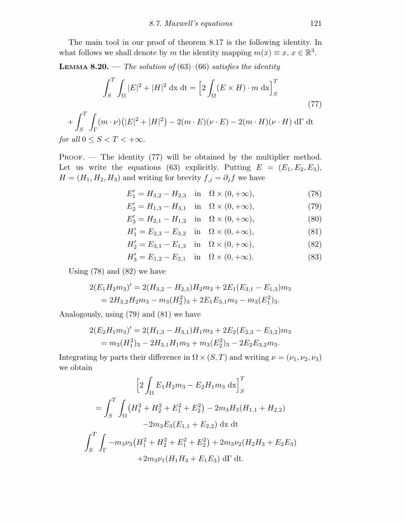
8.7. Maxwell’s equations 121
The main tool in our proof of theorem 8.17 is the following identity. In
what follows we shall denote by m the identity mapping m(x) ≡ x, x ∈ R3.
LEMMA 8.20. — The solution of (63)–(66) satisfies the identity
∫ T
S
∫
Ω
|E|2 + |H|2 dx dt =[2
∫
Ω
(E × H) · m dx]T
S
(77)
+
∫ T
S
∫
Γ
(m · ν)(|E|2 + |H|2
)− 2(m · E)(ν · E) − 2(m · H)(ν · H) dΓ dt
for all 0 ≤ S < T < +∞.
PROOF. — The identity (77) will be obtained by the multiplier method.
Let us write the equations (63) explicitly. Putting E = (E1, E2, E3),
H = (H1, H2, H3) and writing for brevity f,j = ∂jf we have
E′1 = H3,2 − H2,3 in Ω × (0,+∞), (78)
E′2 = H1,3 − H3,1 in Ω × (0,+∞), (79)
E′3 = H2,1 − H1,2 in Ω × (0,+∞), (80)
H ′1 = E2,3 − E3,2 in Ω × (0,+∞), (81)
H ′2 = E3,1 − E1,3 in Ω × (0,+∞), (82)
H ′3 = E1,2 − E2,1 in Ω × (0,+∞). (83)
Using (78) and (82) we have
2(E1H2m3)′ = 2(H3,2 − H2,3)H2m3 + 2E1(E3,1 − E1,3)m3
= 2H3,2H2m3 − m3(H22 )3 + 2E1E3,1m3 − m3(E
21)3.
Analogously, using (79) and (81) we have
2(E2H1m3)′ = 2(H1,3 − H3,1)H1m3 + 2E2(E2,3 − E3,2)m3
= m3(H21 )3 − 2H3,1H1m3 + m3(E
22)3 − 2E2E3,2m3.
Integrating by parts their difference in Ω× (S, T ) and writing ν = (ν1, ν2, ν3)
we obtain[2
∫
Ω
E1H2m3 − E2H1m3 dx]T
S
=
∫ T
S
∫
Ω
(H2
1 + H22 + E2
1 + E22
)− 2m3H3(H1,1 + H2,2)
−2m3E3(E1,1 + E2,2) dx dt∫ T
S
∫
Γ
−m3ν3
(H2
1 + H22 + E2
1 + E22
)+ 2m3ν2(H2H3 + E2E3)
+2m3ν1(H1H3 + E1E3) dΓ dt.
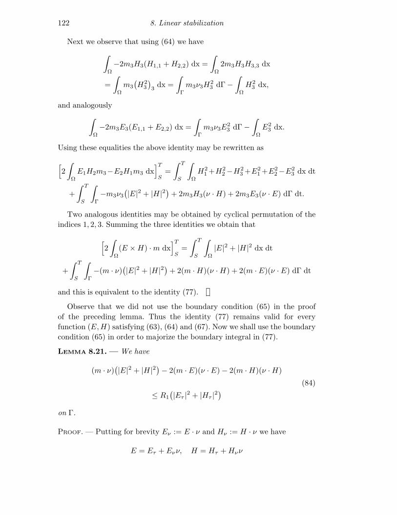
122 8. Linear stabilization
Next we observe that using (64) we have
∫
Ω
−2m3H3(H1,1 + H2,2) dx =
∫
Ω
2m3H3H3,3 dx
=
∫
Ω
m3
(H2
3
)3
dx =
∫
Γ
m3ν3H23 dΓ −
∫
Ω
H23 dx,
and analogously
∫
Ω
−2m3E3(E1,1 + E2,2) dx =
∫
Γ
m3ν3E23 dΓ −
∫
Ω
E23 dx.
Using these equalities the above identity may be rewritten as
[2
∫
Ω
E1H2m3−E2H1m3 dx]T
S=
∫ T
S
∫
Ω
H21 +H2
2 −H23 +E2
1 +E22 −E2
3 dx dt
+
∫ T
S
∫
Γ
−m3ν3
(|E|2 + |H|2
)+ 2m3H3(ν · H) + 2m3E3(ν · E) dΓ dt.
Two analogous identities may be obtained by cyclical permutation of the
indices 1, 2, 3. Summing the three identities we obtain that
[2
∫
Ω
(E × H) · m dx]T
S=
∫ T
S
∫
Ω
|E|2 + |H|2 dx dt
+
∫ T
S
∫
Γ
−(m · ν)(|E|2 + |H|2
)+ 2(m · H)(ν · H) + 2(m · E)(ν · E) dΓ dt
and this is equivalent to the identity (77).
Observe that we did not use the boundary condition (65) in the proof
of the preceding lemma. Thus the identity (77) remains valid for every
function (E,H) satisfying (63), (64) and (67). Now we shall use the boundary
condition (65) in order to majorize the boundary integral in (77).
LEMMA 8.21. — We have
(m · ν)(|E|2 + |H|2
)− 2(m · E)(ν · E) − 2(m · H)(ν · H)
(84)
≤ R1
(|Eτ |2 + |Hτ |2
)
on Γ.
PROOF. — Putting for brevity Eν := E · ν and Hν := H · ν we have
E = Eτ + Eνν, H = Hτ + Hνν
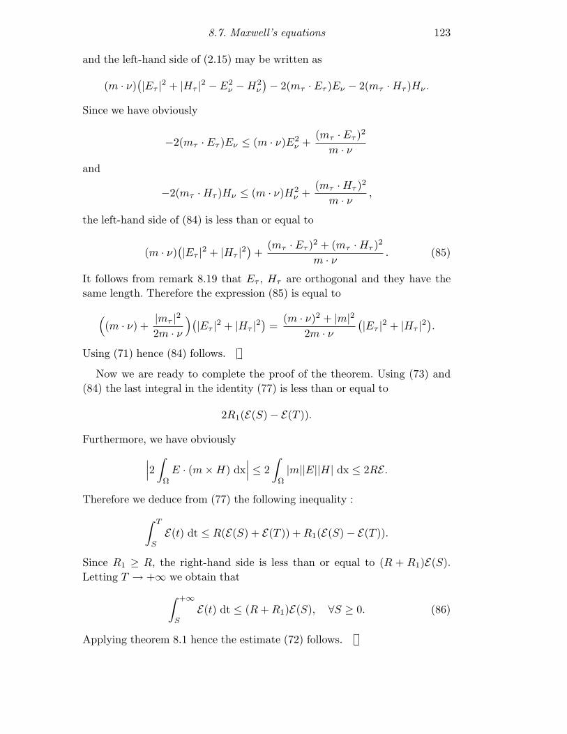
8.7. Maxwell’s equations 123
and the left-hand side of (2.15) may be written as
(m · ν)(|Eτ |2 + |Hτ |2 − E2
ν − H2ν
)− 2(mτ · Eτ )Eν − 2(mτ · Hτ )Hν .
Since we have obviously
−2(mτ · Eτ )Eν ≤ (m · ν)E2ν +
(mτ · Eτ )2
m · νand
−2(mτ · Hτ )Hν ≤ (m · ν)H2ν +
(mτ · Hτ )2
m · ν ,
the left-hand side of (84) is less than or equal to
(m · ν)(|Eτ |2 + |Hτ |2
)+
(mτ · Eτ )2 + (mτ · Hτ )2
m · ν . (85)
It follows from remark 8.19 that Eτ , Hτ are orthogonal and they have the
same length. Therefore the expression (85) is equal to
((m · ν) +
|mτ |22m · ν
)(|Eτ |2 + |Hτ |2
)=
(m · ν)2 + |m|22m · ν
(|Eτ |2 + |Hτ |2
).
Using (71) hence (84) follows.
Now we are ready to complete the proof of the theorem. Using (73) and
(84) the last integral in the identity (77) is less than or equal to
2R1(E(S) − E(T )).
Furthermore, we have obviously
∣∣∣2∫
Ω
E · (m × H) dx∣∣∣ ≤ 2
∫
Ω
|m||E||H| dx ≤ 2RE .
Therefore we deduce from (77) the following inequality :
∫ T
S
E(t) dt ≤ R(E(S) + E(T )) + R1(E(S) − E(T )).
Since R1 ≥ R, the right-hand side is less than or equal to (R + R1)E(S).
Letting T → +∞ we obtain that
∫ +∞
S
E(t) dt ≤ (R + R1)E(S), ∀S ≥ 0. (86)
Applying theorem 8.1 hence the estimate (72) follows.
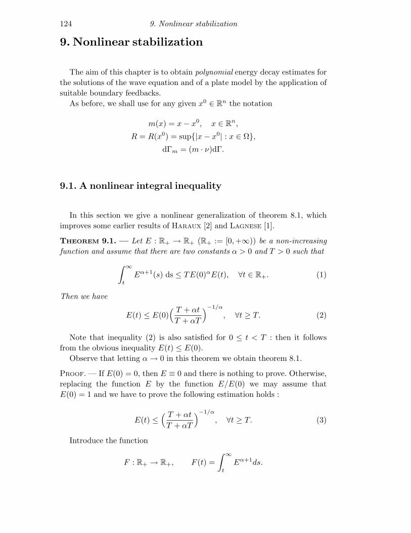
124 9. Nonlinear stabilization
9. Nonlinear stabilization
The aim of this chapter is to obtain polynomial energy decay estimates for
the solutions of the wave equation and of a plate model by the application of
suitable boundary feedbacks.
As before, we shall use for any given x0 ∈ Rn the notation
m(x) = x − x0, x ∈ Rn,
R = R(x0) = sup|x − x0| : x ∈ Ω,dΓm = (m · ν)dΓ.
9.1. A nonlinear integral inequality
In this section we give a nonlinear generalization of theorem 8.1, which
improves some earlier results of HARAUX [2] and LAGNESE [1].
THEOREM 9.1. — Let E : R+ → R+ (R+ := [0,+∞)) be a non-increasing
function and assume that there are two constants α > 0 and T > 0 such that
∫ ∞
t
Eα+1(s) ds ≤ TE(0)αE(t), ∀t ∈ R+. (1)
Then we have
E(t) ≤ E(0)( T + αt
T + αT
)−1/α
, ∀t ≥ T. (2)
Note that inequality (2) is also satisfied for 0 ≤ t < T : then it follows
from the obvious inequality E(t) ≤ E(0).
Observe that letting α → 0 in this theorem we obtain theorem 8.1.
PROOF. — If E(0) = 0, then E ≡ 0 and there is nothing to prove. Otherwise,
replacing the function E by the function E/E(0) we may assume that
E(0) = 1 and we have to prove the following estimation holds :
E(t) ≤( T + αt
T + αT
)−1/α
, ∀t ≥ T. (3)
Introduce the function
F : R+ → R+, F (t) =
∫ ∞
t
Eα+1ds.
9.1. A nonlinear integral inequality 125
It is non-increasing and locally absolutely continuous. Differentiating and
using (1) we find that
−F ′ ≥ T−α−1Fα+1 a.e. in (0,+∞),
whence
(F−α)′ ≥ αT−α−1 a.e. in (0, B), B := supt : E(t) > 0.
(Observe that F−α(t) is defined for t < B.) Integrating in [0, s] we obtain
that
(F (s)−α − F (0)−α) ≥ αT−α−1s for every s ∈ [0, B),
whence
F (s) ≤ (F (0)−α + αT−α−1s)−1/α for every s ∈ [0, B). (4)
Since F (s) = 0 if s ≥ B, this inequality holds in fact for every s ∈ R+. Since
F (0) ≤ TE(0)α+1 = T by (1), the right-hand side of (4) is less than equal to
(T−α + αT−α−1s)−1/α = T (α+1)/α(T + αs)−1/α.
On the other hand, E being nonnegative and non-increasing, the left-hand
side of (4) may be estimated as follows :
F (s) =
∫ +∞
s
Eα+1 dt ≥∫ T+(α+1)s
s
Eα+1 dt ≥ (T +αs)E(T +(α+1)s)α+1.
Therefore we deduce from (4) the estimate
(T + αs)E(T + (α + 1)s)α+1 ≤ T (α+1)/α(T + αs)−1/α,
whence
E(T + (α + 1)s) ≤(1 +
αs
T
)−1/α
, ∀s ≥ 0.
Choosing t := T + (α + 1)s hence the inequality (3) follows.
REMARK 9.2. — The theorem is optimal in the following sense : given
α > 0, T > 0, C > 0 and t′ ≥ T arbitrarily, there exists a non-increasing
function E : R+ → R+ satisfying (1) and such that
E(0) = C and E(t′) = E(0)(T + αt′
T + αT
)−1/α
.
126 9. Nonlinear stabilization
We leave to the reader to verify that the following example has these
properties :
E(t) :=
C(1 + αC−αt/T
)−1/α, if 0 ≤ t ≤ t′′
C(1 + α)1/α(1 + αC−αt′/T
)−1/α, if t′′ ≤ t ≤ t′
0, if t > t′
(5)
where t′′ = (t′−TCα)/(α+1). Let us also note that for t < T we cannot state
more than the trivial estimate E(t) ≤ E(0). Indeed, for any given α > 0,
T > 0, C > 0 and t′ < T the function
E(t) :=
C, if 0 ≤ t ≤ T
0, if t > T(6)
satisfies (1) and E(t′) = E(0) = C.
REMARK 9.3. — Assume that E is also continuous. Then the inequalities
(3) are strict ; in particular, E(T ) < E(0). See KOMORNIK [9], [12] for this
result, for a detailed study of integral inequalities of type (1) (also for α < 0)
and for the study of closely related differential inequalities.
9.2. Uniform stabilization of the wave equation I
Fix a point x0 ∈ Rn and consider the nonlinear problem
u′′ − ∆u = 0 in Ω × R+, (7)
u = 0 on Γ0 × R+, (8)
∂νu + (m · ν)g(u′) = 0 on Γ1 × R+, (9)
u(0) = u0 and u′(0) = u1 on Ω, (10)
a particular case of the problem in section 7.2.
We assume that g : R → R is a non-decreasing, continuous function
satisfying g(0) = 0 and we assume that
n ≥ 3, (11)
Γ0 6= ∅ and Γ0 ∩ Γ1 = ∅, (12)
m · ν ≤ 0 on Γ0 and m · ν ≥ 0 on Γ1. (13)
(More general situations are considered in ZUAZUA [5], CONRAD AND RAO [1]
and in KOMORNIK [10].)
9.2. Uniform stabilization of the wave equation I 127
We recall that the energy is defined by
E := 12
∫
Ω
|u′|2 + |∇u|2 dx.
In this section we prove the
THEOREM 9.4. — Assume (11)–(13). Assume that there exist p > 1 and
four constants c1, c2, c3, c4 > 0 such that
c1|x|p ≤ |g(x)| ≤ c2|x|1/p if |x| ≤ 1 (14)
and
c3|x| ≤ |g(x)| ≤ c4|x| if |x| > 1. (15)
Then for any given (u0, u1) ∈ H1Γ0
(Ω)×L2(Ω) the solution of (7)–(10) satisfies
the estimates
E(t) ≤ Ct2/(1−p), ∀t > 0 (16)
with a constant C only depending on the initial energy E(0) (and in a
continuous way).
Theorem 9.4 improves some earlier results of ZUAZUA [5] and CONRAD AND
RAO [1]. Let us note that the dependence of the constant C on E(0) was
studied in detail by CARPIO [1] and later by SOUPLET [1] and KOUEMOU [1].
REMARK 9.5. — A similar result holds for p = 1 : then (16) is replaced by
E(t) ≤ CE(0)e−ωt, ∀t > 0
with two positive constants C,ω, independent of the initial data. Thus we
may recover certain results of the preceding chapter.
First we shall prove the theorem under the additional hypothesis that
g is globally Lipschitz continuous.
This assumption will be removed at the end of this section.
By lemma 7.7 and by the inequality (7.19) in theorem 7.4 it is sufficient to
prove the estimate (16) for smooth initial data (u0, u1) ∈ D(A) : the general
case then follows by an obvious density argument.
In this case by theorem 7.5 the solution of (7)–(10) is sufficiently smooth
to justify all computations that follow.
We begin by generalizing lemma 8.4 :
128 9. Nonlinear stabilization
LEMMA 9.6. — The function E : R+ → R+ is non-increasing, locally
absolutely continuous and
E′ = −∫
Γ1
(m · ν)u′g(u′) dΓ a.e. in R+. (17)
PROOF. — Given 0 ≤ S < T < ∞ arbitrarily, we have
0 =
∫ T
S
∫
Ω
u′(u′′ − ∆u) dx dt
=
∫ T
S
∫
Ω
u′u′′ + ∇u · ∇u′ dx dt −∫ T
S
∫
Γ
u′∂νu dΓ dt
=
∫ T
S
∫
Ω
u′u′′ + ∇u · ∇u′ dx dt +
∫ T
S
∫
Γ1
(m · ν)u′g(u′) dΓ dt
whence
E(S) − E(T ) =
∫ T
S
∫
Γ1
(m · ν)u′g(u′) dΓ dt. (18)
Since m · ν ≥ 0 on Γ1 and xg(x) ≥ 0, ∀x ∈ R, the right-hand side of (18) is
nonnegative ; hence E is non-increasing. Furthermore, (18) implies that E is
locally absolutely continuous and that (17) is satisfied.
Next we generalize the identity of lemma 8.8 :
LEMMA 9.7. — Putting for brevity
Mu := 2m · ∇u + (n − 1)u, (19)
for any fixed 0 ≤ S < T < ∞ we have
2
∫ T
S
E(p+1)/2dt −∫ T
S
E(p−1)/2
∫
Γ0
(∂νu)2dΓm dt
=[E(p−1)/2
∫
Ω
u′Mudx]S
T+
p − 1
2
∫ T
S
E(p−3)/2E′
∫
Ω
u′Mudx dt (20)
+
∫ T
S
E(p−1)/2
∫
Γ1
(u′)2 − |∇u|2 − g(u′)MudΓm dt.
PROOF. — We have
0 =
∫ T
S
E(p−1)/2
∫
Ω
(Mu)(u′′ − ∆u) dx dt
=[E(p−1)/2
∫
Ω
u′Mu dx]T
S− p − 1
2
∫ T
S
E(p−3)/2E′
∫
Ω
u′Mu dx dt (21)
−∫ T
S
E(p−1)/2
∫
Ω
u′Mu′ + (Mu)(∆u) dx dt.
9.2. Uniform stabilization of the wave equation I 129
Integrating by parts and using the relation div m = n we transform the
interior integral in the last term as follows :
∫
Ω
u′Mu′ + (Mu)(∆u) dx
=
∫
Ω
m · ∇(u′)2 + (n − 1)(u′)2 −∇u · ∇(Mu) dx +
∫
Γ
(Mu)∂νu dΓ
=
∫
Ω
m · ∇(u′)2 + (n − 1)(u′)2 − 2|∇u|2 − m · ∇|∇u|2
−(n − 1)|∇u|2 dx +
∫
Γ
(Mu)∂νu dΓ
= −∫
Ω
(u′)2 + |∇u|2 dx +
∫
Γ
(m · ν)((u′)2 − |∇u|2) + (Mu)∂νu dΓ
= −∫
Ω
(u′)2 + |∇u|2 dx +
∫
Γ0
−(m · ν)|∇u|2 + (2m · ∇u)∂νu dΓ
+
∫
Γ1
(u′)2 − |∇u|2 − (Mu)g(u′) dΓm.
Since (8) implies that ∇u = ν∂νu on Γ0, hence we conclude that
∫
Ω
u′Mu′ + (Mu)(∆u) dx = −2E +
∫
Γ0
(∂νu)2 dΓm
+
∫
Γ1
(u′)2 − |∇u|2 − (Mu)g(u′) dΓm.
Substituting into (21) we obtain (20).
The following lemma is an immediate consequence of the definition of the
energy and of the hypothesis Γ0 6= ∅. Here and in the sequel c will denote
diverse positive constants only depending on E(0).
LEMMA 9.8. — We have
∣∣∣∫
Ω
u′Mu dx∣∣∣ ≤ cE. (22)
We deduce from lemma 9.8 and from the non-increasingness of the energy
that∣∣∣E(p−1)/2
∫
Ω
u′Mu dx∣∣∣ ≤ cE(p+1)/2 ≤ cE
and∣∣∣E(p−3)/2E′
∫
Ω
u′Mu dx∣∣∣ ≤ −cE(p−1)/2E′ ≤ −c
(E(p+1)/2
)′;
130 9. Nonlinear stabilization
hence the first and second terms on the right-hand side of the identity (20)
are majorized by cE(S). Since the second integral on the left-hand side of
(20) is ≤ by (12), we deduce from (20) that
2
∫ T
S
E(p+1)/2 dt ≤ cE(S)+
∫ T
S
E(p−1)/2
∫
Γ1
(u′)2−|∇u|2−g(u′)Mu dΓm dt;
Using the definition of Mu and the relation |m| ≤ R, we obtain for any fixed
ε > 0 the inequality
2
∫ T
S
E(p+1)/2 dt ≤ cE(S)
+
∫ T
S
E(p−1)/2
∫
Γ1
(u′)2 + R2g(u′)2 + εu2 +(n − 1)2
4εg(u′)2 dΓm dt.
Choosing ε = ε(Ω) such that
ε
∫
Γ1
u2 dΓm ≤ 12
∫
Ω
|∇u|2 dx (≤ E),
hence we conclude that
∫ T
S
E(p+1)/2dt ≤ cE(S) + c
∫ T
S
E(p−1)/2
∫
Γ1
(u′)2 + g(u′)2 dΓm dt. (23).
We are going to majorize the last integral in (23). Set
Γ2 = x ∈ Γ1 : |u′(x)| ≤ 1 and Γ3 = x ∈ Γ1 : |u′(x)| > 1. (24)
(Note that Γ2 and Γ3 depend on t ∈ R+.) Using (15) and (17) we obtain that
∫ T
S
E(p−1)/2
∫
Γ3
(u′)2 + g(u′)2 dΓm dt
(25)
≤ −c
∫ T
S
E(p−1)/2E′ dt ≤ cE(p+1)/2(S) ≤ cE(S).
Furthermore, using (14) we also have
∫
Γ2
(u′)2 + g(u′)2 dΓm ≤ c
∫
Γ2
(u′g(u′))2/(p+1) dΓm
≤ c( ∫
Γ2
u′g(u′) dΓm
)2/(p+1)
≤ c(−E′)2/(p+1);
9.2. Uniform stabilization of the wave equation I 131
hence, using the Young inequality we obtain for every ε > 0 the estimate
∫ T
S
E(p−1)/2
∫
Γ2
(u′)2 + g(u′)2 dΓm dt
≤ c
∫ T
S
E(p−1)/2(−E′)2/(p+1) dt (26)
≤∫ T
S
εE(p+1)/2 − c(ε)E′ dt ≤ ε
∫ T
S
E(p+1)/2 dt + c(ε)E(S).
Combining (23), (25) and (26) we find that
∫ T
S
E(p+1)/2 dt ≤ c(ε)E(S) + εc
∫ T
S
E(p+1)/2 dt.
Choosing ε such that εc < 1, hence we conclude that
∫ T
S
E(p+1)/2 dt ≤ cE(S). (27)
Letting T → +∞ we obtain that
∫ ∞
S
E(p+1)/2 dt ≤ cE(S), ∀S ≥ 0,
and we conclude by applying theorem 9.1 with α = (p − 1)/2 and
T = cE(0)−α.
Thus the proof of the theorem is completed in the case of globally Lipschitz
continuous functions g. Turning to the general case, let us admit for a moment
the following
LEMMA 9.9. — Let g : R → R be a non-decreasing, continuous function
satisfying the inequalities (14) and (15) for some p ≥ 1 and for some positive
constants ci. Then there exists a sequence of non-decreasing, globally Lipschitz
continuous functions gk : R → R satisfying the inequalities
c′1|x|p ≤ |gk(x)| ≤ c′2|x|1/p if |x| ≤ 1 (28)
and
c′3|x| ≤ |gk(x)| ≤ c′4|x| if |x| > 1. (29)
with suitable positive constants c′i, independent of k, and such that
|gk(x)| ≤ |g(x)|, ∀x ∈ R, k = 1, 2, . . . , (30)
132 9. Nonlinear stabilization
and
gk(x) → g(x), ∀x ∈ R, (31)
If we replace the function g in the equation (9) by one of the functions
gk, the already proved part of the theorem applies. Using theorem 7.3 the
general case of the theorem will follow if we prove that
(I + Ak)−1W → (I + A)−1W in H, ∀W ∈ H (32)
where Ak denotes the generator of the semigroup associated with the problem
(7)–(10) where g is replaced by gk. Putting f = W2 − AW1 and denoting by
u, uk the solutions of
(I + A + B)u = f and (I + A + Bk)uk = f
where we use the same notations as in the proof of proposition 7.6 (and Bk
denotes the operator analogous to B but corresponding to the function gk),
it is sufficient to prove that uk → u in H as k → +∞.
We have
〈(I + A + Bk)uk − (I + A + Bk)u, uk − u〉V ′,V = 〈(B − Bk)u, uk − u〉V ′,V
whence
‖uk − u‖2V ≤ ‖(B − Bk)u‖V ′‖uk − u‖V
and therefore
‖uk − u‖V ≤ ‖g(u) − gk(u)‖L(2n−2)/n(Γ1).
By (28) and (29) the expression on the right-hand side tends to zero by
Lebesgue’s dominated convergence theorem. Hence uk → u in V and therefore
also in H. Since
(I + Ak)−1W = (uk + W1, uk) and (I + A)−1W = (u + W1, u),
hence (32) follows.
PROOF OF LEMMA 9.9. — Set
gk(x) := g((idR + k−1g)−1(x)
), x ∈ R, k = 1, 2, . . . .
One may readily verify that the functions gk are well-defined, continuous,
non-decreasing and that properties (30), (31) are satisfied. It follows from
9.3. Uniform stabilization of the wave equation II 133
(14), (15) and (30) that the right-hand side inequalities in (28), (29) are
satisfied with c′2 = c2 and c′4 = c4.
To prove their Lipschitz continuity choose x1, x2 ∈ R arbitrarily and set
yi := (idR + k−1g)−1(xi), i = 1, 2.
Then we have gk(xi) = g(yi) and therefore
x1 − x2 = (y1 − y2) + k−1(gk(x1) − gk(x2)
).
Using the monotonicity of g hence we conclude that
|gk(x1) − gk(x2)| ≤ k|x1 − x2|.
To prove the first inequality in (28) fix 0 ≤ x ≤ 1 arbitrarily (the case
−1 ≤ x ≤ 0 is similar) and set y := (idR +k−1g)−1(x). Then y +k−1g(y) = x
and 0 ≤ y ≤ x. If y ≥ x/2, then
gk(x) = g(y) ≥ g(x/2) ≥ c1(x/2)p.
If y < x/2, then k−1g(y) ≥ x/2 and therefore
gk(x) = g(y) ≥ x/2 ≥ (x/2)p.
Hence the first inequality in (28) is satisfied with c′1 := 2−p minc1, 1.To prove the first inequality in (29) let us choose a number 0 < ε ≤ 1/2
such that ε + g(ε) < 1 and −ε + g(−ε) > −1. Observe that (14) and (15)
imply the existence of a positive constant c′′3 such that
|g(y)| ≥ c′′3 |y| if |y| ≥ ε.
Now fix x ≥ 1 arbitrarily (the case x ≤ −1 is analogous) and set
y := (idR + k−1g)−1(x) as above. We have y + k−1g(y) = x and ε ≤ y ≤ x. If
y ≥ x/2, then
gk(x) = g(y) ≥ g(x/2) ≥ (c′′3/2)x
because x/2 ≥ 1/2 ≥ ε. If y < x/2, then k−1g(y) ≥ x/2 and therefore
gk(x) = g(y) ≥ x/2.
Hence the first inequality in (29) is satisfied with c′3 := 2−1 minc′′3 , 1.
134 9. Nonlinear stabilization
9.3. Uniform stabilization of the wave equation II
The theorem 9.4 proved in the preceding section has a serious drawback :
it never applies for bounded functions g (because of c3 > 0 in (15)). The
purpose of this section is to obtain a variant of this theorem for bounded
feedback functions.
THEOREM 9.10. — Assume (11)–(13) and assume that the function g is
bounded, globally Lipschitz continuous and that the inequalities (14) are
satisfied with some positive constants c1, c2 and with a number p satisfying
p ≥ n − 1. (30)
Then for every
(u0, u1) ∈(H2(Ω) ∩ H1
Γ0(Ω)
)× H1
Γ0(Ω) (31)
satisfying
∂u0
∂ν+ (m · ν)g(u1) = 0 on Γ1, (32)
the solution of (7)-(10) satisfies the estimates
E(t) ≤ Ct2/(1−p), ∀t > 0 (33)
with a constant C depending on the initial data.
REMARK 9.11. — Observe that if the condition (30) is not satisfied initially,
it will be satisfied if we replace p by n − 1 ; at the same time (14) continues
to hold with the same constants c1, c2.
PROOF. — Repeating the proof of the preceding theorem, except that part
where the first inequality of (15) involving c3 is applied, now we obtain the
following inequality :
∫ T
S
E(p+1)/2 dt ≤ cE(S) + c
∫ T
S
E(p−1)/2
∫
Γ3
(u′)2 dΓm dt. (34)
It remains to establish the estimate
E(p−1)/2
∫
Γ3
(u′)2 dΓm ≤ εE(p+1)/2 − c(ε)E′ (35)
9.4. Uniform stabilization of Kirchhoff plates 135
for every ε > 0. Then the theorem will follow. Indeed, choosing a sufficiently
small ε, (34)–(35) imply (27) and the proof may be completed by applying
theorem 9.1 as in the preceding section.
For brevity we shall denote the norm of Lβ(Γ) by ‖ ‖β . Set
s := 2/(p + 1) and α := (2 − s)/(1 − s);
we have 0 < s < 1 and α = 2p/(p − 1) > 2. We establish for every ε > 0 the
inequality
E(p−1)/2
∫
Γ3
(u′)2 dΓm ≤ εE(p+1)/2‖u′‖αα − c(ε)E′. (36)
Indeed, we have
E(p−1)/2
∫
Γ3
(u′)2 dΓm ≤ cE(p−1)/2
∫
Γ3
|u′|2−s(u′g(u′))s dΓm
≤ cE(p−1)/2‖|u′|2−s‖1/(1−s)‖(u′g(u′))s‖1/s
= cE(p−1)/2‖u′‖(1−s)αα ‖u′g(u′)‖s
1
= cE(p−1)/2‖u′‖(1−s)αα (−E′)s ≤ εE(p−1)/(2(1−s))‖u′‖α
α − c(ε)E′
= εE(p+1)/2‖u′‖αα − c(ε)E′.
Using the trace theorem
H1(Ω) → L2p/(p−1)(Γ) = Lα(Γ)
(following from (30)) and the regularity property (7.24) we deduce from (36)
that
E(p−1)/2
∫
Γ3
(u′)2 dΓm ≤ cεE(p+1)/2 − c(ε)E′;
hence (35) follows (with another ε).
9.4. Uniform stabilization of Kirchhoff plates
Consider the problem of section 7.3 :
u′′ + ∆2u = 0 in Ω × R+, (37)
u = uν = 0 on Γ0 × R+, (38)
uνν + µuττ = 0 on Γ1 × R+, (39)
uννν + (2 − µ)uττν = (m · ν)g(u′) on Γ1 × R+, (40)
u(0) = u0 and u′(0) = u1 on Ω. (41)
136 9. Nonlinear stabilization
Assume that there is a point X0 ∈ R2 such that
m · ν ≥ 0 on Γ1 and m · ν ≤ 0 on Γ0. (42)
We shall prove the
THEOREM 9.12. — Assume (42) and assume that there exist two numbers
p, q > 1 and two positive constants c1, c2 such that
c1|x|p ≤ |g(x)| ≤ c2|x|1/p if |x| ≤ 1 (43)
and
c1|x| ≤ |g(x)| ≤ c2|x|q if |x| > 1. (44)
Then for any given (u0, u1) ∈ H2Γ0
× L2(Ω) the solution of (37)–(40) satisfies
the estimates
E(t) ≤ Ct2/(1−p), ∀t > 0 (45)
with a constant C only depending on the initial energy E(0) (and in a
continuous way).
REMARK 9.13. — A similar result holds for p = 1 : then the estimate (45)
is replaced by
E(t) ≤ Ce−ωt, ∀t > 0
with two positive constants C,ω which do not depend on the initial data.
REMARK 9.14. — Theorem 9.12 improves some earlier results of LAGNESE
[2] (whose method is followed here) and of RAO [1] by weakening their growth
assumptions and by using one feedback only. Also see KOMORNIK [11] for a
more general result.
There are many other theorems concerning the strong or uniform
stabilization of different plate and beam models ; see e.g. BARTOLOMEO
AND TRIGGIANI [1], HORN [1], HORN AND I. LASIECKA [1], LAGNESE [2],
LAGNESE AND LEUGERING [1], I. LASIECKA [1], [2], LASIECKA AND TATARU
[1], LASIECKA AND TRIGGIANI [3], LEBEAU [1], W. LITTMANN AND L. MARKUS
[1], LITTMANN AND TAYLOR [1], PUEL AND TUCSNAK [1], TATARU [1].
The rest of this section is devoted to the proof of theorem 9.12. Using
lemma 9.9 and the argument following it in section 9.2 we may assume
without loss of generality that g is globally Lipschitz. Furthermore, using
theorem 7.9 and a density argument we may assume that the solutions verify
9.4. Uniform stabilization of Kirchhoff plates 137
the regularity conditions (7.53) and (7.54) ; then all computations that follow
are justified.
LEMMA 9.15. — The function E : R+ → R+ is non-increasing, locally
absolutely continuous and
E′ = −∫
Γ1
u′g(u′) dΓm a.e. on R+. (46)
PROOF. — Given 0 ≤ S < T < +∞ arbitrarily, we apply lemma 7.12 ; we
obtain that
0 =
∫ T
S
∫
Ω
u′(u′′ + ∆2u) dX dt =
∫ T
S
∫
Ω
u′u′′ + Q(u, u′) dX dt
+
∫ T
S
∫
Γ
(uνν + (2 − µ)uττ )νu′ − (uνν + µuττ )u′ν dΓ dt
=[ 1
2
∫
Ω
(u′)2 + Q(u) dX]T
S+
∫ T
S
∫
Γ1
(m · ν)u′g(u′) dΓ dt
=[ 1
2
∫
Ω
(u′)2 + Q(u) dX]T
S+
∫ T
S
∫
Γ1
(m · ν)u′g(u′) dΓ dt,
i.e.
E(S) − E(T ) =
∫ T
S
∫
Γ1
u′g(u′) dΓm dt. (47)
This implies that E is locally absolutely continuous ; differentiating (47) we
find (46). Finally, E is non-increasing because the right-hand side of (47) is
nonnegative by the increasingness of g and by hypothesis (42).
LEMMA 9.16. — Given v ∈ H3(Ω) arbitrarily, the following identity holds
true : ∫
Ω
Q(v,m · ∇v) dX =
∫
Ω
Q(v) dX + 12
∫
Γ
Q(v) dΓm. (48)
PROOF. — Integrating by parts we obtain the following five simple identities :∫
Ω
vxx(m1vx + m2vy)xx dX =
∫
Ω
2v2xx + m1vxxvxxx + m2vxxvxxy dX
=
∫
Ω
2v2xx + 1
2m · ∇(v2xx) dX,
∫
Ω
vyy(m1vx + m2vy)yy dX =
∫
Ω
2v2yy + m1vyyvyyx + m2vyyvyyy dX
=
∫
Ω
2v2yy + 1
2m · ∇(v2yy) dX,
138 9. Nonlinear stabilization
∫
Ω
vxx(m1vx + m2vy)yy dX =
∫
Ω
2vxxvyy + m1vxxvxyy + m2vxxvyyy dX,
∫
Ω
vyy(m1vx + m2vy)xx dX =
∫
Ω
2vxxvyy + m1vyyvxxx + m2vyyvyxx dX,
∫
Ω
vxy(m1vx + m2vy)xy dX =
∫
Ω
2v2xy + m1vxyvxxy + m2vxyvxyy dX
=
∫
Ω
2v2xy + 1
2m · ∇(v2xy) dX.
Combining these identities, using the definitions of Q(v), Q(u, v) and
finally applying the divergence theorem we obtain that
∫
Ω
Q(v,m · ∇v) dX =
∫
Ω
2Q(v) + 12m · ∇Q(v) dX =
∫
Ω
(2− 1
2divm)Q(v) dX
+12
∫
Γ
(m · ν)Q(v) dΓ =
∫
Ω
Q(v) dX + 12
∫
Γ
Q(v) dΓm.
Now we prove our basic identity :
LEMMA 9.17. — Given 0 ≤ S < T < +∞ arbitrarily, the following identity
holds true :
4
∫ T
S
E(p+1)/2 dt −∫ T
S
E(p−1)/2
∫
Γ0
(∆u)2 dΓm dt
=[E(p−1)/2
∫
Ω
2u′m · ∇u dX]S
T
(49)
+(p − 1)
∫ T
S
E(p−3)/2E′
∫
Ω
u′m · ∇u dX dt
+
∫ T
S
E(p−1)/2
∫
Γ1
(u′)2 − Q(u) − 2(m · ∇u)g(u′) dΓm dt.
PROOF. — We multiply the equation (39) by 2E(p−1)/2m·∇u and we integrate
by parts in Ω × (S, T ). Using lemmas 7.12 and 9.16 we obtain that
0 =
∫ T
S
E(p−1)/2
∫
Ω
2m · ∇u(u′′ + ∆2u) dX dt
=[E(p−1)/2
∫
Ω
2u′m · ∇u dX]T
S− (p − 1)
∫ T
S
E(p−3)/2E′
∫
Ω
u′m · ∇udXdt
9.4. Uniform stabilization of Kirchhoff plates 139
+
∫ T
S
E(p−1)/2
∫
Ω
−2u′m · ∇u′ + 2Q(u,m · ∇u) dX dt
+2
∫ T
S
E(p−1)/2
∫
Γ
(uνν + (2−µ)uττ )νm · ∇u− (uνν + µuττ )(m · ∇u)ν dΓ dt
=[E(p−1)/2
∫
Ω
2u′m · ∇u dX]T
S− (p − 1)
∫ T
S
E(p−3)/2E′
∫
Ω
u′m · ∇u dX dt
+
∫ T
S
E(p−1)/2
∫
Ω
−m · ∇(u′)2 + 2Q(u) dX dt
+
∫ T
S
E(p−1)/2
∫
Γ
(m · ν)Q(u) + 2(uνν + (2 − µ)uττ )νm · ∇u
−2(uνν + µuττ )(m · ∇u)ν dΓ dt
=[E(p−1)/2
∫
Ω
2u′m · ∇u dX]T
S− (p − 1)
∫ T
S
E(p−3)/2E′
∫
Ω
u′m · ∇u dX dt
+2
∫ T
S
E(p−1)/2
∫
Ω
(u′)2 + Q(u) dX dt
+
∫ T
S
E(p−1)/2
∫
Γ
(m · ν)(Q(u) − (u′)2) + 2(uνν + (2 − µ)uττ )νm · ∇u
−2(uνν + µuττ )(m · ∇u)ν dΓ dt.
Recalling the definition of the energy we conclude that
4
∫ T
S
E(p+1)/2 dt
=[E(p−1)/2
∫
Ω
2u′m · ∇u dX]S
T+ (p − 1)
∫ T
S
E(p−3)/2E′
∫
Ω
u′m · ∇u dX dt
+
∫ T
S
E(p−1)/2
∫
Γ
(m · ν)((u′)2 − Q(u)) − 2(uνν + (2 − µ)uττ )νm · ∇u
+2(uνν + µuττ )(m · ∇u)ν dΓ dt.
It remains to show that
(m · ν)((u′)2 − Q(u)) − 2(uνν + (2 − µ)uττ )νm · ∇u
+2(uνν + µuττ )(m · ∇u)ν = (m · ν)(u′)2 − Q(u) − 2(m · ∇u)(αu + g(u′))
on Γ1 and
(m · ν)((u′)2 − Q(u)) − 2(uνν + (2 − µ)uττ )νm · ∇u
+2(uνν + µuττ )(m · ∇u)ν = (∆u)2 (50)
on Γ0.
140 9. Nonlinear stabilization
The first equality follows at once from the boundary conditions (39) and
(40).
For the proof of (50) first observe that the boundary conditions (38) imply
u′ = ux = uy = 0 on Γ0. Consequently, the vectors ∇ux = (uxx, uxy) and
∇uy = (uxy, uyy) are orthogonal to Γ0 and therefore they are parallel. Hence
uxxuyy = u2xy and Q(u) = (∆u)2 on Γ0. Furthermore, m ·∇u = (m ·ν)uν and
(m · ∇u)ν = (m1ux + m2uy)ν = (m · ν)uνν + (m · τ)uντ = (m · ν)uνν
on Γ0 because uν = 0 on Γ0.
Combining these relations we conclude that the left-hand side of (50) is
equal to
−(m · ν)(∆u)2 + 2(m · ν)u2νν .
Since the boundary conditions (38) imply that uττ = 0 on Γ0, we have
−(m · ν)(∆u)2 + 2(m · ν)u2νν = (m · ν)(∆u)2.
This completes the proof of (50) and that of the lemma.
In order to majorize the right-hand side of (49) we need the
LEMMA 9.18. — The semi-norm p : H2(Ω) → R+ defined by
p(v) :=(∫
Ω
v2xx + v2
xy + v2yy dX
)1/2
(51)
is equivalent to the norm || ||H2(Ω) on the subspace H2Γ0
(Ω).
PROOF. — First we show that p is a norm on H2Γ0
(Ω). Indeed, let v ∈ H2Γ0
(Ω)
such that p(v) = 0. Then the second derivative of v vanishes. Since Ω is
connexe, hence we conclude that v is affine. Since Γ0 6= ∅ and v = vx = vy = 0
on Γ0 by hypotheses Γ0 6= ∅ and (40), it follows that v = 0.
The estimate
p ≤ c|| ||H2(Ω) (52)
is obvious. Assume that the inverse inequality is false. Then there exists a
sequence vk in H2Γ0
(Ω) such that
||vk||H2(Ω) = 1, k = 1, 2, . . . (53)
and
p(vk) → 0. (54)
9.4. Uniform stabilization of Kirchhoff plates 141
By the compactness of the imbedding H2(Ω) ⊂ H1(Ω) we may assume, by
extracting a subsequence if needed, that
vk → v in H1(Ω)
for some v ∈ H1(Ω). Using (51) and (54) we conclude that
vk → v in H2(Ω);
consequently, using (52) and (54) we obtain that v = 0 and hence
vk → 0 in H2(Ω).
But this contradicts (53).
In what follows c will denote diverse positive constants depending on E(0)
only.
COROLLARY 9.19. — We have
∣∣∣∫
Ω
u′m · ∇u dX∣∣∣ ≤ cE. (55)
PROOF. — Using the trivial inequality
∣∣∣∫
Ω
u′m · ∇u dX∣∣∣ ≤ c
(||u′||2L2(Ω) + ||u||2H1(Ω)
)
and the definition of the energy, (55) follows from the preceding lemma and
from the hypothesis 0 < µ < 1.
LEMMA 9.20. — Given 0 ≤ S < T < +∞ arbitrarily, we have
∫ T
S
E(p+1)/2 dt ≤ cE(p+1)/2(S)
(56)
+c
∫ T
S
E(p−1)/2
∫
Γ1
(u′)2 + |∇u||g(u′)| dΓm dt.
PROOF. — Since m · ν ≤ 0 on Γ0, the left-hand side of (49) is minorized by
its first term. Applying corollary 9.19 and using the non-increasingness of E
we may estimate the first and second term on the right-hand side of (49) as
follows :
[E(p−1)/2
∫
Ω
2u′m · ∇u dX]S
T+ (p − 1)
∫ T
S
E(p−3)/2E′
∫
Ω
u′m · ∇u dX dt
≤ cE(p+1)/2(S) + cE(p+1)/2(T ) − c
∫ T
S
E(p−1)/2E′ dt ≤ cE(p+1)/2(S).
142 9. Nonlinear stabilization
Furthermore, using hypothesis 0 < µ < 1 we have
Q(u) = µ(uxx + uyy)2 + (1 − µ)(u2xx + u2
yy + 2u2xy) ≥ 0
and therefore we deduce from (49) that
4
∫ T
S
E(p+1)/2 dt ≤ cE(p+1)/2(S)
+
∫ T
S
E(p−1)/2
∫
Γ1
(u′)2 − 2(m · ∇u)g(u′) dΓm dt
which implies (56).
Now we introduce the notation
Γ2 = x ∈ Γ1 : |u′(x)| ≤ 1 and Γ3 = x ∈ Γ1 : |u′(x)| > 1.
LEMMA 9.21. — Given 0 ≤ S < T < +∞ arbitrarily, we have
∫ T
S
E(p+1)/2 dt ≤ cE(p+1)/2(S)
+c
∫ T
S
E(p−1)/2
∫
Γ2
(u′)2 + |g(u′)|2 dΓm dt (57)
+c
∫ T
S
E(p−1)/2
∫
Γ3
(u′)2 + |g(u′)|1+q−1
dΓm dt.
PROOF. — For any fixed ε > 0 we deduce from (56) that
∫ T
S
E(p+1)/2 dt ≤ cE(p+1)/2(S)
+c
∫ T
S
E(p−1)/2
∫
Γ1
(u′)2 + ε|∇u|2 + c(ε)|g(u′)|2 dΓm dt (58)
+c
∫ T
S
E(p−1)/2
∫
Γ2
(u′)2 + ε|∇u|2 + ε|∇u|1+q + c(ε)|g(u′)|1+q−1
dΓm dt.
Using the Sobolev inequality
||u||W 1,γ(Γ) ≤ cE1/2, ∀γ ≥ 1
with γ = 2 and γ = 1 + q, we conclude from (58) that
∫ T
S
E(p+1)/2 dt ≤ cE(p+1)/2(S) + cε
∫ T
S
E(p+1)/2 dt
+c
∫ T
S
E(p−1)/2
∫
Γ2
(u′)2 + c(ε)|g(u′)|2 dΓm dt
+c
∫ T
S
E(p−1)/2
∫
Γ3
(u′)2 + c(ε)|g(u′)|1+q−1
dΓm dt.
9.4. Uniform stabilization of Kirchhoff plates 143
The lemma follows if we choose ε > 0 such that cε < 1.
Now we are ready to complete the proof of the theorem. Applying (43)
and (44) we have
∫
Γ2
|g(u′)|2 + (u′)2 dΓ ≤ c
∫
Γ2
(u′g(u′))2/(p+1) dΓ
≤ c(∫
Γ2
u′g(u′) dΓ)2/(p+1)
≤ c(−E′)2/(p+1)
and ∫
Γ3
|g(u′)|1+q−1
+ (u′)2 dΓ ≤ c
∫
Γ3
u′g(u′) dΓ ≤ −cE′.
Substituting into (57) we obtain for every ε > 0 the estimate
∫ T
S
E(p+1)/2 dt ≤ cE(p+1)/2(S)
+c
∫ T
S
E(p−1)/2(−E′)2/(p+1) dt − c
∫ T
S
E(p−1)/2E′ dt
≤ cE(p+1)/2(S) +
∫ T
S
εE(p+1)/2 − c(ε)E′ dt
≤ c(ε)E(S) + ε
∫ T
S
E(p+1)/2 dt.
Choosing ε < 1 we conclude that E satisfies an inequality of the form
∫ T
S
E(p+1)/2 dt ≤ AE(S) for every 0 ≤ S < T < +∞
with a suitable positive constant A. We may conclude by applying theorem
9.1.
144 10. Stabilization of the KdV equation
10.Stabilizationof theKorteweg–deVries equa-tion
In this chapter we shall study, following KOMORNIK, RUSSELL AND ZHANG
[1], [2] the stabilizability of the non-linear Korteweg–de Vries equation by
linear distributed feedbacks. The proof is based on a remarkable property
of this equation : the existence of an infinite sequence of conservation laws
corresponding to an infinite sequence of useful multipliers.
10.1. Formulation of the results
Let Ω = (0, 1), k > 0 and consider the problem
u′ + uux + uxxx = −k(u − [u]) in Ω × R+, (1)
u(0, t) = u(1, t), ∀t ∈ R+, (2)
ux(0, t) = ux(1, t), ∀t ∈ R+, (3)
uxx(0, t) = uxx(1, t), ∀t ∈ R+, (4)
u(0) = u0 on Ω (5)
where [u] denotes the mean-value of u defined by
[u] :=
∫
Ω
u dx. (6)
For k = 0 the equation (1) is a good model of shallow water : u(x, t)
denotes the depth of water at a point x at time t ; see MIURA [1], TEMAM [1].
The periodic boundary conditions correspond to a circular movement. In this
model [u] denotes the total volume of water.
For k > 0 the action of the ”feedback” −k(u − [u]) consists in balancing
the level of water, conserving at the same time its total volume. Indeed, the
latter property follows, at least formally, from (1), (2) and (5) :
[u]′ =
∫
Ω
u′ dx = −∫
Ω
uux + uxxx + k(u − [u]) dx
= −∫
Ω
(u2/2 + uxx)x dx + k[u] − k
∫
Ω
u dx
= −∫
Ω
(u2/2 + uxx)x dx = [u2/2 + uxx]10 = 0
10.1. Formulation of the results 145
whence
[u(t)] = [u0], ∀t ∈ R+. (7)
The following formal computation shows that u(t) converges exponentially
to the constant M := [u0] = [u] in L2(Ω) as t → +∞ :
(∫(u − [u])2 dx
)′
=
∫2(u − M)u′ dx
=
∫−2(u − M)(uux + uxxx + k(u − M)) dx
=
∫−2u2ux + 2Muux − 2uuxxx − 2k(u − M)2 dx
=[−(2/3)u3 + Mu2 − 2uuxx + u2
x
]10− 2k
∫(u − M)2 dx
= −2k
∫(u − M)2 dx
whence
‖u(t) − [u0]‖L2(Ω) = ‖u0 − [u0]‖L2(Ω)e−kt, ∀t ≥ 0. (8)
Let us introduce the Hilbert spaces
Hmp := w ∈ Hm(Ω) : wj(0) = wj(1), j = 0, . . . ,m − 1, m = 1, 2, . . .
H0p := L2(Ω) and H−1
p := (H1p )′.
Identifying (L2(Ω))′ with L2(Ω) we obtain the algebraical and topological
inclusions
· · · ⊂ H2p ⊂ H1
p ⊂ H0p ⊂ H−1
p .
The problem (1)–(5) is well-posed in the following sense :
THEOREM 10.1. — Let m ≥ 2 and u0 ∈ Hmp . Then the problem (1)–(5) has
a unique solution
u ∈ C(R+;Hmp ) ∩ C1(R+;Hm−3
p ). (9)
Furthermore, the mapping u0 7→ (u, u′) is continuous from Hmp into
Hm × Hm−3.
The solution u(t) converges quickly to the constant [u0] as t → +∞ :
146 10. Stabilization of the KdV equation
THEOREM 10.2. — Let m ≥ 2 and u0 ∈ Hmp . Then for every fixed k′ ∈]0, k[
there exists a constant C = C(u0, k′) such that the solution of (1)–(5) satisfies
the estimate
‖(u(t) − [u0], u′(t))‖Hmp ×Hm−3
p≤ Ce−k′t, ∀t ∈ R+. (10)
Theorems 10.1 et 10.2 were proved in KOMORNIK, RUSSELL AND ZHANG
[2]. Here we admit theorem 10.1 without proof and we only prove theorem
10.2 in the particular case m = 2.
10.2. Uniform stabilization by linear feedbacks
We shall often use the equality (7) and therefore we shall write [u] instead
of [u0]. For brevity we shall write∫
instead of∫Ω.
Applying a usual density argument it is sufficient to prove the estimates
(10) for u0 ∈ H5p . According to theorem 10.1 thus we may assume that
u ∈ C(R+;H5p ) ∩ C1(R+;H2
p ). (11)
This regularity property is sufficient to justify all computations which follow.
It is convenient to introduce the notations
M := [u0], v := u − M, v0 := u0 − M ; (12)
then we deduce from (1), (5), (7) and (11) that
v ∈ C(R+;H5p ), (13)
v ∈ C1(R+;H2p ), (14)
[v(t)] = 0, ∀t ∈ R+, (15)
v′ + vvx + Mvx + vxxx + kv = 0 in Ω × R+, (16)
v(0) = v0 on Ω, (17)
and the estimates (10) take the following form :
‖(v(t), v′(t))‖H2p×H−1
p≤ Ce−k′t, ∀t ∈ R+. (18)
LEMMA 10.3. — The function
t 7→∫
v(t)2 dx, t ∈ R+ (19)
10.2. Uniform stabilization by linear feedbacks 147
is continuously differentiable and
(∫v2 dx
)′
≡ −2k
∫v2 dx. (20)
PROOF. — Since H2p is a Banach algebra, it follows from (14) that the
function v2 is continuously differentiable. Hence the function (19), being the
composition of two function of class C2, is also continuously differentiable.
Using (16) and the periodicity of v (cf. (13)) we easily obtain the identity
(20) :
(∫v2 dx
)′
=
∫2vv′ dx =
∫−2v(vvx + Mvx + vxxx + kv) dx
=
∫−2v2vx − 2Mvvx − 2vvxxx − 2kv2 dx
=[−(2/3)v3 − Mv2 − 2vvxx + v2
x
]10− 2k
∫v2 dx = −2k
∫v2 dx.
LEMMA 10.4. — The function
t 7→∫
vx(t)2 − (1/3)v3(t)2 dx, t ∈ R+ (21)
is continuously differentiable and
(∫vx(t)2 − (1/3)v3(t)2 dx
)′
≡ −2k
∫vx(t)2 − (1/2)v3(t)2 dx. (22)
PROOF. — It follows easily from (14) that the function (21) is continuously
differentiable. Using (16) and the periodicity of v hence the identity (22)
follows :
(∫v2
x − (1/3)v3 dx)′
=
∫2vxv′
x − v2v′ dx
=[2vxv′
]10+
∫−v′(2vxx +v2) dx =
∫(vvx +Mvx +vxxx +kv)(2vxx +v2) dx
=
∫(v2)xvxx +
(Mv2
x + v2xx +(1/4)v4 +(M/3)v3
)x+ v2vxxx − 2kv2
x + kv3 dx
=[v2vxx + Mv2
x + v2xx + (1/4)v4 + (M/3)v3
]10
+
∫−2kv2
x + kv3 dx
= −2k
∫−(1/2)v3 dx.
148 10. Stabilization of the KdV equation
LEMMA 10.5. — The function
t 7→∫
vxx(t)2 − (5/3)v2xv(t)2 + (5/36)v(t)4 dx, t ∈ R+ (23)
is continuously differentiable and
(∫v2
xx − (5/3)v2xv + (5/36)v4 dx
)′
(24)
≡ −2k
∫v2
xx − (5/2)v2xv + (5/18)v4 dx.
PROOF. — By (14) the function (23) is continuously differentiable. To show
the identity (24) first we deduce from (16), using the periodicity of v, the
following identity :
(∫v2
xx − (5/3)v2xv + (5/36)v4 dx
)′
=
∫2vxxv′
xx − (10/3)vxv′xv − (5/3)v2
xv′ + (5/9)v3v′ dx
=[2vxxv′
x − 2vxxxv′ − (10/3)vvxv′]10
+
∫v′
(2vxxxx + (5/3)v2
x + (10/3)vvxx + (5/9)v3)
dx
=
∫v′
(2vxxxx + (5/3)v2
x + (10/3)vvxx + (5/9)v3)
dx
= −∫
(vvx +Mvx + vxxx +kv)(2vxxxx +(5/3)v2
x +(10/3)vvxx +(5/9)v3)
dx
= −k
∫2vvxxxx + (5/3)vv2
x + (10/3)v2vxx + (5/9)v4 dx
−M
∫2vxvxxxx + (5/3)v3
x + (10/3)vvxvxx + (5/9)v3vx dx
−∫
2vvxvxxxx + (5/3)vv3x + (10/3)v2vxvxx + (5/9)v4vx + 2vxxxvxxxx
+(5/3)v2xvxxx + (10/3)vvxxvxxx + (5/9)v3vxxx dx
=: −kI1 − MI2 − I3.
It suffices to show that
I1 =
∫2v2
xx − 5vv2x + (5/9)v4 dx and I2 = I3 = 0.
10.2. Uniform stabilization by linear feedbacks 149
We have
I1 =[2vvxxx − 2vxvxx + (10/3)v2vx
]1
0
+
∫2v2
xx +(5/3)vv2x − (20/3)vv2
x +(5/9)v4 dx =
∫2v2
xx −5vv2x +(5/9)v4 dx
and
I2 =[2vxvxxx − v2
xx + (5/3)vv2x + (5/36)v4
]1
0+
∫(5/3)v3
x − (5/3)v3x dx = 0.
Finally, we have
I3 =
∫2vvxvxxxx+(5/3)vv3
x+(5/3)v2xvxxx+(10/3)v2vxvxx+(10/3)vvxxvxxx
+(5/9)v4vx + (5/9)v3vxxx + 2vxxxvxxxx dx
=[2vvxvxxx + (1/9)v5]10 +
∫−2v2
xvxxx − 2vvxxvxxx + (5/3)vv3x
+(5/3)v2xvxxx + (10/3)v2vxvxx + (10/3)vvxxvxxx + (5/9)v3vxxx dx
=
∫−2v2
xvxxx − 2vvxxvxxx + (5/3)vv3x + (5/3)v2
xvxxx + (10/3)v2vxvxx
+(10/3)vvxxvxxx + (5/9)v3vxxx + (5/9)v3vxx dx
=[−2v2
xvxx − vv2xx + (5/3)vv2
x + (5/3)vv2xx]10 +
∫4vxv2
xx + vxv2xx
+(5/3)vv3x − (10/3)vxv2
xx + (10/3)v2vxvxx − (5/3)vxv2xx − (5/3)v2vxvxx dx
=
∫(5/3)vv3
x + (5/3)v2vxvxx dx = 0.
In order to simplify the notation we shall write ‖·‖p for the norm of Lp(Ω),
1 ≤ p ≤ ∞. Since Ω is the unit interval, the Holder inequality is particularly
simple :
‖v‖p ≤ ‖v‖q, ∀v ∈ Lq(Ω), 1 ≤ p ≤ q ≤ ∞. (25)
We shall also use the Poincare–Wirtinger inequality :
‖v‖∞ ≤ ‖vx‖1, if v ∈ H1(Ω) and [v] = 0. (26)
The proof is simple : since v is continuous, there exists a ∈ Ω such that
v(a) = 0. Then for any y ∈ Ω we have
|v(y)| = |v(y) − v(a)| =∣∣∣∫ y
a
vx dx∣∣∣ ≤
∫
Ω
|vx| dx = ‖vx‖1.
150 10. Stabilization of the KdV equation
Noe that lemma 10.3 implies that
‖v(t)‖2 = ‖v0‖2e−kt, ∀t ∈ R+. (27)
Now let us show that for each fixed k′ ∈ (0, k) there exists a positive
constant C ′ such that
‖vx(t)‖2 = C ′e−k′t, ∀t ≥ 0. (28)
Using (25)–(27) we have
‖v3(t)‖1 ≤ ‖v(t)‖2∞‖v(t)‖1 ≤ ‖vx(t)‖2
1‖v(t)‖2 ≤ ‖vx(t)‖22‖v0‖2e
−kt;
consequently, for any fixed ε > 0 (to be chosen later) there exists T ′ > 0 such
that∫
v3(t) dx ≤ ε
∫v2
x dx, ∀t > T ′. (29)
If ε ≤ 2, then we deduce from (29) the inequalities
∫ (v2
x − (1/3)v3)(t) dx ≥ (1/3)
∫v2
x(t) dx ≥ 0, ∀t > T ′. (30)
If ε is sufficiently small, then we also deduce from (29) that
−2k
∫ (v2
x − (1/2)v3)(t) dx ≤ −2k′
∫ (v2
x − (1/3)v3)(t) dx, ∀t > T ′. (31)
(It suffices to choose ε ≤ (6k − 6k′)/(3k − 2k′).)
Thus, choosing a sufficiently small ε we deduce from (21), (30) and (31)
that
(1/3)
∫v2
x(t) dx ≤∫ (
v2x − (1/3)v3
)(t) dx
≤∫ (
v2x − (1/3)v3
)(0) dxe−k′(t−T ′) =: C ′e−k′t, ∀t > T ′
which implies (28) for all t > T ′. The left-hand side of (28) being continuous,
the estimate (28) remains valid for all t ≥ 0 with some bigger constant C ′.
Next we show similarly that for any fixed k′ < k there exists a positive
constant C ′′ such that
‖vxx‖2 = C ′′e−k′t, ∀t ≥ 0. (32)
10.2. Uniform stabilization by linear feedbacks 151
Using (25)–(28) we have
‖v4(t)‖1 ≤ ‖v(t)‖2∞‖v(t)‖2
2 ≤ ‖vx(t)‖22‖v(t)‖2
2 ≤ ‖vxx(t)‖22‖v0‖2
2e−2kt
and
∣∣∣∫
(v2xv)(t) dx
∣∣∣ ≤ ‖vx(t)‖22‖v(t)‖∞ ≤ ‖vx(t)‖3
2 ≤ ‖vxx(t)‖22C
′e−k′t.
It follows that for any fixed ε > 0 (to be chosen later) there exists T ′′ > 0
such that∫ ∣∣(v2
xv)(t)∣∣ + v(t)4 dx ≤ ε
∫vxx(t)2 dx, ∀t > T ′′. (32)
Choosing ε > 0 sufficiently small we conclude from (32) that
∫ (v2
xx − (5/3)v2xv + (5/36)v4
)(t) dx ≥ (1/3)
∫vxx(t)2 dx ≥ 0 (33)
and
−2k
∫ (v2
xx − (5/2)v2xv + (5/18)v4
)(t) dx
(34)
≤ −2k′′
∫ (v2
xx − (5/3)v2xv + (5/36)v4
)(t) dx
for all t > T ′′. We deduce from (23), (33) and (34) that
(1/3)
∫vxx(t)2 dx ≤
∫ (v2
xx − (5/3)v2xv + (5/36)v4
)(t) dx
≤∫ (
v2xx − (5/3)v2
xv + (5/36)v4)(0) dxe−2k′(t−T ′) =: (C ′)2e−2k′t,
proving (32) for all t > T ′. The left-hand side of (32) being continuous, the
estimate (32) remains valid for every t ≥ 0 if we choose some larger constant
C ′′.
Now we may easily complete the proof of the theorem. By (27), (28) and
(32) for every fixed k′ < k there exists a positive constant C1 > 0 such that
‖v(t)‖H2p≤ C1e
−k′t, ∀t ≥ 0. (35)
Using the equation (16) hence we conclude easily that
‖u′(t)‖H−1p
≤ C2e−k′t, ∀t ≥ 0 (36)
with some constant C2 > 0. The estimate (18) follows from (35) and (36).
152 References
References
S. AGMON [1], Elliptic Boundary Value Problems, Van Nostrand, Princeton, NJ, 1965.S. A. AVDONIN AND S. A. IVANOV [1], Controllability of distributed systems and
families of exponents, Polytechnical Institute, Kiev, 1989 (in Russian).J. M. BALL AND M. SLEMROD [1], Nonharmonic Fourier series and the stabilization
of distributed semi-linear control systems, Comm. Pure Appl. Math. 37(1979), 555-587.
V. BARBU [1], Analysis and control of nonlinear infinite dimensional systems, AcademicPress, New York, 1993.
C. BARDOS, G. LEBEAU AND J. RAUCH [1] Controle et stabilisation dans les problemes
hyperboliques, in LIONS [5], 492-537.C. BARDOS, G. LEBEAU AND J. RAUCH [2] Sharp sufficient conditions for the
observation, control and stabilization of waves from the boundary, SIAM J. Control Opt.
30(1992), 1024-1065.H. BARUCQ AND B. HANOUZET [1], **, C. R. Acad. Sci. Paris Ser I Math. 316(1993),
547-552.
H. BARUCQ AND B. HANOUZET [2], Etude asymptotique du systeme de Maxwell avecla condition aux limites absorbante de Silver-Muller II, C. R. Acad. Sci. Paris Ser I Math.316(1993), 1019-1024.
C. D. BENCHIMOL [1], A note on weak stabilizability of contraction semigroups, SIAMJ. Control Opt. 16(1978), 373-379.
A. BENSOUSSAN [1], On the general theory of exact controllability for skew-symmetricoperators, Acta Appl. Math 20(1990), 197-229.
H. BREZIS [1], Operateurs maximaux monotones et semi-groupes de contractions dans
les espaces de Hilbert, North Holland, Amsterdam, 1973.H. BREZIS [2], Analyse fonctionnelle : theorie et applications, Masson, Paris, 1983.F. E. BROWDER [1], Problemes non-lineaires, Les Presses de l’Universite de Montreal,
1966.T. CARLEMAN [1], Sur un probleme d’unicite pour les systemes d’equations aux
derivees partielles a deux variables independantes, Ark. Mat. 26B(1939), 1-9.
A. CARPIO [1], Sharp estimates of the energy for the solutions of some dissipativesecond order evolution equations, Potential Analysis 1(1992), 265-289.
T. CAZENAVE [1], On the propagation of confined waves along the geodesics, J. Math.
Anal. Appl. 146(1990), 591-603.G. CHEN [1], Energy decay estimates and exact boundary value controllability for the
wave equation in a bounded domain, J. Math. Pures Appl. 58(1979), 249-274.
G. CHEN [2], A note on the boundary stabilization of the wave equation, SIAM J.Control Opt. 19(1981), 106-113.
G. CHEN AND H. K. WANG [1], Asymptotic behavior of solutions on the one-
dimensional wave equation with a nonlinear boundary stabilizer, SIAM J. Control Opt.27(1989), 758-775.
P.-G. CIARLET [1], Mathematical elasticity, Vol. 2, North Holland, Amsterdam, 1988.F. CONRAD, J. LEBLOND AND J. P. MARMORAT [1], Stabilization of second order
evolution equations by unbounded nonlinear feedback, to appear.
F. CONRAD AND M. PIERRE [1], Stabilization of second-order evolution equations byunbounded nonlinear feedback, preprint No. 14 de l’Institut Elie Cartan, Departement deMathematiques, Universite de Nancy I, 1992.
F. CONRAD AND B. RAO [1], Decay of solutions of wave equations in a star-shapeddomain with nonlinear boundary feedback, Asymptotic Anal. 7(1993), 159-177.
S. DOLECKI AND D. L. RUSSELL [1], A general theory of observation and control,
SIAM J. Control Opt. 15(1977), 185-220.G. DUVAUT AND J.-L. LIONS [1], Les inequations en mecanique et en physique, Dunod,
Paris, 1972.
References 153
H. O. FATTORINI AND D. L. RUSSELL [1], Uniform bounds on biorthogonal functionsfor real exponentials with an application to the control theory of parabolic equations,
Quart. Appl. Math. 32(1974), 45-69.S. R. FOGUEL [1], Powers of contractions in Hilbert space, Pacific J. Math. 13(1963),
551-562.
N. GAROFALO AND F. LIN [1], Monotonicity properties of variational integrals, Ap
weights and unique continuation, Indiana Univ. Math. J. 35(1986), 245-268.N. GAROFALO AND F. LIN [2], Unique continuation for elliptic operators : a geometric–
variational approach, Comm. Pure Appl. Math. 40(1987), 347-366.J. S. GIBSON [1], A note on stabilization of infinite dimensional linear oscillators by
compact linear feedback, SIAM J. Control Opt. 18(1980), 311-316.
K. D. GRAHAM AND D. L. RUSSELL [1], Boundary value control of the wave equationin a spherical region, SIAM J. Control 13(1975), 174-196.
P. GRISVARD [1], Controlabilite exacte des solutions de l’equation des ondes en
presence de singularites, J. Math. Pures Appl. 68(1989), 215-259.S. HANSEN [1], Bounds on functions biorthogonal to sets of complex potentials ; control
of damped elastic systems, J. Math. Anal. Appl. 158(1991), 487-508.S. HANSEN [2], Boundary control of a one-dimensional, linear, thermoelastic rod, to
appear.
A. HARAUX [1], Oscillations forcees pour certains systemes dissipatifs non lineaires,Publication du Laboratoire d’Analyse Numerique No. 78010, Universite Pierre et MarieCurie, Paris, 1978.
A. HARAUX [2], Semi-groupes lineaires et equations d’evolution lineaires periodiques,Publication du Laboratoire d’Analyse Numerique No. 78011, Universite Pierre et MarieCurie, Paris, 1978.
A. HARAUX [3], Series lacunaires et controle semi-interne des vibrations d’une plaquerectangulaire, J. Math. Pures Appl. 68(1989), 457-465.
A. HARAUX [4], Semi-linear wave equations in bounded domains, Mathematical
Reports, Vol. 3, Part 1, J. Dieudonne Editor, Harwood Academic Publishers, Gordon andBreach, 1987.
A. HARAUX [5], Systemes dynamiques dissipatifs et applications, Masson, Paris, 1991.
A. HARAUX AND E. ZUAZUA [1], Decay estimates for some semilinear dampedhyperbolic problems, Arch. Rat. Mech. Anal. (1988), 191-206.
L. F. HO [1], Observabilite frontiere de l’equation des ondes, C. R. Acad. Sci. Paris
Ser I Math. 302(1986), 443-446.M.-A. HORN [1], Exact controllability of the Euler–Bernoulli plate via bending
moments only on the space of optimal regularity, J. Math. Anal. Appl., to appear.M. HORVATH [1], Vibrating strings with free ends, Acta Math. Acad. Sci. Hungar.
51(1988), 171-198.
S. JAFFARD [1], Controle interne exact des vibrations d’une plaque carree, C. R. Acad.Sci. Paris Ser I Math. 307(1988), 759-762.
S. JAFFARD [2], Controle interne exact des vibrations d’une plaque rectangulaire,
Portugal.-Math. 47(1990), 423-429.I. JOO [1], Controlabilite exacte et proprietes d’oscillation de l’equation des ondes par
analyse non harmonique, C. R. Acad. Sci. Paris Ser I Math. 312(1991), 119-122.
I. JOO [2], On the control of a circular membrane and related problems, Annales Univ.Sci. Budapest. Sect. Math. 34(1991), 231-266.
V. KOMORNIK [1], Controlabilite exacte en un temps minimal, C. R. Acad. Sci. Paris
Ser I Math. 304(1987), 223-225.V. KOMORNIK [2], Exact controllability in short time for the wave equation, Ann. de
l’I.H.P., Anal. non lineaire 6(1989), 153-164.
V. KOMORNIK [3], A new method of exact controllability in short time and applications,Ann. Fac. Sci. Toulouse 10(1989), 415-464.
154 References
V. KOMORNIK [4], Rapid boundary stabilization of the wave equation, SIAM J.Control Opt. 29(1991), 197-208.
V. KOMORNIK [5], On the exact controllability of Kirchoff plates, Differential IntegralEquations 4(1991), 1121-1132.
V. KOMORNIK [6], On the boundary stabilization of plates, Metz Days, ed. M. Chipot
and J. Saint Jean Paulin, Pitman Research Notes in Math., vol. 249, 105-111, Essex, UK,1991.
V. KOMORNIK [7], On the exact internal controllability of a Petrowsky system, J.
Math. Pures Appl. 71(1992), 331-342.V. KOMORNIK [8], On the zeros of Bessel type functions and applications to exact
controllability problems, Asymptotic Analysis 5(1991), 115-128.
V. KOMORNIK [9], Well-posedness and decay estimates for the wave equation withinternal damping, Proceedings of the Conference on control theory, Vorau, Austria, 1993,Birkhauser, International Series Num. Analysis, to appear.
V. KOMORNIK [9], Decay estimates for the wave equation with internal damping,Proceedings of the Conference on control theory, Vorau, Austria, 1993, Birkhauser,
International Series Num. Analysis, to appear.V. KOMORNIK [10], On the nonlinear boundary stabilization of the wave equation,
Chin. Ann. of Math. 14B :2(1993), 153-164.
V. KOMORNIK [11], On the nonlinear boundary stabilization of Kirchoff plates,Nonlinear Diff. Equations and Appl., to appear.
V. KOMORNIK [12], On some integral and differential inequalities, preprint No.
490/P-283 du Departement de Mathematique de l’Universite Louis Pasteur, Strasbourg,1992.
V. KOMORNIK [13], Boundary stabilization and control of Maxwell’s equations, to
appear.V. KOMORNIK AND B. RAO [1], On the stabilization of compactly perturbed distributed
systems, to appear.
V. KOMORNIK, D. L. RUSSELL AND B.-Y. ZHANG [1], Stabilisation de l’equation deKorteweg–de Vries, C. R. Acad. Sci. Paris Ser I Math. 312(1991), 841-843.
V. KOMORNIK, D. L. RUSSEL AND B.-Y. ZHANG [2], Control and stabilization of the
Korteweg–de Vries equation on a periodic domain, to appear.V. KOMORNIK AND E. ZUAZUA [1], A direct method for the boundary stabilization of
the wave equation, J. Math. Pures Appl. 69(1990), 33-54.
S. KOUEMOU-PATCHEU [1], to appear.W. KRABS [1], On Moment Theory and Controllability of One-Dimensional Vibrating
Systems and Heating Processes, Lect. Notes in Control and Inf. Sciences, vol. 173,Springer-Verlag, Berlin, 1992.
J. LAGNESE [1], Decay of solutions of wave equations in a bounded region with
boundary dissipation, J. Diff. Equations 50(1983), 163-182.J. LAGNESE [2], Boundary Stabilization of Thin Plates, SIAM Studies in Appl. Math.,
Philadelphia, 1989.
J. LAGNESE [3], Exact boundary controllability of Maxwell’s equations in a generalregion, SIAM J. Control Opt. 27(1989), 374-388.
J. LAGNESE AND G. LEUGERING [1], Uniform stabilization of a nonlinear beam by
nonlinear boundary feedback, J. Diff. Equations 91(1991), 355-388.J. LAGNESE AND J.-L. LIONS [1], Modelling, Analysis and Control of Thin Plates,
Masson, Paris, 1988.
J. P. LASALLE [1], Some extensions of Liapunov’s second method, IEEE Trans. CircuitTheory CT-7 (1960), 520-527.
I. LASIECKA [1], Stabilization of wave and plate-like equations with nonlinear
dissipative damping on the boundary, J. Diff. Equations 79(1989), 340-381.I. LASIECKA [2], Exponential decay rates for the solutions of Euler–Bernoulli equations
References 155
with boundary dissipation occurring in the moments only, J. Diff. Equations 95(1992),169-182.
I. LASIECKA AND R. TATARU [1], Uniform boundary stabilization of semilinear waveequation with nonlinear boundary conditions, Differential and integral equations, toappear.
I. LASIECKA AND R. TRIGGIANI [1], Regularity of hyperbolic equations underL2(0, T ; L2(Γ)) boundary terms, Appl. Math. and Optimiz. 10(1983), 275-286.
P. D. LAX, C. S. MORAWETZ AND R. S. PHILLIPS [1], Exponential decay of solutions
of the wave equation in the exterior of a star-shaped obstacle, Comm. Pure Appl. Math.16(1963), 477-486.
G. LEBEAU [1], Controle de l’equation de Schrodinger, J. Math. Pures Appl. 71(1992),
267-291.J.-L. LIONS [1], Quelques methodes de resolution des problemes aux limites non
lineaires, Dunod–Gauthiers-Villars, Paris, 1983.
J.-L. LIONS [2], Controle des systemes distribues singuliers, Gauthiers-Villars, Paris,1968.
J.-L. LIONS [3], Controlabilite exacte des systemes distribues, C. R. Acad. Sci. ParisSer I Math. 302(1986), 471-475.
J.-L. LIONS [4], Exact controllability, stabilizability, and perturbations for distributed
systems, Siam Rev. 30(1988), 1-68.J.-L. LIONS [5], Controlabilite exacte et stabilisation de systemes distribues, Vol. 1,
Masson, Paris, 1988.
J.-L. LIONS AND E. MAGENES [1], Problemes aux limites non homogenes et applicationsI-III, Dunod, Paris, 1968-1970.
W. LITTMAN AND S. TAYLOR [1], Smoothing evolution equations and boundary
control theory, Journal d’Analyse, to appear.E. MACHTYNGIER [1], Controlabilite et stabilisation frontiere de l’equation de Schro-
dinger, C. R. Acad. Sci. Paris Ser I Math. 310(1990), 801-806.
L. MARKUS [1], Introduction to the theory of distributed control systems, Universityof Minnesota Mathematics Reports No. 89-107.
R. M. MIURA [1], The Korteweg–de Vries equation : a survey of results, SIAM Review
(18)1976 , 412-459.C. S. MORAWETZ [1], Notes on time decay and scattering for some hyperbolic poblems,
Regional conference series in applied mathematics, vol. 19, SIAM, Philadelphia, 1975.
M. NAKAO [1], On the decay of solutions of some nonlinear dissipative wave equationsin higher dimensions, Math. Z. 193(1986), 227-234.
J. NECAS [1], Les methodes directes en theorie des equations elliptiques, Masson,Paris, 1967.
S. POHOZAEV [1], Eigenfunctions of the equation ∆u + λf(u) = 0, Soviet Math. Dokl.
6(1965), 1408-1411 (traduit de Dokl. Akad. Nauk SSSR 165(1965), 36-39).J.-P. PUEL AND M. TUCSNAK [1], Stabilisation frontiere pour les equations de von
Karman, C. R. Acad. Sci. Paris Ser I Math. 314(1992), 609-612.
J. P. QUINN AND D. L. RUSSELL [1], Asymptotic stability and energy decay ratesfor solutions of hyperbolic equations with boundary damping, Proc. Roy. Soc. EdinburghSect. A, 77(1977), 97-127.
P.-A. RAVIART AND J.-M. THOMAS [1], Introduction a l’analyse numerique desequations aux derivees partielles, Masson, Paris, 1988.
F. RELLICH [1], Darstellung der Eigenwerte von ∆u + λu durch ein Randintegral,
Math. Z. 18(1940), 635-636.D. L. RUSSELL [1], Decay rates for weakly damped systems in Hilbert space obtained
with control-theoretic methods, J. Diff. Equations 19(1975), 344-370.
D. L. RUSSELL [2], Controllability and stabilizability theory for linear partialdifferential equations. Recent progress and open questions, SIAM Rev. 20(1978), 639-739.
156 References
D. L. RUSSELL [3], The Dirichlet-Neumann boundary control problem associated withMaxwell’s equations in a cylindrical region, SIAM J. Control Opt. 24(1986), 199-229.
M. SLEMROD [1], Stabilization of boundary control systems, J. Diff. Equations22(1976), 402-415.
PH. SOUPLET [1], these, Paris 6, 1994.
B. SZ.-NAGY AND C. FOIAS [1], Analyse harmonique des operateurs de l’espace deHilbert, Masson, Paris, 1967.
D. TATARU [1], Boundary controllability for conservative P.D.E., to appear.
D. TATARU [2], Decay rates and attractors for semilinear P.D.E. with boundarydissipation, to appear.
T. L. R. TCHEUGOUE [1], Deux remarques sur la stabilisation de l’equation des ondes
en dimension 2, to appear.R. TEMAM [1], Sur un probleme non lineaire, J. Math. Pures et Appl. 48(1969),
157-172.
R. TRIGGIANI [1], Wave equation on a bounded domain with boundary dissipation :an operator approach, J. Math. Anal. Appl. 137(1989), 438-461.
E. ZUAZUA [1], Controlabilite exacte en un arbitrairement petit de quelques modelesde plaques, dans LIONS [4], 465-491.
E. ZUAZUA [2], Some remarks on the boundary stabilizability of the wave equation,
Control of Boundaries and Stabilization (ed. J. Simon), Lecture Notes in Control andInformation Sciences No. 125, Springer-Verlag, Berlin, 1989, 251-266.
E. ZUAZUA [3], Robustesse du feedback de stabilisation par controle frontiere, C. R.
Acad. Sci. Paris Ser I Math. 307(1988),587-591.E. ZUAZUA [4], Stability and decay for a class of nonlinear hyperbolic problems,
Asymptotic. Anal. 1,2 (1988), 161-185.
E. ZUAZUA [5], Uniform stabilization of the wave equation by nonlinear boundaryfeedback, SIAM J. Control Opt. 28(1989), 265-268.
E. ZUAZUA [6], Controlabilidad exacta y estabilizacion de la ecuacion de ondas, Textos
de Metodos Matematicos 23, Instituto de Matematica, Universidad Federal do Rio deJaneiro, 1990.
J. M. BALL AND M. SLEMROD [1], Nonharmonic Fourier series and the stabilization
of distributed semi-linear control systems, Comm. Pure Appl. Math. 37(1979), 555-587.J. BARTOLOMEO AND R. TRIGGIANI [1], Uniform energy decay rates for Euler–
Bernoulli equations with feedback operators in the Dirichlet/Neumann boundary
conditions, SIAM J. Math. Anal., to appear.D. CIORANESCU AND P. DONATO [1], Some remarks on the exact controllability in
a neighbourhood of the boundary of a perforated domain, Control of Boundaries andStabilization (ed. J. Simon), Lecture Notes in Control and Information Sciences No. 125,Springer-Verlag, Berlin, 1989, 75-94.
I. LASIECKA AND R. TRIGGIANI [2], Uniform exponential decay in a bounded regionwith L2(0, T ; L2(Σ))- feedback control in the Dirichlet boundary conditions, J. Diff.Equations 66(1987), 340-390.
I. LASIECKA AND R. TRIGGIANI [3], Exact controllability of the Euler–Bernoulliequation with boundary controls for displacement and moment, J. Math. Anal. Appl.145(1990), 1-33.
W. LITTMAN AND L. MARKUS [1], Stabilization of a hybrid system of elasticity byfeedback boundary damping, Annali di mat. pura ed appl., 1988, 281-330.
W. LITTMAN AND L. MARKUS [2], Exact boundary controllability of a hybrid system
of elasticity, Arch. Rat. Mech. Anal., 1988, 193-236.R. M. YOUNG [1], An introduction to nonharmonic Fourier series, Academic Press,
1980.