Exact evaluation of outage probability in correlated lognormal shadowing environment.dl.ifip.org/db/conf/wiopt/wiopt2015/HeineB15.pdf · 2015-10-17 · Exact Evaluation of Outage

Exact Evaluation of Outage Probability in Correlated Lognormal Shadowing Environment

Marwane Ben Hcine¹, Ridha Bouallegue² ²Innovation of Communicant and Cooperative Mobiles Laboratory, INNOV’COM׳¹

Higher School of Communication, Sup’COM University of Carthage

Ariana, Tunisia ¹[email protected], ²[email protected]

Abstract—Outage probability computation has been extensively studied in cellular radio systems where the interference is modeled by a sum of lognormal random variables. Since the sum of correlated lognormal random variables distribution does not have a closed-form expression, many approximation methods and bounds were proposed in the literature. However the accuracy of each method relies highly on the region of the resulting distribution being examined and the individual lognormal parameters, i.e., mean and variance. There is no such method which can provide the needed accuracy for all cases. This paper proposes a universal yet very simple approximation method for the sum of correlated lognormal random variables based on log skew normal approximation. Hence, the outage probability is accurately computed over the whole range of dB spreads for any correlation coefficient. We show that our method provides same results as Monte Carlo simulation for all cases.

Keywords—Correlated Lognormal Sum, Log Skew Normal, Interference, Outage Probability.

I. INTRODUCTION

The outage probability represents an important performance metric in cellular system. The Signal-to-Interference-plus-Noise Ratio (SINR) has to be kept above certain threshold to guarantee a certain level of quality of service (QoS). In wireless communication, lognormal shadowing is the dominant contributor to interferences. Outage probability computation based on the sum of interferers requires providing the sum of lognormal Random Variables (RVs) distribution. However, there is no closed-form expression for this distribution yet.

Several methods have been proposed in order to approximate the sum of correlated lognormal RVs. Since numerical methods require a time-consuming numerical integration, which is not adequate for practical cases, we consider only analytical approximation methods. Ref. [1] gives an extension of the widely used iterative method

known as Schwartz and Yeh method [2]. Some other resources use an extended version of Fenton and Wilkinson methods [3-4]. These methods are based on the fact that the sum of dependent lognormal distributions can be approximated by another lognormal distribution. The non-validity of this assumption at distribution tails, as shown in [5], is the main raison for its fail to provide a consistent approximation to the sum of correlated lognormal distributions over the whole range of dB spreads. Furthermore, the accuracy of each method depends highly on the region of the resulting distribution being examined. For example, Schwartz and Yeh based methods provide acceptable accuracy in low-precision region of the Cumulative Distribution Function (CDF) (i.e., 0.01–0.99) and the Fenton–Wilkinson method offers high accuracy in the high-value region of the CDF (i.e., 0.9–0.9999). Both methods break down for high values of standard deviations. Ref [6] proposes an alternative method based on Log Shifted Gamma (LSG) approximation to the sum of dependent lognormal RVs. LSG parameters estimation is based on moments computation using Schwartz and Yeh method. Although, LSG exhibits an acceptable accuracy, it does not provide good accuracy at the lower region. In this paper, we propose to use Log Skew Normal (LSN) approximation for outage probability computation in correlated lognormal shadowing environment. Simulations show that our approximation provides exact results for outage probability computation over a wide range of dB spread for any correlation factor.

The rest of the paper is organized as follows: In section 2, a brief description of the lognormal and log skew normal distributions is given. Then we provide LSN parameters derivation procedure in order to approximate the sum of correlated lognormal distributions. In section 3, we use the LSN approximation for outage probability computation. In section 4, we validate our approach based on Monte Carlo simulations results. The conclusion remarks are given in Section 5.

The 2015 4th International Workshop on Physics-Inspired Paradigms in Wireless Communications and Networks

978-3-9018-8273-9/15/ ©2015 IFIP 545

II. SUM OF CORRELATED LOGNORMALS USING

LSN APPROXIMATION

A. Sum of correlated Lognormals

Given X, a Gaussian RV with mean X and variance 2

X ,

then XL e is a lognormal RV with Probability Density Function (PDF):

2

2

1 1exp( ln( ) ) 0

2( , , ) 2

0

X

XL X X X

l lf l l

otherwise

(1)

Usually X represents power variation measured in dB. Considering XdB

with mean dB and variance 2

dB , the

corresponding lognormal RV 1 01 0d BX

L has the following PDF:

2

2

1 1exp( 10log( ) ) 0

22( , , )

0

dB

dBdBL dB dB

l llf l

otherwise

(2)

Where XdB

, X

d B

and ln(10)

10

The first two central moments of L may be written as:

2 /2m e e (3)

2 22 2 ( 1)D e e e (4)

Correlated Lognormals sum distribution corresponds to the sum of dependent lognormal RVs, i.e:

1 1

j

N NX

jj j

L e

(5)

We define

1 2( , ... )NL L L L

as a strictly positive random vector

such that the vector 1 2( , ... )NX X X X

with log( )j jX L ,

1 j N has an n-dimensional normal distribution with

mean vector 1 2( , ... )N and covariance matrix M with

(i, j) ( , )i jM Cov X X , 1 ,i j N . L

is called an n-

dimensional log-normal vector with parameters

and M .

B. Log Skew Normal Distribution

The standard skew normal distribution was firstly introduced in [7] and was independently proposed and systematically investigated by Azzalini [8]. The random variable X is said to have a scalar ( , , )SN distribution

if its density is given by:

2(x; , , ) ( ) ( )X

x xf

(6)

where 2 /2e

(x)2

x

, (x ) ( ) dx

With is the shape parameter which determines the skewness, and represent the usual location and scale

parameters and , denote, respectively, the PDF and the

CDF of a standard Gaussian RV. The CDF of the skew normal distribution can be easily derived as:

(x; , , ) ( ) 2 T( , )X

x xF

(7)

Where function T(x, ) is Owen’s T function expressed

as:

2 2

2

0

1exp x (1 t )

1 2T(x, )

2 (1 t )dt

(8)

A fast and accurate calculation of Owen’s T function is provided in [9]. Similar to the relation between normal and lognormal

distributions, given a skew normal RV X then 1010dBX

L is a log skew normal distribution. The CDF and PDF of L can be easily derived as:

10log( ) 10log( )2( ) ( ) 0

( ; , , )

0

dB dB

db db dbL dB db

l ll

lf l

otherwise

(9)

10log( ) 10log( )( ) 2T( , ) 0

( ; , , )

0

dB dB

db dbL dB db

l ll

F l

otherwise

(10)

where 2 /2e

(x)2

x

, (x ) ( ) dx

and dB

,

dB

, ln(10)

10


546

C. Log Skew Normal Parameters Derivation

Let L

be an n-dimensional log-normal vector with parameters and M . We define 1B M as the inverse

of covariance matrix. According to [5], opt is defined as

the following nonlinear equation:

22 2

,

1 ,

2

12

,1 ,1

2/2 2

1 ,1 ,

(2 )( 1)

1

2 ( )( )

i i i

i j

i j N

i i

N

i jBi j Ni

N

i i ji j N

Be e e

e

e eB

(11)

Such nonlinear equation can be solved using different mathematical utility (e.g. fsolve in Matlab). A starting

solution guess 0 to (11) may be used in order to converge

rapidly (only few iterations are needed):

20 ,

1 ,

M ax{ ( , )} ) 1i ji

i j N

B i i B

(12)

Optimal location and scale parameters opt , opt are

obtained according toopt as:

2

,1 ,

1 opt

opt

i ji j N

B

(13)

22

/2

1 ,1 ,

ln( ) ln( ( ))2

i i

Nopt opt

opti i j

i j N

e eB

(14)

III. OUTAGE PROBABILITY COMPUTATION

We consider a homogeneous hexagonal network made of M rings around a central cell. Fig. 1 shows an example of such a network with the main parameters involved in the study: R, the cell range (1.5 km), Rc, the half-distance between BS. We focus on a mobile station (MS) u and its serving Base Station (BS),

iBS , surrounded by M interfering

BS. For our system model, the SINR with N co-channel interferers at the receiver can be written in the following way:

, ,

, ,0,

.Y

.Y

i i u i u

N

thj j u j u th

j j i

PKrSSINR

I NP Kr N

(15)

The path-loss model is characterized by parameters K and 2 .

iP is the transmission power of iBS ,the term

i iP Kr is the mean value of the received power at distance

ir from the base station iBS .Shadowing effect is

represented by lognormal random variable i,

1 0, 1 0

u

i uY

where,i u is a normal RV, with zero mean and standard

deviation , typically ranging from 3 to 12 dB.

thN is the thermal noise power which can be neglected with

respect to inter-cell interference. Furthermore, we assume that all base stations have identical transmitting powers. As we focus on a single User Equipment (UE), we may drop the indexes ,i u and set:

,i ur r , , 0i uY Y , and

,Y Yj u j

The SINR perceived by the UE u can be written in the following way:

0

1

.Y

.YN

j jj

rSINR

r

(16)

The outage probability is defined as the probability for the SINR to be lower than a threshold value :

1

0

Y1

( ) ( ).Y

N

j jj

r

P Pr

(17)

Figure 1. Hexagonal network and main parameters


547

Introducing the RV:

1

0

.Y

.Y

N

j jj

f

r

Zr

(18)

The outage probability is now expressed as:

1( ) ( )fP P Z

(19)

fZ is a location dependent factor. The numerator is a sum

of lognormal RVs, which can be approximated by a log skew normal RV. For sake of simplicity, we define as:

1 1

.YN N

j j jj j

r

(20)

So that

j is a lognormal RV with mean log( )j jr and

variance .j where ln(10)

10 .

0 1( , ... )N

is a strictly positive random vector such

that the vector 0 1( , ... )NL L L L

with log( )j jL , 0 j N

has an n-dimensional normal distribution with mean vector

0 1( , ... )N and covariance matrix M with

(i, j) ( , )i jM Cov L L , 0 ,i j N .

is called an n-

dimensional log-normal vector with parameters

and M .

Let R be the shadowing correlation matrix. We have:

1

( , )if i j

R i jif i j

(21)

The covariance matrix in the normal domain may be written as [10, Eq 11.71]:

22

( , ) ln R( , ). (e 1)(e 1) 1jiM i j i j (22)

( , )i jCov may be expressed as:

2 21

( )( , )2( , ) (e 1)

i j i j M i ji jCov e

(23)

Let 1B M the inverse of the covariance matrix. According to [5], can be approximated by a Log Skew Normal

distribution ( , , )LSN where

is defined as

solution the nonlinear equation (11). Optimal location and scale parameters

, are obtained according to

as:

2

,1 ,

1

i ji j N

B

(24)

22

/2

1 ,1 ,

ln( ) ln( ( ))2

i i

N

i i ji j N

e eB

(25)

As

0

fZ

, the correlation factor between ln( ) and

0ln( ) may be expressed as (see Appendix A):

2 20 2

0

0

1. 2( (2 ) 2 ( ))ln ( , ). 1

2 ( )

e eCorr

r

(26)

Where 21

We adopt the multivariate extension for skew normal distribution defined in [8]. As a quotient of two dependent

log skew normal RVs, fZ is a log skew normal

distribution ( , , )f f fLSN (see Appendix B) where:

2 1 0 1 2

2 2 21 2 0

( ) ( )

(1 )( )f

f

r r

r

(27)

2 20 02f r (28)

0f (29)

and

1 11

12 1

T

T

(30)

1 1 T

(31)

2

1

22

1 0

0 1

(32)


548

2

0

1

(33)

0

(34)

1

1

r

r

(35)

Thus, the outage probability for a UE located at a distance r from its serving BS, can be written, using (20), as:

1( ) 1 (ln( ) ln( ))

1ln( )

f

f

f

f

P P Z

Q

(36)

Where ( ) 1 ( ) 2 ( , )f fQ x x T x

( )x is the standard normal CDF.

( , )T x is the Owen’s T function.

IV. VALIDATION

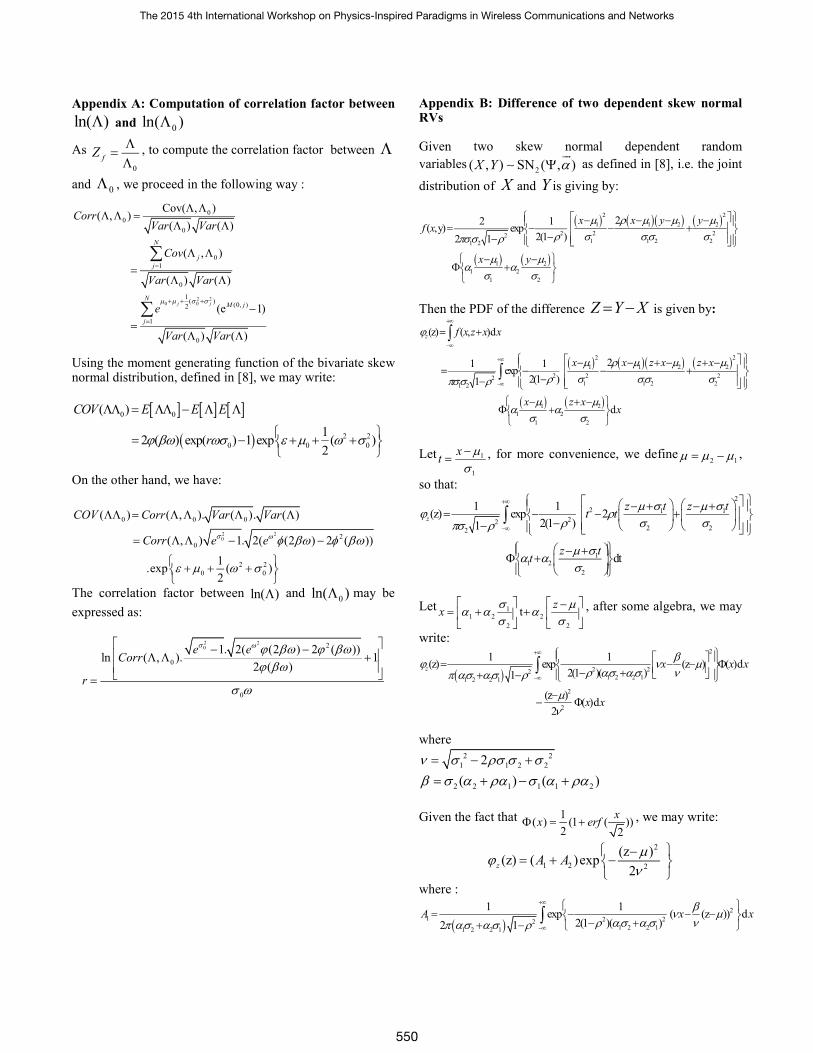
In this section, we propose to validate our formula for outage probability computation and compare it with simulation results. Fig. 2 show the outage probability for a UE located at cell edge (r=Rc) and inside the cell (r=Rc/2, r=Rc/4) with 10dB , 3.5 and 0.7 . We note that

fluctuation at the tail of SINR distribution is due to Monte

-40 -35 -30 -25 -20 -15 -10 -5 0 5 1010

-16

10-14

10-12

10-10

10-8

10-6

10-4

10-2

100

Outage Probability at r=Rc, =10dB and =3.5

SINR(dB)

Outa

ge P

robabili

ty

Simulation

Analysis

=0.7

=0.5

=0.9

=0.3

=0.1

Figure 3. Outage probability at cell edge (r=Rc) for different correlation coefficients with 10dB , 3.5

-20 -15 -10 -5 0 510

-14

10-12

10-10

10-8

10-6

10-4

10-2

100

Outage Probability at R=Rc, =3.5 and =0.4

SINR(dB)

Outa

ge P

robabili

ty

Simulation

Analysis

=4dB=3dB

=6dB

=10dB

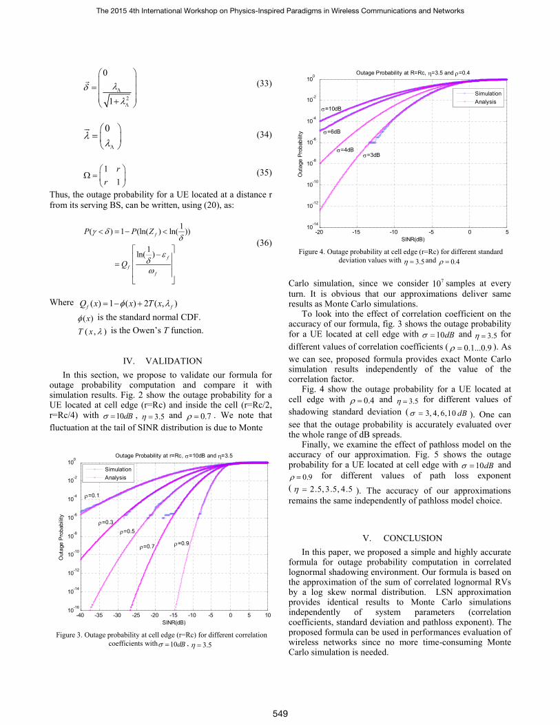
Figure 4. Outage probability at cell edge (r=Rc) for different standard deviation values with 3.5 and 0.4

Carlo simulation, since we consider 710 samples at every turn. It is obvious that our approximations deliver same results as Monte Carlo simulations.

To look into the effect of correlation coefficient on the accuracy of our formula, fig. 3 shows the outage probability for a UE located at cell edge with 10dB and 3.5 for

different values of correlation coefficients ( 0.1...0.9 ). As

we can see, proposed formula provides exact Monte Carlo simulation results independently of the value of the correlation factor.

Fig. 4 show the outage probability for a UE located at cell edge with 0.4 and 3.5 for different values of

shadowing standard deviation ( 3, 4, 6,10 dB ). One can see that the outage probability is accurately evaluated over the whole range of dB spreads.

Finally, we examine the effect of pathloss model on the accuracy of our approximation. Fig. 5 shows the outage probability for a UE located at cell edge with 10dB and

0.9 for different values of path loss exponent

( 2.5, 3.5, 4.5 ). The accuracy of our approximations remains the same independently of pathloss model choice.

V. CONCLUSION

In this paper, we proposed a simple and highly accurate formula for outage probability computation in correlated lognormal shadowing environment. Our formula is based on the approximation of the sum of correlated lognormal RVs by a log skew normal distribution. LSN approximation provides identical results to Monte Carlo simulations independently of system parameters (correlation coefficients, standard deviation and pathloss exponent). The proposed formula can be used in performances evaluation of wireless networks since no more time-consuming Monte Carlo simulation is needed.


549

Appendix A: Computation of correlation factor between

ln( ) and 0ln( )

As

0

fZ

, to compute the correlation factor between

and 0 , we proceed in the following way :

2 20 0

00

0

01

0

1( )

(0, )2

1

0

Cov( , )( , )

( ) ( )

( , )

( ) ( )

(e 1)

( ) ( )

j j

N

jj

NM j

j

CorrVar Var

Cov

Var Var

e

Var Var

Using the moment generating function of the bivariate skew normal distribution, defined in [8], we may write:

0 0

2 20 0 0

( )

12 ( ) exp( ) 1 exp ( )

2

COV E E E

r

On the other hand, we have:

2 20

0 0 0

20

2 20 0

( ) ( , ). ( ). ( )

( , ) 1. 2( (2 ) 2 ( ))

1.exp ( )

2

COV Corr Var Var

Corr e e

The correlation factor between ln( ) and 0ln( ) may be

expressed as:

2 20 2

0

0

1. 2( (2 ) 2 ( ))ln ( , ). 1

2 ( )

e eCorr

r

Appendix B: Difference of two dependent skew normal RVs Given two skew normal dependent random

variables2( , ) SN ( , )X Y

as defined in [8], i.e. the joint

distribution of X and Y is giving by:

2 2

1 1 2 2

2 2 221 1 2 21 2

1 21 2

1 2

22 1( ,y) exp

2(1 )2 1

x x y yf x

x y

Then the PDF of the difference Z Y X is given by:

2 2

1 1 2 2

2 2 221 1 2 21 2

1 21 2

1 2

(z) ( , )d

21 1exp

2(1 )1

d

z f x z x x

x x z x z x

x z xx

Let 1

1

xt

, for more convenience, we define

2 1 ,

so that: 2

2 1 122

2 22

11 2

2

1 1(z) exp 2

2(1 )1

dt

z

z t z tt t

z tt

Let 11 2 2

2 2

tz

x

, after some algebra, we may

write:

2

2 221 2 2 11 2 2 1

2

2

1 1(z) exp (z ) ( )d

2(1 )( )1

(z )( )d

2

z x x x

x x

where

2 21 1 2 22

2 2 1 1 1 2( ) ( )

Given the fact that 1( ) (1 ( ))

2 2

xx erf , we may write:

2

1 2 2

(z )(z) ( )exp

2z A A

where :

2

1 2 221 2 2 11 2 2 1

1 1exp ( (z )) d

2(1 )( )2 1A x x


550

Let (z )y x

, we may write :

2

1 2 221 2 2 11 2 2 1

2

21 2 2 1

1 1exp dy;

2(1 )( )2 1

1 1 1exp dt;

2 2 (1 )( )

1

2

A y

t t y

and

2

2 2 221 2 2 11 2 2 1

1 1exp ( (z )) ( )d

2(1 )( ) 22 1

xA x erf x

Let ( )2

xy

,

we may write :

2

2 2 221 2 2 11 2 2 1

1 1exp ( 2 (z )) (y)dy

2(1 )( )2 1A y erf

Using [11, Equation 13]:

2

2exp (ax b) (x)dx ( )

1

berf erf

a a

We may write:

2 2 2 21 2 2 1

2 2 21 2 2 1

1 (z )( )

2 2 (1 )( )

1 (z )2 ( ) 1

2 (1 )( )

A erf

So that:

2

22 2 21 2 2 1

2 (z ) (z )(z) 1 ( ) exp

2(1 )( )z

Let (z)zF denotes the cumulative distribution function of

the difference Z Y X , we have:

2

2

2

22 2 21 2 2 1

(z) ( )

2 ( )exp

2

2 ( ) ( )( )exp

2(1 )( )

z

z z

z

z

F x dx

xdx

x xdx

Let ( )xy

, we may write :

(z )

2

(z )

2

2 2 21 2 2 1

2 2 21 2 2 1

2 2 21 2 2 1

1 1(z) 2 exp y

22

2 1( ) exp y

22 (1 )( )

z z2 ( ) S ( , )

(1 )( )

z z z2 ( ) ( ) 2T( , )

(1 )( )

z

k

F dy

ydy

where ( , )T x is the Owen’s T function expressed as:

2 2

2

0

1exp (1 t )

1 2( , )

2 (1 t )

x

T x dt

We have then:

2 2 21 2 2 1

2 2 21 2 2 1

z z(z) ( ) 2T( , )

(1 )( )

zSN( , )

(1 )( )

zF

where

2 21 1 2 22

2 2 1 1 1 2( ) ( )

2 1

REFERENCES

[1] A. Safak, “Statistical analysis of the power sum of multiple correlated log-normal components”, IEEE Trans. Veh. Tech., vol. 42, pp. 58–61, Feb. 1993.

[2] S.Schwartz and Y.S. Yeh, “On the distribution function and moments of power sums with log-normal components”, Bell System Tech. J., Vol. 61, pp. 1441–1462, Sept. 1982.

[3] M. Pratesi , F. Santucci , F. Graziosi and M. Ruggieri "Outage analysis in mobile radio systems with generically correlated lognormal interferers", IEEE Trans. Commun., vol. 48, no. 3, pp.381 -385 2000.

[4] A. Safak and M. Safak "Moments of the sum of correlated log-normal random variables", Proc. IEEE 44th Vehicular Technology Conf., vol. 1, pp.140 -144 1994.

[5] M. Benhcine, R. Bouallegue, “Highly accurate log skew normal approximation to the sum of correlated lognormals ”, in the Proc. of NeTCoM 2014.


551

[6] C. L. Joshua Lam,Tho Le-Ngoc " Outage Probability with Correlated Lognormal Interferers using Log Shifted Gamma Approximation” , Wireless Personal Communications, Volume 41, Issue 2, pp 179-192, April 2007.

[7] O’Hagan A. and Leonard TBayes estimation subject to uncertainty about parameter constraints, Biometrika, 63, 201–202, 1976.

[8] Azzalini A, A class of distributions which includes the normal ones, Scand. J. Statist., 12, 171–178, 1985.

[9] M. Patefield, “Fast and accurate calculation of Owen’s t function,” J. Statist. Softw., vol. 5, no. 5, pp. 1–25, 2000.

[10] N. Balakrishnan Chin-Diew Lai, Continuous Bivariate Distributions, Springer

[11] Edward W. Ng and Murray Geller, “A Table of Integrals of the Error Functions”, Journal of Research of the National Bureau of Standards, B. Mathematical Sciences Vol. 73B, No. 1, January-March 1969

Figure 2. Outage probability at cell edge (r=Rc) and inside the cell (r=Rc/2, r=Rc/4) with 10dB , 3.5 and 0.7

Figure 5. Outage probability at cell edge (r=Rc) for different path loss exponent values with 10dB and 0.9

-10 -5 0 5 10 15 20 25 300

0.1

0.2

0.3

0.4

0.5

0.6

0.7

0.8

0.9

1Outage Probability with =9dB, =3 and =0.7

SINR(dB)

Ou

tag

e P

rob

ab

ility

Simulation

Analysis

r=Rc

r=Rc/2

r=Rc/4

-30 -20 -10 0 10 20 3010

-16

10-14

10-12

10-10

10-8

10-6

10-4

10-2

100

Outage Probability with =9dB, =3 and =0.7

SINR(dB)

Ou

tag

e P

rob

ab

ility

Simulation

Analysis

r=Rc

r=Rc/2

r=Rc/4

-8 -6 -4 -2 0 2 4 6 80

0.1

0.2

0.3

0.4

0.5

0.6

0.7

0.8

0.9

1Outage Probability at R=Rc, =10dB and =0.9

SINR(dB)

Ou

tag

e P

rob

ab

ility

Simulation

Analysis

=4.5

=3.5

=2.5

-8 -6 -4 -2 0 2 4 6 810

-7

10-6

10-5

10-4

10-3

10-2

10-1

100

Outage Probability at R=Rc, =10dB and =0.9

SINR(dB)

Ou

tag

e P

rob

ab

ility

Simulation

Analysis

=2.5

=3.5

=4.5


552

Documents

Exact evaluation of outage probability in correlated lognormal shadowing environment.dl.ifip.org/db/conf/wiopt/wiopt2015/HeineB15.pdf · 2015-10-17 · Exact Evaluation of Outage