Excel 2016: Large Data 4 Final Report

training@health.ufl.edu

Updated 3/26/2019

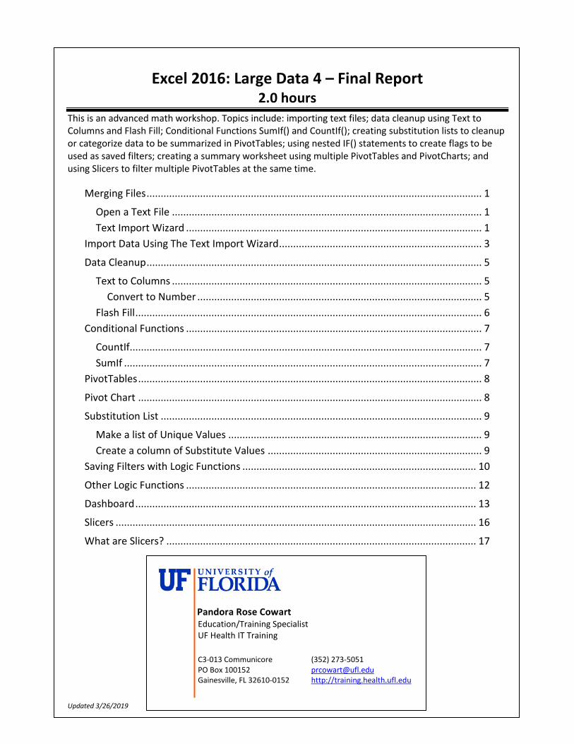
Excel 2016: Large Data 4 – Final Report 2.0 hours

This is an advanced math workshop. Topics include: importing text files; data cleanup using Text to Columns and Flash Fill; Conditional Functions SumIf() and CountIf(); creating substitution lists to cleanup or categorize data to be summarized in PivotTables; using nested IF() statements to create flags to be used as saved filters; creating a summary worksheet using multiple PivotTables and PivotCharts; and using Slicers to filter multiple PivotTables at the same time.

Merging Files ....................................................................................................................... 1

Open a Text File .............................................................................................................. 1

Text Import Wizard ......................................................................................................... 1

Import Data Using The Text Import Wizard ........................................................................ 3

Data Cleanup ....................................................................................................................... 5

Text to Columns .............................................................................................................. 5

Convert to Number ..................................................................................................... 5

Flash Fill ........................................................................................................................... 6

Conditional Functions ......................................................................................................... 7

CountIf............................................................................................................................. 7

SumIf ............................................................................................................................... 7

PivotTables .......................................................................................................................... 8

Pivot Chart .......................................................................................................................... 8

Substitution List .................................................................................................................. 9

Make a list of Unique Values .......................................................................................... 9

Create a column of Substitute Values ............................................................................ 9

Saving Filters with Logic Functions ................................................................................... 10

Other Logic Functions ....................................................................................................... 12

Dashboard ......................................................................................................................... 13

Slicers ................................................................................................................................ 16

What are Slicers? .............................................................................................................. 17

Pandora Rose Cowart

Education/Training Specialist UF Health IT Training

C3-013 Communicore (352) 273-5051 PO Box 100152 prcowart@ufl.edu Gainesville, FL 32610-0152 http://training.health.ufl.edu

1

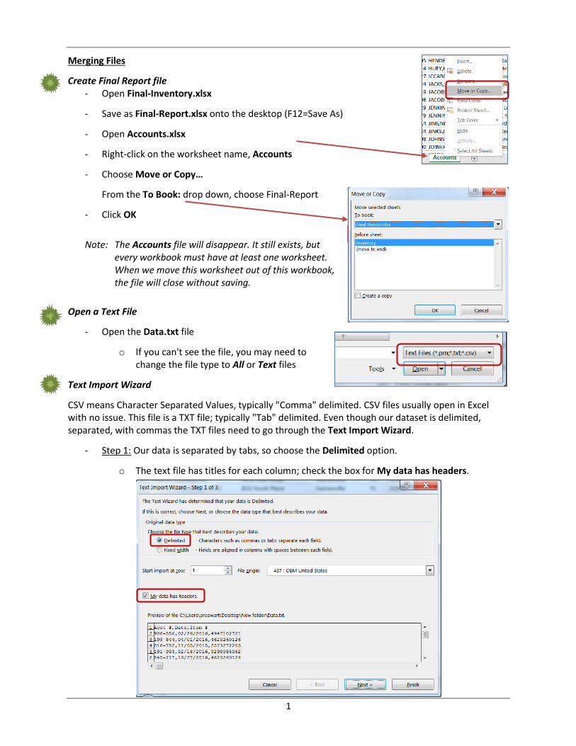
Merging Files

Create Final Report file - Open Final-Inventory.xlsx

- Save as Final-Report.xlsx onto the desktop (F12=Save As)

- Open Accounts.xlsx

- Right-click on the worksheet name, Accounts

- Choose Move or Copy…

From the To Book: drop down, choose Final-Report

- Click OK

Note: The Accounts file will disappear. It still exists, but every workbook must have at least one worksheet. When we move this worksheet out of this workbook, the file will close without saving.

Open a Text File

- Open the Data.txt file

o If you can't see the file, you may need to change the file type to All or Text files

Text Import Wizard

CSV means Character Separated Values, typically "Comma" delimited. CSV files usually open in Excel with no issue. This file is a TXT file; typically "Tab" delimited. Even though our dataset is delimited, separated, with commas the TXT files need to go through the Text Import Wizard.

- Step 1: Our data is separated by tabs, so choose the Delimited option.

o The text file has titles for each column; check the box for My data has headers.

2

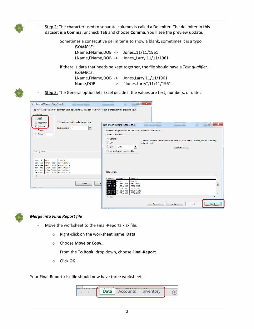
- Step 2: The character used to separate columns is called a Delimiter. The delimiter in this dataset is a Comma, uncheck Tab and choose Comma. You'll see the preview update.

Sometimes a consecutive delimiter is to show a blank, sometimes it is a typo EXAMPLE: LName,FName,DOB -> Jones,,11/11/1961 LName,FName,DOB -> Jones,,Larry,11/11/1961

If there is data that needs be kept together, the file should have a Text qualifier. EXAMPLE: LName,FName,DOB -> Jones,Larry,11/11/1961 Name,DOB -> "Jones,Larry",11/11/1961

- Step 3: The General option lets Excel decide if the values are text, numbers, or dates.

Merge into Final Report file

- Move the worksheet to the Final-Reports.xlsx file.

o Right-click on the worksheet name, Data

o Choose Move or Copy…

From the To Book: drop down, choose Final-Report

o Click OK

Your Final-Report.xlsx file should now have three worksheets.

3

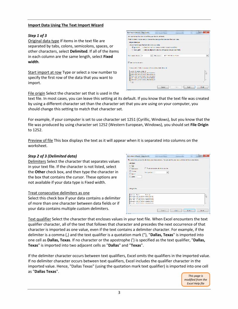
Import Data Using The Text Import Wizard Step 1 of 3 Original data type If items in the text file are separated by tabs, colons, semicolons, spaces, or other characters, select Delimited. If all of the items in each column are the same length, select Fixed width. Start import at row Type or select a row number to specify the first row of the data that you want to import. File origin Select the character set that is used in the text file. In most cases, you can leave this setting at its default. If you know that the text file was created by using a different character set than the character set that you are using on your computer, you should change this setting to match that character set. For example, if your computer is set to use character set 1251 (Cyrillic, Windows), but you know that the file was produced by using character set 1252 (Western European, Windows), you should set File Origin to 1252. Preview of file This box displays the text as it will appear when it is separated into columns on the worksheet. Step 2 of 3 (Delimited data) Delimiters Select the character that separates values in your text file. If the character is not listed, select the Other check box, and then type the character in the box that contains the cursor. These options are not available if your data type is Fixed width. Treat consecutive delimiters as one Select this check box if your data contains a delimiter of more than one character between data fields or if your data contains multiple custom delimiters. Text qualifier Select the character that encloses values in your text file. When Excel encounters the text qualifier character, all of the text that follows that character and precedes the next occurrence of that character is imported as one value, even if the text contains a delimiter character. For example, if the delimiter is a comma (,) and the text qualifier is a quotation mark ("), "Dallas, Texas" is imported into one cell as Dallas, Texas. If no character or the apostrophe (') is specified as the text qualifier, "Dallas, Texas" is imported into two adjacent cells as "Dallas" and "Texas". If the delimiter character occurs between text qualifiers, Excel omits the qualifiers in the imported value. If no delimiter character occurs between text qualifiers, Excel includes the qualifier character in the imported value. Hence, "Dallas Texas" (using the quotation mark text qualifier) is imported into one cell as "Dallas Texas". This page is

modified from the Excel Help file

4

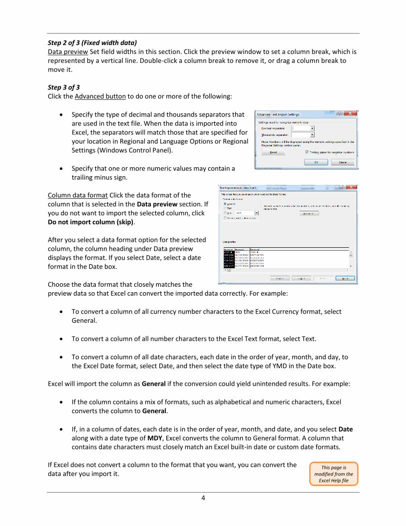
Step 2 of 3 (Fixed width data) Data preview Set field widths in this section. Click the preview window to set a column break, which is represented by a vertical line. Double-click a column break to remove it, or drag a column break to move it. Step 3 of 3 Click the Advanced button to do one or more of the following:

Specify the type of decimal and thousands separators that are used in the text file. When the data is imported into Excel, the separators will match those that are specified for your location in Regional and Language Options or Regional Settings (Windows Control Panel).

Specify that one or more numeric values may contain a trailing minus sign.

Column data format Click the data format of the column that is selected in the Data preview section. If you do not want to import the selected column, click Do not import column (skip). After you select a data format option for the selected column, the column heading under Data preview displays the format. If you select Date, select a date format in the Date box. Choose the data format that closely matches the preview data so that Excel can convert the imported data correctly. For example:

To convert a column of all currency number characters to the Excel Currency format, select General.

To convert a column of all number characters to the Excel Text format, select Text.

To convert a column of all date characters, each date in the order of year, month, and day, to the Excel Date format, select Date, and then select the date type of YMD in the Date box.

Excel will import the column as General if the conversion could yield unintended results. For example:

If the column contains a mix of formats, such as alphabetical and numeric characters, Excel converts the column to General.

If, in a column of dates, each date is in the order of year, month, and date, and you select Date along with a date type of MDY, Excel converts the column to General format. A column that contains date characters must closely match an Excel built-in date or custom date formats.

If Excel does not convert a column to the format that you want, you can convert the data after you import it.

This page is modified from the

Excel Help file

5

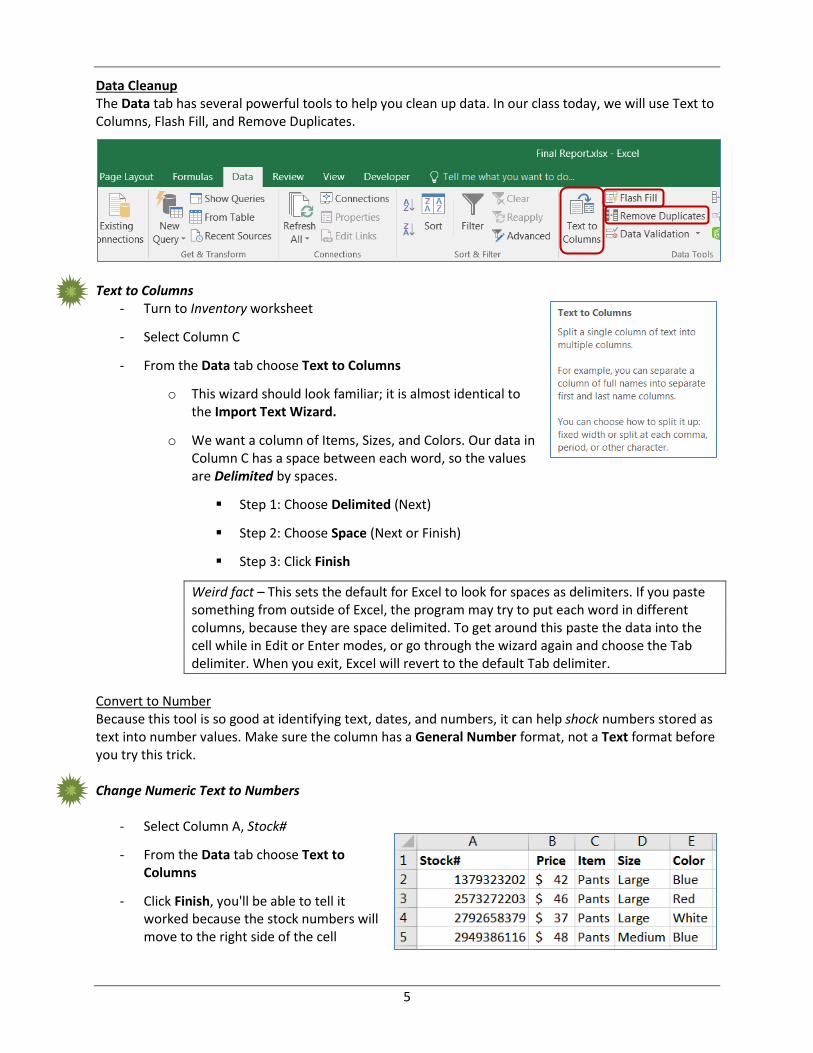
Data Cleanup The Data tab has several powerful tools to help you clean up data. In our class today, we will use Text to Columns, Flash Fill, and Remove Duplicates.

Text to Columns

- Turn to Inventory worksheet

- Select Column C

- From the Data tab choose Text to Columns

o This wizard should look familiar; it is almost identical to the Import Text Wizard.

o We want a column of Items, Sizes, and Colors. Our data in Column C has a space between each word, so the values are Delimited by spaces.

Step 1: Choose Delimited (Next)

Step 2: Choose Space (Next or Finish)

Step 3: Click Finish

Weird fact – This sets the default for Excel to look for spaces as delimiters. If you paste something from outside of Excel, the program may try to put each word in different columns, because they are space delimited. To get around this paste the data into the cell while in Edit or Enter modes, or go through the wizard again and choose the Tab delimiter. When you exit, Excel will revert to the default Tab delimiter.

Convert to Number Because this tool is so good at identifying text, dates, and numbers, it can help shock numbers stored as text into number values. Make sure the column has a General Number format, not a Text format before you try this trick. Change Numeric Text to Numbers

- Select Column A, Stock#

- From the Data tab choose Text to Columns

- Click Finish, you'll be able to tell it worked because the stock numbers will move to the right side of the cell

6

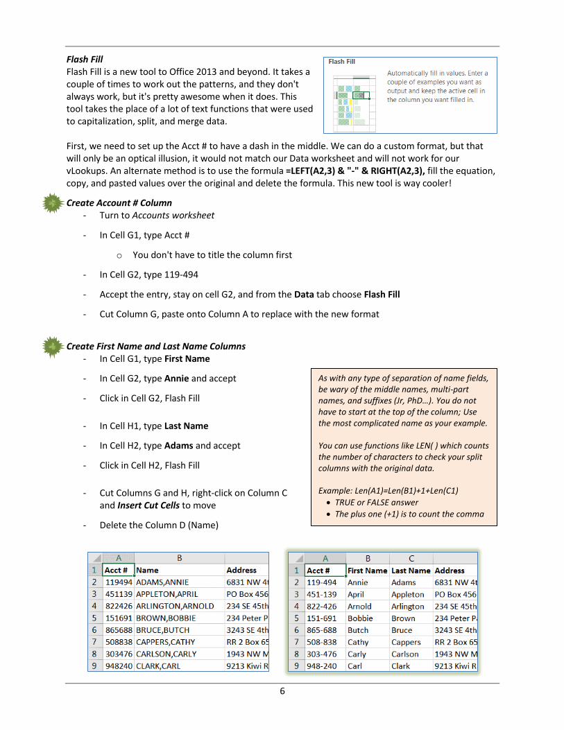
Flash Fill Flash Fill is a new tool to Office 2013 and beyond. It takes a couple of times to work out the patterns, and they don't always work, but it's pretty awesome when it does. This tool takes the place of a lot of text functions that were used to capitalization, split, and merge data. First, we need to set up the Acct # to have a dash in the middle. We can do a custom format, but that will only be an optical illusion, it would not match our Data worksheet and will not work for our vLookups. An alternate method is to use the formula =LEFT(A2,3) & "-" & RIGHT(A2,3), fill the equation, copy, and pasted values over the original and delete the formula. This new tool is way cooler!

Create Account # Column - Turn to Accounts worksheet

- In Cell G1, type Acct #

o You don't have to title the column first

- In Cell G2, type 119-494

- Accept the entry, stay on cell G2, and from the Data tab choose Flash Fill

- Cut Column G, paste onto Column A to replace with the new format

Create First Name and Last Name Columns - In Cell G1, type First Name

- In Cell G2, type Annie and accept

- Click in Cell G2, Flash Fill

- In Cell H1, type Last Name

- In Cell H2, type Adams and accept

- Click in Cell H2, Flash Fill

- Cut Columns G and H, right-click on Column C and Insert Cut Cells to move

- Delete the Column D (Name)

As with any type of separation of name fields, be wary of the middle names, multi-part names, and suffixes (Jr, PhD…). You do not have to start at the top of the column; Use the most complicated name as your example. You can use functions like LEN( ) which counts the number of characters to check your split columns with the original data. Example: Len(A1)=Len(B1)+1+Len(C1)

TRUE or FALSE answer

The plus one (+1) is to count the comma

7

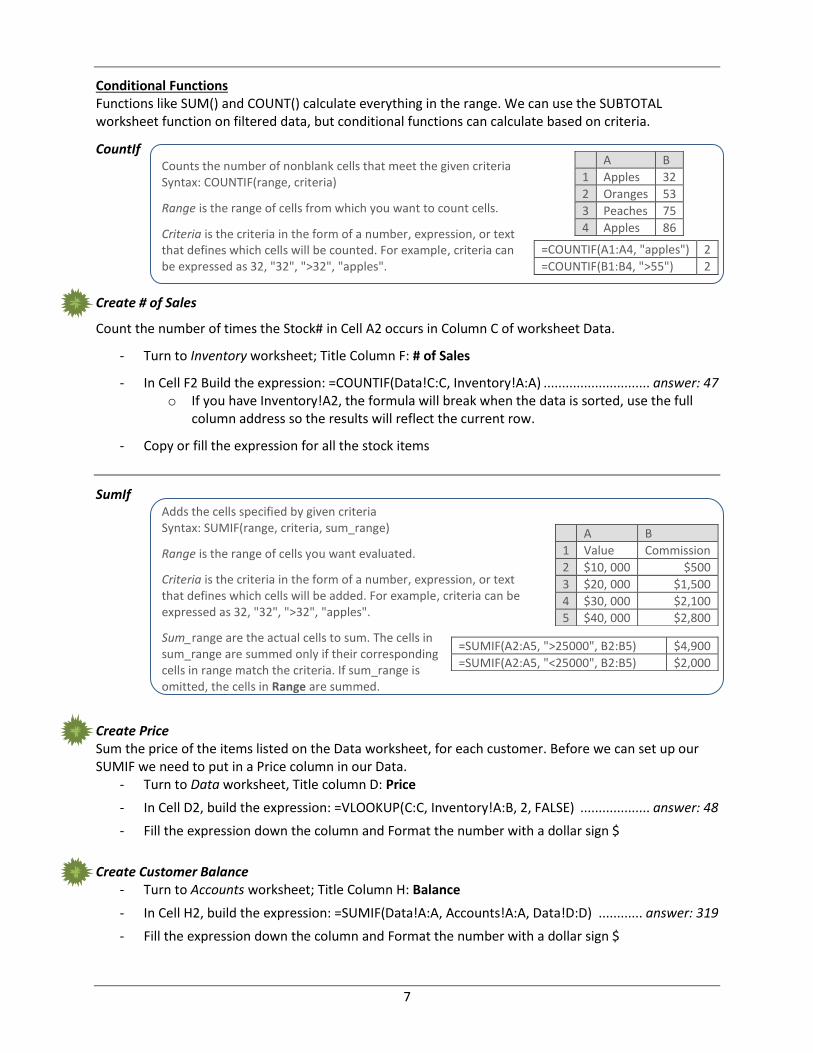
Conditional Functions Functions like SUM() and COUNT() calculate everything in the range. We can use the SUBTOTAL worksheet function on filtered data, but conditional functions can calculate based on criteria.

CountIf Counts the number of nonblank cells that meet the given criteria Syntax: COUNTIF(range, criteria)

Range is the range of cells from which you want to count cells.

Criteria is the criteria in the form of a number, expression, or text that defines which cells will be counted. For example, criteria can be expressed as 32, "32", ">32", "apples".

Create # of Sales

Count the number of times the Stock# in Cell A2 occurs in Column C of worksheet Data.

- Turn to Inventory worksheet; Title Column F: # of Sales

- In Cell F2 Build the expression: =COUNTIF(Data!C:C, Inventory!A:A) ............................. answer: 47 o If you have Inventory!A2, the formula will break when the data is sorted, use the full

column address so the results will reflect the current row.

- Copy or fill the expression for all the stock items

SumIf Adds the cells specified by given criteria Syntax: SUMIF(range, criteria, sum_range)

Range is the range of cells you want evaluated.

Criteria is the criteria in the form of a number, expression, or text that defines which cells will be added. For example, criteria can be expressed as 32, "32", ">32", "apples".

Sum_range are the actual cells to sum. The cells in sum_range are summed only if their corresponding cells in range match the criteria. If sum_range is omitted, the cells in Range are summed.

Create Price Sum the price of the items listed on the Data worksheet, for each customer. Before we can set up our SUMIF we need to put in a Price column in our Data.

- Turn to Data worksheet, Title column D: Price

- In Cell D2, build the expression: =VLOOKUP(C:C, Inventory!A:B, 2, FALSE) ................... answer: 48

- Fill the expression down the column and Format the number with a dollar sign $

Create Customer Balance

- Turn to Accounts worksheet; Title Column H: Balance

- In Cell H2, build the expression: =SUMIF(Data!A:A, Accounts!A:A, Data!D:D) ............ answer: 319

- Fill the expression down the column and Format the number with a dollar sign $

A B

1 Apples 32

2 Oranges 53

3 Peaches 75

4 Apples 86

=COUNTIF(A1:A4, "apples") 2

=COUNTIF(B1:B4, ">55") 2

A B

1 Value Commission

2 $10, 000 $500

3 $20, 000 $1,500

4 $30, 000 $2,100

5 $40, 000 $2,800

=SUMIF(A2:A5, ">25000", B2:B5) $4,900

=SUMIF(A2:A5, "<25000", B2:B5) $2,000

8

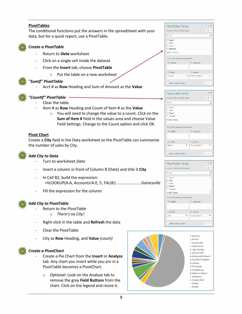
PivotTables The conditional functions put the answers in the spreadsheet with your data, but for a quick report, use a PivotTable. Create a PivotTable

- Return to Data worksheet

- Click on a single cell inside the dataset

- From the Insert tab, choose PivotTable

o Put the table on a new worksheet

"SumIf" PivotTable - Acct # as Row Heading and Sum of Amount as the Value

"CountIf" PivotTable

- Clear the table - Item # as Row Heading and Count of Item # as the Value

o You will need to change the value to a count. Click on the Sum of Item # field in the values area and choose Value Field Settings. Change to the Count option and click OK.

Pivot Chart Create a City field in the Data worksheet so the PivotTable can summarize the number of sales by City. Add City to Data

- Turn to worksheet Data

- Insert a column in front of Column B (Date) and title it City

- In Cell B2, build the expression: =VLOOKUP(A:A, Accounts!A:E, 5, FALSE) ....................... Gainesville

- Fill the expression for the column

Add City to PivotTable - Return to the PivotTable

o There's no City!

- Right-click in the table and Refresh the data

- Clear the PivotTable

- City as Row Heading, and Value (count)

Create a PivotChart - Create a Pie Chart from the Insert or Analyze

tab. Any chart you insert while you are in a PivotTable becomes a PivotChart.

o Optional: Look on the Analyze tab to remove the grey Field Buttons from the chart. Click on the legend and resize it.

9

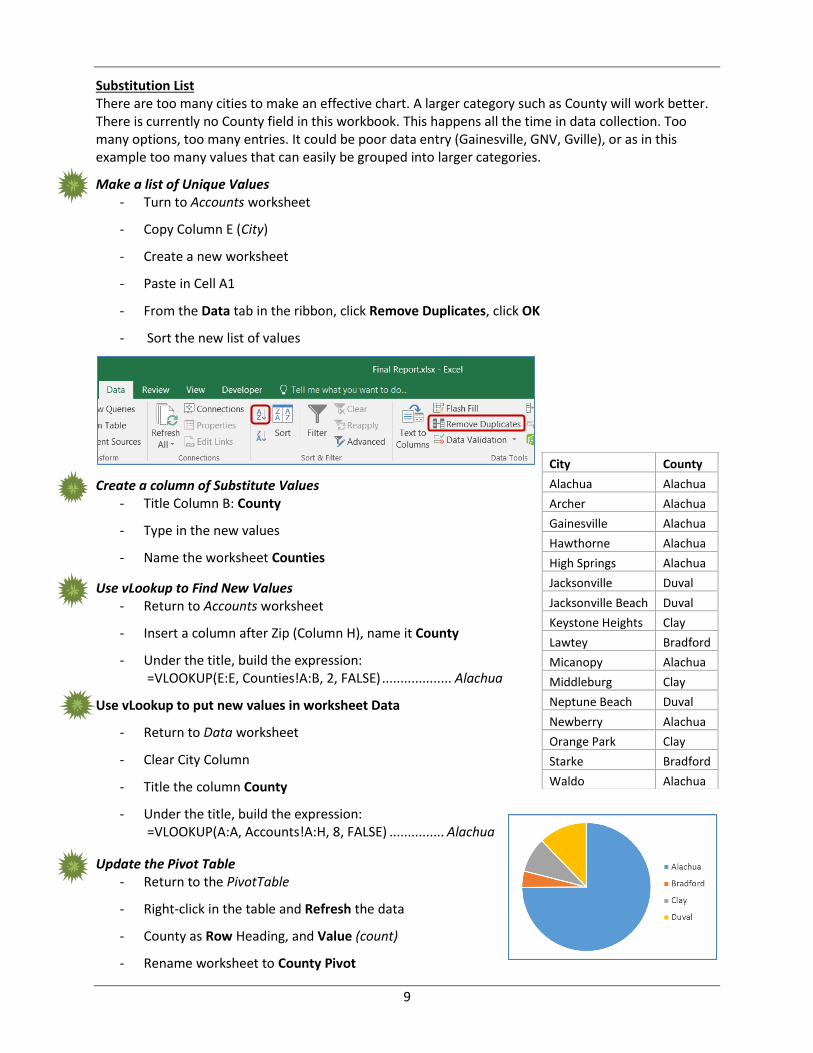
Substitution List There are too many cities to make an effective chart. A larger category such as County will work better. There is currently no County field in this workbook. This happens all the time in data collection. Too many options, too many entries. It could be poor data entry (Gainesville, GNV, Gville), or as in this example too many values that can easily be grouped into larger categories.

Make a list of Unique Values - Turn to Accounts worksheet

- Copy Column E (City)

- Create a new worksheet

- Paste in Cell A1

- From the Data tab in the ribbon, click Remove Duplicates, click OK

- Sort the new list of values

Create a column of Substitute Values - Title Column B: County

- Type in the new values

- Name the worksheet Counties

Use vLookup to Find New Values - Return to Accounts worksheet

- Insert a column after Zip (Column H), name it County

- Under the title, build the expression: =VLOOKUP(E:E, Counties!A:B, 2, FALSE) ................... Alachua

Use vLookup to put new values in worksheet Data

- Return to Data worksheet

- Clear City Column

- Title the column County

- Under the title, build the expression: =VLOOKUP(A:A, Accounts!A:H, 8, FALSE) ............... Alachua

Update the Pivot Table - Return to the PivotTable

- Right-click in the table and Refresh the data

- County as Row Heading, and Value (count)

- Rename worksheet to County Pivot

City County

Alachua Alachua

Archer Alachua

Gainesville Alachua

Hawthorne Alachua

High Springs Alachua

Jacksonville Duval

Jacksonville Beach Duval

Keystone Heights Clay

Lawtey Bradford

Micanopy Alachua

Middleburg Clay

Neptune Beach Duval

Newberry Alachua

Orange Park Clay

Starke Bradford

Waldo Alachua

10

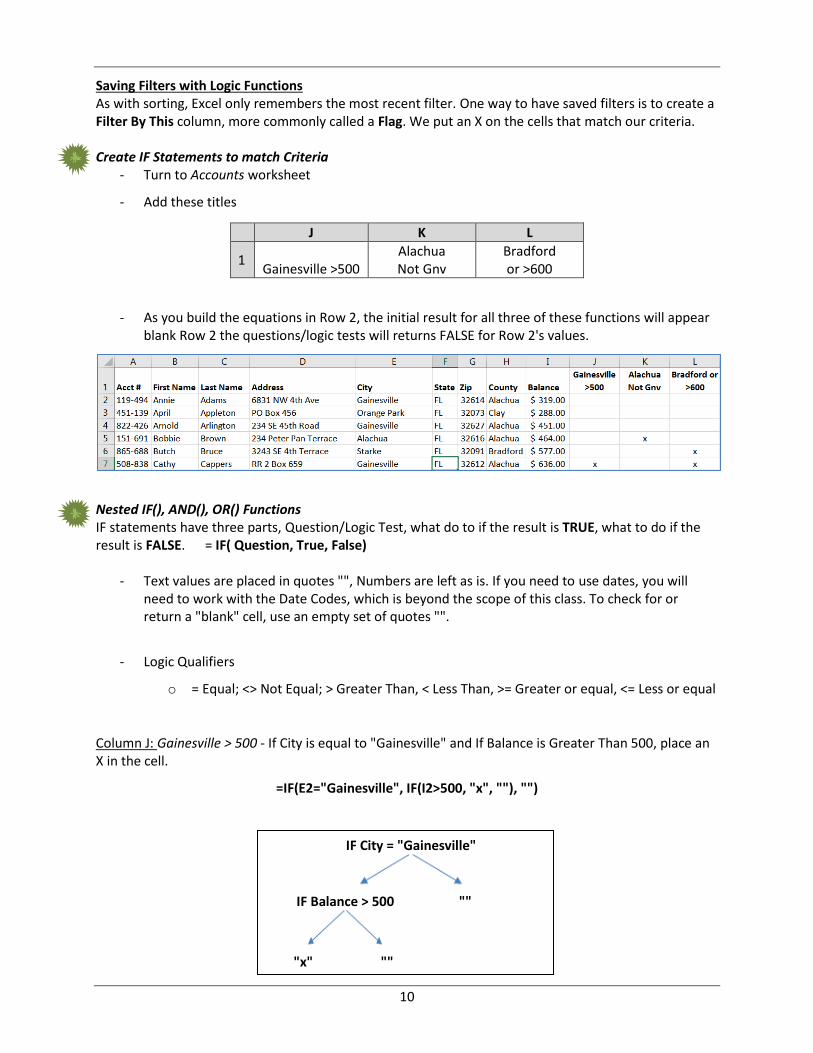
Saving Filters with Logic Functions As with sorting, Excel only remembers the most recent filter. One way to have saved filters is to create a Filter By This column, more commonly called a Flag. We put an X on the cells that match our criteria. Create IF Statements to match Criteria

- Turn to Accounts worksheet

- Add these titles

J K L

1 Gainesville >500

Alachua Not Gnv

Bradford or >600

- As you build the equations in Row 2, the initial result for all three of these functions will appear blank Row 2 the questions/logic tests will returns FALSE for Row 2's values.

Nested IF(), AND(), OR() Functions IF statements have three parts, Question/Logic Test, what do to if the result is TRUE, what to do if the result is FALSE. = IF( Question, True, False)

- Text values are placed in quotes "", Numbers are left as is. If you need to use dates, you will need to work with the Date Codes, which is beyond the scope of this class. To check for or return a "blank" cell, use an empty set of quotes "".

- Logic Qualifiers

o = Equal; <> Not Equal; > Greater Than, < Less Than, >= Greater or equal, <= Less or equal

Column J: Gainesville > 500 - If City is equal to "Gainesville" and If Balance is Greater Than 500, place an X in the cell.

=IF(E2="Gainesville", IF(I2>500, "x", ""), "")

IF City = "Gainesville"

IF Balance > 500 ""

"x" ""

11

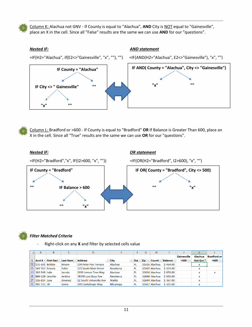
Column K: Alachua not GNV - If County is equal to "Alachua", AND City is NOT equal to "Gainesville", place an X in the cell. Since all "False" results are the same we can use AND for our "questions".

Nested IF: AND statement

=IF(H2="Alachua", if(E2<>"Gainesville", "x", ""), "") =IF(AND(H2="Alachua", E2<>"Gainesville"), "x", "")

Column L: Bradford or >600 - If County is equal to "Bradford" OR If Balance is Greater Than 600, place an X in the cell. Since all "True" results are the same we can use OR for our "questions".

Nested IF: OR statement

=IF(H2="Bradford","x", IF(I2>600, "x", "")) =IF(OR(H2="Bradford", I2>600), "x", "")

Filter Matched Criteria

- Right-click on any X and filter by selected cells value

IF AND( County = "Alachua", City <> "Gainesville")

"x" ""

IF County = "Alachua"

IF City <> " Gainesville" ""

"x" ""

IF OR( County = "Bradford", City <> 500)

"" "x"

IF County = "Bradford"

"" IF Balance > 600

"" "x"

12

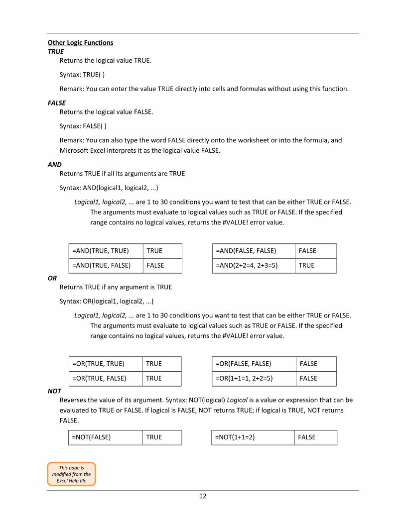
Other Logic Functions TRUE

Returns the logical value TRUE.

Syntax: TRUE( )

Remark: You can enter the value TRUE directly into cells and formulas without using this function.

FALSE Returns the logical value FALSE.

Syntax: FALSE( )

Remark: You can also type the word FALSE directly onto the worksheet or into the formula, and

Microsoft Excel interprets it as the logical value FALSE.

AND Returns TRUE if all its arguments are TRUE

Syntax: AND(logical1, logical2, ...)

Logical1, logical2, ... are 1 to 30 conditions you want to test that can be either TRUE or FALSE.

The arguments must evaluate to logical values such as TRUE or FALSE. If the specified

range contains no logical values, returns the #VALUE! error value.

=AND(TRUE, TRUE) TRUE =AND(FALSE, FALSE) FALSE

=AND(TRUE, FALSE) FALSE =AND(2+2=4, 2+3=5) TRUE

OR Returns TRUE if any argument is TRUE

Syntax: OR(logical1, logical2, ...)

Logical1, logical2, ... are 1 to 30 conditions you want to test that can be either TRUE or FALSE.

The arguments must evaluate to logical values such as TRUE or FALSE. If the specified

range contains no logical values, returns the #VALUE! error value.

=OR(TRUE, TRUE) TRUE =OR(FALSE, FALSE) FALSE

=OR(TRUE, FALSE) TRUE =OR(1+1=1, 2+2=5) FALSE

NOT Reverses the value of its argument. Syntax: NOT(logical) Logical is a value or expression that can be

evaluated to TRUE or FALSE. If logical is FALSE, NOT returns TRUE; if logical is TRUE, NOT returns

FALSE.

=NOT(FALSE) TRUE =NOT(1+1=2) FALSE

This page is modified from the

Excel Help file

13

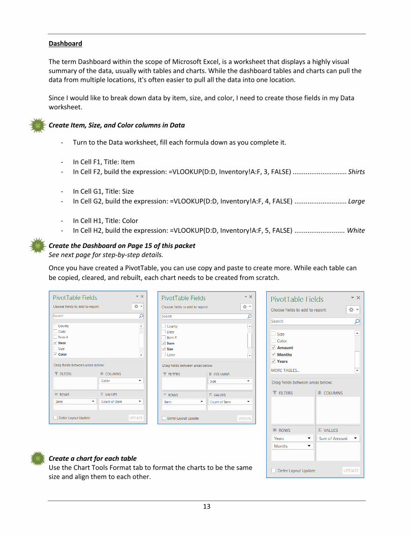
Dashboard The term Dashboard within the scope of Microsoft Excel, is a worksheet that displays a highly visual summary of the data, usually with tables and charts. While the dashboard tables and charts can pull the data from multiple locations, it's often easier to pull all the data into one location. Since I would like to break down data by item, size, and color, I need to create those fields in my Data worksheet. Create Item, Size, and Color columns in Data

- Turn to the Data worksheet, fill each formula down as you complete it.

- In Cell F1, Title: Item

- In Cell F2, build the expression: =VLOOKUP(D:D, Inventory!A:F, 3, FALSE) ............................. Shirts

- In Cell G1, Title: Size

- In Cell G2, build the expression: =VLOOKUP(D:D, Inventory!A:F, 4, FALSE) ............................ Large

- In Cell H1, Title: Color

- In Cell H2, build the expression: =VLOOKUP(D:D, Inventory!A:F, 5, FALSE) ........................... White

Create the Dashboard on Page 15 of this packet See next page for step-by-step details.

Once you have created a PivotTable, you can use copy and paste to create more. While each table can

be copied, cleared, and rebuilt, each chart needs to be created from scratch.

Create a chart for each table Use the Chart Tools Format tab to format the charts to be the same size and align them to each other.

14

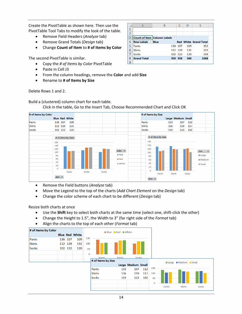
Create the PivotTable as shown here. Then use the PivotTable Tool Tabs to modify the look of the table.

Remove Field Headers (Analyze tab)

Remove Grand Totals (Design tab)

Change Count of Item to # of Items by Color The second PivotTable is similar.

Copy the # of Items by Color PivotTable

Paste in Cell J3

From the column headings, remove the Color and add Size

Rename to # of Items by Size Delete Rows 1 and 2. Build a (clustered) column chart for each table.

Click in the table, Go to the Insert Tab, Choose Recommended Chart and Click OK

Remove the Field buttons (Analyze tab)

Move the Legend to the top of the charts (Add Chart Element on the Design tab)

Change the color scheme of each chart to be different (Design tab) Resize both charts at once

Use the Shift key to select both charts at the same time (select one, shift-click the other)

Change the Height to 1.5", the Width to 3" (far right side of the Format tab)

Align the charts to the top of each other (Format tab)

15

SAVE YOUR FILE!

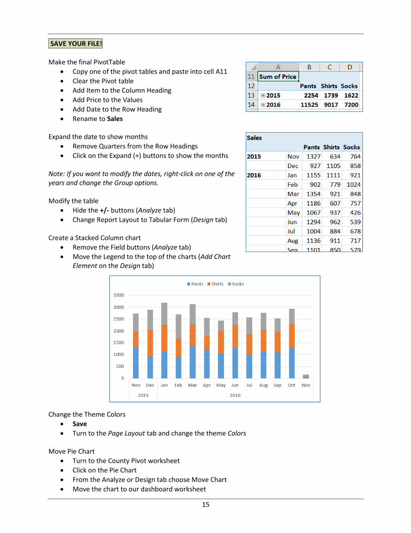
Make the final PivotTable

Copy one of the pivot tables and paste into cell A11

Clear the Pivot table

Add Item to the Column Heading

Add Price to the Values

Add Date to the Row Heading

Rename to Sales Expand the date to show months

Remove Quarters from the Row Headings

Click on the Expand (+) buttons to show the months Note: If you want to modify the dates, right-click on one of the years and change the Group options. Modify the table

Hide the +/- buttons (Analyze tab)

Change Report Layout to Tabular Form (Design tab) Create a Stacked Column chart

Remove the Field buttons (Analyze tab)

Move the Legend to the top of the charts (Add Chart Element on the Design tab)

Change the Theme Colors

Save

Turn to the Page Layout tab and change the theme Colors Move Pie Chart

Turn to the County Pivot worksheet

Click on the Pie Chart

From the Analyze or Design tab choose Move Chart

Move the chart to our dashboard worksheet

16

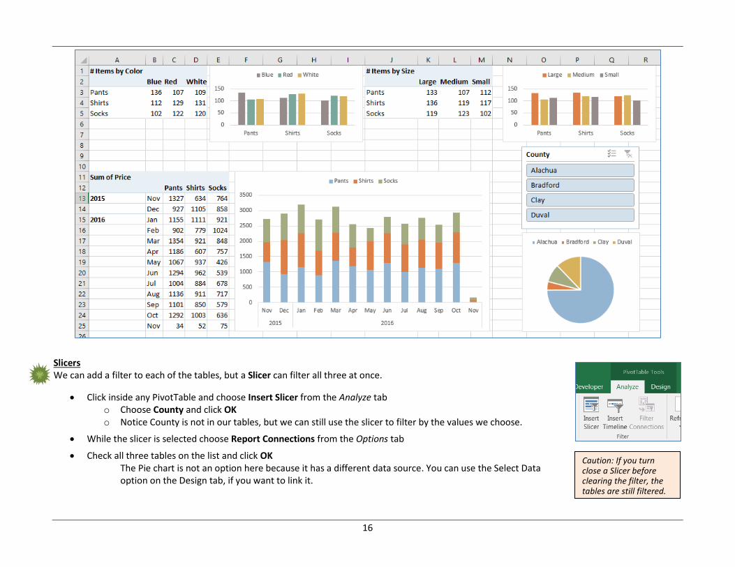
Slicers We can add a filter to each of the tables, but a Slicer can filter all three at once.

Click inside any PivotTable and choose Insert Slicer from the Analyze tab o Choose County and click OK o Notice County is not in our tables, but we can still use the slicer to filter by the values we choose.

While the slicer is selected choose Report Connections from the Options tab

Check all three tables on the list and click OK o The Pie chart is not an option here because it has a different data source. You can use the Select Data

option on the Design tab, if you want to link it.

Caution: If you turn close a Slicer before clearing the filter, the tables are still filtered.

17

What are Slicers? Slicers are easy-to-use filtering components that contain a set of buttons that enable you to quickly filter

the data in a PivotTable report, without the need to open drop-down lists to find the items that you

want to filter.

When you use a regular PivotTable report filter to filter on multiple items, the filter indicates only that

multiple items are filtered, and you have to open a drop-down list to find the filtering details. However,

a slicer clearly labels the filter that is applied and provides details so that you can easily understand the

data that is displayed in the filtered PivotTable report.

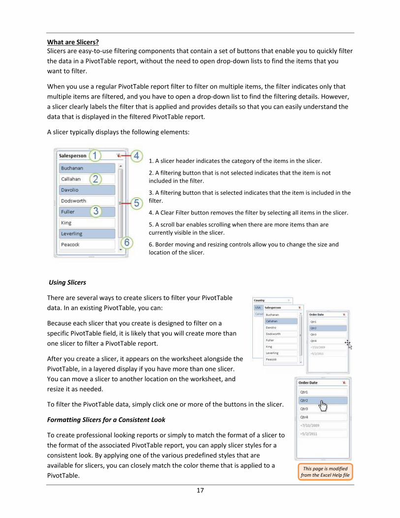
A slicer typically displays the following elements:

1. A slicer header indicates the category of the items in the slicer.

2. A filtering button that is not selected indicates that the item is not included in the filter.

3. A filtering button that is selected indicates that the item is included in the filter.

4. A Clear Filter button removes the filter by selecting all items in the slicer.

5. A scroll bar enables scrolling when there are more items than are currently visible in the slicer.

6. Border moving and resizing controls allow you to change the size and location of the slicer.

Using Slicers

There are several ways to create slicers to filter your PivotTable

data. In an existing PivotTable, you can:

Because each slicer that you create is designed to filter on a

specific PivotTable field, it is likely that you will create more than

one slicer to filter a PivotTable report.

After you create a slicer, it appears on the worksheet alongside the

PivotTable, in a layered display if you have more than one slicer.

You can move a slicer to another location on the worksheet, and

resize it as needed.

To filter the PivotTable data, simply click one or more of the buttons in the slicer.

Formatting Slicers for a Consistent Look

To create professional looking reports or simply to match the format of a slicer to

the format of the associated PivotTable report, you can apply slicer styles for a

consistent look. By applying one of the various predefined styles that are

available for slicers, you can closely match the color theme that is applied to a

PivotTable. This page is modified

from the Excel Help file

18

Sharing slicers between PivotTables

When you have many different PivotTables in one report, such as a Business Intelligence (BI) report that

you are working with, it is likely that you will want to apply the same filter to some or all of those

PivotTables. You can share a slicer that you created in one PivotTable with other PivotTables. No need to

duplicate the filter for each PivotTable!

When you share a slicer, you are creating a connection to another PivotTable that contains the slicer that

you want to use. Any changes that you make to a shared slicer are immediately reflected in all PivotTables

that are connected to that slicer. For example, if you use a Country slicer in PivotTable1 to filter data for a

specific country, PivotTable2 that also uses that slicer will display data for the same country.

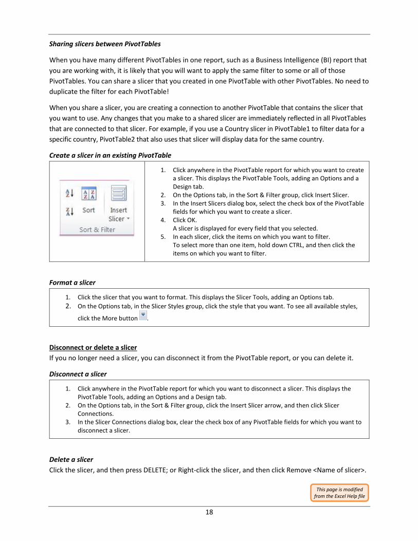
Create a slicer in an existing PivotTable

1. Click anywhere in the PivotTable report for which you want to create a slicer. This displays the PivotTable Tools, adding an Options and a Design tab.

2. On the Options tab, in the Sort & Filter group, click Insert Slicer. 3. In the Insert Slicers dialog box, select the check box of the PivotTable

fields for which you want to create a slicer. 4. Click OK.

A slicer is displayed for every field that you selected. 5. In each slicer, click the items on which you want to filter.

To select more than one item, hold down CTRL, and then click the items on which you want to filter.

Format a slicer

1. Click the slicer that you want to format. This displays the Slicer Tools, adding an Options tab.

2. On the Options tab, in the Slicer Styles group, click the style that you want. To see all available styles,

click the More button .

Disconnect or delete a slicer

If you no longer need a slicer, you can disconnect it from the PivotTable report, or you can delete it.

Disconnect a slicer

1. Click anywhere in the PivotTable report for which you want to disconnect a slicer. This displays the PivotTable Tools, adding an Options and a Design tab.

2. On the Options tab, in the Sort & Filter group, click the Insert Slicer arrow, and then click Slicer Connections.

3. In the Slicer Connections dialog box, clear the check box of any PivotTable fields for which you want to disconnect a slicer.

Delete a slicer

Click the slicer, and then press DELETE; or Right-click the slicer, and then click Remove <Name of slicer>.

This page is modified from the Excel Help file