Embed Size (px)
Citation preview
GE 2112 Fundamentals of Computing and Programming
Creating an Excel XP Spreadsheet using Windows 98/2000/Me/XP
Starting Excel XP
In the following exercises you will learn some of the necessary steps to create a spreadsheet
using Microsoft Excel XP for Windows 98, 2000, Me, and XP. You will learn not only how to type various items into the spreadsheet, but also how to copy columns, widen columns, fill columns, add, subtract, multiply, divide, do graphics and a variety of other “things.”
To begin, load the spreadsheet by quickly clicking twice on the Excel XP
Windows Icon in the Windows Screen. If you do not see an Excel Icon,
click-on the Start Button in the lower left corner of the screen, move the
cursor up to Programs, and then move to Microsoft Excel and click-on it.
A spreadsheet is a “number manipulator.” To make the manipulation of numbers easier all
spreadsheets are organized into rows and columns. Your initial spreadsheet will look something like the one below:
Notice that the “main” part of the spreadsheet is composed of Rows (Labeled 1, 2, 3, 4, etc.)
and Columns (Labeled A, B, C, D, etc.). There are a lot of rows and columns in a spreadsheet.
The “intersection” of each row and column is called a cell. In the image above the cursor is on
the “home” cell – A1. Notice Row 1 and Column A are “bold.” This indicates what is called
the “address of the cell. Notice right above cell A1, that A1 is displayed in a small box called
the Name Box. Whenever you “click” on a cell the address of that cell will be shown in the Name Box.
GE 2112 Fundamentals of Computing and Programming
In this tutorial, whenever we indicate that you need to click the mouse, it will mean to click the left mouse button – unless we indicate that you should click the right mouse button. So, always “click left” unless we tell you otherwise.
Moving Around the Spreadsheet
You can move around the spreadsheet/cells by clicking your mouse on various cells, or by using
the up, down, right and left arrow movement keys on the keyboard. Or, you can move up
and down by using the “elevator” bars on the right and bottom of the spreadsheet. Go ahead
and move around the spreadsheet. Hold down the down arrow key on the keyboard for a
few seconds – then click-on a cell. Notice how the Name Box always tells you “where you
are.” Now hold down the right arrow key on the keyboard for a few seconds. Notice how the
alphabet changes from single letters (A, B, C,. …. Z) to several letter combinations (AA,
AB, AC). There are hundreds of columns and thousands of rows in a spreadsheet. Anytime
you desire to return to the Home Cell (A1) simply click-in the Name Box and type-in A1.
Then tap the Enter key and you will go to cell A1. You can go to any cell by this method. Simply type-in a row and column, tap the Enter key, and you’ll go to that cell.
Now that you have the “feel” of how to move around Excel spreadsheet, go to the cells as
indicated below and type-in the following:
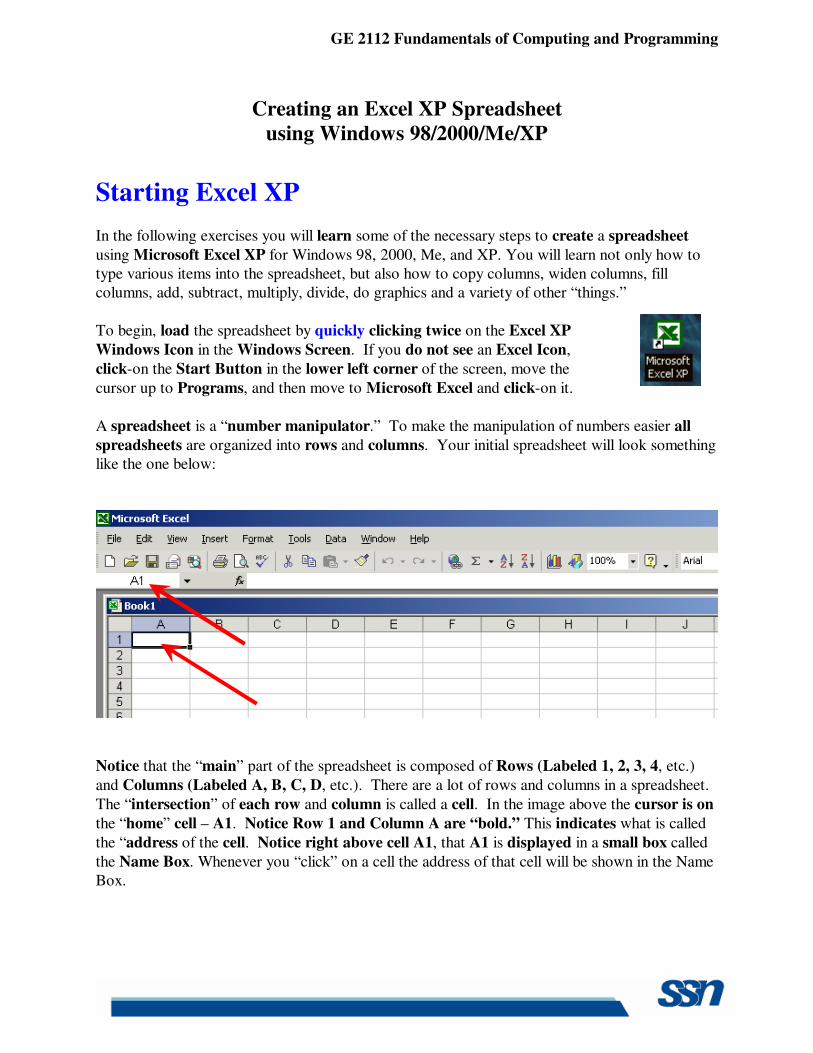
Cl (Your Name)'s Budget. It should look similar to the image below. Do not tap Enter when you finish
Look at cells C1 and D1. Notice how your entry has spilled over from C1 into D1.
Sometimes this is a problem, and sometimes it is not. Tap the Enter key and then click-on cell
D1 and type-in the word BONZO and tap Enter key.
GE 2112 Fundamentals of Computing and Programming
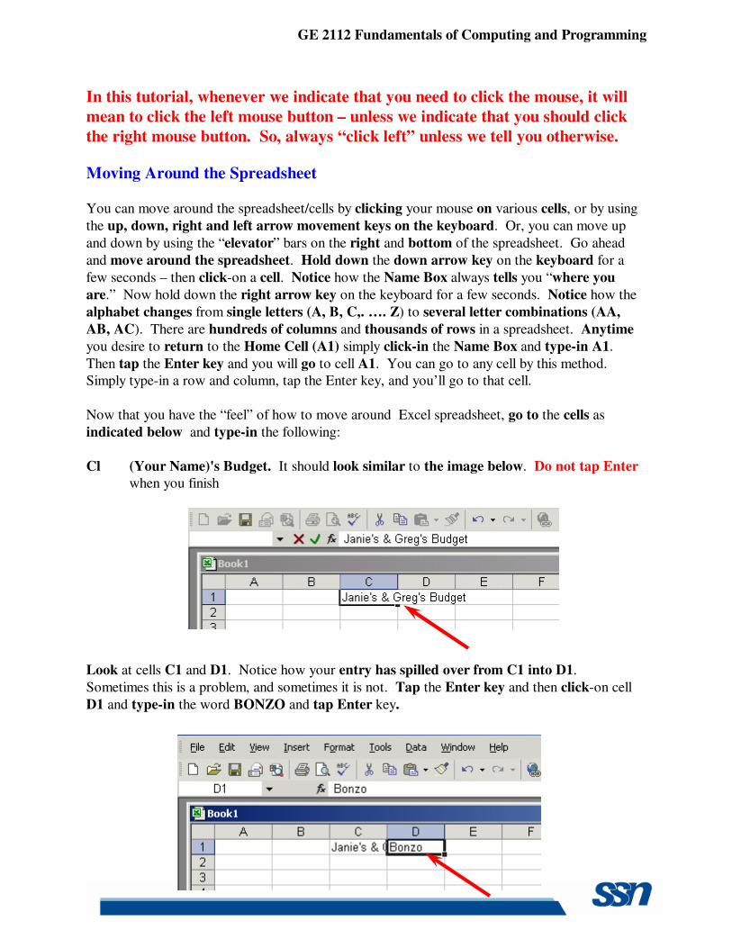
Notice how Bonzo now COVERS the right part of your original entry!! Now move back to
cell C1 and click-on it. Look at the upper part of the spreadsheet, just above the cells where you
typed Bonzo. Your name and the word budget are still there! Bonzo only COVERED the
portion in cell D1. See the image and arrow below.
There are several ways to take care of this. For the moment move back to cell D1 and click-on
cell D1. Tap the Delete key (above the arrow movement keys on the keyboard). Notice that
Bonzo disappears and your entire entry reappears. This is one way to expose the entry. We'll look at some others as we go along.
Now we'll continue making some entries. Move to the following cells and type-in the
information indicated.
If you happen to make a mistake simply retype the entries. Later on we'll see how to edit mistakes. Any time you want to replace something in a cell you can simply retype a new entry and it will replace the old one.
Cell Type-in
A3 INCOME
B4 Parents B5 Job B6 Investments B7 Total A10 EXPENSES B11 Food B12 Beverages B13 Parties B14 Miscellaneous B15 Total
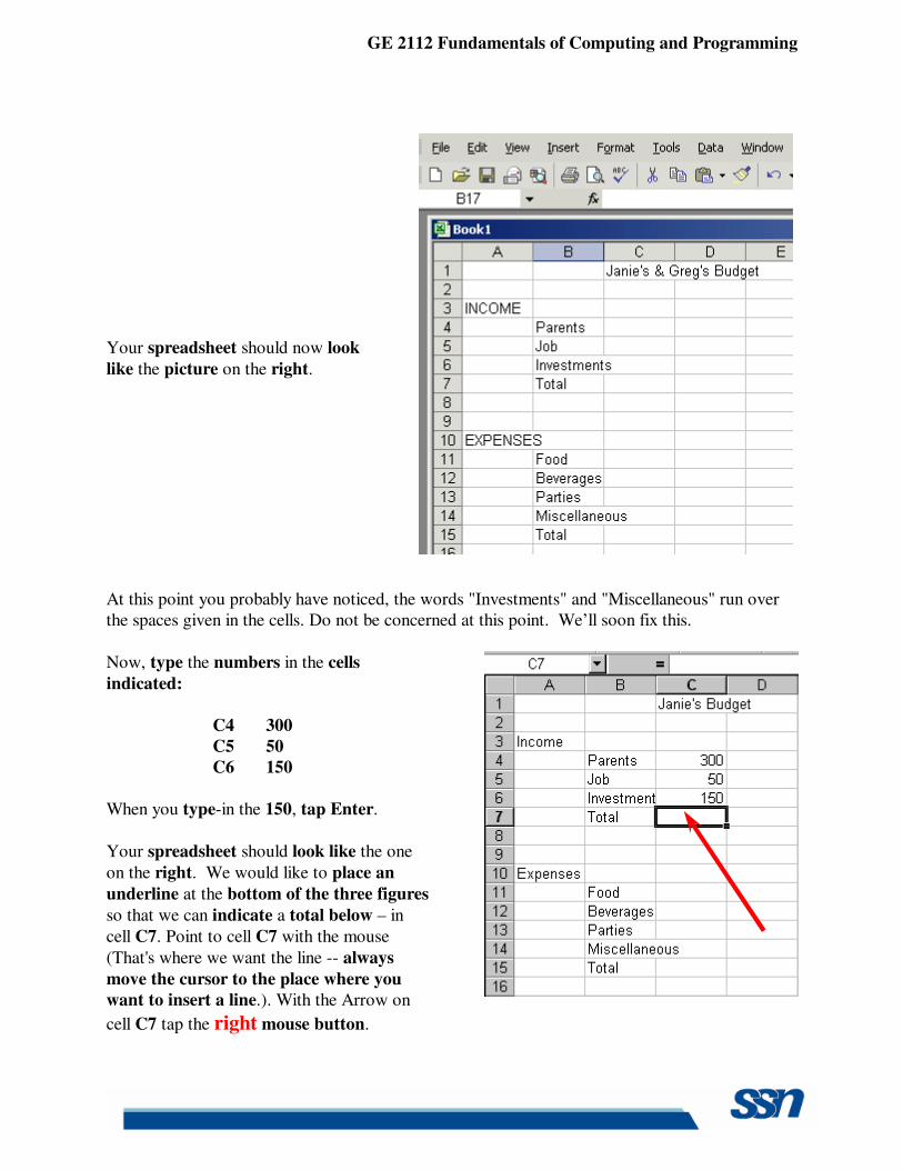
GE 2112 Fundamentals of Computing and Programming
Your spreadsheet should now look
like the picture on the right.
At this point you probably have noticed, the words "Investments" and "Miscellaneous" run over the spaces given in the cells. Do not be concerned at this point. We’ll soon fix this.
Now, type the numbers in the cells
indicated: C4 300 C5 50 C6 150
When you type-in the 150, tap Enter.
Your spreadsheet should look like the one
on the right. We would like to place an
underline at the bottom of the three figures
so that we can indicate a total below – in
cell C7. Point to cell C7 with the mouse
(That's where we want the line -- always
move the cursor to the place where you want to insert a line.). With the Arrow on
cell C7 tap the right mouse button.
GE 2112 Fundamentals of Computing and Programming
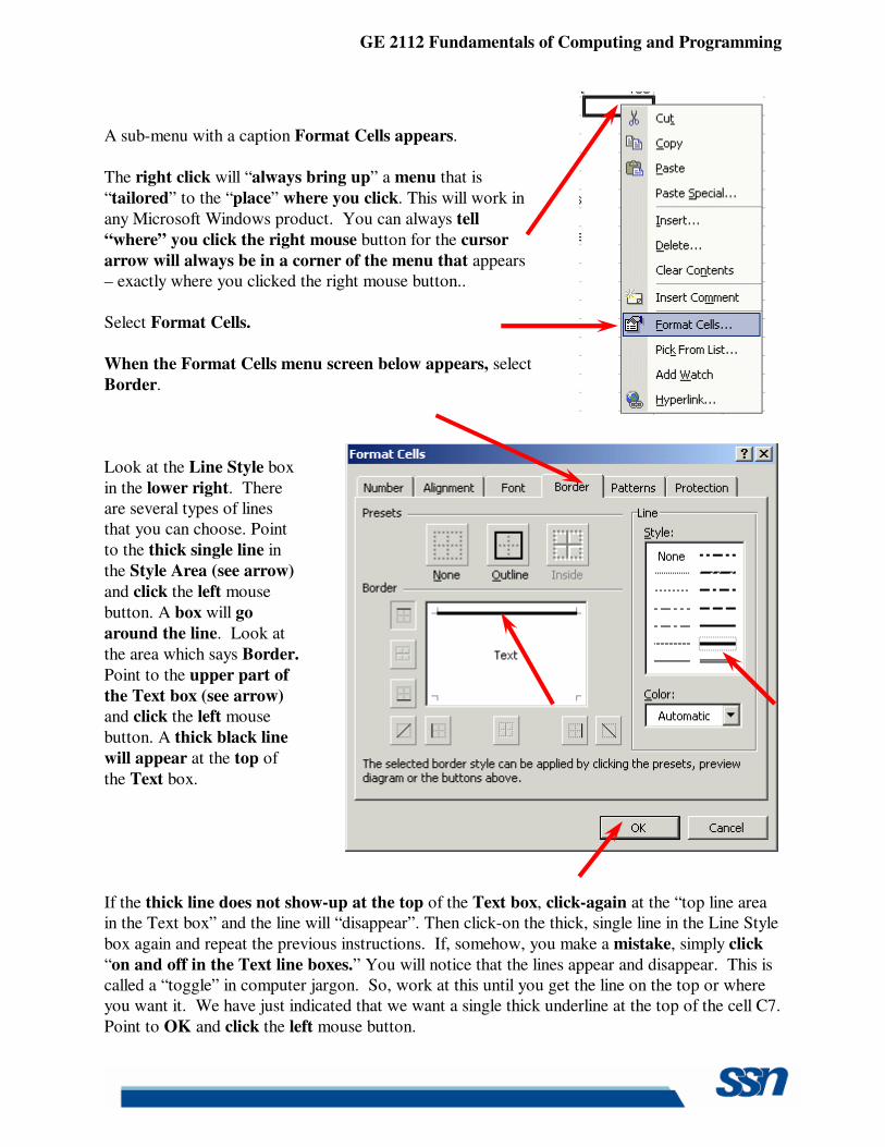
A sub-menu with a caption Format Cells appears.
The right click will “always bring up” a menu that is
“tailored” to the “place” where you click. This will work in
any Microsoft Windows product. You can always tell
“where” you click the right mouse button for the cursor
arrow will always be in a corner of the menu that appears – exactly where you clicked the right mouse button..
Select Format Cells.
When the Format Cells menu screen below appears, select
Border.
Look at the Line Style box
in the lower right. There are several types of lines that you can choose. Point
to the thick single line in
the Style Area (see arrow)
and click the left mouse
button. A box will go
around the line. Look at
the area which says Border.
Point to the upper part of
the Text box (see arrow) and click the left mouse
button. A thick black line
will appear at the top of
the Text box.
If the thick line does not show-up at the top of the Text box, click-again at the “top line area in the Text box” and the line will “disappear”. Then click-on the thick, single line in the Line Style
box again and repeat the previous instructions. If, somehow, you make a mistake, simply click
“on and off in the Text line boxes.” You will notice that the lines appear and disappear. This is called a “toggle” in computer jargon. So, work at this until you get the line on the top or where you want it. We have just indicated that we want a single thick underline at the top of the cell C7.
Point to OK and click the left mouse button.
GE 2112 Fundamentals of Computing and Programming
When you return to the spreadsheet click somewhere other than cell C7. This is called
“clicking away.” You should now see a line at the top of cell C7. Sometimes the box highlighting a cell hides the lines. If you “messed-up”, try again. Now type in the numbers in the cells indicated.
C11 30 C12 50 C13 150 C14 70 (After you type 70, tap the Enter key)
Now, underline the top of cell C15 like you did cell C7.
Widening Columns
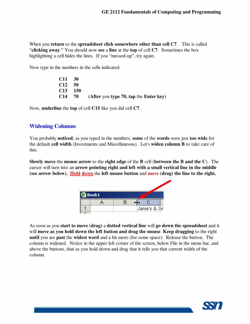
You probably noticed, as you typed in the numbers, some of the words were just too wide for
the default cell width (Investments and Miscellaneous). Let's widen column B to take care of this.
Slowly move the mouse arrow to the right edge of the B cell (between the B and the C). The
cursor will turn into an arrow pointing right and left with a small vertical line in the middle
(see arrow below). Hold down the left mouse button and move (drag) the line to the right.
As soon as you start to move (drag) a dotted vertical line will go down the spreadsheet and it
will move as you hold down the left button and drag the mouse. Keep dragging to the right
until you are past the widest word and a bit more (for some space). Release the button. The column is widened. Notice in the upper left corner of the screen, below File in the menu bar, and above the buttons, that as you hold down and drag that it tells you that current width of the column.
GE 2112 Fundamentals of Computing and Programming
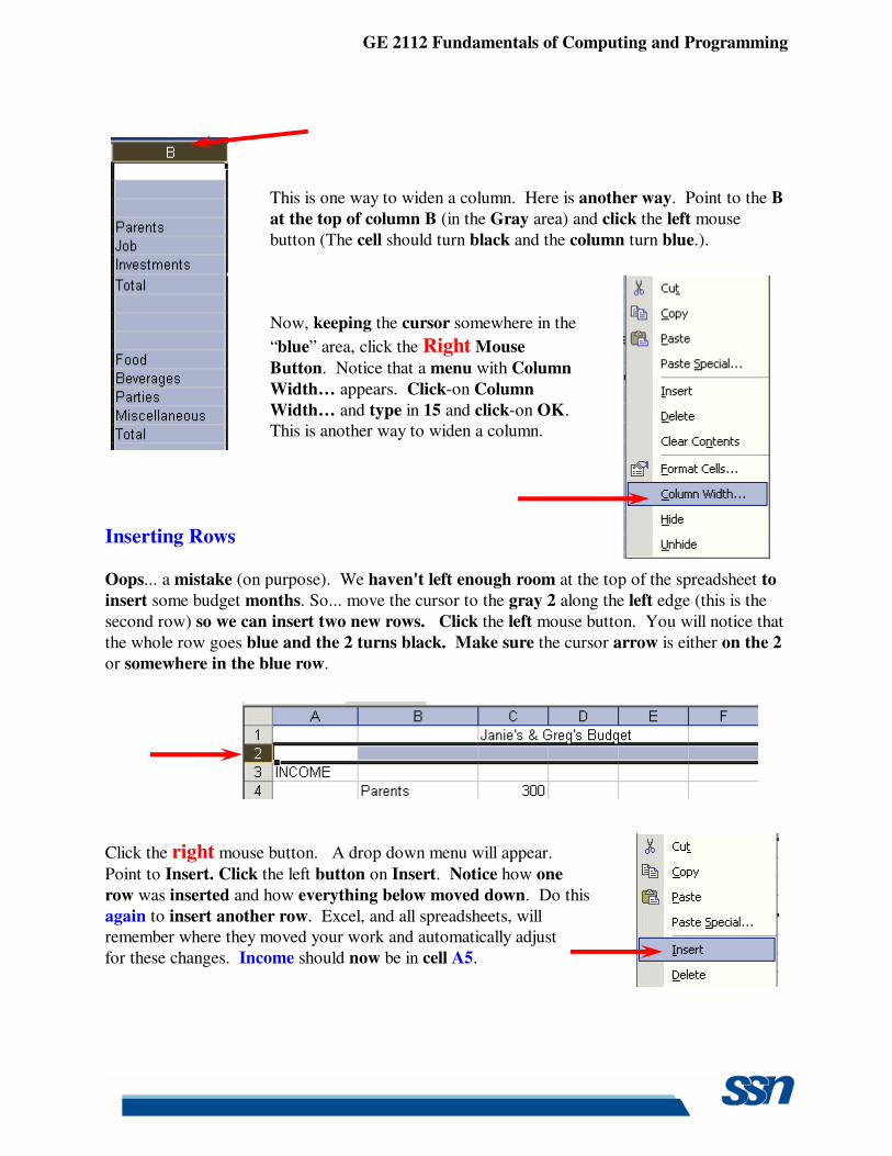
This is one way to widen a column. Here is another way. Point to the B
at the top of column B (in the Gray area) and click the left mouse
button (The cell should turn black and the column turn blue.).
Now, keeping the cursor somewhere in the
“blue” area, click the Right Mouse
Button. Notice that a menu with Column
Width… appears. Click-on Column
Width… and type in 15 and click-on OK. This is another way to widen a column.
Inserting Rows
Oops... a mistake (on purpose). We haven't left enough room at the top of the spreadsheet to
insert some budget months. So... move the cursor to the gray 2 along the left edge (this is the
second row) so we can insert two new rows. Click the left mouse button. You will notice that
the whole row goes blue and the 2 turns black. Make sure the cursor arrow is either on the 2
or somewhere in the blue row.
Click the right mouse button. A drop down menu will appear.
Point to Insert. Click the left button on Insert. Notice how one
row was inserted and how everything below moved down. Do this
again to insert another row. Excel, and all spreadsheets, will remember where they moved your work and automatically adjust
for these changes. Income should now be in cell A5.
GE 2112 Fundamentals of Computing and Programming
Aligning Cells
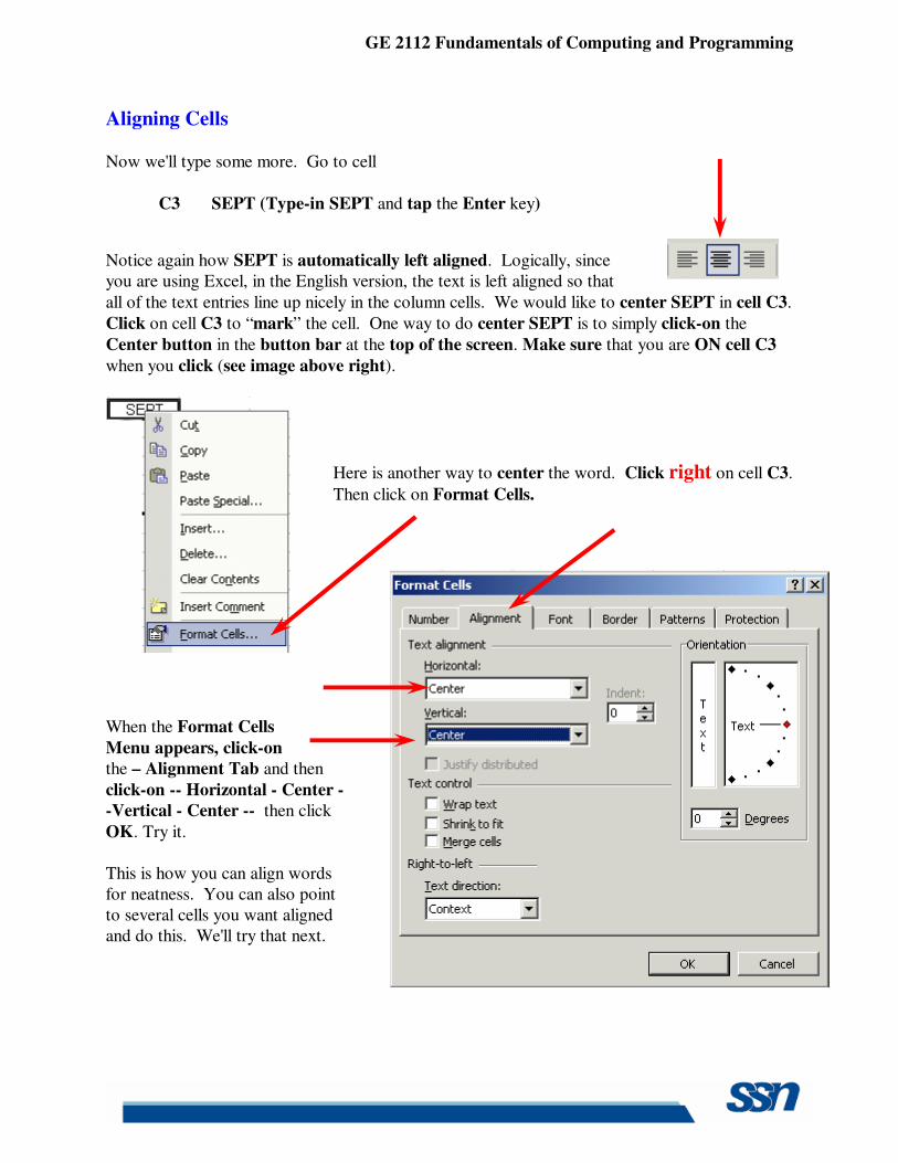
Now we'll type some more. Go to cell
C3 SEPT (Type-in SEPT and tap the Enter key)
Notice again how SEPT is automatically left aligned. Logically, since you are using Excel, in the English version, the text is left aligned so that
all of the text entries line up nicely in the column cells. We would like to center SEPT in cell C3.
Click on cell C3 to “mark” the cell. One way to do center SEPT is to simply click-on the
Center button in the button bar at the top of the screen. Make sure that you are ON cell C3
when you click (see image above right).
Here is another way to center the word. Click right on cell C3.
Then click on Format Cells.
When the Format Cells
Menu appears, click-on the – Alignment Tab and then
click-on -- Horizontal - Center --Vertical - Center -- then click
OK. Try it. This is how you can align words for neatness. You can also point to several cells you want aligned and do this. We'll try that next.
GE 2112 Fundamentals of Computing and Programming
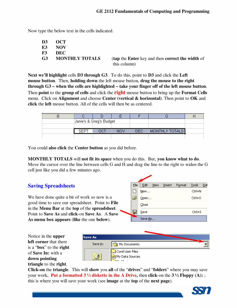
Now type the below text in the cells indicated.
D3 OCT E3 NOV F3 DEC
G3 MONTHLY TOTALS (tap the Enter key and then correct the width of this column)
Next we’ll highlight cells D3 through G3. To do this, point to D3 and click the Left
mouse button. Then, holding down the left mouse button, drag the mouse to the right
through G3 – when the cells are highlighted – take your finger off of the left mouse button.
Then point to the group of cells and click the right mouse button to bring up the Format Cells
menu. Click on Alignment and choose Center (vertical & horizontal). Then point to OK and
click the left mouse button. All of the cells will then be as centered.
You could also click the Center button as you did before.
MONTHLY TOTALS will not fit its space when you do this. But, you know what to do. Move the cursor over the line between cells G and H and drag the line to the right to widen the G cell just like you did a few minutes ago.
Saving Spreadsheets
We have done quite a bit of work so now is a
good time to save our spreadsheet. Point to File
in the Menu Bar at the top of the spreadsheet.
Point to Save As and click-on Save As. A Save
As menu box appears (like the one below).
Notice in the upper
left corner that there
is a “box” to the right
of Save In: with a
down pointing triangle to the right.
Click-on the triangle. This will show you all of the “drives” and “folders” where you may save
your work. Put a formatted 3 ½ diskette in the A Drive, then click-on the 3 ½ Floppy (A): ;
this is where you will save your work (see image at the top of the next page).
GE 2112 Fundamentals of Computing and Programming
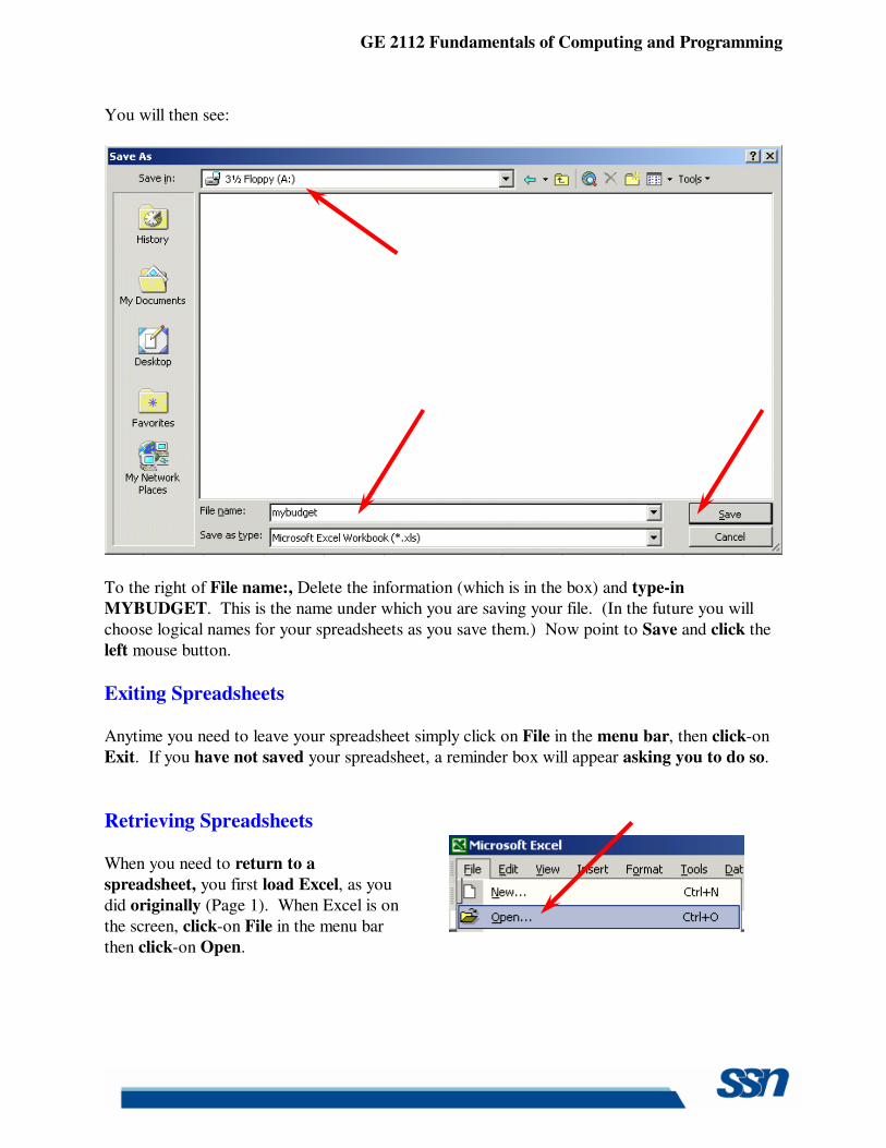
You will then see:
To the right of File name:, Delete the information (which is in the box) and type-in
MYBUDGET. This is the name under which you are saving your file. (In the future you will
choose logical names for your spreadsheets as you save them.) Now point to Save and click the
left mouse button.
Exiting Spreadsheets Anytime you need to leave your spreadsheet simply click on File in the menu bar, then click-on
Exit. If you have not saved your spreadsheet, a reminder box will appear asking you to do so.
Retrieving Spreadsheets When you need to return to a
spreadsheet, you first load Excel, as you
did originally (Page 1). When Excel is on
the screen, click-on File in the menu bar
then click-on Open.
GE 2112 Fundamentals of Computing and Programming
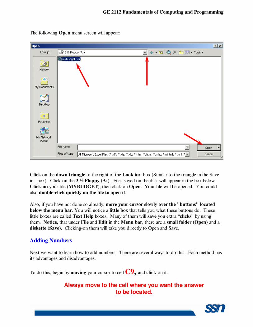
The following Open menu screen will appear:
Click on the down triangle to the right of the Look in: box (Similar to the triangle in the Save
in: box). Click-on the 3 ½ Floppy (A:). Files saved on the disk will appear in the box below.
Click-on your file (MYBUDGET), then click-on Open. Your file will be opened. You could
also double-click quickly on the file to open it.
Also, if you have not done so already, move your cursor slowly over the "buttons" located
below the menu bar. You will notice a little box that tells you what these buttons do. These
little boxes are called Text Help boxes. Many of them will save you extra “clicks” by using
them. Notice, that under File and Edit in the Menu bar, there are a small folder (Open) and a
diskette (Save). Clicking-on them will take you directly to Open and Save.
Adding Numbers Next we want to learn how to add numbers. There are several ways to do this. Each method has its advantages and disadvantages.
To do this, begin by moving your cursor to cell C9, and click-on it.
Always move to the cell where you want the answer to be located.
GE 2112 Fundamentals of Computing and Programming
TYPE-IN METHOD
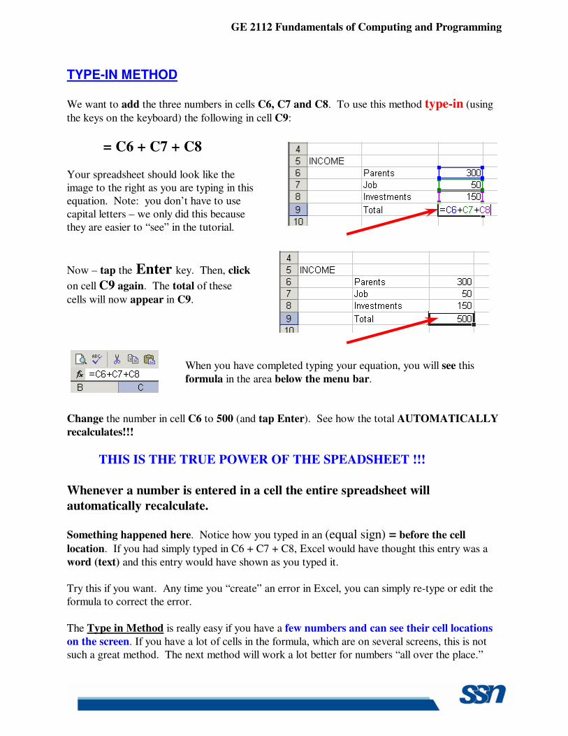
We want to add the three numbers in cells C6, C7 and C8. To use this method type-in (using
the keys on the keyboard) the following in cell C9:
= C6 + C7 + C8 Your spreadsheet should look like the image to the right as you are typing in this equation. Note: you don’t have to use capital letters – we only did this because they are easier to “see” in the tutorial.
Now – tap the Enter key. Then, click
on cell C9 again. The total of these
cells will now appear in C9.
When you have completed typing your equation, you will see this
formula in the area below the menu bar.
Change the number in cell C6 to 500 (and tap Enter). See how the total AUTOMATICALLY
recalculates!!!
THIS IS THE TRUE POWER OF THE SPEADSHEET !!! Whenever a number is entered in a cell the entire spreadsheet will automatically recalculate.
Something happened here. Notice how you typed in an (equal sign) = before the cell
location. If you had simply typed in C6 + C7 + C8, Excel would have thought this entry was a
word (text) and this entry would have shown as you typed it. Try this if you want. Any time you “create” an error in Excel, you can simply re-type or edit the formula to correct the error.
The Type in Method is really easy if you have a few numbers and can see their cell locations
on the screen. If you have a lot of cells in the formula, which are on several screens, this is not such a great method. The next method will work a lot better for numbers “all over the place.”
GE 2112 Fundamentals of Computing and Programming
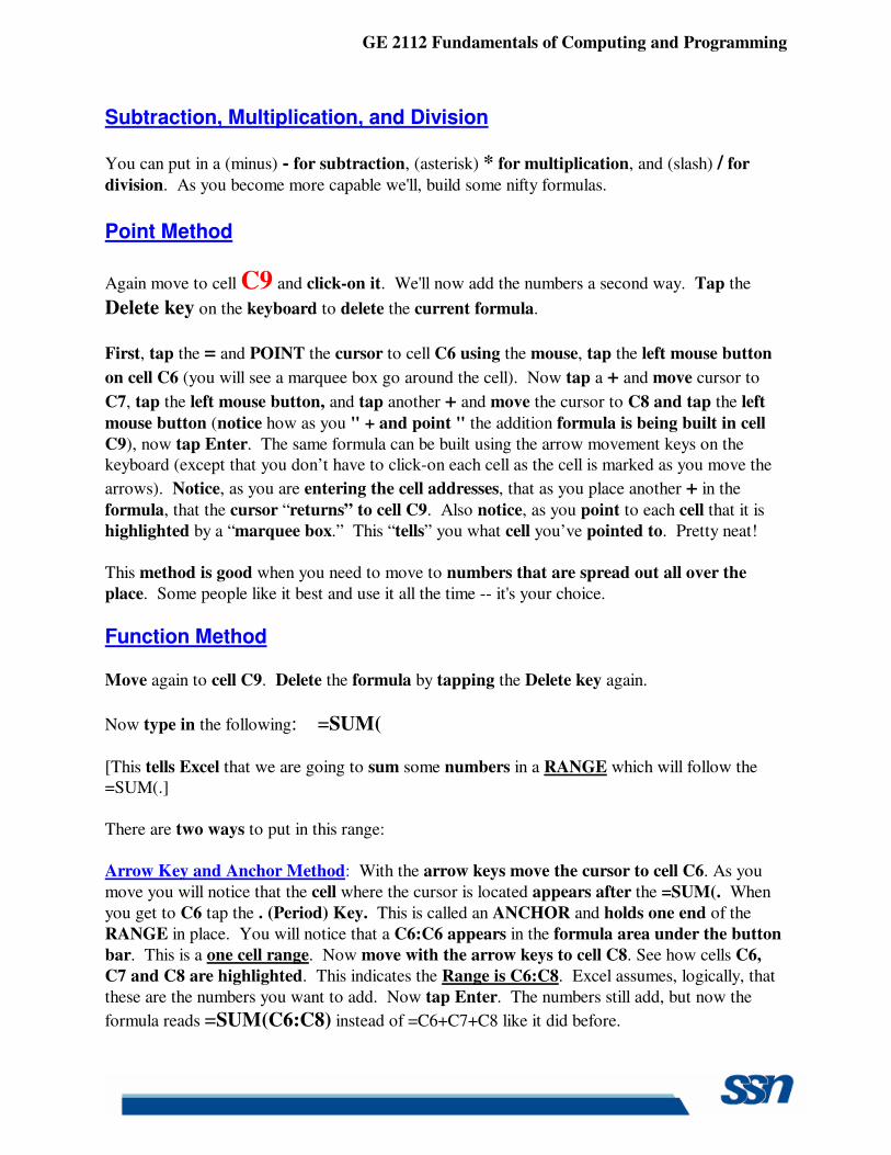
Subtraction, Multiplication, and Division
You can put in a (minus) - for subtraction, (asterisk) * for multiplication, and (slash) / for
division. As you become more capable we'll, build some nifty formulas.
Point Method
Again move to cell C9 and click-on it. We'll now add the numbers a second way. Tap the
Delete key on the keyboard to delete the current formula.
First, tap the = and POINT the cursor to cell C6 using the mouse, tap the left mouse button
on cell C6 (you will see a marquee box go around the cell). Now tap a + and move cursor to
C7, tap the left mouse button, and tap another + and move the cursor to C8 and tap the left
mouse button (notice how as you " + and point " the addition formula is being built in cell
C9), now tap Enter. The same formula can be built using the arrow movement keys on the keyboard (except that you don’t have to click-on each cell as the cell is marked as you move the
arrows). Notice, as you are entering the cell addresses, that as you place another + in the
formula, that the cursor “returns” to cell C9. Also notice, as you point to each cell that it is
highlighted by a “marquee box.” This “tells” you what cell you’ve pointed to. Pretty neat!
This method is good when you need to move to numbers that are spread out all over the
place. Some people like it best and use it all the time -- it's your choice.
Function Method Move again to cell C9. Delete the formula by tapping the Delete key again.
Now type in the following: =SUM(
[This tells Excel that we are going to sum some numbers in a RANGE which will follow the =SUM(.]
There are two ways to put in this range:
Arrow Key and Anchor Method: With the arrow keys move the cursor to cell C6. As you
move you will notice that the cell where the cursor is located appears after the =SUM(. When
you get to C6 tap the . (Period) Key. This is called an ANCHOR and holds one end of the
RANGE in place. You will notice that a C6:C6 appears in the formula area under the button
bar. This is a one cell range. Now move with the arrow keys to cell C8. See how cells C6,
C7 and C8 are highlighted. This indicates the Range is C6:C8. Excel assumes, logically, that
these are the numbers you want to add. Now tap Enter. The numbers still add, but now the
formula reads =SUM(C6:C8) instead of =C6+C7+C8 like it did before.
GE 2112 Fundamentals of Computing and Programming
Mouse Method: Move again to cell C9. Delete the formula in cell C9 by tapping the Delete
key. Type in =SUM( as you did before. Point to Cell C6 – with your mouse cursor. Click
and hold down the left mouse button and move/drag the cursor down to cell C8. (Cells C6,
C7 and C8 should be highlighted.) Now tap Enter.
This =SUM Function is a great way to add a lot of numbers, or a block/range of numbers. By simply anchoring, and using page downs or using the mouse, you can highlight lots and lots of numbers to add quickly. However, since it only sums you can't do subtraction, etc.
Point to cell C9 again. Tap the Delete key to remove the formula currently in cell C9.
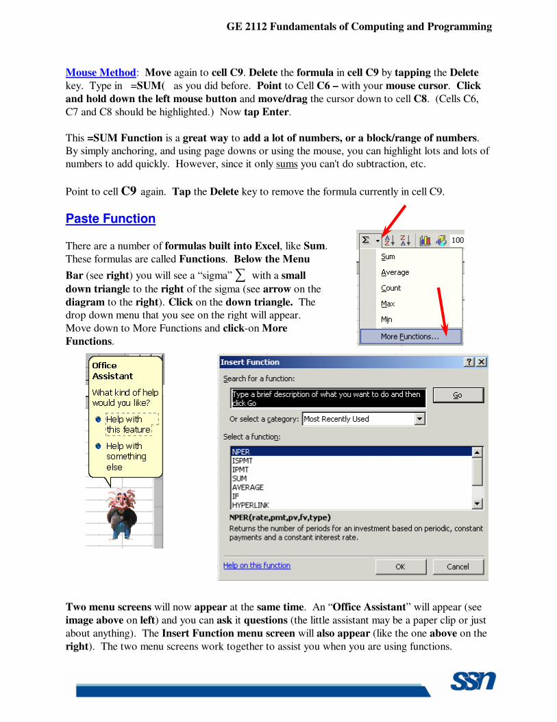
Paste Function
There are a number of formulas built into Excel, like Sum.
These formulas are called Functions. Below the Menu
Bar (see right) you will see a “sigma” ∑ with a small
down triangle to the right of the sigma (see arrow on the
diagram to the right). Click on the down triangle. The drop down menu that you see on the right will appear.
Move down to More Functions and click-on More
Functions.
Two menu screens will now appear at the same time. An “Office Assistant” will appear (see
image above on left) and you can ask it questions (the little assistant may be a paper clip or just
about anything). The Insert Function menu screen will also appear (like the one above on the
right). The two menu screens work together to assist you when you are using functions.
GE 2112 Fundamentals of Computing and Programming
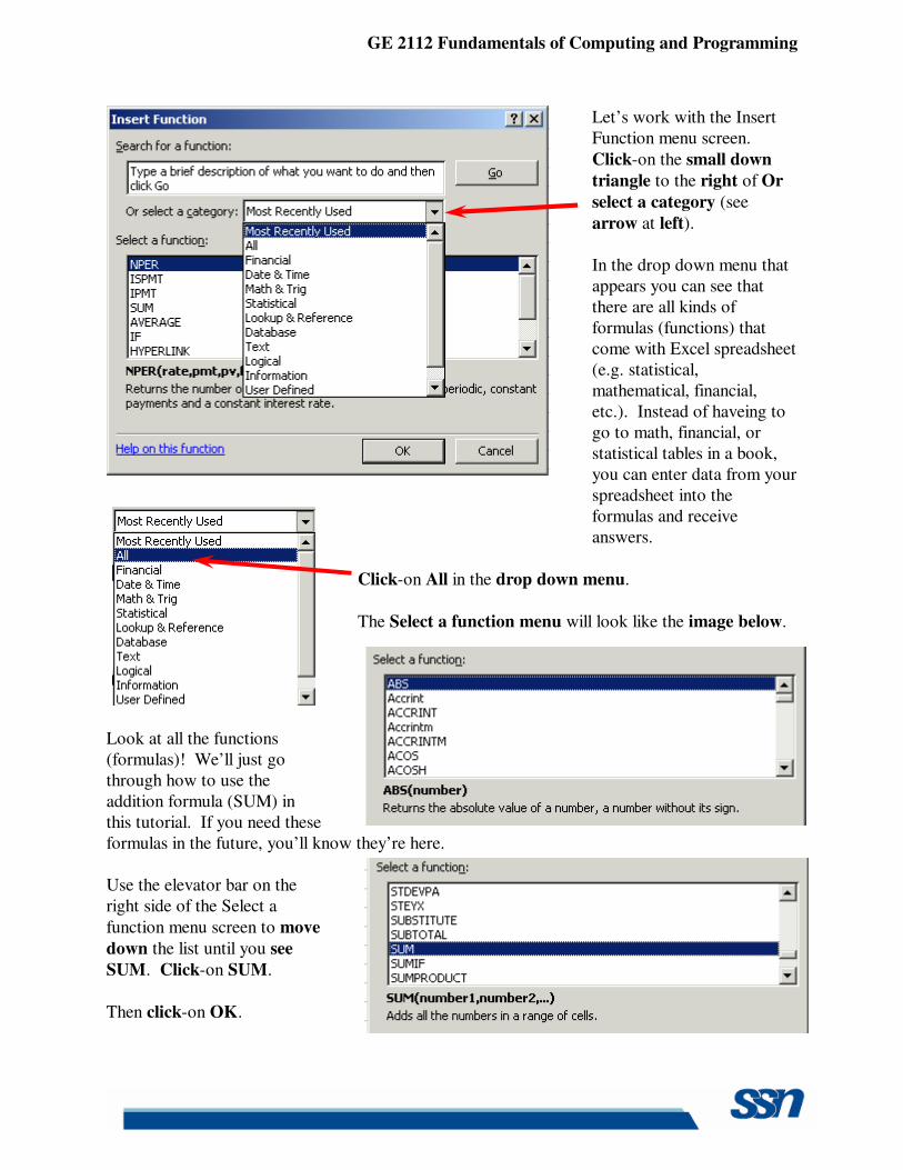
Let’s work with the Insert Function menu screen.
Click-on the small down
triangle to the right of Or
select a category (see
arrow at left). In the drop down menu that appears you can see that there are all kinds of formulas (functions) that come with Excel spreadsheet (e.g. statistical, mathematical, financial, etc.). Instead of haveing to go to math, financial, or statistical tables in a book, you can enter data from your spreadsheet into the formulas and receive answers.
Click-on All in the drop down menu.
The Select a function menu will look like the image below.
Look at all the functions (formulas)! We’ll just go through how to use the addition formula (SUM) in this tutorial. If you need these formulas in the future, you’ll know they’re here. Use the elevator bar on the right side of the Select a
function menu screen to move
down the list until you see
SUM. Click-on SUM.
Then click-on OK.
GE 2112 Fundamentals of Computing and Programming
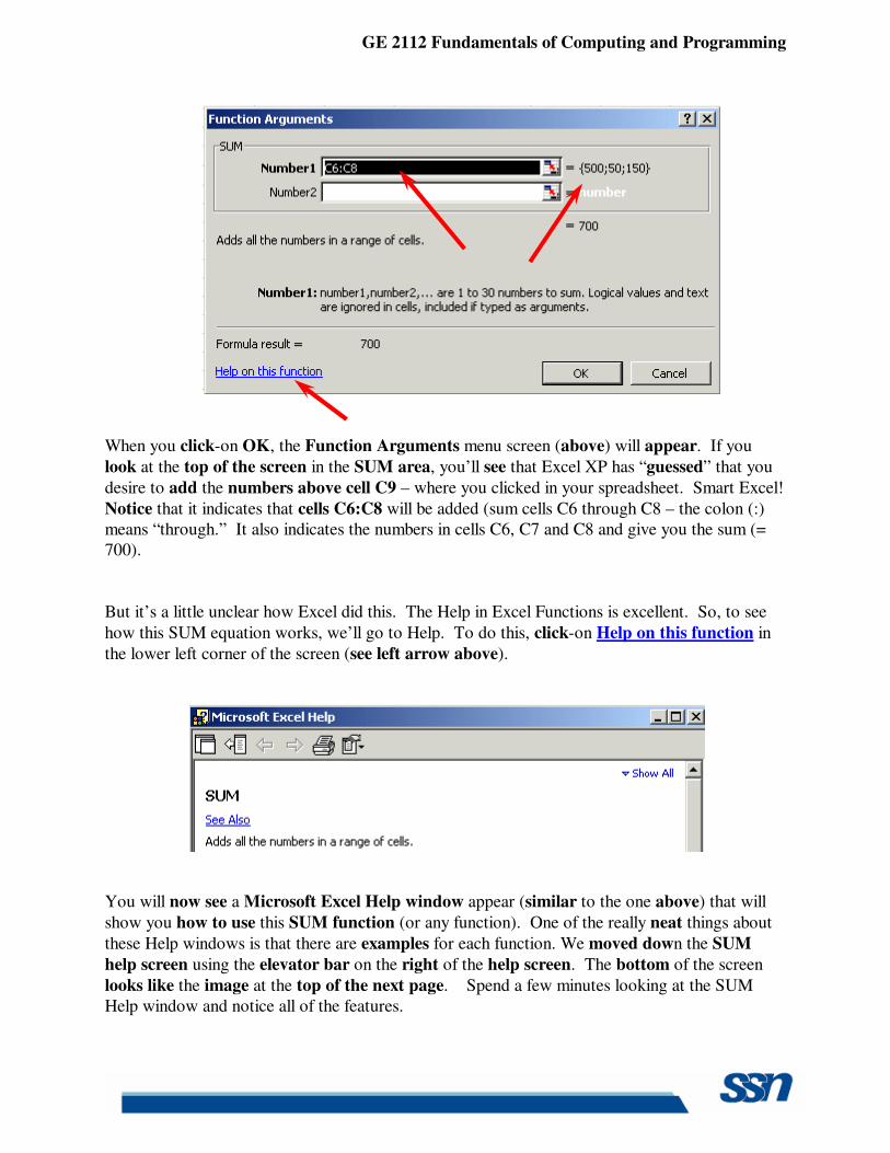
When you click-on OK, the Function Arguments menu screen (above) will appear. If you
look at the top of the screen in the SUM area, you’ll see that Excel XP has “guessed” that you
desire to add the numbers above cell C9 – where you clicked in your spreadsheet. Smart Excel!
Notice that it indicates that cells C6:C8 will be added (sum cells C6 through C8 – the colon (:) means “through.” It also indicates the numbers in cells C6, C7 and C8 and give you the sum (= 700). But it’s a little unclear how Excel did this. The Help in Excel Functions is excellent. So, to see
how this SUM equation works, we’ll go to Help. To do this, click-on Help on this function in
the lower left corner of the screen (see left arrow above).
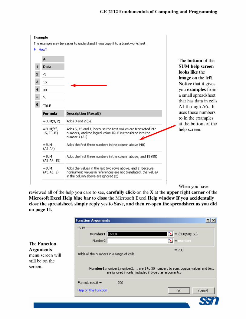
You will now see a Microsoft Excel Help window appear (similar to the one above) that will
show you how to use this SUM function (or any function). One of the really neat things about
these Help windows is that there are examples for each function. We moved down the SUM
help screen using the elevator bar on the right of the help screen. The bottom of the screen
looks like the image at the top of the next page. Spend a few minutes looking at the SUM Help window and notice all of the features.
GE 2112 Fundamentals of Computing and Programming
The bottom of the
SUM help screen looks like the
image on the left.
Notice that it gives
you examples from a small spreadsheet that has data in cells A1 through A6. It uses these numbers to in the examples at the bottom of the help screen. When you have
reviewed all of the help you care to see, carefully click-on the X at the upper right corner of the
Microsoft Excel Help blue bar to close the Microsoft Excel Help window If you accidentally
close the spreadsheet, simply reply yes to Save, and then re-open the spreadsheet as you did on page 11.
The Function
Arguments menu screen will still be on the screen.
GE 2112 Fundamentals of Computing and Programming
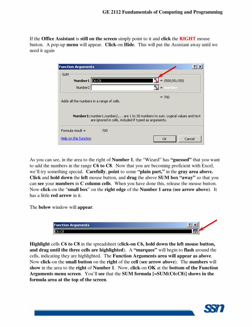
If the Office Assistant is still on the screen simply point to it and click the RIGHT mouse
button. A pop-up menu will appear. Click-on Hide. This will put the Assistant away until we need it again
As you can see, in the area to the right of Number 1, the “Wizard” has “guessed” that you want
to add the numbers in the range C6 to C8. Now that you are becoming proficient with Excel,
we’ll try something special. Carefully, point to some “plain part,” in the gray area above.
Click and hold down the left mouse button, and drag the above SUM box “away” so that you
can see your numbers in C column cells. When you have done this, release the mouse button.
Now click-on the “small box” on the right edge of the Number 1 area (see arrow above). It
has a little red arrow in it.
The below window will appear.
Highlight cells C6 to C8 in the spreadsheet (click-on C6, hold down the left mouse button,
and drag until the three cells are highlighted). A “marquee” will begin to flash around the
cells, indicating they are highlighted. The Function Arguments area will appear as above.
Now click-on the small button on the right of the cell (see arrow above). The numbers will
show in the area to the right of Number 1. Now, click-on OK at the bottom of the Function
Arguments menu screen. You’ll see that the SUM formula [=SUM(C6:C8)] shows in the
formula area at the top of the screen.
GE 2112 Fundamentals of Computing and Programming
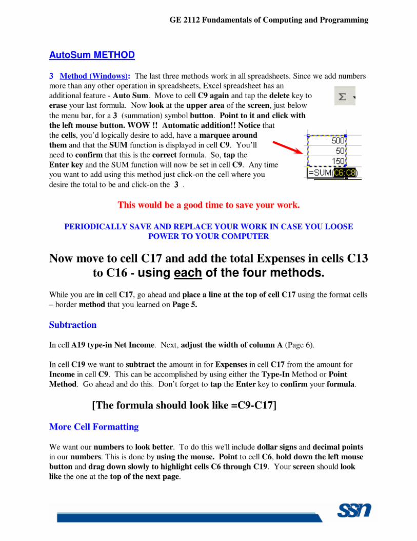
AutoSum METHOD
3333 Method (Windows): The last three methods work in all spreadsheets. Since we add numbers more than any other operation in spreadsheets, Excel spreadsheet has an
additional feature - Auto Sum. Move to cell C9 again and tap the delete key to
erase your last formula. Now look at the upper area of the screen, just below
the menu bar, for a 3333 (summation) symbol button. Point to it and click with
the left mouse button. WOW !! Automatic addition!! Notice that
the cells, you’d logically desire to add, have a marquee around
them and that the SUM function is displayed in cell C9. You’ll
need to confirm that this is the correct formula. So, tap the
Enter key and the SUM function will now be set in cell C9. Any time you want to add using this method just click-on the cell where you
desire the total to be and click-on the 3333 .
This would be a good time to save your work.
PERIODICALLY SAVE AND REPLACE YOUR WORK IN CASE YOU LOOSE POWER TO YOUR COMPUTER
Now move to cell C17 and add the total Expenses in cells C13 to C16 - using each of the four methods.
While you are in cell C17, go ahead and place a line at the top of cell C17 using the format cells
– border method that you learned on Page 5.
Subtraction
In cell A19 type-in Net Income. Next, adjust the width of column A (Page 6).
In cell C19 we want to subtract the amount in for Expenses in cell C17 from the amount for
Income in cell C9. This can be accomplished by using either the Type-In Method or Point
Method. Go ahead and do this. Don’t forget to tap the Enter key to confirm your formula.
[The formula should look like =C9-C17]
More Cell Formatting
We want our numbers to look better. To do this we'll include dollar signs and decimal points
in our numbers. This is done by using the mouse. Point to cell C6, hold down the left mouse
button and drag down slowly to highlight cells C6 through C19. Your screen should look
like the one at the top of the next page.
GE 2112 Fundamentals of Computing and Programming
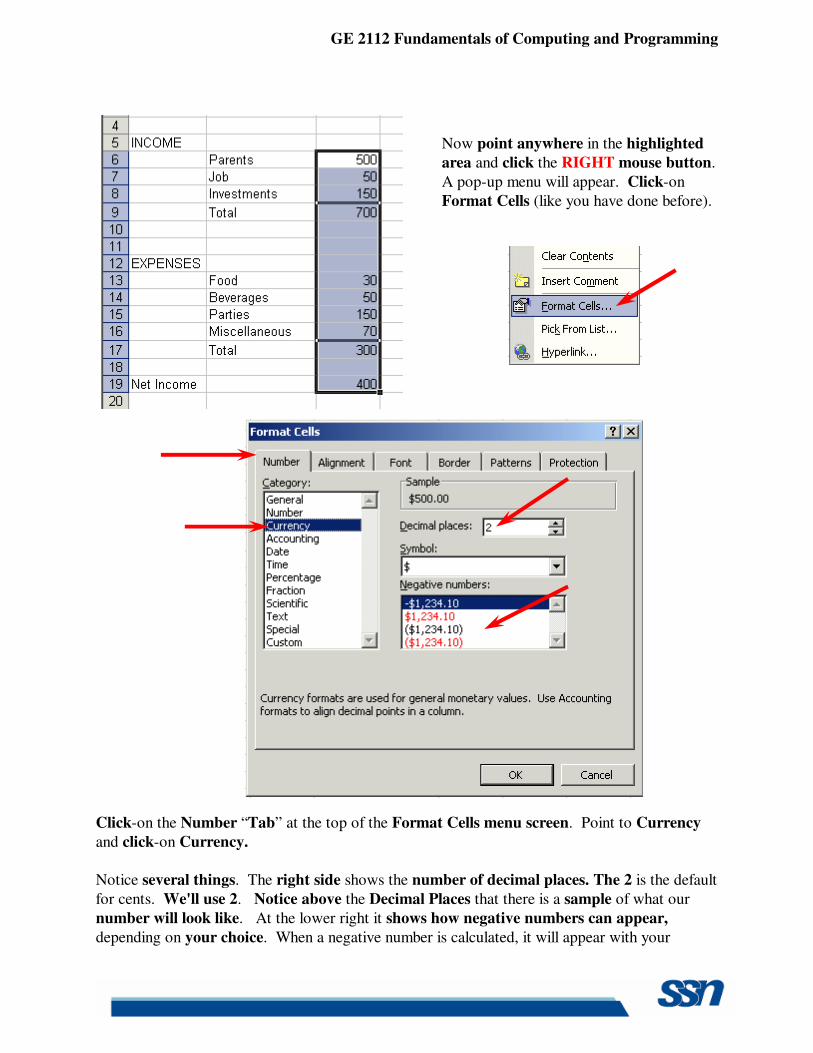
Now point anywhere in the highlighted
area and click the RIGHT mouse button.
A pop-up menu will appear. Click-on
Format Cells (like you have done before).
Click-on the Number “Tab” at the top of the Format Cells menu screen. Point to Currency
and click-on Currency.
Notice several things. The right side shows the number of decimal places. The 2 is the default
for cents. We'll use 2. Notice above the Decimal Places that there is a sample of what our
number will look like. At the lower right it shows how negative numbers can appear,
depending on your choice. When a negative number is calculated, it will appear with your
GE 2112 Fundamentals of Computing and Programming
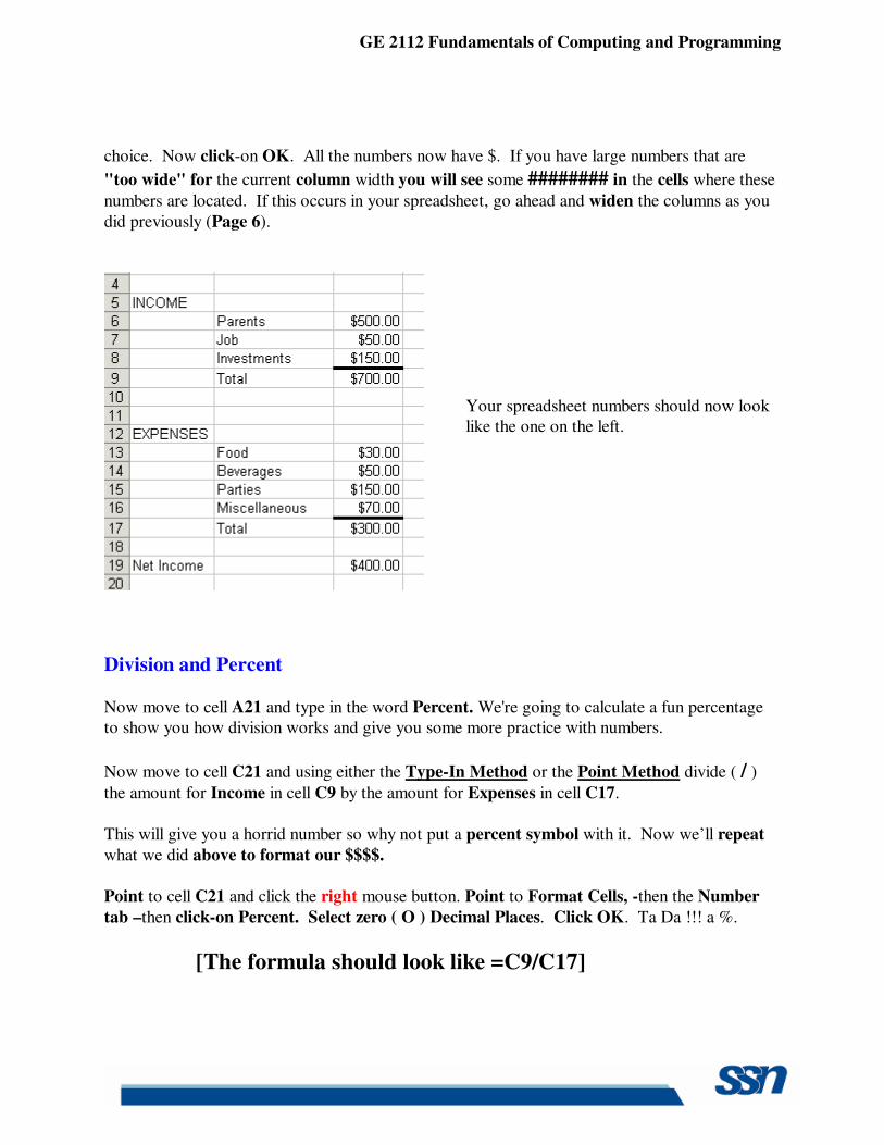
choice. Now click-on OK. All the numbers now have $. If you have large numbers that are
"too wide" for the current column width you will see some ######## in the cells where these
numbers are located. If this occurs in your spreadsheet, go ahead and widen the columns as you
did previously (Page 6).
Your spreadsheet numbers should now look like the one on the left.
Division and Percent
Now move to cell A21 and type in the word Percent. We're going to calculate a fun percentage to show you how division works and give you some more practice with numbers.
Now move to cell C21 and using either the Type-In Method or the Point Method divide ( / ) the amount for Income in cell C9 by the amount for Expenses in cell C17.
This will give you a horrid number so why not put a percent symbol with it. Now we’ll repeat
what we did above to format our $$$$.
Point to cell C21 and click the right mouse button. Point to Format Cells, -then the Number
tab –then click-on Percent. Select zero ( O ) Decimal Places. Click OK. Ta Da !!! a %.
[The formula should look like =C9/C17]
GE 2112 Fundamentals of Computing and Programming
Copying
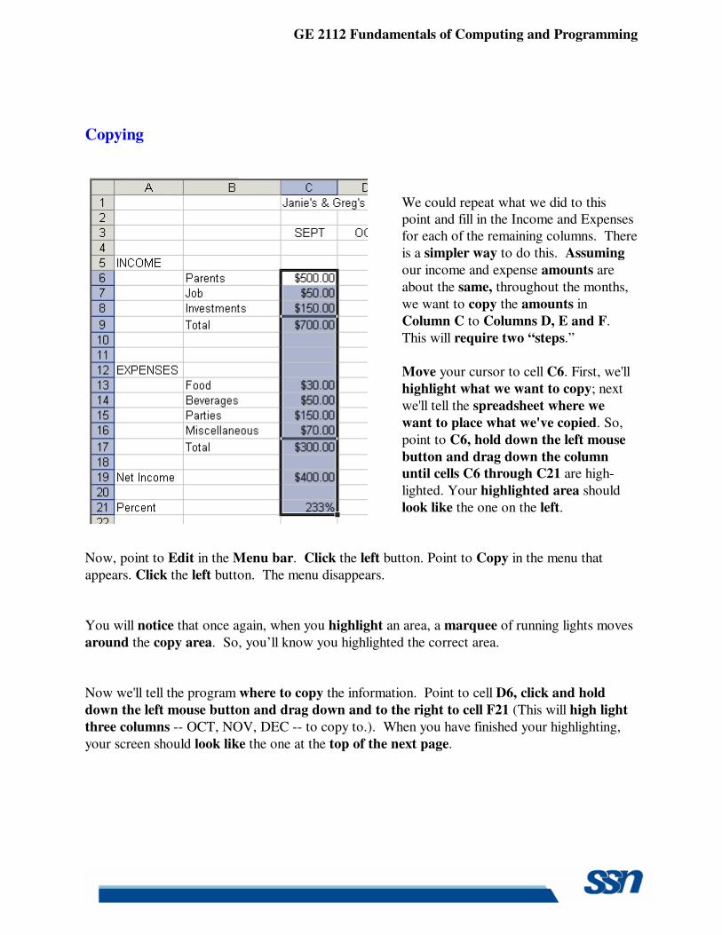
We could repeat what we did to this point and fill in the Income and Expenses for each of the remaining columns. There
is a simpler way to do this. Assuming
our income and expense amounts are
about the same, throughout the months,
we want to copy the amounts in
Column C to Columns D, E and F.
This will require two “steps.”
Move your cursor to cell C6. First, we'll
highlight what we want to copy; next
we'll tell the spreadsheet where we
want to place what we've copied. So,
point to C6, hold down the left mouse
button and drag down the column until cells C6 through C21 are high-
lighted. Your highlighted area should
look like the one on the left.
Now, point to Edit in the Menu bar. Click the left button. Point to Copy in the menu that
appears. Click the left button. The menu disappears.
You will notice that once again, when you highlight an area, a marquee of running lights moves
around the copy area. So, you’ll know you highlighted the correct area.
Now we'll tell the program where to copy the information. Point to cell D6, click and hold
down the left mouse button and drag down and to the right to cell F21 (This will high light
three columns -- OCT, NOV, DEC -- to copy to.). When you have finished your highlighting,
your screen should look like the one at the top of the next page.
GE 2112 Fundamentals of Computing and Programming
Now point to Edit in the Menu Bar again and click the left button. Point to Paste. Click left
button. Wow !' All those numbers and dollar signs and formulas - EVERYTHING - was
copied in a flash!! That sure saved us a lot of time. Click on a cell away from the area where the numbers are located. This will “turn-off” the
highlight. Tap the Esc key and the marquee will also disappear.
Note: You can also utilize the copy and paste buttons in the button bar to do this if you
desire. Change a few numbers in each of the months in both the income and expense areas to
see how the spreadsheet works. (This will be viewed in the graphs later.)
This would be a great time to Save again. Now for something to do on your own.
GE 2112 Fundamentals of Computing and Programming
Entering formulas in the Monthly Totals Column
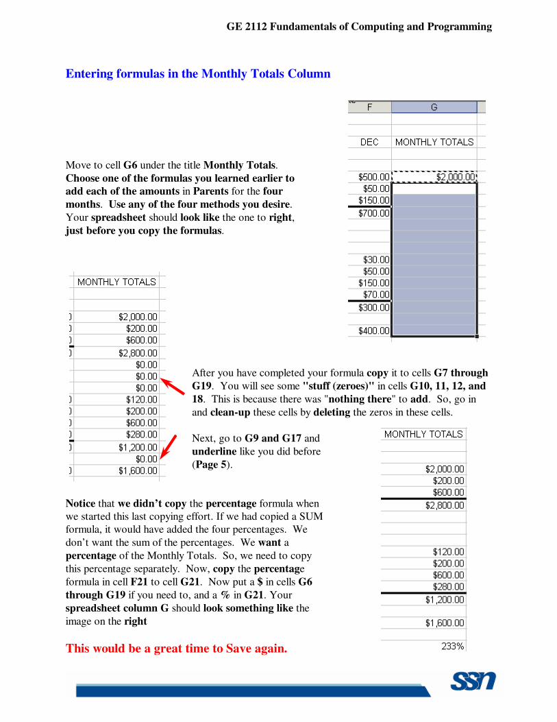
Move to cell G6 under the title Monthly Totals.
Choose one of the formulas you learned earlier to add each of the amounts in Parents for the four
months. Use any of the four methods you desire.
Your spreadsheet should look like the one to right,
just before you copy the formulas.
After you have completed your formula copy it to cells G7 through
G19. You will see some "stuff (zeroes)" in cells G10, 11, 12, and
18. This is because there was "nothing there" to add. So, go in
and clean-up these cells by deleting the zeros in these cells.
Next, go to G9 and G17 and
underline like you did before
(Page 5).
Notice that we didn’t copy the percentage formula when we started this last copying effort. If we had copied a SUM formula, it would have added the four percentages. We
don’t want the sum of the percentages. We want a
percentage of the Monthly Totals. So, we need to copy
this percentage separately. Now, copy the percentage
formula in cell F21 to cell G21. Now put a $ in cells G6
through G19 if you need to, and a % in G21. Your
spreadsheet column G should look something like the
image on the right
This would be a great time to Save again.
GE 2112 Fundamentals of Computing and Programming
Absoluting (and multiplication)
There are times, when we are working with a spreadsheet, that we do not want a cell to "roll"
to the next column when we use the copy feature of the spreadsheet – like it did in our last
copying exercise. To stop the cells from “rolling” we utilize something called absoluting. The following is an illustration of absoluting.
Go to cell A23 and type-in Number. Go to cell A25 and type-in Result.
Go to cell C23 and type in a 2 – and tap the Enter key.
We'll now create a formula to multiply our number times Net Income. You may use either the
Type-in or Point method. Go to cell C25, and type-in a formula to multiply cell C23 times cell
C19.
The formula should look like: =C23*C19
The result in C25 should be two times the net income in cell C19.
Now copy the formula in cell C25 to cells D25, E25, F25 and G25. Your row 25 should look
like the one below.
Uh Oh!!! Where did all of those "0's" come from?
Point to each of the cells D25, E25, F25 and G25. Notice, as you click on each and look at
the of the screen, how C23 (the cell with the 2) "rolled" and became D23, E23, F23 and G23
(which are blank - and caused the "0's"). A blank times a number is a “0.”We want the 2
to be in each formula and not to "roll".
To do this we utilize something called Absoluting or Anchoring.
Go back to cell C25. Now we'll enter the formula again, but a little differently
(to anchor the 2).
Type-in a =C23 (or you could type = and point to C23). NOW, tap the F4 key.
Notice, in the Edit bar at the top of the screen, that the =C23 changes to: $C$23. (This
tells you that cell C23 is absoluted or anchored. The "$'s" indicate the absoluting.) Now
finish the formula by typing in or pointing *C17 as before. Tap Enter.
The formula should look like: =$C$23*C19
GE 2112 Fundamentals of Computing and Programming
Now copy the formula in cell C25 to cells D25, E25, F25 and G25 again.
The numbers should now be correct. Point to cells D25, E25, F25 and G25 (like you did
before). You will notice the "$'s" have copied the =$C$23 to each cell (absoluting) and the Net Income figures have rolled as they should. Absoluting is something you should know and understand.
Pause and reflect -- Look at all you have accomplished. If you want go in and change some more numbers or change the income and expense titles to something you feel is more fun or appropriate.
This would be a great time to Save again.
The next important lesson to learn how to print. This done with a few easy steps.
Printing
First, move to cell A1.
All of the Windows spreadsheets try to figure out what you want to print. Sometimes they're right,
sometimes they're wrong. So........
The most important thing with printing is to tell the printer what to print.
Unlike a word processor, you may need to highlight what you want to print. For the moment, we’ll assume that Excel XP will “guess” correctly, and that you have not “clicked” somewhere that will cause a problem. If you do have problem, which we’ll know in a second, we’ll show you how to take care of the problem a bit later.
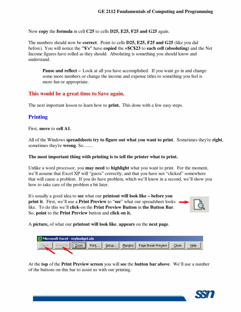
It's usually a good idea to see what our printout will look like – before you
print it. First, we’ll use a Print Preview to “see” what our spreadsheet looks
like. To do this we’ll click-on the Print Preview Button in the Button Bar.
So, point to the Print Preview button and click on it.
A picture, of what our printout will look like, appears on the next page.
At the top of the Print Preview screen you will see the button bar above. We’ll use a number of the buttons on this bar to assist us with our printing.
GE 2112 Fundamentals of Computing and Programming
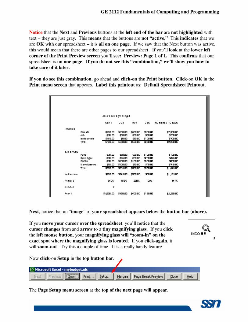
Notice that the Next and Previous buttons at the left end of the bar are not highlighted with
text – they are just gray. This means that the buttons are not “active.” This indicates that we
are OK with our spreadsheet – it is all on one page. If we saw that the Next button was active,
this would mean that there are other pages to our spreadsheet. If you’ll look at the lower left
corner of the Print Preview screen you’ll see: Preview: Page 1 of 1. This confirms that our
spreadsheet is on one page. If you do not see this “combination,” we’ll show you how to
take care of it later. If you do see this combination, go ahead and click-on the Print button. Click-on OK in the
Print menu screen that appears. Label this printout as: Default Spreadsheet Printout.
Next, notice that an “image” of your spreadsheet appears below the button bar (above).
If you move your cursor over the spreadsheet, you’ll notice that the
cursor changes from and arrow to a tiny magnifying glass. If you click
the left mouse button, your magnifying glass will “zoom-in” on the
exact spot where the magnifying glass is located. If you click-again, it
will zoom-out. Try this a couple of time. It is a really handy feature.
Now click-on Setup in the top button bar.
The Page Setup menu screen at the top of the next page will appear.
GE 2112 Fundamentals of Computing and Programming
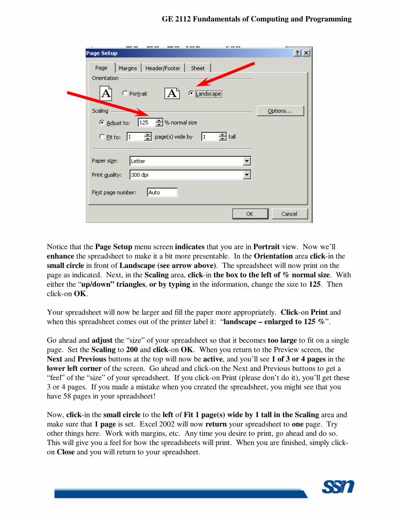
Notice that the Page Setup menu screen indicates that you are in Portrait view. Now we’ll
enhance the spreadsheet to make it a bit more presentable. In the Orientation area click-in the
small circle in front of Landscape (see arrow above). The spreadsheet will now print on the
page as indicated. Next, in the Scaling area, click-in the box to the left of % normal size. With
either the “up/down” triangles, or by typing in the information, change the size to 125. Then
click-on OK.
Your spreadsheet will now be larger and fill the paper more appropriately. Click-on Print and
when this spreadsheet comes out of the printer label it: “landscape – enlarged to 125 %”.
Go ahead and adjust the “size” of your spreadsheet so that it becomes too large to fit on a single
page. Set the Scaling to 200 and click-on OK. When you return to the Preview screen, the
Next and Previous buttons at the top will now be active, and you’ll see 1 of 3 or 4 pages in the
lower left corner of the screen. Go ahead and click-on the Next and Previous buttons to get a “feel” of the “size” of your spreadsheet. If you click-on Print (please don’t do it), you’ll get these 3 or 4 pages. If you made a mistake when you created the spreadsheet, you might see that you have 58 pages in your spreadsheet!
Now, click-in the small circle to the left of Fit 1 page(s) wide by 1 tall in the Scaling area and
make sure that 1 page is set. Excel 2002 will now return your spreadsheet to one page. Try other things here. Work with margins, etc. Any time you desire to print, go ahead and do so. This will give you a feel for how the spreadsheets will print. When you are finished, simply click-
on Close and you will return to your spreadsheet.
GE 2112 Fundamentals of Computing and Programming
Many folks ask how to center a spreadsheet on the page. This feature is located in Margins at the bottom of the screen. Simply click-on Margins at the top of the Preview screen or on the Margins tab when you are in the Setup screen.
Many folks also ask about how to place gridlines and show the row and column headings (A, B, C and 1, 2, 3) in their spreadsheet printouts. This feature is located on the Sheet tab in the Setup screen menu.
Cure for the problem – if you have too many spreadsheet pages.
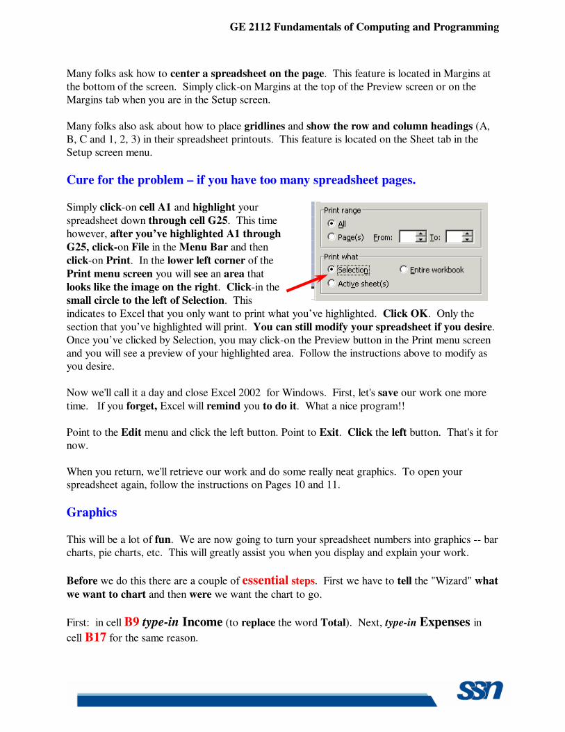
Simply click-on cell A1 and highlight your
spreadsheet down through cell G25. This time
however, after you’ve highlighted A1 through
G25, click-on File in the Menu Bar and then
click-on Print. In the lower left corner of the
Print menu screen you will see an area that
looks like the image on the right. Click-in the
small circle to the left of Selection. This
indicates to Excel that you only want to print what you’ve highlighted. Click OK. Only the
section that you’ve highlighted will print. You can still modify your spreadsheet if you desire. Once you’ve clicked by Selection, you may click-on the Preview button in the Print menu screen and you will see a preview of your highlighted area. Follow the instructions above to modify as you desire.
Now we'll call it a day and close Excel 2002 for Windows. First, let's save our work one more
time. If you forget, Excel will remind you to do it. What a nice program!!
Point to the Edit menu and click the left button. Point to Exit. Click the left button. That's it for now. When you return, we'll retrieve our work and do some really neat graphics. To open your spreadsheet again, follow the instructions on Pages 10 and 11.
Graphics This will be a lot of fun. We are now going to turn your spreadsheet numbers into graphics -- bar charts, pie charts, etc. This will greatly assist you when you display and explain your work.
Before we do this there are a couple of essential steps. First we have to tell the "Wizard" what
we want to chart and then were we want the chart to go.
First: in cell B9 type-in Income (to replace the word Total). Next, type-in Expenses in cell B17 for the same reason.
GE 2112 Fundamentals of Computing and Programming
VERY IMPORTANT……….
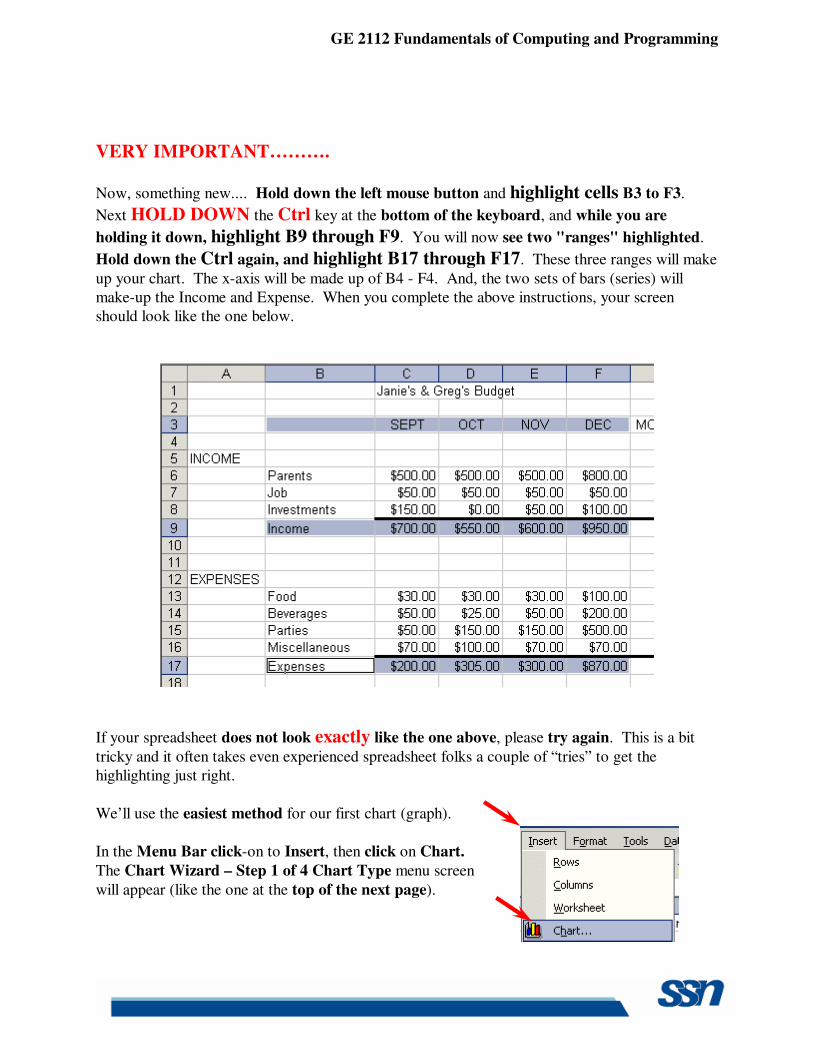
Now, something new.... Hold down the left mouse button and highlight cells B3 to F3.
Next HOLD DOWN the Ctrl key at the bottom of the keyboard, and while you are
holding it down, highlight B9 through F9. You will now see two "ranges" highlighted.
Hold down the Ctrl again, and highlight B17 through F17. These three ranges will make
up your chart. The x-axis will be made up of B4 - F4. And, the two sets of bars (series) will make-up the Income and Expense. When you complete the above instructions, your screen should look like the one below.
If your spreadsheet does not look exactly like the one above, please try again. This is a bit
tricky and it often takes even experienced spreadsheet folks a couple of “tries” to get the highlighting just right.
We’ll use the easiest method for our first chart (graph).
In the Menu Bar click-on to Insert, then click on Chart.
The Chart Wizard – Step 1 of 4 Chart Type menu screen
will appear (like the one at the top of the next page).
GE 2112 Fundamentals of Computing and Programming
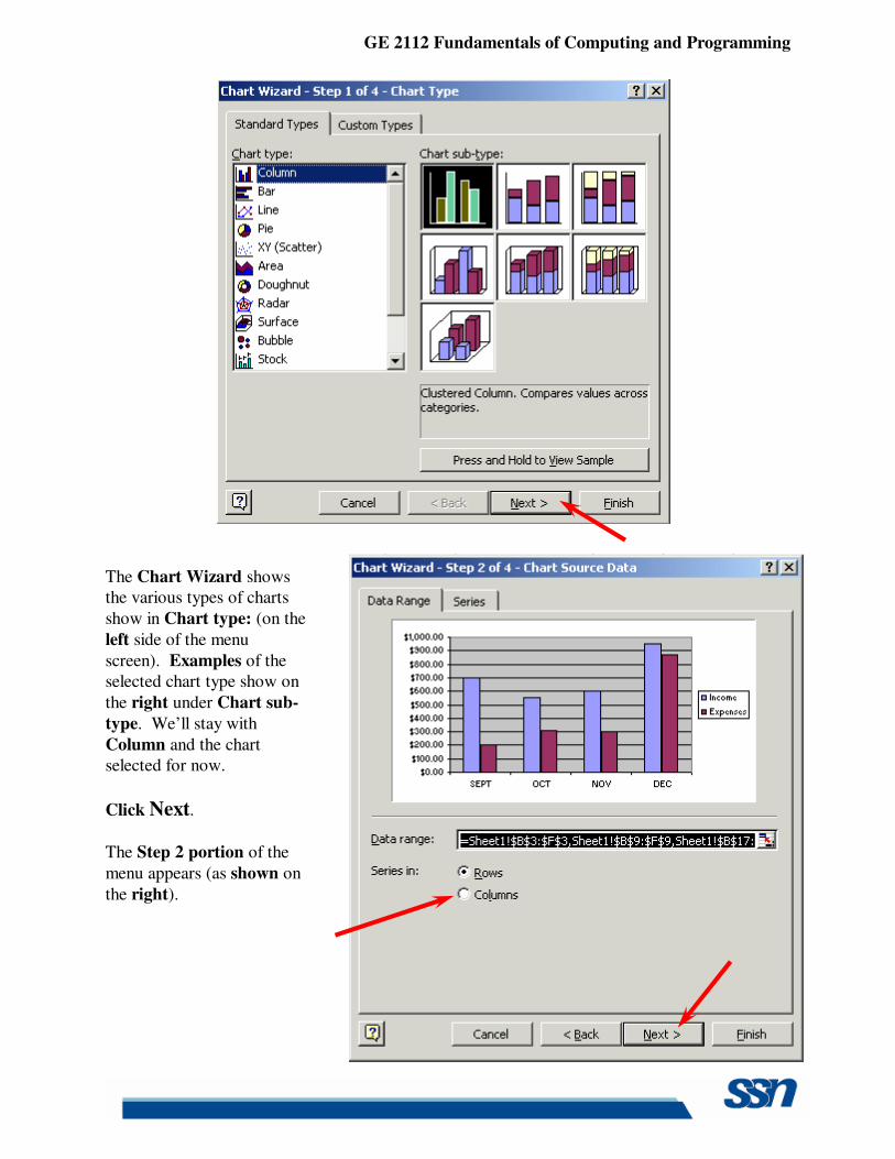
The Chart Wizard shows the various types of charts
show in Chart type: (on the
left side of the menu
screen). Examples of the selected chart type show on
the right under Chart sub-
type. We’ll stay with
Column and the chart selected for now.
Click Next.
The Step 2 portion of the
menu appears (as shown on
the right).
GE 2112 Fundamentals of Computing and Programming
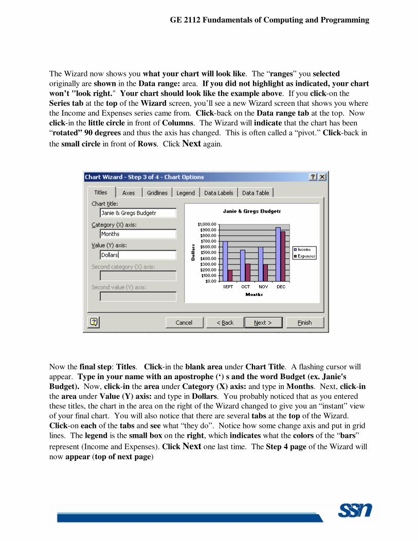
The Wizard now shows you what your chart will look like. The “ranges” you selected
originally are shown in the Data range: area. If you did not highlight as indicated, your chart
won’t "look right." Your chart should look like the example above. If you click-on the
Series tab at the top of the Wizard screen, you’ll see a new Wizard screen that shows you where
the Income and Expenses series came from. Click-back on the Data range tab at the top. Now
click-in the little circle in front of Columns. The Wizard will indicate that the chart has been
“rotated” 90 degrees and thus the axis has changed. This is often called a “pivot.” Click-back in
the small circle in front of Rows. Click Next again.
Now the final step: Titles. Click-in the blank area under Chart Title. A flashing cursor will
appear. Type in your name with an apostrophe (‘) s and the word Budget (ex. Janie's
Budget). Now, click-in the area under Category (X) axis: and type in Months. Next, click-in
the area under Value (Y) axis: and type in Dollars. You probably noticed that as you entered these titles, the chart in the area on the right of the Wizard changed to give you an “instant” view
of your final chart. You will also notice that there are several tabs at the top of the Wizard.
Click-on each of the tabs and see what “they do”. Notice how some change axis and put in grid
lines. The legend is the small box on the right, which indicates what the colors of the “bars”
represent (Income and Expenses). Click Next one last time. The Step 4 page of the Wizard will
now appear (top of next page)
GE 2112 Fundamentals of Computing and Programming
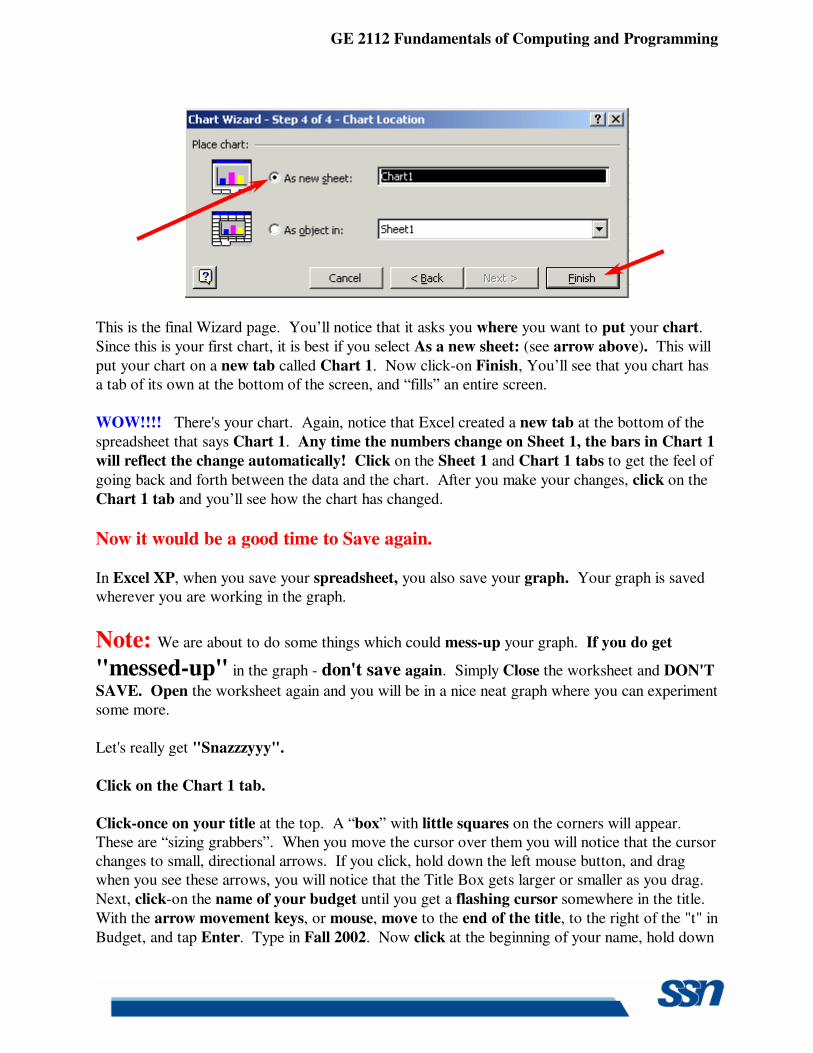
This is the final Wizard page. You’ll notice that it asks you where you want to put your chart.
Since this is your first chart, it is best if you select As a new sheet: (see arrow above). This will
put your chart on a new tab called Chart 1. Now click-on Finish, You’ll see that you chart has a tab of its own at the bottom of the screen, and “fills” an entire screen.
WOW!!!! There's your chart. Again, notice that Excel created a new tab at the bottom of the
spreadsheet that says Chart 1. Any time the numbers change on Sheet 1, the bars in Chart 1
will reflect the change automatically! Click on the Sheet 1 and Chart 1 tabs to get the feel of
going back and forth between the data and the chart. After you make your changes, click on the
Chart 1 tab and you’ll see how the chart has changed.
Now it would be a good time to Save again.
In Excel XP, when you save your spreadsheet, you also save your graph. Your graph is saved wherever you are working in the graph.
Note: We are about to do some things which could mess-up your graph. If you do get
"messed-up" in the graph - don't save again. Simply Close the worksheet and DON'T
SAVE. Open the worksheet again and you will be in a nice neat graph where you can experiment some more.
Let's really get "Snazzzyyy".
Click on the Chart 1 tab. Click-once on your title at the top. A “box” with little squares on the corners will appear. These are “sizing grabbers”. When you move the cursor over them you will notice that the cursor changes to small, directional arrows. If you click, hold down the left mouse button, and drag when you see these arrows, you will notice that the Title Box gets larger or smaller as you drag.
Next, click-on the name of your budget until you get a flashing cursor somewhere in the title.
With the arrow movement keys, or mouse, move to the end of the title, to the right of the "t" in
Budget, and tap Enter. Type in Fall 2002. Now click at the beginning of your name, hold down
GE 2112 Fundamentals of Computing and Programming
the left mouse button, and drag to highlight the first line of the budget title with your name in
it. Keeping the cursor on the dark area, click the right mouse button. Click-on Format Chart
Title. Change the Font to Times New Roman (by moving up and down with the arrows). As
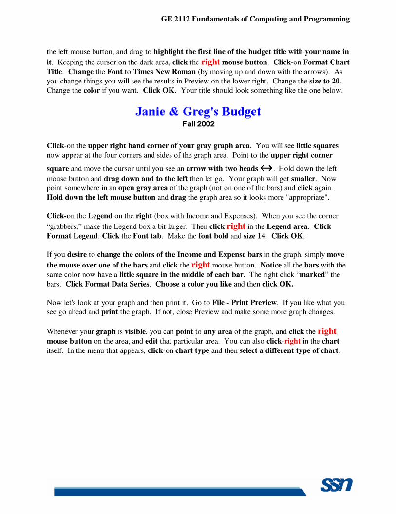
you change things you will see the results in Preview on the lower right. Change the size to 20.
Change the color if you want. Click OK. Your title should look something like the one below.
Click-on the upper right hand corner of your gray graph area. You will see little squares
now appear at the four corners and sides of the graph area. Point to the upper right corner
square and move the cursor until you see an arrow with two heads ↔↔↔↔ . Hold down the left
mouse button and drag down and to the left then let go. Your graph will get smaller. Now
point somewhere in an open gray area of the graph (not on one of the bars) and click again.
Hold down the left mouse button and drag the graph area so it looks more "appropriate".
Click-on the Legend on the right (box with Income and Expenses). When you see the corner
“grabbers,” make the Legend box a bit larger. Then click right in the Legend area. Click
Format Legend. Click the Font tab. Make the font bold and size 14. Click OK.
If you desire to change the colors of the Income and Expense bars in the graph, simply move
the mouse over one of the bars and click the right mouse button. Notice all the bars with the
same color now have a little square in the middle of each bar. The right click “marked” the
bars. Click Format Data Series. Choose a color you like and then click OK.
Now let's look at your graph and then print it. Go to File - Print Preview. If you like what you
see go ahead and print the graph. If not, close Preview and make some more graph changes.
Whenever your graph is visible, you can point to any area of the graph, and click the right mouse button on the area, and edit that particular area. You can also click-right in the chart
itself. In the menu that appears, click-on chart type and then select a different type of chart.


![Manual Excel Xp[1]](https://img.pdfslide.net/doc/110x75/5571f3d449795947648ea407/manual-excel-xp1.jpg)