Exchange rate effects: A case study of the export performance

of the Swiss Agriculture and Food Sector

Andreas Kohler and Ali Ferjani

Agroscope, Institute for Sustainability Sciences ISS, Switzerland

The Swiss franc appreciated strongly against the currencies of Switzerland’s most

important trading partners after the global financial crisis in 2008. This has led to

renewed interest in the question of how sensitive Swiss exports are with respect to

exchange rate movements. We analyze this question for exports of the Swiss Agriculture

and Food Sector, using both time series and dynamic panel data models based on data

from 1999 to 2012. We find that in the long-run a one percent appreciation of the

Swiss franc leads on average to a decrease in exports of agricultural and food products

of approximately 0.9 percent. Our results suggest that on average, producers in the

Swiss Agriculture and Food Sector are able to successfully avoid price competition by

differentiating their products, producing high-quality products for niche markets.

1 Introduction

Since the global financial crisis in 2008 the Swiss franc has appreciated strongly against thecurrencies of Switzerland’s major trading partners. During two years, from the onset of theglobal financial crisis in 2008 to the introduction of the exchange rate peg against the Euro bythe Swiss National Bank in September 2011, the Swiss franc appreciated about 25 percent(in real terms) against the currencies of Switzerland’s most important export markets foragriculture and food products, thus, potentially depressing foreign demand for Swiss products.At the same time, the Swiss Agriculture and Food Sector has become more integrated into theworld market. Against this backdrop, there has been renewed interest in the question of howchanges in the exchange rate affect exports in general, and exports of the Swiss Agricultureand Food Sector in particular.

The main contribution of this paper is to estimate and quantify the effects of exchangerate fluctuations on Swiss agro-food exports. The case study of the Swiss Agriculture andFood Sector has the following advantages. On the one hand, Switzerland is a small openeconomy, with an independent economic and monetary policy, which has lately experiencedsharp movements of its currency. On the other hand, the Agriculture and Food Sector isrelatively small compared to the rest of the Swiss economy, which has the advantage thata causal interpretation of the results becomes more plausible (in particular, we don’t haveto worry much about reverse causality).1 Hence, for policy makers this case study couldyield valuable insight into the reaction of exporters to exchange rate fluctuations under aparticular set of economic policies. We will see below that the behavior of exporters inother sectors of the Swiss economy is relatively similar. Thus, we think that the lessonslearned could be generalized to some extent to other sectors, as well as to other economiessimilar to Switzerland. Furthermore, we exploit time series as well as panel data to estimateexchange rate effects. The time series analysis has the advantage of a clear identificationstrategy since only variation over time is used to identify parameters but might suffer from alarge bias due to small sample size. The panel data analysis allows us to increase sample sizeand exploit the information contained in the cross-section, which might ameliorate potentialbias. The downside is that the estimated (dynamic) panel data models are sensitive to modelspecification (and the set of instruments). However, the analysis of both time series andpanel data helps us to assess the sensitivity of our results with respect to model specification,estimation methods and data structure.

We find that the estimated elasticities are remarkably similar across all models and

1According to the theory of foreign exchange rate markets, the main determinants of exchange rates areinternational goods and (financial) capital flows (Husted and Melvin 2009). Recently, the emphasis has been puton financial-asset markets, i.e. exchange rates adjust to equilibrate international flows in financial assets ratherthan international flows in goods. Note that in times of financial distress, like in the aftermath of the globalfinancial crisis, the Swiss franc serves as a ”safe haven” currency offering a hedge against global equity marketrisk. Thus, the Swiss franc tends to appreciate during episodes of increased global risk (see e.g. Grisse andNitschka 2013).

estimation methods. In the short-run, an appreciation of one percent of the Swiss francimplies on average a decrease in real exports of agriculture and food exports between 0.6and 0.8 percent, one year after the appreciation. In the long-run, we find that a one percentappreciation of the Swiss franc leads on average to a permanent decrease in real exportsin the range of 0.8 to 0.9 percent. The average exchange rate effects seem economicallyrather small. This suggests that on average, producers are able to avoid price competition bysuccessfully differentiating their products, producing high-quality products for niche markets.These results are similar to the ones found in the existing related literature.

We are not aware of comparable studies that focus on exchange rate effects on theexports of the Agriculture and Food Sector in a small open economy like Switzerland. Theexisting literature can broadly be divided into two categories. On the one hand, there isa recent literature looking into exchange rate effects on aggregate exports of Switzerland.This literature generally finds surprisingly small effects of changes in the exchange rateon aggregate Swiss exports. Estimates of long-run elasticities from time series models arebetween -0.9 and -1.1 percent (see e.g. SECO 2010, Tressel and Arda 2011, and Furer 2013).Estimates of long-run elasticities from panel data models are slightly lower, in the rangebetween -0.5 and -0.7 percent (see e.g. Auer and Saure 2011, and Gaillard 2013). On the otherhand, there is a relatively large literature concerned with exchange rate effects on agriculturalexports of large countries or regions like the United States, Canada or the European Union.Kristinek and Anderson (2002) give an excellent survey of this literature. In general, it seemsthat the evidence is mixed - some studies find exchange rate effects on agricultural exportswhile others don’t. For example, estimating a vector error-correction model, Kim et al.(2004) find that the exchange rate has a significant impact on U.S. agricultural trade withCanada, whereas Vellianitis-Fidas (1976) does not find evidence that the exchange rate of theUnited States does affect its agricultural exports using cross-section and time series data. Theliterature on exchange rate effects in general has also been interested in the effects of exchangerate volatility on exports. For example, Chit et al. (2010) find that exchange rate volatility hasa negative effect on the exports of emerging East Asian economies. While we think the effectsof exchange rate volatility on exports are interesting, we focus on the effects of exchange ratemovements on exports in this paper.

The remainder of this paper is organized as follows. In Section 2 we give a briefintroduction to the Swiss Agriculture and Food Sector, focusing on relevant issues for exports.Section 3 discusses the data in detail. Section 4 introduces the time series models and discussesthe results, respectively. To see how sensitive the results are to model specification andestimation methods, we discuss dynamic panel data models in Section 5. Section 6 concludes.

2 The Swiss Agriculture and Food Sector

For the reader unfamiliar with the Swiss Agriculture and Food Sector this section providesa short introduction. It focuses on the aspects relevant for exports, and thus, should help tointerpret the results and put them into perspective. For more detailed descriptions of the sector,Bosch et al. (2011) and Aepli (2011) are excellent sources.

2.1 Structure of the sector

The total share of the Swiss Agriculture and Food Sector in Swiss GDP was about 2.9% in2007, of which 0.9 percentage points go to agriculture and 2 percentage points to the foodindustry (Bosch et al. 2011). In 2008, about 5.4% of the labor force was employed in thesector, about 3.9% in agriculture and 1.5% in the food processing industry (Swiss FederalStatistical Office 2008). Most of the approx. 60,000 farms in Switzerland were small familyfarms, averaging a size of about 17 hectares. There has been slow structural change in thesector. In 2013, there were still about 55,000 farms operating, and the average farm sizehad increased to 19 hectares (Swiss Federal Statistical Office 2014). Topography is not veryfavorable in Switzerland for farming leading to a cost disadvantage. About half of the farmswere located in hilly or mountainous regions (Federal Office for Agriculture FOAG 2009). Inthe Swiss food industry approx. 60% of all companies were small and medium-sized (lessthan 250 employees) businesses and 40% were large (more than 250 employees) enterprises(Aepli 2011). The Swiss food industry includes well-known companies (and brands), forexample, the chocolate manufacturer Lindt & Sprungli, multinational food and beveragecompany Nestle, energy drink producer Red Bull, candy manufacturer Ricola, the producer ofdairy products Emmi, food processor Hochdorf (milk, baby care, cereal & ingredients), or thechocolate bar ”Toblerone” produced in Switzerland by Mondelez International Inc.

2.2 Exports

In 2008, exports (measured in Swiss francs) of the Swiss Agriculture and Food Sector wereabout 3.5% of aggregate Swiss exports (Swiss Customs Administration 2014b). Note that theexport share of the Agriculture and Food Sector has steadily increased from 2.5% in 2002 upto 3.8% in 2012. However, its share is still small compared to other sectors (e.g. watches andpharmaceuticals). Switzerland is traditionally an exporter of processed products like cheeseand chocolate, but also of bakery products (biscuits and waffles) and candy (bonbons). Lately,the Swiss Agriculture and Food Sector has started to export highly processed products likebeverages (energy drink ”Red Bull”) and coffee (”Nespresso” coffee capsules). Processedproducts accounted for about 80-90% of total agriculture and food exports of Switzerlandbetween 1999 and 2012 (for details see Footnote 4 in Section 3). Most of the producers in thefood processing sector are highly export-oriented. The companies mentioned in the previous

section are typical examples. Nestle Switzerland exported almost 80% of its domesticallyproduced goods in 2013, earning CHF 3.76 billion in sales (Nestle 2014b). Emmi earned 44%of its sales abroad (Emmi 2014), Ricola AG about 90% (Ricola 2014), and Hochdorf derivedabout 40% of its revenue from export sales (Hochdorf 2014). Also firms like Lindt & Sprungliin the chocolate manufacturing industry earn a large share of their sales from exports. About60% of all chocolate produced in Switzerland was exported in 2013 (Association of SwissChocolate Manufacturers 2014). Similarly, every second Red Bull can that is sold worldwideis produced in Switzerland (Handelszeitung 2013). We know from empirical and theoreticalwork that exporters tend to perform better than non-exporters along multiple dimensions, e.g.they tend to be larger, more productive or more skill-intensive (see e.g. Bernard and Jensen1995, Bernard and Jensen 1999, Melitz and Redding 2012). At a quick glance, this seemsalso to be true for exporters in the Swiss Agriculture and Food Sector.2 The most importantexport market is Europe, especially the European Union, where in 2008 about 67% of allgoods were exported, followed by Asia with 16% and America with 14%. Recently, Europe’sshare has slightly declined, whereas Asia’s and America’s share has increased (see Kohler2014). In sum, this suggests that exports of the Swiss Agriculture and Food Sector are drivenby (highly) processed products manufactured by large export-oriented firms. In other words,there is almost no (direct) export of agricultural commodities (like e.g. live animals). Theimportance of Europe as export market further suggests that the exchange rate of the Swissfranc to the Euro is particularly relevant.

2.3 Swiss Agricultural Policy and its impact on exports

The Agriculture and Food Sector has considerable political clout, especially the agriculturalsector, which is the only economic sector that has its own federal department within theSwiss Administration. An excellent overview of the most important aspects of Switzerland’sAgricultural Policy is given in Federal Office for Agriculture FOAG (2004). The main goalsof the Swiss Agricultural Policy are to ensure food security using environmental-friendlyproduction methods that conserve natural resources (e.g. organic production, animal-friendlyconditions), provide public goods (e.g. landscaping), and maintain rural areas. To help achievethose goals the Swiss Farm Bill includes mostly non-distorting support measures for farmers,like various direct payments. In recent years, agricultural policy has focused especially onfostering innovation, improving competitiveness (in particular, through the facilitation of the

2For example, Nestle is a giant in the food processing industry, earning revenues of about CHF 90 billionand employing 330,000 people worldwide in 2013 (Nestle 2014a), of which more than 10,000 individuals wereemployed in Switzerland (Nestle 2014b). Similarly, Lindt & Sprungli employed 8,949 people worldwide andearned revenues of CHF 2.88 billion in 2013 (Lindt & Sprungli 2014), Red Bull GmbH had 9,694 employeesworldwide and earned revenues in excess of EUR 5 billion (Red Bull 2014) in 2013, and in the same year EmmiAG employed 5,217 individuals and earned sales of CHF 3.3 billion (Emmi 2014). Ricola AG employed morethan 400 people, earning revenues of approx. CHF 300 million (Ricola 2014). Likewise, the Hochdorf Groupemployed 338 individuals, and earned CHF 376 million in sales (Hochdorf 2014).

production of high-quality goods), and ensuring public good provision.As argued above, foreign demand for Swiss agricultural commodities manifests itself

mainly through indirect demand for processed products. The Swiss Agricultural Policy affectsdemand for Swiss agricultural commodities (as intermediate goods of the processing industry)primarily through its emphasis on quality, and a so-called ”chocolate” law (”Schoggigesetz”).The agricultural policy intends to increase the incentive to use high-quality intermediategoods produced by the agricultural sector in processed products. The idea is that thoseproducts can be marketed at high prices abroad under the umbrella brand ”Swissness”, whichis associated with high-quality products.3 The quality-strategy includes the definition ofproduction standards (e.g. labels), and the financial support of innovative projects (FederalOffice for Agriculture FOAG 2013). The ”chocolate” law introduces financial incentivesthat encourage the domestic food processing industry to use locally produced agriculturalcommodities in the processing of products intended for export. Producers can apply to bereimbursed for the difference between foreign and domestic reference prices for agriculturalcommodities (in general, domestic prices in Switzerland are higher than world market prices).To this end, the Swiss Farm Bill allocates CHF 70 million per year to export contributions forprocessed agricultural products (Swiss Customs Administration 2014a). According to Dudda(2013), Nestle Switzerland received about CHF 20 million, Mondelez International CHF 16million, the Hochdorf Group CHF 7 million, Lindt & Sprungli CHF 5.3 million, and EmmiCHF 3.6 million in 2012. The focus of the Swiss Agricultural Policy to expand and utilizethe export potential of the Agriculture and Food Sector, in particular its quality-strategy foragricultural products, is also a reaction to recent market liberalization. During the last 15years, the pace at which the Swiss Agriculture and Food Sector has been liberalized picked upnoticeably. In particular, since 1999 Switzerland has signed 25 bilateral free trade agreements,which in some cases include extensive concessions for agriculture and food products (a listwith all free trade agreements can be found in Federal Office for Agriculture FOAG 2014).As a result, the sector has become more export-oriented. Increasing liberalization has ledinevitably to higher exposure to international macroeconomic factors in general, and theexchange rate in particular. This suggests that the quality-strategy as well as the ”chocolate”law are important policy instruments, which might help exporters to successfully differentiatetheir products, and thus enable them to avoid price competition on foreign markets.

3Switzerland plans to implement a law in 2017, which requires 80 percent of raw materials (in terms ofweight) in food products to be produced domestically (with some exceptions for raw materials that are notproduced locally), if producers want to market a product using Switzerland or any symbols associated withSwitzerland (see e.g. Schochli 2014).

3 Data

3.1 Time series data

We use data on real exports Xt in quarter t measured in Swiss francs of the Swiss Agricultureand Food Sector from 1999q1 until 2012q4 provided by the Swiss Customs Administration(2014b). The exports of the Agriculture and Food Sector are recorded under the HarmonizedSystem’s (HS) classifications 01 to 24. These classifications include unprocessed andprocessed products. Note that the latter comprise a large share in total real exports of theAgriculture and Food Sector.4 We observe multilateral Swiss exports of HS categories 01-24to 36 countries, including all OECD member countries (except Chile and Greece) and Brazil,Russia, India, South Africa, and Indonesia (see Table 3 in Appendix B). Exports to those36 countries cover between 80 and 90 percent of all Swiss agriculture and food exports (HS01-24) during the observation period.

Changes in the value of the Swiss franc relative to the value of the 23 official currenciescirculating in the 36 countries between 1999 and 2012 are measured with a real effectiveexchange rate index RERt. The index is defined such that a decrease implies a relativedepreciation of the Swiss franc, and vice versa. We construct our real effective exchangerate index based on a Tornqvist index, with the weights based on the exports of the SwissAgriculture and Food Sector. Data on quarterly exchange rates is obtained from the SwissNational Bank (2014) and Eurostat (2014).

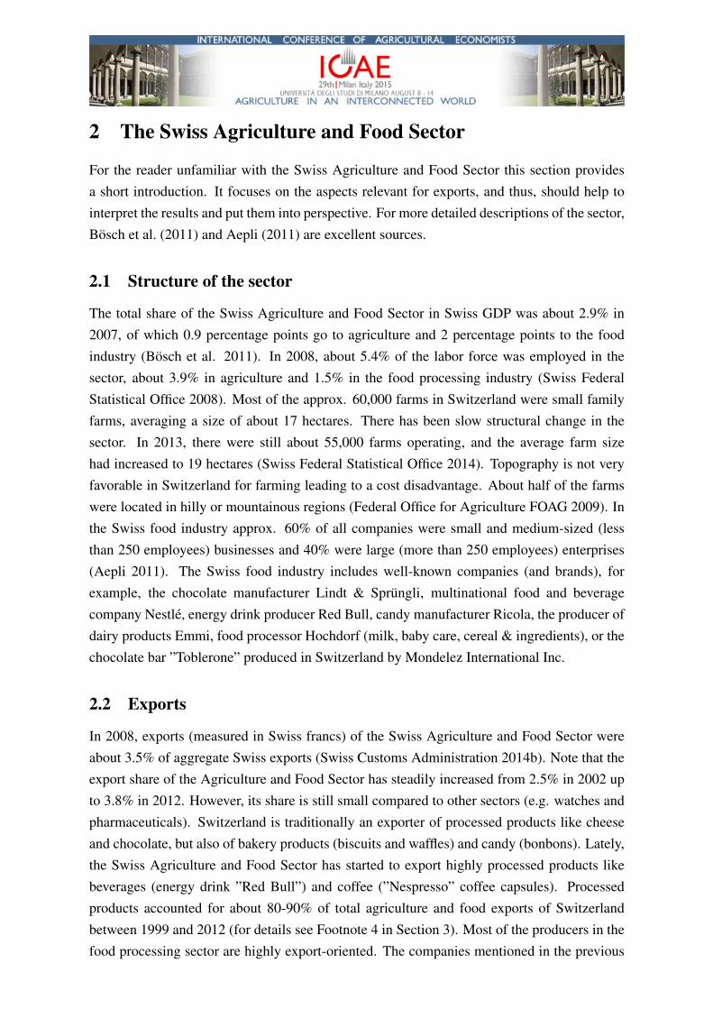
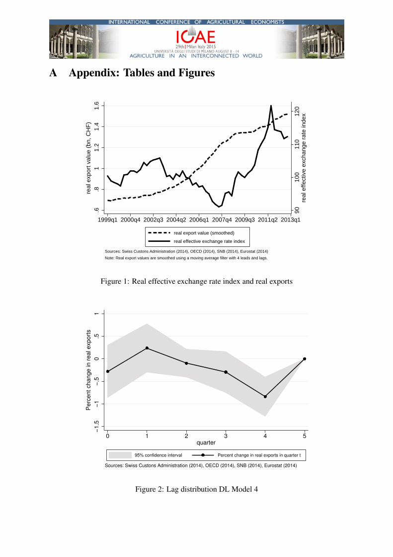
Figure 1 below shows the joint evolution of the real effective exchange rate index and realexports of the Swiss Agriculture and Food sector between 1999 and 2012. Between 1999and 2012, real agro-food exports increased from approx. CHF 0.7 billion per quarter to aboutCHF 1.5 billion per quarter. We see that the growth rate of real exports was higher in theyears right before the global financial crisis in 2008 than it has been since the aftermath of thefinancial crisis. At the same time, we observe that after 2002 the Swiss franc depreciatedabout 15 percent until the onset of the financial crisis in 2008, and appreciated stronglyafterwards until 2012 (approx. 20-30 percent). We note that during the depreciation of theSwiss franc between 2002 and 2008 exports increased at a higher rate than during the periodsof appreciation between 1999 and 2002, and more importantly, between 2008 and 2012. Thiscan be seen more clearly from Figure 4 in Appendix B, which depicts the percentage changesin real exports (smoothed) and in the real exchange real exchange rate index.

4 Examples of unprocessed products are HS categories ”01 Live Animals”, ”07 Edible Vegetables” or ”10Cereals”. Examples of processed products are found in HS categories ”04 Dairy, Eggs, Honey & EdibleProducts” (e.g. cheese), ”09 Coffee, Tea, Mate & Spices” (e.g. Nespresso coffee capsules), ”18 Cocoa & CocoaPreparations” (e.g. chocolate), ”19 Preparations of Cereals, Flour, Starch or Milk” (e.g. baby food, biscuits),”21 Miscellaneous Edible Preparations” (e.g. chewing gum, bonbons), ”22 Beverages, Spirits & Vinegar” (e.g.energy drink Red Bull), and ”24 Tobacco & Manufactured Tobacco Substitutes” (e.g. cigarettes). The latter 7HS categories of processed products mentioned above had a share of 80 to 90 percent in total agricultural andfood exports during the observation period (see Kohler 2014).

HERE: Figure 1

We approximate changes in foreign demand for Swiss agriculture and food productswith changes in aggregate GDP of Swiss trading partners (purchasing power parity adjusted,baseyear 2005), denoted by GDPt. In particular, we compute a weighted average of the 36countries’ GDPs using export shares as weights. The data is provided by OECD (2014). SeeAppendix B for details on the construction of the real effective exchange rate measure and thedemand variable.

Table 4 in Appendix B reports the results from augmented Dickey-Fuller andPhillips-Perron tests. The results show that the log transformed time series, log (Xt),log (GDPt) and log (RERt), are all integrated of order one, i.e. I(1). To make the timeseries weakly dependent (so that a law of large numbers and a central limit theorem apply),we transform each by first-differencing, i.e. xt ≡ ∆ log (Xt), gdpt ≡ ∆ log (GDPt),and rert ≡ ∆ log (RERt). Note that the first difference of a log transformed variableis approximately equal to the proportional percentage change in that variable. Hence, theobservations are quarter-to-quarter percentage changes (i.e. approximate quarterly growthrates). Appendix B also discusses the results from a Johanson test for co-integration. Theresults do not suggest that there exists a long-term relationship among the variables. Theappendix also provides summary statistics in Table 2.

3.2 Panel data

Since the panel dataset is based on the same data as the time series provided by the SwissCustoms Administration (2014b), we will keep its description brief.

The panel dataset contains the annual exports of 194 HS4 product categories (all HS4categories included in the HS2 classifications 01 to 24) to 36 countries (these correspond tothe same countries included in the time series data; see Table 3 in Appendix B) for the years2002 until 2012.5 The original dataset contains 194 × 36 × 11 = 76, 824 observations. Ascommon with disaggregated trade data, the data at the HS4 level include a large number ofzero observations for exports (approx. 68 percent). Since we log transform all variables inour analysis, we lose the zero observations. We construct a balanced panel, i.e. for exportsof a given product to a given country we observe a positive trade flow for every year between2002 and 2012, ending up with a dataset containing 12,716 observations. Again, we have dataon (bilateral) real exchange rates provided by the Swiss National Bank (2014) and Eurostat(2014), and on countries’ GDP by OECD (2014). Summary statistics for the balanced paneldata can be found in Table 5 in Appendix B.

5Examples for HS4 product categories include ”0406 Cheese and curd”, ”0901 Coffee, whether or not roastedor decaffeinated” (e.g. ”Nespresso” capsules), ”1806 Chocolate and other food preparations containing cocoa”,”1905 Bread, pastry, cakes and other bakers’ wares, whether or not containing cocoa”, ”2106 Food preparations,n.e.s.” (incl. bonbons), ”2202 Waters, incl. mineral waters and aerated waters, containing added sugar or othersweetening matter or flavored” (e.g. ”Red Bull”).

4 Time series analysis

This section introduces the time series models used to estimate the exchange rate effects,and discusses the results. From the discussion in Section 3.1, remember that the time seriesare integrated of order one, so that we take first-differences of the log transformed variables,and that we don’t find evidence for a co-integration relationship among the variables. Thus,we cannot apply (vector) error-correction models in our analysis. Instead, we will look atdistributed lag (DL) and autoregressive distributed lag (ADL) models.

4.1 Time series models

We start our analysis with a simple finite distributed lag (DL) model based on quarterly timeseries data. In particular, we want to test whether exchange rate movements (controlling fordemand changes) have a lagged effect on changes in exports. The reason is that we believelong-term contracts and consumption habits might matter in the context of exchange rateeffects. Thus, we estimate the following DL model by OLS

xt = α +K∑k=0

βkgdpt−k +J∑

j=0

γjrert−j + At + νt, (1)

where xt denotes the quarter-to-quarter percentage change in real exports, gdpt−k and rert−j

denote the kth and jth lag of the quarter-to-quarter percentage changes, in the weightedaggregate GDP of all trading-partners and the real effective exchange rate index, respectively.6

At includes quarterly dummies (capturing seasonal effects), a linear annual time trend(allowing for a trend in growth rates over the years) and a dummy variable indicatingthe introduction of the exchange rate peg against the Euro by the Swiss National Bank inSeptember 2011. We assume that the zero conditional mean assumption holds for the errorterm νt. DL models often have serial correlation in the error term, even if there is no underlyingmisspecification (see Wooldridge 2009). We know that this does not affect the consistency ofthe OLS estimator but makes inference based on OLS invalid. Thus, we compute Newey-Weststandard errors, which are robust to heteroskedasticity and autocorrelation in the error terms.7

DL models have the following drawbacks. In general, they impose strong, possibly incorrectrestrictions on the lagged response of the dependent variable to changes in an independent

6For OLS to be consistent we need that: (1) the time series are weakly dependent (so that a law of largenumbers and central limit theorem can be applied), (2) the zero conditional mean assumption holds, i.e. foreach t, E(νt|xt) = 0, where xt denotes the vector including all independent variables, and (3) there is noperfect collinearity. If assumptions (1)-(3) hold, OLS is consistent. However, note that OLS is biased if the strictexogeneity assumption, for each t, E(νt|X) = 0 fails. For more details see e.g. Wooldridge (2009) or Greene(2003).

7Even though OLS is inefficient in that case, it has some advantages to estimate the model by OLS andcorrect the standard errors for serial correlation, compared to other approaches like Feasible Generalized LeastSquares (FGLS). If the explanatory variables are not strictly exogenous, FGLS will not even be consistent (seeWooldridge 2009).

variable (Greene 2003). Keele and Kelly (2005) argue that with autocorrelated data one shouldbe hesitant to use OLS with corrected standard errors. Using Monte Carlo simulations theyshow that OLS can be severely biased in that case if the model is misspecified (i.e. the truedata generating process is dynamic). In particular, there is often multicollinearity, i.e. highautocorrelation of the independent variables. This makes it difficult to obtain precise estimatesof the individual coefficients. Nevertheless, it is often possible to obtain good estimates of thelong-run effect (Wooldridge 2009). In order to check how sensitive the results from the DLmodel are to model specification, we also estimate the following autoregressive distributed lag(ADL) model by OLS

xt = α +I∑

i=1

ρixt−i +K∑k=0

βkgdpt−k +J∑

j=0

γjrert−j + At + νt, (2)

where we added i lags of the dependent variable xt on the right-hand side. The rest of themodel specification is left unchanged compared to the DL model (1). We continue to assumethat the zero conditional mean assumption holds for the error term νt.8

We select the number of lags in both models according to Hayashi’s (2000)general-to-specific sequential t rule. Since we have quarterly data, we start at 4 lags of eachvariable, and sequentially exclude lags that are not statistically significant (at the 5% level).We further check for autocorrelation in the residuals after each elimination, using Durbin’salternative test and the Breusch-Godfrey LM test. Note that according to Hayashi (2000), thisrule has the disadvantage of possibly overfitting the model. Thus, as a check, we also look atthe Akaike information criterion (AIC) and the Bayesian information criterion (BIC).

4.2 Results and Discussion

This section discusses the DL model (1) and the ADL model (2) in turn, and compares theirresults. Our discussion of the results concentrates on the effect of changes in the real exchangerate of the Swiss franc on real exports. We further compare the results to the existing literaturefor Switzerland, and interpret them.

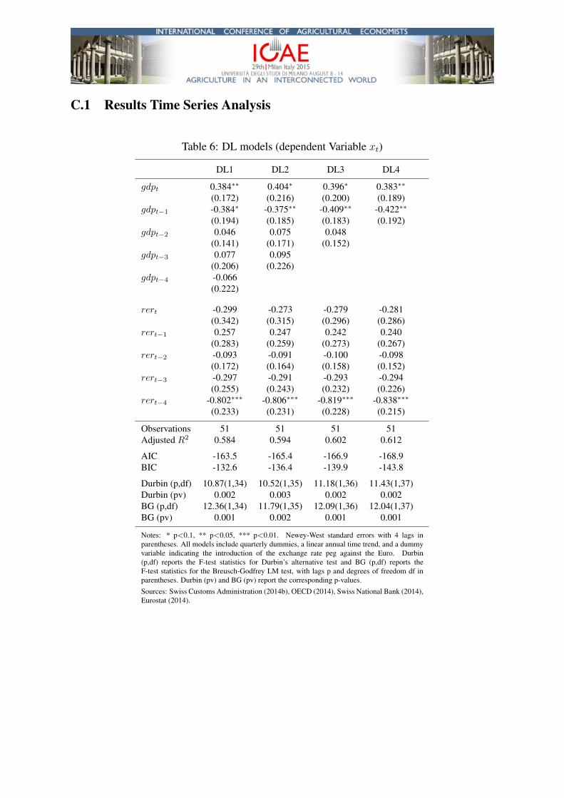
Table 6 in Appendix C reports the results for the DL model (1). Models DL1 to DL4show that the estimated exchange rate effects are fairly stable with respect to different model

8Note that models with lagged dependent variables cannot satisfy the strict exogeneity assumption. However,as long as the zero conditional mean assumption in Footnote 6 holds, OLS is consistent. In that case, the laggeddependent variables xt−i are said to be predetermined with respect to the error term νt. This has the followingimplications. Not only is xt−i realized before νt, but its realized value has no impact on the expectation of νt(Davidson and MacKinnon 2003). In our case, this requires that past quarterly growth rates of real exports areuncorrelated with unobserved factors νt affecting the contemporaneous growth rate of real exports. Greene(2003) states that the usual explanation for autocorrelation in the error term is serial correlation in omittedvariables. According to Wooldridge (2009), serial correlation in the error term of a dynamic model often indicatesthat the model has not been completely specified (i.e. not enough lags of the dependent variable have beenincluded). Hence, we test for (first-order) serial correlation in the error term using Durbin’s alternative test andthe Breusch-Godfrey LM test.

specifications. Hence, we focus our discussion on model DL4, which represents the mostparsimonious specification.

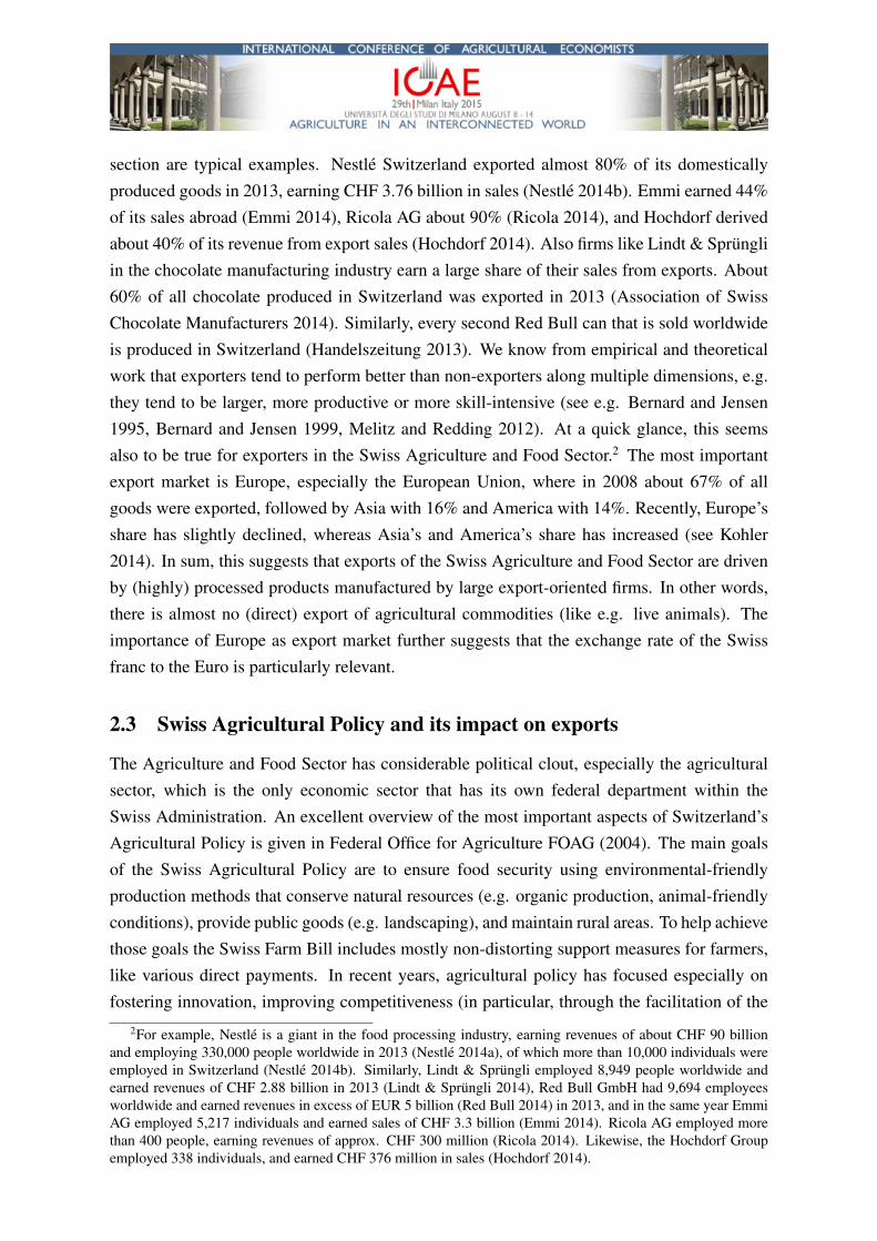
Figure 2 below shows the lag distribution of model DL4 (including a 95% confidenceinterval). We see that there is a lagged effect on real exports, 4 quarters after a change in thereal effective exchange rate. In particular, a temporary 1 percent appreciation of the Swissfranc today leads on average to a statistically significant decrease in real exports of about 0.8percent, 4 quarters from today, ceteris paribus. Note that a one percent appreciation in thecurrent quarter means that the price of the Swiss franc (relative to other currencies) raises byone percent in that quarter, e.g. the real exchange rate index increases from 100 to 101 andstays at that level. However, in the next quarter there is no further appreciation of the Swissfranc, e.g. the real exchange rate index stays at 101. Summing up over the coefficients γj givesa long-run exchange rate elasticity of approx.

∑j γj = −1.3, with a Newey-West standard

error of 0.324 (p-value 0.000). Here, the Swiss franc appreciates one percent four quarters ina row, e.g. the real exchange rate index raises from 100 to 104 in one year.

HERE: Figure 2

The results from the ADL model (2) are reported in Table 7 in Appendix C. Table 7 alsoincludes the F-test statistics for Durbin’s alternative test and for the Breusch-Godfrey (BG)LM test for first-order serial correlation (i.e. p=1) in the errors vt. Note that the tests neverreject the H0 of no (first-order) serial correlation in the errors at a level lower than 10 percent(except the BG test for model ADL4).9 Again, we see that the results are relatively stableacross the different model specifications ADL1 to ADL5. Thus, we focus our discussion onmodel ADL5, the most parsimonious specification. For model ADL5, Table 8 in AppendixC reports the F-test statistics also for higher-order serial correlation. A further issue in ADLmodels concerns stability. For the stochastic difference equation (2) to be stable we need that∑

i ρi < 1, which holds for all models ADL1 to ADL5.First, we look at temporary or short-run effects again. Due to the lagged dependent

variable, the effects of changes in the real exchange rate index on real exports have to becalculated.10 The lag distribution up to 12 lags including a 95% confidence interval for modelADL5 is depicted in Figure 3. We see that on average a 1 percent appreciation of the Swissfranc today only leads on average to a statistically significant decrease in real exports of about0.8 percent, 4 quarters or one year from today, ceteris paribus. All other lags are not significantat the 5% level. In other words, this one-time appreciation of the Swiss franc leads only to

9Note that we alternatively estimated the models with Newey-West standard errors robust to autocorrelationin the error terms (with 4 lags for quarterly data as suggested by Wooldridge 2009), and heteroskedasticity-robuststandard errors. In general, both Newey-West and heteroskedasticity-robust standard errors are slightly smallerthan conventional standard errors. Following the rule-of-thumb proposed by Angrist and Pischke (2008), wereport the largest standard errors to avoid misjudgments of precision.

10The impact elasticity (propensity) is given by γ0. The effect after one quarter is given by ργ0, after twoquarters by ρ2γ0 + ργ1 + γ2, after three quarters by ρ3γ0 + ρ2γ1 + ργ2 + γ3, and after h ≥ 4 quarters byρh−4

(ρ4γ0 + ρ3γ1 + ρ2γ2 + ργ3 + γ4

). The effects can be interpreted as elasticities.

a temporary (lagged) response in exports. Second, consider the permanent or long-run effectof exchange rate movements on exports. The permanent effect in model ADL5 is equal to∑

j γj/ (1−∑

i ρi) = −0.9 (standard error 0.382; p-value 0.021). This means that if theSwiss franc appreciates 1 percent every quarter, exports are on average 0.9 percent lower inevery quarter, ceteris paribus. Again, short-run elasticities are lower than long-run elasticities,which is intuitive. We would expect that the reaction to temporary shocks is lower than topermanent ones.

HERE: Figure 3

We note that the short- and long-run effects in the DL and ADL models are relativelysimilar. However, since the DL model imposes strong restrictions on the lagged response ofthe dependent variable to changes in the independent variables (i.e. misspecification), we havemore trust in the estimates based on the ADL models.

The estimated short- and long-run elasticities from the ADL models are broadly in linewith the literature on exchange rate effects for Switzerland. For example, SECO (2010)estimate a error correction model, and find that an appreciation of the Swiss franc by 1percent reduces aggregate Swiss exports by 0.4 percent in the short-run and by 1 percentin the long-run. Tressel and Arda (2011) also estimate an error correction model for aggregateSwiss exports. They also find a long-run elasticity of exports with respect to exchange ratechanges of -0.9. Lamla and Lassmann (2011) estimate a ADL model for 6 export markets(Germany, France, Italy, UK, US, Japan) and 12 sectors, separately. For the agriculture andfood sector they don’t find any significant effects of exchange rate movements on exports toany of the 6 export markets.

Even though, temporary and permanent effects are statistically significant they areeconomically relatively small. The results further suggest that temporary responses ofexchange rate movements are most likely lagged. This could be because of long-termcontracts, persistent consumption habits but also because firms, especially large exporters likeNestle, Lindt & Sprungli and Red Bull, might hedge their foreign exchange rate risk in thecurrency market. Hedging could also explain why the effects on average are economicallyrelatively small. Other reasons might be that Swiss producers can successfully differentiatetheir products on foreign markets, e.g. with the help of umbrella brands like ”Swissness” orfirm-specific brands like ”Nespresso”. They mostly produce high-quality specialties for nichemarkets, e.g. cheese specialties like Gruyere cheese or Swiss chocolate, characterized by lowcompetition and a relatively high degree of market power. Summa summarum, this suggeststhat the focus of the Swiss Agricultural Policy on a quality strategy might help to mitigate theeffects of exchange rate changes, at least for domestic producers of raw products. However,the effects of an appreciation of the Swiss franc might also be dampened if imported inputgoods become cheaper. The results could as well be interpreted in the sense, that on average

producers in the Swiss Agriculture and Food Sector face relatively inelastic foreign demand(i.e. the price elasticity of demand is low).

5 Panel data analysis

To complement the time series analysis above, we estimate dynamic panel data models basedon the panel data described in Section 3.2. This allows us to further check the robustness ofthe results from the time series analysis. The advantage is that the panel data allow us to usethe information contained in the cross-section, which should lead to more efficient and lessbiased estimates.

5.1 Dynamic panel data models

Economic reasoning suggests that lagged effects might be important in the context of exchangerate effects. This is also implied by the time series analysis in the previous section. Hence,consider the following dynamic panel data model

log (Xijt) = α + ρXij,t−1 + β log (GDPit) + γ log (RERit) + Ai + Aj + At + νijt

where i indexes countries, j products, and t time.11 The terms Ai, Aj , and At denotetrading-partner (country), product and time fixed-effects, respectively. The (idiosyncratic)error term νijt is assumed to be independent and identically distributed (i.i.d.).

We follow the usual procedure in the literature (see e.g. Angrist and Pischke 2008,Roodman 2009), and transform the model above by taking first-differences

∆ log (Xijt) = ρ∆ log (Xij,t−1) + β∆ log (GDPit) + γ∆ log (RERit) + ∆At + ∆νijt, (3)

killing the fixed-effects Ai and Aj . Note that even though the fixed-effects are gone now,the lagged dependent variable ∆ log (Xij,t−1) is still correlated with the errors ∆νijt, sincethe latter contains νijt and the former log (Xij,t−1); the classic reference is Nickell (1981).However, with the fixed-effects eliminated, equation (3) can be estimated using instrumentalvariables (IV). Instruments for ∆ log (Xij,t−1) can be constructed from second and higherlags of log (X), either in levels or differences. If νijt is i.i.d., those lags will be correlatedwith ∆Xij,t−1 but uncorrelated with ∆εijt. We will test whether this assumption holds byreporting the value of the Arellano-Bond AR(2) test on the residuals in first differences (i.e. todetect AR(1) in the underlying levels variables). Furthermore, we test whether the instrumentspass the Hansen J test for over-identification (as suggested by Roodman 2009, we don’t takecomfort in a p-value below 0.1 and are suspicious of p-values above 0.25).

11Similar to ADL model (2) in Section 4.1, the impact elasticity (propensity) is given by γ, the lagged effectafter h ≥ 1 years is given by ρhγ. The long-run elasticity is given by γ/(1− ρ).

There are several dynamic panel data estimators available (see e.g. Baum 2013). As astarting point, equation (3) is often estimated using two-stage least-squares (2SLS), followingAnderson and Hsiao (1982). They propose the use of either second- or higher-order lags ofthe lagged dependent variable (either in levels or first differences) as instruments. Arellano(1989) argues that the estimator using instruments in levels has much smaller variances, andis therefore preferred. While the Anderson-Hsiao (A-H) estimator is consistent, Arellano andBond (1991) argue that it is not efficient since it fails to take all the potential orthogonalityconditions into account. Hence, we also estimate model (3) using the Arellano-Bond (A-B)difference GMM one-step and two-step estimator (see Arellano and Bond 1991). Accordingto Roodman (2009) the A-B two-step GMM estimator with Windmeijer (2005) correctedstandard errors seems slightly superior to the A-B one-step GMM estimator with cluster-robuststandard errors (lower bias and standard errors). Hence, our discussion of the results in thefollowing section focuses on the results from the A-B two-step difference GMM estimatorwith Windmeijer-corrected standard errors.

5.2 Results and Discussion

Table 1 below reports the results from the A-B two-step GMM estimator.12 We report theresults from model A-B M1 using all instruments, model A-B M2 using the collapsed set ofinstruments (see Roodman 2009), and models A-B M1 to A-B M8, which are the only modelswith valid instruments. First, note that models A-B M1 and A-B M2 are not valid sincethey fail both the Arellano-Bond AR(2) test, and the Hansen J test. Second, note that theestimated short-run exchange rate elasticities (given by the coefficients on ∆ log (RERit)),and long-run exchange rate elasticities (LRE) are all very similar across the valid modelsA-B M1 to A-B M8. However, looking at AR(2) and Hansen J test statistics, we prefermodel A-B M7 (using lags 6 to 9 as instruments), since we can be most confident thatthe instruments used in this model are valid. In particular, the Arellano-Bond AR(2) testsuggests that there is no second-order serial correlation in the error term, and the p-value ofthe Hansen J test for over-identification lies between 0.1 and 0.25 (remember the discussionin the previous section). However, note that the results from the A-H 2SLS estimators andthe A-B one-step difference GMM estimators are very similar, see Table 9 and Table 10,respectively, in Appendix C.2.

Nevertheless, in the following discussion we focus on model A-B M7. We see that theestimated short- and long-run exchange rate elasticities are given by approx. -0.5, and -0.8,

12In principle, one might argue that GDP and the real exchange rate index too could be endogenous in model(3). In other words, there might be unobserved shocks that affect both changes in the exchange rate as well aschanges in agro-food exports. We don’t think this is a problem here. However, the A-B framework offers anatural set of instruments (in the form of lagged values of GDP and the real exchange rate index) to address thisissue. Hence, we also look at A-B difference GMM estimators treating GDP and the real exchange rate index asendogenous. We find statistically significant short- and long-run exchange rate elasticities that are about twice aslarge compared to the ones in Table 1.

respectively. This means that a 1 percent appreciation of the Swiss franc leads in the short- andlong-run on average to a reduction of 0.5 percent and 0.8 percent in real exports, respectively.As in the time series analysis, we see that the long-run elasticities are higher than the short-runelasticities. Again, this is intuitive since the reactions to temporary shocks are expected to besmaller than to permanent ones.

Most studies estimate exchange rate effects based on time series, neglecting the paneldimension. Thus, studies which use panel data to estimate exchange rate elasticities arerelatively uncommon. A notable exception is Auer and Saure (2011), who estimate dynamicpanel data models for 25 product categories and 27 countries. They find that a 1 percentappreciation of the Swiss franc has a negative effect on exports of about 0.7 percent in thelong-run, which is very similar to our own estimate. Another exception is Gaillard (2013),who estimates static panel data models.13 She finds long-run exchange rate elasticities in therange of -0.5 to -0.8.

Comparing the short- and long-run elasticities based on panel data with the ones basedon time series, we see that the elasticities based on time series (-0.8 and -0.9, respectively)are slightly higher than the ones based on panel data (-0.6 and -0.8, respectively). However,any small sample bias of the estimates based on (autoregressive) time series models seems tobe small. Thus, our basic interpretation of the results in Section 4.2 does not change. Sincethe panel data analysis suggests that the effects are economically even smaller, we have moreconfidence in our interpretation, that on average producers are able to successfully evade pricecompetition. Here, one should note that this is the average reaction of exports to exchange ratechanges. In other words, the exports of some business sectors within the Swiss Agricultureand Food Sector might react less or more to exchange rate changes. Furthermore, this doesnot necessarily imply that overall firm performance isn’t affected at all if the Swiss francappreciates or depreciates (see e.g. Swiss National Bank 2011). For example, profit marginsmight fall, investments could be put on hold, or there may be negative employment effects(e.g. lay-offs, cut in working hours) if the Swiss franc appreciates. Hence, it would be foolishto conclude that all is well for every producer in the Swiss Agriculture and Food Sector if theSwiss franc appreciates strongly. However, our analysis suggests that not all is lost - at leaston average the effects of exchange rate changes on the export performance of producers arerelatively small.

HERE: Table 113We also estimate the following static panel data model

∆ log (Xijt) = α+ β∆ log (GDPit) + γ∆ log (RERit) +Ai +Aj +At + εijt.

The static panel data model has the advantage that it does not rely on instrumental variables. The downside is thatif the underlying data generating process is dynamic, the model is misspecified. However, the estimated short-runelasticity is -0.6 (standard error 0.186; p-value 0.001), and is similar to the short-run elasticties estimated fromdynamic panel data models.

6 Conclusion

After the global financial crisis in 2008 the Swiss franc has appreciated strongly against thecurrencies of Switzerland’s most important trading partners. This has raised the old questionof how sensitive exports react to exchange rate changes. We investigate this question for theexports of the Swiss Agriculture and Food Sector. Focusing on the Swiss Agriculture andFood Sector has the advantage that the sector is economically small, so that we don’t have toworry about reverse causality of exchange rate fluctuations.

We use time series and panel data models to estimate short- and long-run exchange rateelasticities. This allows us to assess how sensitive the results are with respect to modelspecification, estimation methods and data structure. We find that the estimated elasticitiesare remarkably similar across all models and estimation methods. However, in general,the estimates based on panel data are slightly lower than the ones on time series. In theshort-run, we find that a (temporary) appreciation of one percent of the Swiss franc implieson average a (lagged) decrease in real exports of agriculture and food exports between 0.6and 0.8 percent, one year after the appreciation. In the long-run, we find that on average aone percent appreciation of the Swiss franc leads to a (permanent) decrease in real exportsin the range of 0.8 to 0.9 percent. These estimates are similar to the findings of studieson aggregate Swiss exports. The estimated exchange rate effects seem economically small.It seems that on average, producers in the Swiss Agriculture and Food Sector are able toevade price competition by successfully differentiating their products, producing high-qualityproducts for niche markets. This further suggests that the emphasis on product quality in theSwiss Agricultural Policy is an adequate strategy for Swiss producers to successfully competeon foreign markets. These might be a valuable lesson for policy makers in other industrializedcountries with similar agriculture and food sectors (e.g. Norway, Japan) that could be learnedfrom Switzerland. However, we think that these lessons can also be generalized to othersectors to some extent. Most other sectors of the Swiss economy also pursue a qualitystrategy (e.g. mechanical watches, precision instruments and mechanical appliances, electricmachinery, pharmaceuticals). As previously discussed, studies looking at the aggregate Swisseconomy find exchange rate elasticities in the same range as we find for the agriculture andfood sector.

Future research could focus on the case study of a particular product market, e.g. cheese,chocolate or biscuits, that might help us to better understand the mechanisms/channels throughwhich the exchange rate operates. Further research could also look at the effects of exchangerate volatility on exports of agriculture and food products. This might yield some insight intohow uncertainty of price changes, proxied by exchange rate volatility, affects exports in theagriculture and food sector. Furthermore, it would be interesting to study how import pricechanges, due to exchange rate changes, are passed through to domestic producer and consumerprices.

ReferencesAepli, M. (2011). Volkswirtschaftliche Bedeutung und Wettbewerbsfahigkeit der Schweizer

Nahrungsmittelindustrie. Masterarbeit Institut fur Umweltentscheidungen ETH Zurich.

Anderson, T. and Hsiao, C. (1982). Formulation and estimation of dynamic models usingpanel data. Journal of Econometrics, 18(1):47–82.

Angrist, J. D. and Pischke, J.-S. (2008). Mostly Harmless Econometrics: An Empiricist’sCompanion. Princeton University Press, Princeton, NJ.

Arellano, M. (1989). A note on the Anderson-Hsiao estimator for panel data. EconomicsLetters, 31(4):337–341.

Arellano, M. and Bond, S. (1991). Some Tests of Specification for Panel Data: Monte CarloEvidence and an Application to Employment Equations. The Review of Economic Studies,2(2):277–297.

Association of Swiss Chocolate Manufacturers (2014). Facts & Figures.http://www.chocosuisse.ch/chocosuisse/en/documentation.html.

Auer, R. and Saure, P. (2011). CHF Strength and Swiss Export Performance - Evidence andOutlook From a Disaggregate Analysis. Working Paper 11.03, Swiss National Bank, StudyCenter Gerzensee.

Baum, C. F. (2013). Dynamic Panel Data estimators. Lecture Notes Boston College.

Bernard, A. B. and Jensen, J. B. (1995). Exporters, Jobs, and Wages in US Manufacturing:1976-87. Brookings Papers on Economic Activity: Microeconomics, pages 67–112.

Bernard, A. B. and Jensen, J. B. (1999). Exceptional Exporter Performance: Cause, Effect, orBoth? Journal of International Economics, 47(1):1–25.

Bosch, I., Weber, M., Aepli, M., and Werner, M. (2011). Folgen unterschiedlicherOffnungsszenarien fur die Schweizer Nahrungsmittelindustrie. Untersuchung zuhanden vonEconomiesuisse, Migros, Nestle (Schweiz) und IGAS.

Chit, M. M., Rizov, M., and Willenbockel, D. (2010). Exchange Rate Volatility and Exports:New Empirical Evidence from the Emerging East Asian Economies. The World Economy,33(2):239–263.

Davidson, R. and MacKinnon, J. G. (2003). Econometric Theory and Methods. OxfordUniversity Press, New York, NY.

Dudda, E. (2013). Schoggigesetz versusst auch Margen. Schweizer Bauer.

Emmi (2014). Annual Report 2013. http://group.emmi.com/en/media-ir/publications.html.

Eurostat (2014). Eurostat database.

Federal Office for Agriculture FOAG (2004). Swiss Agricultural Policy. Publication BLW.

Federal Office for Agriculture FOAG (2009). Agrarbericht 2009 des Bundesamtes furLandwirtschaft. Agrarbericht.

Federal Office for Agriculture FOAG (2013). Verordnung uber die Forderung von Qualitatund Nachhaltigkeit in der Land- und Ernahrungswirtschaft (QuNaV). Das Neueste zurAgrarpolitik 2014-2017.

Federal Office for Agriculture FOAG (2014). Freihandelsabkommen.

http://www.blw.admin.ch/themen/00009/01208/index.html?lang=de.

Fluri, R. and Muller, R. (2001). Die Revision der nominellen und realen exportgewichtetenWechselkursindizes des Schweizer Frankens. Schweizerische Nationalbank Quartalsheft,19(3).

Furer, O. (2013). Der Einfluss des Wechselkurses auf die Exporte der Schweiz - Eineempirische Analyse. Masterarbeit Universitat St. Gallen.

Gaillard, S. (2013). The effects of real exchange rates on the Swiss balance of trade. Master’sThesis Department of Economics at the University of Zurich.

Greene, W. H. (2003). Econometric Analysis. Prentice Hall, Upper Saddle River, NJ.

Grisse, C. and Nitschka, T. (2013). On financial risk and the safe haven characteristics ofSwiss franc exchange rates. Swiss National Bank Working Papers.

Handelszeitung (2013). Jede zweite Red-Bull-Dose kommt aus der Schweiz. Handelszeitung.

Hayashi, F. (2000). Econometrics. Princeton University Press, Princeton, NJ.

Hochdorf (2014). 118th Annual Report 2013. http://www.hochdorf.com/en/investors/.

Husted, S. and Melvin, M. (2009). International Economics. Prentice Hall, Upper SaddleRiver, NJ, 8 edition.

Keele, L. and Kelly, N. J. (2005). Dynamic Models for Dynamic Theories: The Ins and Outsof Lagged Dependent Variables. Working Paper.

Kim, M., Cho, G. D., and Koo, W. W. (2004). Does the Exchange Rate Matter to AgriculturalTrade between Canada and the U.S.? Canadian Journal of Agricultural Economics,52(1):127–145.

Kohler, A. (2014). Determinanten der Schweizer Agrarexporte - Eine Anwendung desokonomischen Gravitationsmodells. Journal of Socio-Economics in Agriculture.

Kristinek, J. J. and Anderson, D. P. (2002). Exchange Rates and Agriculture: A LiteratureReview. Working Paper Agricultural and Food Policy Center Texas A&M University.

Lamla, M. and Lassmann, A. (2011). Der Einfluss der Wechselkursentwicklung auf dieSchweizerischen Warenexporte: Eine Disaggregierte Analyse. KOF Analysen.

Lindt & Sprungli (2014). Annual Report 2013. http://www.lindt.ch/swf/ger/investors/.

Melitz, M. J. and Redding, S. J. (2012). Heterogeneous Firms and Trade. NBER WorkingPaper 18652.

Nestle (2014a). Annual Report 2013. http://www.nestle.com/aboutus/annual-report.

Nestle (2014b). Facts & Figures. http://www.nestle.ch/de/nestleschweiz/factsandfigures.

Nickell, S. (1981). Biases in Dynamic Models with Fixed Effects. Econometrica,49(6):1417–1426.

OECD (2014). OECD.Stat.

Red Bull (2014). The Company Behind the Can. http://energydrink-us.redbull.com/company.

Ricola (2014). Wachstum Trotz Widrigem Wahrungsumfeld.http://www.ricola.com/de-ch/Meta/Medien/Medienmitteilungen.

Roodman, D. (2009). How to do xtabond2: An introduction to difference and system GMM

in Stata. The Stata Journal, 9(1):86–136.

Santos, C. H. D., Shaikh, A., and Zezza, G. (2003). Measures of the Real GDP of U.S. TradingPartners: Methodology and Results. Working Paper 387.

Schochli, H. (2014). Nachspiel zur Swissness-Debatte. Neue Zurcher Zeitung.

SECO (2010). Aussenhandelsentwicklung der Schweiz im Jahr 2009. KonjunkturtendenzenFruhjahr 2010.

Swiss Customs Administration (2014a). Ausfuhrbeitrage fur Erzeugnisse ausLandwirtschaftsprodukten. http://www.ezv.admin.ch/index.html?lang=en.

Swiss Customs Administration (2014b). Foreign trade statistics Swiss-Impex.

Swiss Federal Statistical Office (2008). Vom Feld bis auf den Teller - Die Lebensmittelkettein der Schweiz. BFS Aktuell.

Swiss Federal Statistical Office (2014). Landwirtschaft.http://www.bfs.admin.ch/bfs/portal/de/index/themen/07/03.html.

Swiss National Bank (2011). Exchange rate survey: Effects of Swiss franc appreciation andcompany reactions. Quarterly Bulletin.

Swiss National Bank (2014). G2a Wechselkursindizes - Lander. Statistisches Monatsheft.

Tressel, T. and Arda, A. (2011). Switzerland: Selected Issues Paper. IMF Country Report No.11/116.

Vellianitis-Fidas, A. (1976). The Impact of Devaluation on U.S. Agricultural Exports.Agricultural Economics Research, 28(3):107–116.

Windmeijer, F. (2005). A finite sample correction for the variance of linear efficient two-stepGMM estimators. Journal of Econometrics, 126(1):25–52.

Wooldridge, J. M. (2009). Introductory Econometrics: A Modern Approach. CengageLearning EMEA, 4 edition.

A Appendix: Tables and Figures

9010

011

012

0re

al e

ffect

ive

exch

ange

rat

e in

dex

.6.8

11.

21.

41.

6re

al e

xpor

t val

ue (

bn, C

HF

)

1999q1 2000q4 2002q3 2004q2 2006q1 2007q4 2009q3 2011q2 2013q1

real export value (smoothed)

real effective exchange rate index

Sources: Swiss Custons Administration (2014), OECD (2014), SNB (2014), Eurostat (2014)

Note: Real export values are smoothed using a moving average filter with 4 leads and lags.

Figure 1: Real effective exchange rate index and real exports

−1.5

−1

−.5

0.5

1

Perc

ent change in r

eal export

s

0 1 2 3 4 5quarter

95% confidence interval Percent change in real exports in quarter t

Sources: Swiss Custons Administration (2014), OECD (2014), SNB (2014), Eurostat (2014)

Figure 2: Lag distribution DL Model 4

−1.

5−

1−

.50

.51

Per

cent

cha

nge

in r

eal e

xpor

ts

0 1 2 3 4 5 6 7 8 9 10 11 12quarter

95% confidence interval Percent change in real exports in quarter t

Sources: Swiss Custons Administration (2014), OECD (2014), SNB (2014), Eurostat (2014)

Figure 3: Lag distribution ARDL Model 5

Table 1: Arellano-Bond two-step difference GMM estimators (dep Var ∆ log (Xijt))

A-B M1 A-B M2 A-B M3 A-B M4 A-B M5 A-B M6 A-B M7 A-B M8all collapsed lag5 lag6to7 lag6to8 lag7to8 lag6to9 lag7to9

∆ log (Xij,t−1) 0.361∗∗∗ 0.350∗∗∗ 0.219 0.483 0.322 0.097 0.319 0.170(0.043) (0.043) (0.307) (0.318) (0.289) (0.419) (0.278) (0.322)

∆ log (GDPit) 1.019∗∗ 1.070∗∗ 1.097∗ 0.741 0.975∗ 1.260∗ 0.963∗ 1.122∗

(0.462) (0.465) (0.624) (0.631) (0.581) (0.762) (0.578) (0.666)

∆ log (RERit) -0.654∗∗∗ -0.546∗∗∗ -0.537∗∗ -0.476∗∗ -0.534∗∗ -0.570∗∗∗ -0.543∗∗∗ -0.575∗∗∗

(0.197) (0.207) (0.224) (0.225) (0.210) (0.209) (0.206) (0.206)

LRE -1.023∗∗∗ -0.840∗∗∗ -0.687∗∗ -0.920 -0.788∗∗ -0.631∗∗ -0.797∗∗ -0.693∗∗

(0.314) (0.319) (0.321) (0.583) (0.379) (0.298) (0.380) (0.318)

Observations 10404 10404 10404 10404 10404 10404 10404 10404No Instruments 56 20 16 18 20 16 21 17AR(2) test (pv) 0.000 0.000 0.362 0.091 0.187 0.722 0.176 0.472Hansen J (df) 44 8 4 6 8 4 9 5Hansen J (pv) 0.000 0.029 0.101 0.185 0.135 0.234 0.176 0.285

Notes: * p<0.1, ** p<0.05, *** p<0.01. Cluster-robust standard errors in parentheses (Windmeijer 2005 finite-sample correction).Arellano-Bond two-step difference GMM estimator, assuming that GDP and RER are strictly exogenous. All models include yeardummies. LRE denotes the long-run real exchange rate elasticity. AR(2) test reports the p-value for the Arellano-Bond test for AR(2)in first differences. Hansen J (df) and (pv) report the degrees of freedom and the p-value for the Hansen J test of overidentifyingrestrictions, respectively.Sources: Swiss Customs Administration (2014b), OECD (2014), Swiss National Bank (2014), Eurostat (2014).

B Appendix: Data

B.1 Time Series Data

Table 2 below reports the summary statistics for the time series data over the whole sampleperiod 1999-2012 for real exports Xt, the demand measure GDPt, and the real effectiveexchange rate index RERt, where variables are in (natural) logarithms. Our sample consistsof 56 observations, i.e. we observe all variables in every quarter t between 1999 and 2012. InFigure 4, quarterly percentage changes in real exports (smoothed) and in the real exchange rateindex are shown over time. Table 3 below lists all countries in the sample, and their officialcurrencies.

Table 2: Summary statistics time series

min mean max sd T

log (Xt) -0.451 0.004 0.518 0.291 56log (GDPt) 0.625 0.902 1.191 0.137 56log (RERt) 4.510 4.623 4.802 0.062 56Sources: Swiss Customs Administration (2014b), OECD (2014), SwissNational Bank (2014), Eurostat (2014).

−.0

50

.05

perc

enta

ge c

hange

1999q2 2000q4 2002q2 2003q4 2005q2 2006q4 2008q2 2009q4 2011q2 2012q4

growth rate export value (smoothed)

change in exchange rate index

Sources: Swiss Custons Administration (2014), OECD (2014), SNB (2014), Eurostat (2014)

Note: Quarterly percentage changes in real export value and real effective exchange rate index.

Figure 4: Quarterly percentage changes in real effective exchange rate index and real exports

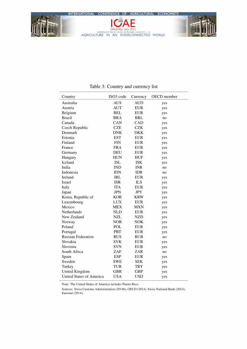
Table 3: Country and currency list

Country ISO3 code Currency OECD member

Australia AUS AUD yesAustria AUT EUR yesBelgium BEL EUR yesBrazil BRA BRL noCanada CAN CAD yesCzech Republic CZE CZK yesDenmark DNK DKK yesEstonia EST EUR yesFinland FIN EUR yesFrance FRA EUR yesGermany DEU EUR yesHungary HUN HUF yesIceland ISL ISK yesIndia IND INR noIndonesia IDN IDR noIreland IRL EUR yesIsrael ISR ILS yesItaly ITA EUR yesJapan JPN JPY yesKorea, Republic of KOR KRW yesLuxembourg LUX EUR yesMexico MEX MXN yesNetherlands NLD EUR yesNew Zealand NZL NZD yesNorway NOR NOK yesPoland POL EUR yesPortugal PRT EUR yesRussian Federation RUS RUB noSlovakia SVK EUR yesSlovenia SVN EUR yesSouth Africa ZAF ZAR noSpain ESP EUR yesSweden SWE SEK yesTurkey TUR TRY yesUnited Kingdom GBR GBP yesUnited States of America USA USD yes

Note: The United States of America includes Puerto Rico.Sources: Swiss Customs Administration (2014b), OECD (2014), Swiss National Bank (2014),Eurostat (2014).

Real exports Xt are measured in billion Swiss francs, and are obtained by deflatingnominal exports using the (mean) export price index for agriculture and food products (i.e.based on HS 01-24) provided by the Swiss Customs Administration (2014b). Deflatingnominal exports eliminates influences from price changes. Export values are based on invoicedprices in Swiss francs free on board (f.o.b.) at the Swiss border, i.e. prices are exemptinternational shipping costs.

The definition of the demand measure GDPt in period t follows Santos et al. (2003), andis given by

GDPt = exp

(1∑n

i=1wit

n∑i=1

wit lnGDPit

),

where the weight wit ≡ Xit/∑n

i=1Xit denotes the share of country i in total Swiss exports,and n denotes the total number of countries in the sample. Note that the demand measure isbased on GDP data measured in trillion Swiss francs (PPP adjusted, 2005).

The construction of the real effective exchange rate index RER in period t is based onFluri and Muller (2001), and given by

RERt =n∏

i=1

(Rit)12

(wiB+

witRit∑ni=1

witRit

),

where Rit =eiBCPIiBCPICH,t

eitCPIitCPICH,Bdenotes the real exchange rate index of country i in period

t, e denotes the nominal exchange rate (defined as units of Swiss francs per unit of foreigncurrency), andCPI is the consumer price index. The weightwit is defined as above. SubscriptB denotes the base period, and subscript CH stands for Switzerland.

Figure 5 below shows the joint evolution of the demand measure GDPt and real exportsXt of the Swiss Agriculture and Food Sector between 1999 and 2012. We see that demandand exports grow almost pari passu during the observation period.

As discussed above for OLS to be valid, we need the time series to be weakly dependent,i.e. integrated of order zero I(0). Table 4 reports the results of augmented Dickey-Fuller (ADF)and Phillips-Perron (PP) tests. Whereas the ADF test never rejects the null hypothesis of a unitroot in the level of all log transformed variables, the PP test doesn’t reject only in the case ofRER. Nevertheless, we take the first difference ∆ of all log transformed variables. Here, theADF and the PP tests agree (except for real exports xt), and we reject the null hypothesis thatthe log transformed variables in first differences contain a unit root. In other words, the logtransformed variables seem to be integrated of order one I(1).

We also test whether variables are co-integrated. To this end, we run a Johansen test (with2 lags). We cannot reject the null hypothesis of no co-integration among the variables at the5% level (i.e. the trace statistic of 20.38 at rank zero falls short of the 5% critical value of29.68). Hence, we don’t find evidence for the existence of a co-integration relationship.

22.

22.

42.

62.

83

GD

P (

smoo

thed

)

.6.8

11.

21.

41.

6re

al e

xpor

t val

ue (

bn, C

HF

)

1999q1 2000q4 2002q3 2004q2 2006q1 2007q4 2009q3 2011q2 2013q1

real export value (smoothed)

GDP (smoothed)

Sources: Swiss Custons Administration (2014), OECD (2014), SNB (2014), Eurostat (2014)

Note: Real export values and GDP are smoothed using a moving average filter with 4 leads and lags.

Figure 5: GDP and real exports

Table 4: Unit root testsADF test PP test

test stats p-value test stats p-value

log (Xt) -1.88 0.66 -3.95 0.01xt -2.91 0.16 -11.65 0.00

log (RERt) -1.16 0.92 -1.18 0.91rert -6.93 0.00 -6.93 0.00

log (GDPt) -2.30 0.43 -4.70 0.00gdpt -4.39 0.00 -10.46 0.00

Notes: All variables in (natural) logarithm. The table reports test statistics and the MacKinnonapproximate p-values. Augmented Dickey-Fuller (ADF) and Phillips-Perron (PP) tests (H0:unit root) both include a time trend. The number of lags has been chosen according toSchwarz’s Bayesian information criterion (SBIC).

Sources: Swiss Customs Administration (2014b), OECD (2014), Swiss National Bank (2014),Eurostat (2014).

B.2 Panel Data

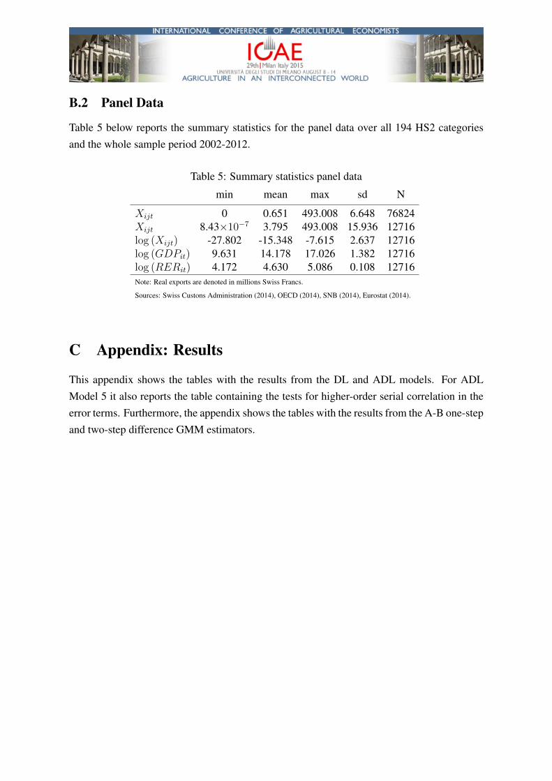
Table 5 below reports the summary statistics for the panel data over all 194 HS2 categoriesand the whole sample period 2002-2012.

Table 5: Summary statistics panel data

min mean max sd N

Xijt 0 0.651 493.008 6.648 76824Xijt 8.43×10−7 3.795 493.008 15.936 12716log (Xijt) -27.802 -15.348 -7.615 2.637 12716log (GDPit) 9.631 14.178 17.026 1.382 12716log (RERit) 4.172 4.630 5.086 0.108 12716Note: Real exports are denoted in millions Swiss Francs.

Sources: Swiss Custons Administration (2014), OECD (2014), SNB (2014), Eurostat (2014).

C Appendix: Results

This appendix shows the tables with the results from the DL and ADL models. For ADLModel 5 it also reports the table containing the tests for higher-order serial correlation in theerror terms. Furthermore, the appendix shows the tables with the results from the A-B one-stepand two-step difference GMM estimators.

C.1 Results Time Series Analysis

Table 6: DL models (dependent Variable xt)

DL1 DL2 DL3 DL4

gdpt 0.384∗∗ 0.404∗ 0.396∗ 0.383∗∗

(0.172) (0.216) (0.200) (0.189)gdpt−1 -0.384∗ -0.375∗∗ -0.409∗∗ -0.422∗∗

(0.194) (0.185) (0.183) (0.192)gdpt−2 0.046 0.075 0.048

(0.141) (0.171) (0.152)gdpt−3 0.077 0.095

(0.206) (0.226)gdpt−4 -0.066

(0.222)

rert -0.299 -0.273 -0.279 -0.281(0.342) (0.315) (0.296) (0.286)

rert−1 0.257 0.247 0.242 0.240(0.283) (0.259) (0.273) (0.267)

rert−2 -0.093 -0.091 -0.100 -0.098(0.172) (0.164) (0.158) (0.152)

rert−3 -0.297 -0.291 -0.293 -0.294(0.255) (0.243) (0.232) (0.226)

rert−4 -0.802∗∗∗ -0.806∗∗∗ -0.819∗∗∗ -0.838∗∗∗

(0.233) (0.231) (0.228) (0.215)

Observations 51 51 51 51Adjusted R2 0.584 0.594 0.602 0.612

AIC -163.5 -165.4 -166.9 -168.9BIC -132.6 -136.4 -139.9 -143.8

Durbin (p,df) 10.87(1,34) 10.52(1,35) 11.18(1,36) 11.43(1,37)Durbin (pv) 0.002 0.003 0.002 0.002BG (p,df) 12.36(1,34) 11.79(1,35) 12.09(1,36) 12.04(1,37)BG (pv) 0.001 0.002 0.001 0.001

Notes: * p<0.1, ** p<0.05, *** p<0.01. Newey-West standard errors with 4 lags inparentheses. All models include quarterly dummies, a linear annual time trend, and a dummyvariable indicating the introduction of the exchange rate peg against the Euro. Durbin(p,df) reports the F-test statistics for Durbin’s alternative test and BG (p,df) reports theF-test statistics for the Breusch-Godfrey LM test, with lags p and degrees of freedom df inparentheses. Durbin (pv) and BG (pv) report the corresponding p-values.Sources: Swiss Customs Administration (2014b), OECD (2014), Swiss National Bank (2014),Eurostat (2014).

Table 7: ADL models (dependent Variable xt)

ADL1 ADL2 ADL3 ADL4 ADL5

xt−1 -0.517∗∗∗ -0.528∗∗∗ -0.540∗∗∗ -0.442∗∗∗ -0.502∗∗∗

(0.162) (0.155) (0.153) (0.136) (0.133)xt−2 -0.146 -0.167 -0.140

(0.173) (0.166) (0.143)xt−3 -0.139 -0.139

(0.177) (0.157)xt−4 0.049

(0.161)

gdpt 0.246 0.275 0.211 0.253 0.276(0.203) (0.191) (0.174) (0.162) (0.164)

gdpt−1 -0.287 -0.259 -0.323∗ -0.272(0.214) (0.192) (0.173) (0.169)

gdpt−2 -0.169 -0.100 -0.133(0.218) (0.185) (0.178)

gdpt−3 0.104 0.124(0.189) (0.182)

gdpt−4 -0.127(0.206)

rert -0.636∗ -0.603∗ -0.606∗∗ -0.539∗ -0.518∗

(0.317) (0.299) (0.294) (0.291) (0.296)rert−1 0.204 0.176 0.187 0.262 0.251

(0.289) (0.278) (0.269) (0.258) (0.263)rert−2 -0.045 -0.040 0.024 -0.013 -0.014

(0.288) (0.279) (0.264) (0.262) (0.268)rert−3 -0.276 -0.288 -0.327 -0.350 -0.276

(0.300) (0.282) (0.274) (0.271) (0.273)rert−4 -0.980∗∗∗ -0.984∗∗∗ -1.039∗∗∗ -0.928∗∗∗ -0.831∗∗∗

(0.313) (0.300) (0.291) (0.278) (0.277)

Observations 51 51 51 51 51Adjusted R2 0.665 0.681 0.690 0.690 0.677

AIC -172.7 -176.1 -178.6 -179.8 -178.3BIC -134.1 -141.3 -147.7 -152.7 -153.2

Durbin (p,df) 1.73(1,30) 1.52(1,32) 2.58(1,34) 3.61(1,36) 0.63(1,37)Durbin (pv) 0.198 0.227 0.118 0.066 0.433BG (p,df) 2.79(1,30) 2.31(1,32) 3.60(1,34) 4.65(1,36) 0.85(1,37)BG (pv) 0.106 0.139 0.067 0.038 0.362

Notes: * p<0.1, ** p<0.05, *** p<0.01. Standard errors in parentheses. All models include quarterlydummies, a linear annual time trend, and a dummy variable indicating the introduction of the exchangerate peg against the Euro. Durbin (p,df) reports the F-test statistics for Durbin’s alternative test and BG(p,df) reports the F-test statistics for the Breusch-Godfrey LM test, with lags p and degrees of freedom dfin parentheses. Durbin (pv) and BG (pv) report the corresponding p-values.Sources: Swiss Customs Administration (2014b), OECD (2014), Swiss National Bank (2014), Eurostat(2014).

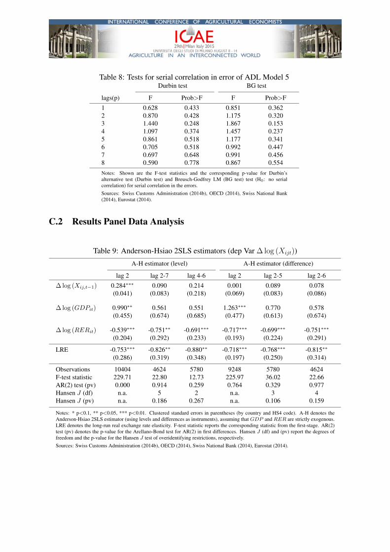
Table 8: Tests for serial correlation in error of ADL Model 5Durbin test BG test

lags(p) F Prob>F F Prob>F

1 0.628 0.433 0.851 0.3622 0.870 0.428 1.175 0.3203 1.440 0.248 1.867 0.1534 1.097 0.374 1.457 0.2375 0.861 0.518 1.177 0.3416 0.705 0.518 0.992 0.4477 0.697 0.648 0.991 0.4568 0.590 0.778 0.867 0.554

Notes: Shown are the F-test statistics and the corresponding p-value for Durbin’salternative test (Durbin test) and Breusch-Godfrey LM (BG test) test (H0: no serialcorrelation) for serial correlation in the errors.Sources: Swiss Customs Administration (2014b), OECD (2014), Swiss National Bank(2014), Eurostat (2014).

C.2 Results Panel Data Analysis

Table 9: Anderson-Hsiao 2SLS estimators (dep Var ∆ log (Xijt))

A-H estimator (level) A-H estimator (difference)

lag 2 lag 2-7 lag 4-6 lag 2 lag 2-5 lag 2-6

∆ log (Xij,t−1) 0.284∗∗∗ 0.090 0.214 0.001 0.089 0.078(0.041) (0.083) (0.218) (0.069) (0.083) (0.086)

∆ log (GDPit) 0.990∗∗ 0.561 0.551 1.263∗∗∗ 0.770 0.578(0.455) (0.674) (0.685) (0.477) (0.613) (0.674)

∆ log (RERit) -0.539∗∗∗ -0.751∗∗ -0.691∗∗∗ -0.717∗∗∗ -0.699∗∗∗ -0.751∗∗∗

(0.204) (0.292) (0.233) (0.193) (0.224) (0.291)

LRE -0.753∗∗∗ -0.826∗∗ -0.880∗∗ -0.718∗∗∗ -0.768∗∗∗ -0.815∗∗

(0.286) (0.319) (0.348) (0.197) (0.250) (0.314)

Observations 10404 4624 5780 9248 5780 4624F-test statistic 229.71 22.80 12.73 225.97 36.02 22.66AR(2) test (pv) 0.000 0.914 0.259 0.764 0.329 0.977Hansen J (df) n.a. 5 2 n.a. 3 4Hansen J (pv) n.a. 0.186 0.267 n.a. 0.106 0.159

Notes: * p<0.1, ** p<0.05, *** p<0.01. Clustered standard errors in parentheses (by country and HS4 code). A-H denotes theAnderson-Hsiao 2SLS estimator (using levels and differences as instruments), assuming that GDP and RER are strictly exogenous.LRE denotes the long-run real exchange rate elasticity. F-test statistic reports the corresponding statistic from the first-stage. AR(2)test (pv) denotes the p-value for the Arellano-Bond test for AR(2) in first differences. Hansen J (df) and (pv) report the degrees offreedom and the p-value for the Hansen J test of overidentifying restrictions, respectively.Sources: Swiss Customs Administration (2014b), OECD (2014), Swiss National Bank (2014), Eurostat (2014).

Table 10: Arellano-Bond one-step difference GMM estimators (dep Var ∆ log (Xijt))

all collapsed lag5 lag6to7 lag6to8 lag7to8 lag6to9 lag7to9

∆ log (Xij,t−1) 0.305∗∗∗ 0.317∗∗∗ 0.374 0.360 0.224 0.162 0.215 0.244(0.035) (0.038) (0.296) (0.250) (0.209) (0.381) (0.210) (0.379)

∆ log (GDPit) 1.681∗∗∗ 1.144∗∗ 0.915 0.900 1.101∗∗ 1.179∗ 1.109∗∗ 1.058(0.472) (0.461) (0.616) (0.566) (0.529) (0.716) (0.530) (0.707)

∆ log (RERit) -0.549∗∗∗ -0.561∗∗∗ -0.526∗∗ -0.525∗∗ -0.547∗∗∗ -0.559∗∗∗ -0.548∗∗∗ -0.545∗∗

(0.203) (0.207) (0.221) (0.218) (0.204) (0.206) (0.203) (0.212)

LRE -0.790∗∗∗ -0.822∗∗∗ -0.840∗ -0.820∗∗ -0.705∗∗ -0.667∗∗ -0.698∗∗ -0.721∗

(0.293) (0.303) (0.446) (0.397) (0.289) (0.322) (0.285) (0.377)

Observations 10404 10404 10404 10404 10404 10404 10404 10404No Instruments 56 20 16 18 20 16 21 17AR(2) test (pv) 0.000 0.000 0.127 0.100 0.191 0.559 0.208 0.403Hansen J (df) 44 8 4 6 8 4 9 5Hansen J (pv) 0.000 0.029 0.101 0.185 0.135 0.234 0.176 0.285

Notes: * p<0.1, ** p<0.05, *** p<0.01. Cluster-robust standard errors in parentheses. Arellano-Bond one-step difference GMMestimator, assuming that GDP and RER are strictly exogenous. All models include year dummies. LRE denotes the long-run realexchange rate elasticity. AR(2) test reports the p-value for the Arellano-Bond test for AR(2) in first differences. Hansen J (df) and(pv) report the degrees of freedom and the p-value for the Hansen J test of overidentifying restrictions, respectively.Sources: Swiss Customs Administration (2014b), OECD (2014), Swiss National Bank (2014), Eurostat (2014).