Exchange Rate Prediction using Support

Vector Machines

A comparison with Artificial Neural Networks

Thesis submitted in partial fulfillment of the requirements for the degree of MASTER OF SCIENCE IN MANAGEMENT OF TECHNOLOGY

AUTHOR Mohamad Alamili 1286676

JANUARY, 2011 DELFT UNIVERSITY OF TECHNOLOGY Faculty of Technology, Policy and Management Section of Information and Communication Technology GRADUATION COMMITTEE Chairman Prof. dr. Y.H. Tan 1st Supervisor Dr. ir. J. van den Berg Daily Supervisor M. Davarynejad 2nd Supervisor J. Vrancken

2

Acknowledgments

There are many people without whom this master’s thesis would not have been possible. It is, in fact, difficult to fully acknowledge their support towards me and towards this work. Nonetheless, I would like to take the opportunity to express my gratitude towards them. First and foremost, I would like to express my deepest gratitude to my first supervisor Dr.ir. Jan van den Berg, for his continuous support and guidance in writing this thesis, and for his patience, motivation, enthusiasm, and immense knowledge that has helped me tremendously. I have been amazingly fortunate to have a supervisor who gave me the freedom to explore on my own, and at the same time the guidance to overcome many difficult situations as they presented. Not only did I enjoy our discussions on related topics that helped me improve my knowledge in the area, but also the numerous personal talks that we had at almost each time that we met.

I would like to extend my gratitude to the rest of my thesis committee: Prof. dr. Y.H. Tan, Mohsen Davarynejad, and Jos Vrancken. Without their support, this thesis could not have been possible. Special gratitude goes to Mohsen, who provided me with insightful comments and constructive criticisms at different stages of my thesis. I am also grateful to him for holding me to a high research standard and enforcing strict validations for each research result, for encouraging the use of correct grammar and consistent notation in my writings, and for carefully reading and commenting on countless revisions of this thesis. I would like to thank Jos for sharing his knowledge and expertise in mathematics, and explaining me the basics where I did not understood them correctly. His sharp revisions on my writing has also been greatly appreciated. Furthermore, I warmly appreciate the generosity, support, patience, and understanding from my girlfriend Sabine de Ridder. Without her countless times of helping my writing, this thesis would not have been possible. In all, for taking care of me. I would also like to thank all my friends for their support and companionship, and all my fellow students, those who directly and indirectly supported me in completing my thesis and my study, and who made my studies in Delft and Singapore an enjoyable and unforgettable experience.

Most importantly, none of this would have been possible without the love and patience of my family. My immediate family to whom this thesis is dedicated to, including my mother Ahlam Alfattal, my father Adnan Alamili, my sisters Aseel Alamili and Zaman Alamili, and my brother in law and true friend, Amar Alambagi. They all have been a constant source of love, concern, support and strength. I would like to express a special heart-felt gratitude to my mother, for her continuous support throughout my entire studies, and for believing in my capabilities, at times more than I believed in myself. Most importantly, for making me who I am.

Mohamad Alamili,

Den Haag 2011

3

Table of Contents

Executive Summary ................................................................................................................ 5

1 Introduction .................................................................................................................... 6

1.1 Research Problem ......................................................................................................... 7

1.2 Research Objective ....................................................................................................... 9

1.3 Research Approach ...................................................................................................... 11

2 Conceptualization of financial forecasting ......................................................................... 14

2.1 Financial markets ........................................................................................................ 14

2.2 Is it possible to forecast financial markets? .................................................................... 15

2.3 Traditional forecasting techniques for the currency market ............................................. 17

2.3.1 Fundamental analysis .........................................................................................................17

2.3.2 Technical analysis ...............................................................................................................17

2.4 Conclusions ................................................................................................................ 19

3 Computational Intelligence Techniques used ..................................................................... 20

3.1 Artificial Neural Network .............................................................................................. 20

3.1.1 The Multilayer Perceptron Neural Network ....................................................................... 20

3.1.2 Application of Artificial Neural Networks in financial forecasting ....................................... 23

3.2 Support Vector Machines ............................................................................................. 24

3.2.1 The Theory of Support Vector Machines: Classification ..................................................... 24

3.2.2 The Theory of Support Vector Machines: Regression ........................................................ 31

3.2.3 Application of Support Vector Machines ............................................................................ 33

3.3 Conclusions ................................................................................................................. 33

4 Design of the Prediction Models .......................................................................................36

4.1 Input Selection ............................................................................................................36

4.1.1 Sampling ........................................................................................................................... 37

4.1.2 Transforming .................................................................................................................... 39

4.1.3 Normalizing ....................................................................................................................... 40

4.1.4 Dividing ............................................................................................................................. 42

4.1.5 Windowing ........................................................................................................................ 42

4

4.2 Output Selection ......................................................................................................... 43

4.2.1 Performance measures .................................................................................................. 43

4.3 The bias-variance dilemma ........................................................................................... 45

4.4 The SVM model selection ............................................................................................. 47

4.4.1 The SVM architecture .................................................................................................... 47

4.4.2 The SVM kernel .............................................................................................................. 53

4.5 ANN Model Selection ...................................................................................................56

4.5.1 Neurodynamics of the network ..................................................................................... 56

4.5.2 Architecture of the network ........................................................................................... 57

4.6 Conclusions .................................................................................................................59

5 Experimentation ............................................................................................................ 62

5.1 Experimental setup .................................................................................................... 62

5.2 SVM experiments ........................................................................................................63

5.3 ANN experiment .........................................................................................................67

5.4 Detailed analysis of the experimental results ................................................................ 69

6 Reflection ....................................................................................................................... 72

7 Conclusions .................................................................................................................... 74

7.1 Answers to the Research Questions .............................................................................. 74

7.2 Limitations ................................................................................................................. 77

7.3 Future Research ......................................................................................................... 78

References ........................................................................................................................... 80

5

Executive Summary

Financial forecasting in general, and exchange rate prediction in particular, is an issue of much interest

to both academic and economic communities. Being able to accurately forecast exchange rate

movements provides considerable benefits to both firms and investors. This research aims to propose

a decision support aid to these firms and investors, enabling them to better anticipate on possible

future exchange rate movements, based on one of the most promising prediction models recently

developed within computational intelligence, the Support Vector Machine.

The economics of supply and demand largely determine the exchange rate fluctuations. Calculating the

supply and demand curves to determine the exchange rate has shown to be unfeasible. Therefore, one

needs to rely on various forecasting methods. The traditional linear forecasting methods suffer from

their linear nature, since empirical evidence has demonstrated the existence of nonlinearities in

exchange rates. In addition, the usefulness of the parametric, and nonparametric, nonlinear models,

has shown to be restricted. For these reasons, the use of computational intelligence in predicting the

Euro Dollar exchange rate (EUR/USD) is investigated, in which these previously mentioned limitations

may be overcome. The methods used are the Artificial Neural Network (ANN) and the Support Vector

Machine (SVM).

The ANN, more specifically the Multilayer Perceptron, is composed of several layers containing nodes

that are interconnected, allowing the neurons to signal each other as information is processed. The

basic idea of the SVM is finding a maximum margin classifier that separates a training set between

positive and negative classes, based on a discriminant function that maximizes the geometric margin.

The model selection for the prediction models was chosen to be based on the bias-variance dilemma,

which denotes the trade-off between the amount of variation within different estimators on different

values of a specific data set (variation) and the difference between the estimator’s expected value and

the true value of the parameter being estimated (bias). Experiments on the Mackey-Glass dataset and

on the EUR/USD dataset have yielded some appropriate parameter ranges for the ANN and SVM.

On theoretical grounds, it has been shown that SVMs have a few interesting properties which may

support the notion that SVMs generally perform better than ANNs. However, on empirical grounds,

based on experimentation results in this research, no solid conclusion could be drawn regarding which

model performed the best on the EUR/USD data set. Nevertheless, in light of providing firms and

investors the necessary knowledge to act accordingly on possible future exchange rate movements, the

SVM prediction model may still be used as a decision-support aid for this particular purpose. While the

predictions on their own as provided by the SVM are not necessarily accurate, they may provide some

added value in combination with other models. In addition, users of the model may learn to interpret

the predictions in such a way, that they still signal some sort of relevant information.

6

1 Introduction

With an estimated $4.0 trillion (Bank of International Settlements, 2010) average daily turnover, the

global foreign currency exchange market is undoubtedly considered the largest and most liquid of all

financial markets. The exchange market is a complex, nonlinear, and a dynamic system of which its

time series, represented by the exchange rates, are inherently noisy, non-stationary, non-linear, and of

an unstructured nature. (Hall, 1994; Taylor, 1992; Yaser et al., 1996). These characteristics, combined

with the immense trading volume and the many correlated influencing factors of economic, political,

and psychological nature, has made exchange rate prediction one of the most difficult and demanding

applications of financial forecasting (Beran, 1999; Fernandez-Rodriguez, 1999).

For large multinational firms, which regard currency transfers as an important aspect within their

business, as well as for firms of all sizes that import and export products and services, being able to

accurately forecast exchange rate movements provides a considerable enhancement in the firm’s

overall performance and profitability (Rugman and Collinson, 2006). In addition to firms, both

individual and institutional investors benefit from an exchange rate prediction as well (Dunis, 2008).

The firms and investors will on one hand be able to effectively hedge themselves against potential

market risks, while on the other hand have the means to create new profit making opportunities. The

aim of this research is aiding firms and investors with the necessary knowledge to better anticipate on

possible future exchange rate movements. The motivation for this research is to apply one of the most

promising prediction models recently developed, being the Support Vector Machine (Vapnik, 1995), to

assess whether it can achieve a high performance in exchange rate prediction.

This thesis consists of seven chapters and is organized as follows. This first chapter describes the

research problem, formulates the research objective and questions, and explains the research approach.

Chapter 2 dives into the philosophy of financial forecasting and provides a basic understanding of the

traditional forecasting methods. Chapter 3 explores the application of Computational Intelligence in

financial forecasting, particularly that of Support Vector Machines and Artificial Neural Networks.

Chapter 4 describes the design of the Support Vector Machine and the Artificial Neural Network for the

purpose of exchange rate prediction. Chapter 5 outlines the experiment methodology and discusses the

empirical results. Chapter 6 reflects on these results with respect to the original research objective and

questions. Finally, chapter 7 presents the conclusions, limitations, and future research.

7

1.1 Research Problem

Financial forecasting in general, and exchange rate prediction in particular, is an issue of much interest

to both academic and economic communities (Lento et al.,2007). Within the academic community,

forecasting by prediction models is an important and widely studied topic employing various statistical

methods and data mining techniques. These methods include, but are not limited to, Regression

Analysis, Discriminate Analysis, Logistic Models, Factor Analysis, Decision Trees, Artificially Neural

Networks (ANN), Fuzzy Logic, Genetic Algorithms, and Support Vector Machines (SVM) (Kecman,

2001). These so-called ‘computational intelligence’ models within the realm of soft computing, have

often shown to be quite successful in financial forecasting which includes forecasting interest rates,

stock indices, currencies, creditworthiness, or bankruptcy prediction (Zhang et al., 1997). They are

however not limited to financial forecasting, but have been applied by many research institutions to

solve many diverse types of real world problems in pattern classification, time series forecasting,

medical diagnostics, robotics, industrial process control, optimization, and signal processing (Kecman,

2001).

Within the economic community, the interest in exchange rate prediction originates from the benefits

of being able to better anticipate future movements, be it for financial gain or protecting against

certain risks (Liu et al.,2007). For instance, large multinational firms consider currency transfers as an

important aspect within their business and may benefit greatly from an accurate forecasting (Rugman

and Collinson, 2006). However, this interest in the exchange market is not limited to large multinational

firms. In fact, exchange rate prediction is relevant to all sorts of firms, disregarding its size, geographic

dispersion, or core business. The reason is that whether or not a firm is directly involved in international

business through imports, exports, and direct foreign investment, its purchases of imported products or

services may require payment in a foreign currency. As a consequence, the prices of imported or

exported products and services may vary with the exchange rate, introducing a certain exchange risk.

This exchange risk is defined as the possibility that a firm will be unable to adjust its prices and costs to

exactly offset exchange rate changes (Rugman and Collinson, 2006). Even if a domestic firm does not

import or export products and services, it might still face this risk, since suppliers, customers, and

competitors that are doing international business will adjust to the exchange rate changes, which will in

turn affect the domestic firm as well. Apart from importing and exporting goods, a firm may choose to

invest in a foreign business or security, and face both different interest rates and different risks from

those at the home country. For instance, borrowing funds abroad may appear interesting if it is less

expensive and under better terms than borrowing domestically, yet it still introduces an exchange risk.

There are certain measures that allow a firm to minimize its exchange risk. These measures range from

trying to avoid foreign currency transactions to currency diversification and all methods of ‘hedging’

against exchange rate changes (Rugman and Collinson, 2006). Independent of the firm's strategy to

minimize the exchange risk, being able to accurately predict exchange rate movements may reduce the

exchange risk significantly (Dunis and Williams, 2002). Literature provides many methods to predict the

financial markets in general and the exchange rate market in particular, which is conducted by either

technical analysis or fundamental analysis (Bilson, 1992; LeBaron, 1993; Levich & Thomas, 1993; Taylor

8

1994). Technical analysis bases the prediction only on historical prices, whereas fundamental analysis

bases it on macro- and microeconomic factors. Traditional methods within technical analysis, such as

common market structure trading rules and the ARIMA method, have been empirically tested in an

attempt to determine their effectiveness on different financial securities such as currencies, with

varying success (Brock, Lakonishok, and LeBaron, 1992; Chang and Osler, 1994; Lo and MacKinley,

1999).

Computational intelligence techniques for exchange rate prediction has gained a lot of popularity the

last 15 years, especially with ANNs, that has been widely used for this purpose and in many other

different fields of business, science, and industry (Bellgard and Goldschmidt, 1999; El Shazly and El

Shazly, 1997; Yao et al., 1997; Widow et al., 1994). The common element of computational intelligence

techniques is generalization through nonlinear approximation and interpolation in usually high-

dimensional spaces (Kecman, 2001). It is the power of their generalization ability, producing outputs

from unseen inputs through captured patterns in previously learned inputs, what makes these

techniques excellent classifiers and regression models (Kecman, 2001). This partly explains their

increased popularity in this field and distinguishes them from the previously mentioned traditional

methods.

Recently, a new technique within the field of computational intelligence, that of Support Vector

Machines (SVM), has been applied to financial markets. In the current literature, these have often

shown to be more effective than ANNs (Kim, 2003; Thissen et al., 2003; Liu and Wang, 2008). The SVM,

which has been introduced by Vapnik and coworkers in 1992, is a noticeable and prominent classifier

and perfectly able to solve nonlinear regression estimation problems. However, it has been shown that

the prediction performance of SVMs are very sensitive to the value of its parameters, being the value of

soft-margin constant and various kernel parameters (Kim, 2002). The very few researchers that

examined the feasibility of SVMs applied to exchange rate prediction, have chosen these parameters

for being the most effective on the used data set (Liu and Wang 2008; Tay et al., 2000; Thissen et al.,

2003).

In this research, the focus is on employing an SVM for the purpose of exchange rate prediction, meant

as a decision-support aid to firms and investors. The contribution of this research is to identify the best

performing SVM in terms of model structure and parameters on a given exchange rate, being the

EUR/USD exchange rate. The performance of the SVM will be compared to that of an ANN on the used

exchange rate data set.

9

1.2 Research Objective

The main research objective is formulated as follows:

This research aims to propose a prediction model that is able to accurately predict exchange rate

movements, thereby acting as a decision-support aid for firms and investors, providing them the necessary

knowledge to better anticipate possible future exchange rate movements.

This objective is very broad in the sense that there are many definitions of predicting, many kinds of

prediction models, and many variations of the exchange rate market. This research focuses on a narrow

range of solutions to fulfill this objective, which will be given subsequently.

Regarding predicting, it should be stressed at this earliest moment that the focus of this research is

developing a prediction model that is useful for firms and investors, yet not necessarily a profitable

trading model. In a relatively slow-moving market, accurate prediction models may well equate to a

profitable trading model (Bodt et al., 2001). However, within a high-frequency data environment, such

as the exchange rate market, having an accurate prediction model does not necessarily lead to

achieving profitable trading results (Cao and Tay, 2000). To benefit financially from an accurate

prediction, one needs to take a trading strategy into account with all the associated transaction costs,

which is a much more complicated task (Chordia and Shivakumar, 2000). In this sense, the aim of this

research is to develop a decision-support aid by which the achievable profitability is inferred from the

extent of prediction errors, rather than measured directly. For instance, a prediction model in this

research is regarded to be useful for firms and investors when the prediction errors are relatively small,

without actually having measured the gain in profits due to the predictions. The firms and investors are

then able to act accordingly on these predictions by buying or selling a specific currency based on the

predicted probability that this specific currency will rise, fall, or remain unchanged. For instance, if a

French firm is seeking to import goods from the United States, which requires a currency exchange

from euros to dollars, it may decide to do so when the euro dollar exchange rate is predicted to rise, for

which the French firm will receive more dollars per euro and thereby reducing the import costs.

Another point regarding predicting, is whether it is conducted by either technical analysis or

fundamental analysis, as mentioned before. Technical analysis bases its prediction only on historical

data such as past prices or volumes, whereas fundamental analysis bases its prediction on macro- and

microeconomic factors that might determine the underlying causes of price movements, such as the

interest rate and the employment rate (Bilson, 1992; LeBaron, 1993; Levich & Thomas, 1993; Taylor

1994). This research will solely focus on technical analysis, and not on fundamental analysis. The

motivation behind this choice is that technical analysis is the most commonly used method of

forecasting by investment analysts in general and foreign exchange dealers in particular (Taylor and

Allen, 1992; Carter and Auken, 1990). Technical analysis is also more often applied than fundamental

analysis when one is mostly interested in the short-term movements of currencies (Robert, 1999).

Within technical analysis, only past exchange rates will be investigated, since volume is not available in

the exchange rate market.

10

Concerning the exchange rate market, the Euro Dollar exchange rate (EUR/USD) will be the currency

pair subjected to forecasting. This is a matter of choice, partly justified by being the most traded

currency pair in the world, and partly by the very specific interest this currency pair has raised in the

literature of financial forecasting by means of computational intelligence (Dunis et al., 2008).

As described earlier, there are many prediction models currently available. Within the scope of this

research, only models based on computational intelligence will be investigated, namely the SVM and

the ANN. A comparison will be made between the SVM and the ANN, while the focus will be more on

the SVM. The reason why only computational intelligence techniques are used in this research is

because of the earlier mentioned characteristics that they possess which distinguished them from the

other previously mentioned traditional methods and increased their popularity in financial forecasting

over the last decade. These characteristics revolve around generalization through nonlinear

approximation and interpolation in usually high-dimensional spaces. (Kecman, 2001). The power of

their generalization ability, producing outputs from unseen inputs through captured patterns in

previously learned inputs, makes them excellent classifiers and regression models (Kecman, 2001).

Based on the aforementioned, the main research question is formulated as follows:

"What is the practical feasibility in terms of prediction accuracy of a Support Vector Machine compared to

an Artificial Neural Network for the purpose of exchange rate prediction?"

As can be noted, the comparison criteria between the SVM and the ANN is solely based on prediction

accuracy. Other possible comparison criteria are computational complexity and speed. However, in this

research, these comparison criteria are not taken into account. The reason for this choice is that for the

purpose of the decision-support aid as proposed in this research, prediction accuracy is the most crucial

element which will always be the deciding factor, even if it means slower speed or higher

computational complexity. In addition, earlier research has shown that the speed between the SVM and

the ANN in operational mode is neglectable for the decision-support aid as proposed in this research,

since the speed difference is merely seconds to minutes rather than hours (LeCun et al.,1995).

Furthermore, previous research concerning financial forecasting usually does not take speed into

account, since accuracy is again far more relevant than speed in these situations (Huang et al., 2004).

In order to answer the main research question, experiments need to be conducted for both an SVM and

an ANN to predict the EUR/USD exchange rate movements, by which both results can be compared to

each other and a conclusion can be drawn. In order to arrive at these experiments and the conclusion,

the main question will be approached by answering the following subquestions:

1. What are the options for exchange rate prediction?

2. What is the input selection for the SVM and the ANN, and how is this input preprocessed?

3. What is the output selection for the SVM and the ANN, and how is this output interpreted?

4. How to approach the model selection for both the SVM and the ANN?

5. Which model performed best in predicting the EUR/USD exchange rate movements?

11

The subquestions will lead to the answer of the main research question in a chronological order. Firstly,

the possibilities of exchange rate prediction are examined. This will not only provide information

regarding the exchange rate market and its predictability, but it will also provide insights into the

second subquestion, i.e. data preprocessing suitable for financial markets. The output selection as in

third sub question will be based on the main research question, by measuring the feasibility of a specific

model assessed through the prediction accuracy. The fourth subquestion describes how different

models are constructed by different influencing parameters, based on the model complexity and

expressed in the bias-variance dilemma, as will be explained later in Chapter 4. The final subquestion is

obtained by doing experiments on a range of suitable models and drawing a conclusion on these

experimental results.

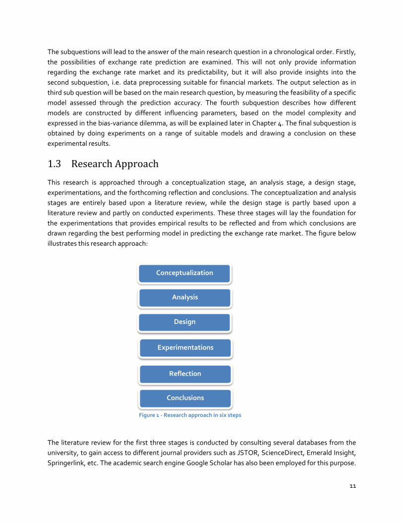
1.3 Research Approach

This research is approached through a conceptualization stage, an analysis stage, a design stage,

experimentations, and the forthcoming reflection and conclusions. The conceptualization and analysis

stages are entirely based upon a literature review, while the design stage is partly based upon a

literature review and partly on conducted experiments. These three stages will lay the foundation for

the experimentations that provides empirical results to be reflected and from which conclusions are

drawn regarding the best performing model in predicting the exchange rate market. The figure below

illustrates this research approach:

The literature review for the first three stages is conducted by consulting several databases from the

university, to gain access to different journal providers such as JSTOR, ScienceDirect, Emerald Insight,

Springerlink, etc. The academic search engine Google Scholar has also been employed for this purpose.

Conceptualization

Analysis

Reflection

Experimentations

Conclusions

Design

Figure 1 - Research approach in six steps

12

In addition, both references from colleagues as well as references in the articles found have been

reviewed.

The search keywords used include: financial markets, financial forecasting, currency market, foreign

exchange, forecasting techniques, computational intelligence, support vector machines, neural networks,

multilayer perceptrons, genetic algorithms, hybrid models of computational intelligence, regression models

The aim of the conceptualization stage is to understand the fundamental subjects related to financial

forecasting through a literature study. Firstly, a brief description of financial markets in general and the

exchange market in particular is provided. Secondly, it is examined to what extent financial forecasting

is considered possible according to different academics in this field. Thirdly, different traditional

methods for forecasting the financial markets are given, which may provide valuable insight in how the

more advanced computational intelligence techniques can be applied to exchange rate prediction.

The analysis stage follows up on the philosophy of financial forecasting in the conceptualization stage,

by presenting some of the most popular financial forecasting techniques, both within and without the

field of computational intelligence. While doing so, the focus will be mostly on the currency market and

mostly on technical analysis techniques, to be more in line with the focus of this research. It is

noteworthy to mention that it is out of the scope of this research to provide an extensive overview of all

the computational intelligence techniques in financial forecasting. Therefore, this stage is limited to the

exploration of ANNs and SVMs. Nevertheless, the underlying theory behind SVMs and ANNs is

described, in which the bare basics are briefly introduced, necessary to effectively apply these models in

financial forecasting. In addition, the application of these models in financial forecasting by earlier

research is examined.

Following the analysis stage is the design stage, which, in addition to further literature review and

certain experiments, incorporates the knowledge acquired from the previous stages to outline the

design for the SVM and the ANN. The design stage starts with the input selection, in which the

processing steps to prepare the raw data to a suitable input for the models are investigated. This

processing will be broken down into five steps (Huang et al., 2004):

1. Sampling

2. Transforming

3. Normalizing

4. Dividing

5. Windowing

For each step, it is investigated what the possible choices are, based on a literature review, and what

specific processing will be chosen for in this research. A visual representation on the EUR/USD data set

is presented after certain processing steps, to illustrate that particular processing step.

13

Following is the output selection, that determines the output of the models and how this output is

interpreted. Different choices regarding the output selection of the models is investigated and a

specific output appropriate to the focus of this research is selected. In addition, different performance

measures will be examined. The performance measures should be comparable between the ANN and

the SVM, in order to draw a conclusion which of the two performs better.

Subsequently, the model selection for the ANN and the SVM is examined. The aim is to identify a

suitable range for the parameters that yields a balanced model in terms of model complexity. The

model complexity will be expressed in the bias-variance dilemma.

The results in the design stage will provide an appropriate range for certain parameters that serve as a

starting point for the experimentations. As a result of the experimentations, the best SVM and the best

ANN is identified through a grid search on the parameter range, based on a certain performance

measure. These results are then reflected upon, by which after A conclusion is drawn regarding how the

SVM has performed in comparison to the ANN. Subsequently, the limitations of this research and

possible future research is given.

14

2 Conceptualization of financial forecasting

This chapter presents the fundamental understanding of subjects related to financial forecasting

through a literature study. In the first section, a brief description of financial markets in general and the

exchange market in particular is provided. The second section examines different views regarding

whether financial forecasting is possible or not. Afterwards, different traditional methods for

forecasting the financial markets are given, which may provide valuable insight into how the more

advanced computational intelligence techniques can be applied to exchange rate prediction.

2.1 Financial markets

A necessary precondition for financial forecasting is an understanding of financial markets and the data

that is derived from these markets. This section starts with explaining what is meant by a financial

market in the broader term, and by a currency market in the specific term.

A financial market is a mechanism that allows people to buy and sell financial securities and

commodities, to facilitate the raising of capital in capital markets, the transferring of risk in derivatives

markets, or the international trading in currency markets (Pilbeam, 2010). These securities and

commodities come in many different kinds. For instance, the classical share is a popular security that

represents a piece of ownership of a firm and which is exchanged on the stock market. Other popular

securities are bonds, currencies, futures, options and warrants.

All of these financial securities are traded every day on specific financial markets with specific rules

governing their quotation (Bodt et al., 2001). However, quotation is not the only financial data that can

be retrieved from a financial market. The trading volume or the amount of dividends of a specific share

can provide valuable information regarding that share’s value. Moreover, not all financial data are

retrieved from the financial markets, data can also be retrieved from financial statements, forecasts

from a financial analysts, etc. It is out of the scope of this research to cover all these kinds of financial

securities with all the different financial data. The focus of this research concentrates on the currency

market, more specifically the EUR/USD currency market.

The global foreign currency market is undoubtedly considered the largest and most liquid of all financial

markets, with an estimated average daily turnover of $4.0 trillion (Bank of International Settlements,

2010). Currencies are traded in the form of currency pairs through a transaction between one country's

currency and another's. These transactions are not limited to the exchange of currencies printed by a

foreign country's central bank, but also includes checks, wire transfers, telephone transfers, and even

contracts to sell or buy currency in the future (Rugman and Collinson, 2006). These different

transactions are facilitated through four different markets, which include the spot market, the futures

market, the options market, and the derivatives market (Levinson, 2006). All these different markets

function separately but are yet closely interlinked.

15

The spot market facilitates an immediate delivery for the currencies to be traded, while the future and

option markets allow participants to lock in an exchange rate at a certain future date by buying or

selling a futures contract or on option. The most trading in the currency market now occurs in the

derivatives market, which accounts for the forward contracts, foreign-exchange swaps, foreign rate

agreements and barrier options (Levinson, 2006). These currency markets are highly distributed

geographically and have no single physical location. Most trading occurs in the interbank markets

among financial institutions across the world. The participants in the currency market are composed of

exporters and importers, investors, speculators and governments. The most widely traded currency is

the US dollar, while the most popular currency pair is the EUR/USD (Bank of International Settlements,

2010).

The price of a specific currency is referred to as the exchange rate, which also accounts for the spread

established by the participants in the market. The economics of supply and demand largely determine

the exchange rate fluctuations (Rugman and Collinson, 2006). Ideally, one would determine the

exchange rate by calculating supply and demand curves for each exchange market participant and

anticipate government constraints on the exchange market. However, this information is lacking due to

the immense size of the exchange market, by which calculating the supply and demand curve for each

participant is simply unfeasible. This is the reason why there is no certainty in determining the

exchange rate and therefore one needs to rely on various forecasting models, being either fundamental

or technical forecasting methods, which will be explained in the next section.

For more information regarding the currency market, readers are referred to The guide to financial

markets by Mark Levinson (2006). However, for the sole purpose of this research, no further in-depth

information concerning the currency market is required.

2.2 Is it possible to forecast financial markets?

There are many typical applications of forecasting in the financial world, e.g. simulation of market

behavior, portfolio selection/diversification, economic forecasting, identification of economic

explanatory variables, risk rating of mortgages, fixed income investments, index construction, etc.

(Trippi et al., 1992). The main question remains however, to what extent financial markets are

susceptible to forecasting? Literature shows that opposing views exist between academic communities

on whether financial markets are susceptible to forecasting, which are described below.

Fama (1965) presents empirical tests of the random walk hypothesis, that was first proposed by

Bachelier in 1900. The random walk hypothesis states that past stock prices are of no real value in

forecasting future prices because past, current, and future prices merely reflect market responses to

information that comes into the market at random (Bachelier, 1900). Fama’s conclusion (1965) based

on empirical tests is: “the main conclusion will be that the data seem to present consistent and strong

support for the random walk hypothesis. This implies, of course, that chart reading, though perhaps an

interesting pastime, is of no real value to the stock market investor.” However, the statistical tests that

16

Fama performed and that support the notion that financial markets follow a random walk were based

on the discovery that there was no linear dependency in the financial market (Tenti, 1996).

Nevertheless, the lack of a linear dependency did not rule out nonlinear dependencies, which would

contradict the random walk hypothesis. Some researchers argue that nonlinearities do exist in the

currency market (Brock et al., 1991; De Grauwe et al., 1993; Fang et al., 1994; Taylor, 1986).

Fama’s conclusion (1965) is supported by the main theoretical argument of the efficient market

hypothesis. This hypothesis states that a particular market is said to be efficient, if all the participants

and actors related to that market receive all possible information at any time and at the same time

(Malkiel, 1987). As a consequence, the price in such a market will only move at the arrival of new

information, which is by definition impossible to forecast on historical data only. Nevertheless, despite

this reason why financial forecasting is criticized by many economists, most notably by Malkiel (1995),

financial forecasting has still received an increasing amount of academic attention. It has been shown

by some researchers that financial forecasting does hold a predictive ability and profitability by both

technical analysis and fundamental analysis (Sweeney, 1988; Brock., Lakonishok, LeBaron, 1992;

Bessembinder and Chan, 1995; Huang, 1995; Raj and Thurston, 1996). While this shows that evidence

has been found of predictive ability by financial forecasting, it does, however, not always provide

profitability when appropriate adjustments are made for risk and transaction costs (Corrado and Lee,

1992; Hudson et al., 1996; Brown et al., 1995; Bessembinder and Chan, 1998; Allen et al., 1999).

In addition, it is questionable whether the financial markets can be portrayed as an ideal representation

of an efficient market. That financial markets are not so efficient is supported by Campbell, the Lo and

MacKinley (1997) in which they state: “Recent econometric advances and empirical evidence seem to

suggest that financial asset returns are predictable to some degree”. One of those econometric

advances has been conducted by Brock, Lakonishok and Le Baron in 1992. They used a bootstrap

methodology to test the most popular technical trading rules on the Dow Jones market index for the

period 1897 to 1986. They concluded that their results provide strong support for market predictability.

Sullivan, Timmerman and White (1999) showed new results on that same data set, extended with 10

years of data. Their bootstrap methodology avoided at least to some extent the data snooping bias by

which they were able to confirm that the results of Brock, Lakonishok and Le Baron are still valid. The

concept of the data snooping bias appears as soon as a specific data set is used more than once for

purposes of forecasting model selection (Lo and MacKinley, 1990). More recently, Lo, Mamaysky and

Wang (2000) showed that a new approach based on nonparametric kernel regression was able to

provide incremental market information and may therefore have some practical value.

Based on all the empirical evidence mentioned above, it is at least evident that there is some sort of

interest in trying to forecast the financial markets, and at most safe to consider that it might indeed be

possible. Lastly, it is noteworthy to mention that a clear distinction must be made between successfully

being able to forecast the market and the possibility to gain financially from this forecast. The

difference is in order to gain financially from a forecast, one needs to take a trading strategy into

account with all the associated transaction costs, which is a much more complicated task (Chordia and

Shivakumar , 2000).

17

2.3 Traditional forecasting techniques for the currency market

This section follows up on the philosophy of financial forecasting in the previous two sections by

presenting some of the most popular financial forecasting techniques (without the use of

computational intelligence) for which some show certain successes. Examining these techniques may

provide valuable insight in how the more advanced computational intelligence techniques may be

applied to exchange rate prediction. Many of these so-called traditional forecasting techniques are found

in literature for financial forecasting in general and for forecasting the currency market in particular

(Bilson, 1992; LeBaron, 1993, Levich & Thomas, 1993; Taylor 1994). There exists an important

distinction within these techniques, which entails forecasting by means of fundamental analysis versus

technical analysis (Bodt et al.,2001). Both of these techniques are described in this section, while the

focus is more on technical analysis to be more in line with the focus of his research.

2.3.1 Fundamental analysis

Fundamental analysis is concerned with analyzing the macroeconomic and/or the microeconomic

factors that influence the price of a specific security in order to predict its future movement (Lam,

2004). An example is examining a firm's business strategy or its competitive environment to forecast

whether its share value will rise or decline. In the case of the currency market, one would mostly

examine macroeconomic factors. For instance, the interest rate, the inflation rate, the rate of economic

growth, employment, consumer spending, and other economic variables can have a significant impact

on the currency market (EddelButtel and McCurdy, 1998).

The enormous literature measuring the effects of macro news on the currency market within the field

of fundamental analysis includes Hakkio and Pearce (1985), Ito and Roley (1987), Ederington and Lee

(1995), DeGennaro and Shrieves (1997), Almeida et al. (1998), Andersen and Bollerslev (1998), Melvin

and Yin (2000), Faust et al. (2003), Love and Payne (2003), Love (2004), Chaboud et al. (2004) and Ben

Omrane et al. (2005). However, there exists controversy in the academic literature concerning financial

forecasting in terms of fundamental analysis. A series of papers by Meese and Rogoff (1983) have

shown that forecasting the currency market based on a random walk model perform better than basing

the forecast on microeconomic models. A number of researchers have reinvestigated the papers

proposed by Meese and Rogoff and have generally found it to be robust (Flood and Rose,1995; Cheung

et al., 2005). Nevertheless, some researchers found that they are able to find a strong relationship

between certain macro surprises and exchange rate returns, given that a narrow time window is used

(Anderson et al., 2003).

2.3.2 Technical analysis

Technical analysis involves the prediction of future price movement of a specific financial security based

on only historical data (Achelis, 1995). This data usually consists only of past prices. However, it can also

include other information about the market, most notably volume. Volume refers to the amount of the

trades that has been made in that specific financial market over a specified time period (Cambell et al.,

1997). Technical analysis can either be of qualitative nature or quantitative nature (Achelis, 1995). When

it is of qualitative nature, it aims to recognize certain patterns in the data by visually inspecting the

18

price. When it is of quantitative nature, it aims to base the prediction on analyzing mathematic

representations of the price, e.g. a moving average. Forecasting by means of technical analysis is

commonly used in forecasting the currency market, where the traders that use technical analysis are

mostly interested in the short-term movement of currencies (Taylor and Allen, 1992).

Many technical analysis techniques have been empirically tested in an attempt to determine their

effectiveness. The effectiveness is often explained by the so-called self-fulfilling property that financial

markets may hold, which refers to the phenomena that if a large group is made to believe the market is

going to rise, then that group will most likely act as if the market is truly going to rise, eventually

leading to an actually rise (Sewell, 2007). During the 1990s, the studies on technical analysis techniques

increased, along with the methods used to test them. A selection of the most influential studies that

have provided support for technical analysis techniques include (in no particular order): Jegadeesh and

Titman (1993), Blume, Easley, and O’Hara (1994), Chan, Jegadeesh, and Lakonishok (1996), Lo and

MacKinlay (1997), Grundy and Martin (2001), and Rouwenhorst (1998). Stronger evidence can be found

in Neftci (1991), Brock, Lakonishok, and LeBaron (1992), Chang and Osler (1994), Osler and Chang

(1995), Allen and Karjalainen (1999), Lo and MacKinlay (1999), Lo, Mamaysky and Wang (2000), Gençay

(1999), and Neely and Weller (1999).

One of the first technical analysis techniques are the common market structure trading rules, of which its

indicators monitor price trends and cycles (Pereira, 1999). These indicators include the filter rule, the

moving average crossover rule, Bollinger bands, trading range breakout (TRB), and many more

(Pereira, 1999). Some of these indicators were used in one of the most influential and referenced

studies ever conducted on technical analysis, the studies by Brock, Lakonishok, and LeBaron in 1992. As

mentioned before, Levich and Thomas conducted a related study with the same indicators in 1993 in

which they provided further evidence of the profitability of technical analysis techniques. These

indicators are shortly described below. Readers are referred to Murphy (1999) for a more extensive and

detailed review.

The filter rule is defined by a single parameter, which is the filter size (Ball, 1978). The most basic filter

rules are simply based on the assumption that if a market price rises or declines by a certain percentage

defined by the filter size, then the price is most likely to continue on that direction. The moving average

crossover rule compares to moving averages, mostly a short-run moving average with a long-run

moving average (Appel, 1999). This indicator proposes that if the short run moving average is above the

long run moving average, the price is likely to decline and vice versa. The moment that both averages

cross, is the moment of trend reversal. This is the most basic form of the moving average cross over

rule, while there exists many variations. Bollinger bands are two standard deviations plots above and

below a specific moving average (Murphy, 1999). When the markets exceed one of the trading bands,

the market is considered to be overextended. It is assumed that the market will then often pull back to

the moving average line (Murphy, 2000). The trading range breakout rule is also referred to as resistance

and support levels (Lento and Gradojevic, 2007). The assumption of this indicator is that when the

market breaks out above a resistance level, the market is most likely to continue to rise, while as when a

market breaks through and below a support level, the market is most likely to continue to decline. The

19

resistance level is defined as the local maximum, and the support level is defined as the local minimum

(Brock, Lakonishok, and LeBaron in 1992). The reasoning behind this indicator is that at the resistance

level, intuition would suggest that many investors are willing to sell, while at the support level many

investors are willing to buy. The selling or buying pressure will create resistance or support respectively,

against the price breaking through the level. These common market structure trading rules, together

with other traditional approaches to time series prediction, such as the ARIMA method or the Box-

Jenkins (Box and Jenkins, 1976; Pankratz, 1983), assumed that the data from the financial market is of a

linear nature. However, it is certainly questionable whether this data is indeed linear, as explained

before. As a matter of fact, empirical evidence has demonstrated the existence of nonlinearities in

exchange rates (Fang et al.,1994). In addition, systems in the real world are often nonlinear. (Granger

and Terasvirta, 1993).

In order to cope with the nonlinearity the exchange rates, certain techniques that are nonlinear of

nature have been developed and applied to exchange rate prediction. These include but are not limited

to the bilinear model by Granger and Anderson (1978), the threshold autoregressive model (TAR) by

Tong and Lim (1980), the autoregressive random variance (ARV) model (So et al., 1999), autoregressive

conditional heteroscedasticity (ARCH) model (Engle, 1982; Hsieh, 1989), general autoregressive

conditional heteroskedasticity (GARCH) model (Bollerslev, 1990) , chaotic dynamic (Peel et al., 1995),

and self-exciting threshold autoregressive (Chappel et al., 1996). Readers are referred to Gooijer and

Kumar (1992) for more information regarding these nonlinear models. The problem with these models

however, is that they are parametric nonlinear models, in that they need to be pre-specified, therefore

restricting the usefulness of these models since not all the possible nonlinear patterns will be captured

(Huang et al., 2004). In other words, one particular nonlinear specification will not be general enough to

capture all the nonlinearities in the data. Furthermore, the few nonparametric nonlinear models that

have been investigated and applied to exchange rate prediction, seem unable to improve upon a single

random walk model (Fama,1965) in out of sample predictions of exchange rates (Diebold and Nason,

1990; Meese and Rose, 1991; Mizrach, 1992).

2.4 Conclusions

The economics of supply and demand largely determine exchange rate fluctuations (Rugman and

Collinson, 2006). Calculating the supply and demand curves to determine the exchange rate has shown

to be unfeasible. Therefore, one needs to rely on various forecasting models, being either based on

fundamental or technical analysis. Empirical evidence from the application of these forecasting models

on various financial markets, as well as empirical evidence in favor and against the efficient market

hypothesis, has shown that it is at least evident that there is some sort of interest in trying to forecast

the financial markets, and at most safe to consider that it might indeed be possible. The traditional

linear forecasting methods as presented in this chapter suffer from their linear nature, since empirical

evidence has demonstrated the existence of nonlinearities in exchange rates. In addition, the

usefulness of the parametric and nonparametric nonlinear models has shown to be restricted. For these

reasons, the use of computational intelligence in predicting the exchange rate is investigated, in which

these previously mentioned limitations may be overcome.

20

3 Computational Intelligence Techniques used

Computational intelligence techniques for the purpose of financial forecasting has gained a lot of

popularity the last 15 years, especially with ANNs (Huang et al., 2004; Bellgard and Goldschmidt, 1999;

El Shazly and El Shazly, 1997; Yao al, 1997). This chapter explores two specific computational

intelligence techniques applicable to exchange rate prediction, namely the Artificial Neural Network

and the Support Vector Machine. For both techniques, the theory is briefly described, and the

application to financial forecasting is examined.

3.1 Artificial Neural Network

Artificial Neural Networks (ANN) have been applied in many different fields of business, science, and

industry, to classify and recognize patterns (Widow et al., 1994). They have also been widely used for

financial forecasting (Sharda, 1994). Inspired by the human brain, they are able to learn and generalize

from previous events to recognize future unseen events (Kecman, 2001).

There are many different ANN models currently available. The Multilayer Perceptron (MLP), the

Hopfield networks, and the Kohonen’s self-organizing networks are probably the most popular and

influential models (Zhang, Patuwo, Hu, 1998). In this section, and in the rest of this research, the focus

from the ANN domain is on the MLP (Rumelhart et al., 1986). One reason for this choice is that the

MLP is perhaps the most popular network architecture used in general, and in financial forecasting in

particular (Huang et al., 2004; Kaastra and Boyd, 1996). Another reason is the MLP’s simple

architecture, yet a powerful problem-solving ability (Tay et al., 2000), as well as its relative ease in

implementation (Huang et al., 2004). First, the theory of the MLP is briefly discussed, based on the

book Learning and Soft Computing (Kecman, 2001). Second, the application of ANNs in financial

forecasting is investigated.

3.1.1 The Multilayer Perceptron Neural Network

An MLP is composed of several layers containing nodes. The lowest layer is the input layer where

external data is received. Generally, neural processing will not occur in the input layer. Therefore, the

input layer is not treated as a layer of neural processing units, but merely input units (Kecman,2001).

The highest layer is the output layer where the problem solution is obtained. In the case of predicting

the currency market, the inputs will be the past observations of the exchange rate and the output will

be the future value of the exchange rate. Between the input and output layer, there can be one or more

intermediate layers that are called the hidden layers. See the figure below for a graphical

representation of an MLP.

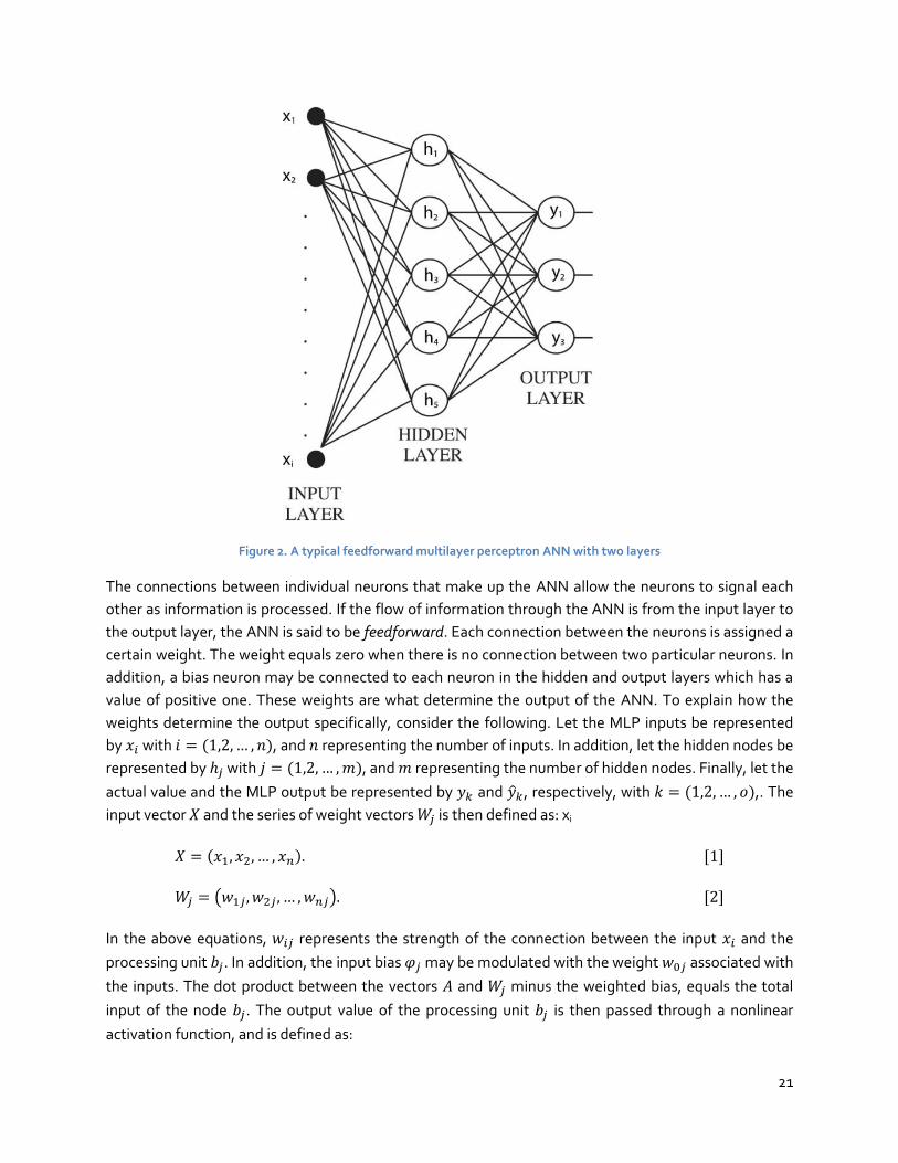
21

Figure 2. A typical feedforward multilayer perceptron ANN with two layers

The connections between individual neurons that make up the ANN allow the neurons to signal each

other as information is processed. If the flow of information through the ANN is from the input layer to

the output layer, the ANN is said to be feedforward. Each connection between the neurons is assigned a

certain weight. The weight equals zero when there is no connection between two particular neurons. In

addition, a bias neuron may be connected to each neuron in the hidden and output layers which has a

value of positive one. These weights are what determine the output of the ANN. To explain how the

weights determine the output specifically, consider the following. Let the MLP inputs be represented

by with , and representing the number of inputs. In addition, let the hidden nodes be

represented by with , and representing the number of hidden nodes. Finally, let the

actual value and the MLP output be represented by and ̂ , respectively, with ,. The

input vector and the series of weight vectors is then defined as: xi

[1]

( ) [2]

In the above equations, represents the strength of the connection between the input and the

processing unit . In addition, the input bias may be modulated with the weight associated with

the inputs. The dot product between the vectors and minus the weighted bias, equals the total

input of the node . The output value of the processing unit is then passed through a nonlinear

activation function, and is defined as:

22

(∑

) ( )

Typically, the activation function introduces a degree of nonlinearity, preventing outputs from reaching

very large values that can thereby paralyze the ANN and inhibit training (Kaastra and Boyd, 1996;

Zhang et al., 1998). To assign certain values to the connection weights suitable for a specific problem,

the ANN needs to undergo a training process. Generally, ANN training methods fall into the categories

of supervised, unsupervised, and various hybrid approaches. This research employs a supervised

training on both the ANN and the SVM. Supervised training is accomplished by feeding the ANN a set

of input patterns while attaching desired responses to those patterns, for which these desired

responses are available throughout the training. A well-known learning algorithm in supervised

training, is the error backpropagation algorithm, resulting in backpropagation networks (Shapiro, 2000).

Backpropagation networks are perhaps the most common multilayer networks, and the most used type

in financial forecasting (Kaastra and Boyd,1996). The specific algorithm requires the activation function

to be differentiable.

The training process may start by assigning random weights, typically through a uniform random initialization inside a specific interval, such as . Consequently, the weights are adjusted and the validity of the ANN is examined in the form of a validation error through the backpropagation learning algorithm. This process can be divided into two phases, namely the propagation phase and the weight update phase. In the propagation phase, a training pattern is fed into the input of the ANN and propagated forward to the output of the ANN in order to generate the propagation's output activations. These output activations are then fed back in the ANN and propagated backwards in order to generate the deltas of the output and hidden neurons, through a so-called delta rule. Following is the weight phase, in which each weight is updated depending on its delta, the input activation, and the learning rate. The learning rate is a ratio that influences the speed and quality of learning. These two phases are repeated until the validation error is within an acceptable limit. An important feature of ANNs is that they are considered to be universal functional approximators,

thus being able to approximate any continuous function to any desired accuracy (Irie and Miyake, 1988;

Hornik et al., 1989; Cybenko, 1989; Funahashi, 1989; Hornik, 1991, 1993). ANNs distinguish themselves

from the earlier mentioned traditional forecasting methods by being able to generalize through

nonlinear approximation and interpolation in usually high-dimensional spaces (Kecman, 2001).

Generalization refers to the capacity of the ANN to provide correct outputs when using data that were

not seen during training. This feature is however not limited to ANNs, but rather a common element of

computational intelligence techniques. It is the power of their generalization ability, producing outputs

from unseen inputs through captured patterns in previously learned inputs, what makes these

techniques excellent classifiers and regression models (Kecman, 2001). This feature is extremely useful

in financial forecasting, since the underlying relationships of the financial market is often unknown or

hard to describe (Zhang, Patuwo, Hu, 1998). Another important feature ANNs, In addition, since ANNs

23

do not require a decisive assumption about the generating process to be made in advance, they are

categorized as non-parametric (nonlinear) statistical methods (White, 1989; Ripley, 1993; Cheng and

Titterington, 1994).

However, one problem with ANNs is that the underlying laws governing the system to be modeled and

from which the data is generated, is not always clear. This is referred to as the black box characteristic

of ANNs (Huang et al., 2004). The black box characteristic is however not limited to ANNs, but often

applicable to other computational intelligence techniques as well, such as the SVM (Thissen et al.,

2003). Other problems with ANNs, as stated by Dunis and Williams (2002), is their excessive training

times and the danger of underfitting and overfitting. The phenomenon of overfitting occurs when the

ANN is trained too long in that its capabilities of generalizing becomes limited, and vice versa for under

fitting. Another problem with ANNs is that it requires a selection of a large number of controlling

parameters, which include relevant input arrivals, hidden layers size, learning rate, etc., for which there

is no structured way or method to obtain the most optimal parameters for a given task (Huang et

al.,2004).

3.1.2 Application of Artificial Neural Networks in financial forecasting

ANNs have been used before in order to forecast the currency market on different exchange rates,

which started early in the beginning of the 1990s. Podding (1993) has compared regression analysis

with ANNs in forecasting the exchange rate between the US Dollar and the Deutsche Mark (USD/DEM).

Refense (1993) has also applied an ANN on the USD/DEM exchange rate, but he has used a constructive

learning algorithm to find the best ANN configuration. Weigend et al. (1992) shows that ANNs perform

better than random walk models in forecasting the USD/DEM exchange rate. Shin (1993) has compared

an ANN model with the moving average crossover rule as described earlier and found that the ANN

performed better. In a similar fashion, Wu (1995) has compared ANNs with the previous mentioned

ARIMA model in forecasting the exchange rate between the Taiwan Dollar and the US Dollar exchange

rate. Refense et al. (1993) have applied a multilayer perceptron ANN to forecast the USD/DEM

exchange rate. More recent applications of ANNs in exchange rate predictions are by Andreou and

Zombanakis (2006) and Dunis et al. (2008).

These researchers state that ANNs are effective in forecasting the currency market. However, not all

researchers agree. For instance, Tyree and Long (1995) have found that the random walk model is more

effective than the ANN that they have examined in forecasting the USD/DEM daily prices from 1990 to

1994. They argue that for a forecasting perspective, little structure is actually present to be of any use.

24

3.2 Support Vector Machines

Recently, a new technique within the field of computational intelligence, that of Support Vector

Machines (SVM), has been applied to financial markets. In the current literature, these have in some

cases shown to be more effective than ANN’s (Kim, 2003; Thissen et al., 2003; Liu and Wang, 2008).

This section starts with introducing the underlying theory behind the SVM, in which the bare basics are

briefly introduced, necessary to effectively apply SVMs in financial forecasting. Subsequently, the

application of SVMs in financial forecasting is investigated.

3.2.1 The Theory of Support Vector Machines: Classification

It is out of the scope of this research to explain the theory of SVMs completely and extensively.

Nevertheless, this section provides a basic understanding of the crucial elements of SVMs. Readers are

referred to Vapnik (1995), Vapnik (1998), and Cristianini and Taylor (2000) for a more extensive

description and theory of SVMs.

The SVM is a noticeable and prominent classifier that has been introduced by Vapnik and coworkers in

1992. Classification is the art of recognizing certain patterns in a particular data set and classifying

these patterns accordingly in multiple classes. The classification requires the SVM to be trained on

particular data that is separated into a training set and a test set. Each pattern instance in the training

set is labeled with a certain value, also called the target value, that corresponds to the class that this

pattern belongs to. That pattern itself contains several attributes, relating to the features of the

observed pattern.

Suppose a certain classification problem is presented with certain patterns belonging either to a

positive or negative class. The training set for his problem contains pattern-label instances. A

particular pattern within this set is defined by the vector with 1 , of which its

components represent several attributes of the pattern. The label is defined by

{ }. The training set is therefore denoted by:

{( )}

. [4]

and denotes the vector in the set . [5]

{ }. [6]

The aim is to find a certain decision boundary that separates the patterns in the training set between

regions that corresponds to the two classes. This decision boundary can be defined by a hyperplane,

which is a space with dimension that divides a space with dimension into two spaces. The

hyperplane may be based on a certain classifier with a discriminant function in the form of:

⟨ ⟩ . [7]

25

In this function, is the so-called bias and ⟨ ⟩ is defined as the dot product between the weight

vector and the pattern vector . The dot product is defined as:

⟨ ⟩ ∑

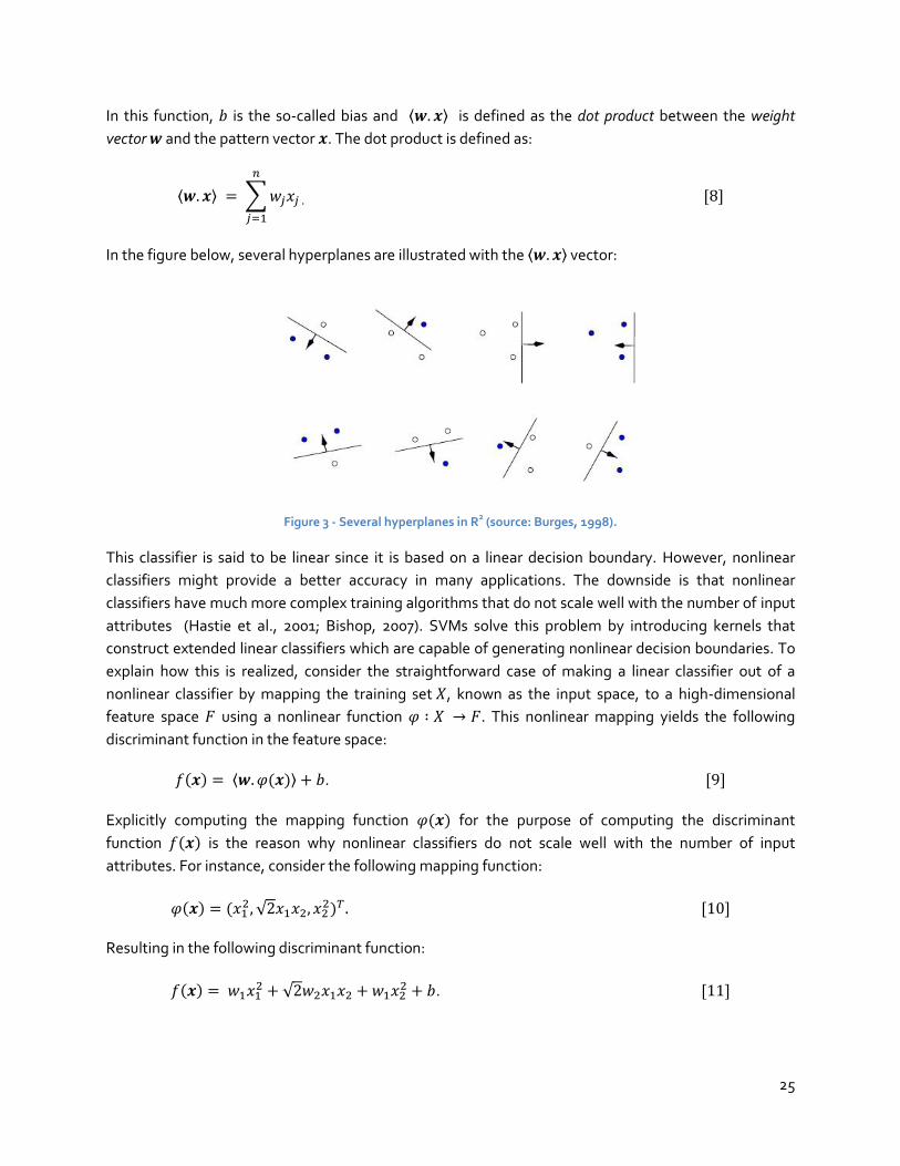
In the figure below, several hyperplanes are illustrated with the ⟨ ⟩ vector:

Figure 3 - Several hyperplanes in R2 (source: Burges, 1998).

This classifier is said to be linear since it is based on a linear decision boundary. However, nonlinear

classifiers might provide a better accuracy in many applications. The downside is that nonlinear

classifiers have much more complex training algorithms that do not scale well with the number of input

attributes (Hastie et al., 2001; Bishop, 2007). SVMs solve this problem by introducing kernels that

construct extended linear classifiers which are capable of generating nonlinear decision boundaries. To

explain how this is realized, consider the straightforward case of making a linear classifier out of a

nonlinear classifier by mapping the training set , known as the input space, to a high-dimensional

feature space using a nonlinear function . This nonlinear mapping yields the following

discriminant function in the feature space:

⟨ ⟩ . [9]

Explicitly computing the mapping function for the purpose of computing the discriminant

function is the reason why nonlinear classifiers do not scale well with the number of input

attributes. For instance, consider the following mapping function:

√

[10]

Resulting in the following discriminant function:

√

. [11]

26

As a consequence, the dimensionality of the feature space is quadratic in the dimensionality of the

input space , which results in a quadratic increase in time required to compute this discriminant

function plus a quadratic increase in memory usage for storing the attributes of the patterns. Quadratic

complexity is absolutely not feasible when one has to deal with an already large dimension in the input

space. A solution is therefore to compute the discriminant function without having to implicitly

understand the mapping function . In order to accomplish this, the weight vector must first be

expressed as a linear combination of the training instances, by:

∑

Subsequently, the discriminant function in the input space becomes:

∑ ⟨ ⟩

And the discriminant function in the feature space is therefore:

∑ ⟨ ⟩

This representation of the discriminant function in the input space and in the feature space in terms of

the variables is defined as the dual representation. The dot product ⟨ ⟩ for is

known as the kernel function, denoted by:

⟨ ⟩. [15]

If this kernel function can be computed directly as a function of the original input instances, it becomes

possible to compute the discriminant function without knowing the underlying mapping function. An

important consequence of the dual representation and the kernel function is thus that the dimension of

the feature space does not need to affect the computation complexity. The earlier mapping

√

needed to compute ⟨ ⟩ can now be replaced by ⟨ ⟩ in

which:

⟨ ⟩ √

√

,

,

⟨ ⟩ [16]

27

This has shown that the kernel can be computed without the need to explicitly compute the mapping

function . A more general form of this kernel is given as the -degree polynomial kernel and the

linear kernel for as:

⟨ ⟩ [17]

⟨ ⟩ [18]

The two figures below illustrate a 3 degree Polynomial kernel.

Figure 4 - Degree 3 polynomial kernel. The background color shows the shape of the decision surface.

Other widely used kernels are the radial basis function (RBF) kernel, also known as the gaussian kernel,

and the sigmoid kernel:

‖ ‖ [19]

[20]

The discriminant function in the feature space is now defined as:

∑

Suppose this discriminant function defines a certain hyperplane that linearly separates the training set

between the positive and negative classes. The closest vectors to this hyperplane among the vectors

in are denoted by and for the positive and negative classes respectively. The geometric margin

of the hyperplane with respect to the training set is then defined as:

28

⟨ ̂ ⟩ [22]

The vector ̂ is the unit vector in the direction of , i.e. ‖ ̂‖ . Furthermore, it is assumed

that and are equidistant from the hyperplane, which means that for an arbitrary constant ,

the following holds:

⟨ ⟩ . [23]

⟨ ⟩ [24]

Fixing the value of the discriminant function at and , setting in the above equations, adding

them together, and dividing by ‖ ‖, yields the following definition for the geometric margin:

‖ ‖ [25]

This geometric margin is illustrated in the figure below, with the closest vectors to the hyperplane

being circled:

Figure 5 - Linear separating hyperplane with the geometric margin (source: Burges, 1998).

The maximum margin classifier that linearly separates the training set between the positive and

negative classes, is that one with a discriminant function that maximizes this geometric margin. This is

equivalent to minimizing ‖ ‖ or minimizing

‖ ‖ . Finding that specific discriminant function that

maximizes the geometric margin is now equivalent to solving the following constrained optimization

problem:

‖ ‖ ,

⟨ ⟩ . [26]

29

The above optimization assumes that the training set is linearly separable, for which the constraint

⟨ ⟩ ensures that this specific discriminant function can classify each instance

correctly. However, does not necessarily need to be linearly separable. Therefore, the above

constraint needs to be adjusted so that it will allow the classifier to misclassify some instances. Even for

a linearly separable data set, this might lead to a greater margin that eventually is better than the

margin that have correctly separated all the instances. By introducing a so-called slack variable in the

constraint, a margin error or misclassification is now allowed by:

‖ ‖

⟨ ⟩ . [27]

A particular instance is misclassified if ⟨ ⟩ . Hence, If, is the case in the above

constraint, then in is misclassified. If , then in is to be within the margin, also

known as a margin error. is correctly classified if , therefore, the sum of the slack variables for

all the instances represents a bound on the number of misclassified examples, defined as the amount of

slack:

∑

{( )}

. [29]

To set an importance for minimizing the amount of slack relative to maximizing the margin, i.e. to

prioritize penalization of misclassification and margin errors, a constant multiplies the amount of

slack, also known as the soft-margin constant. The following constrained optimization problem with

the amount of slack accounted for was introduced by Cortes and Vapnik in 1995 and is known as the

soft-margin SVM:

‖ ‖ ∑

⟨ ⟩ [30]

30

The amount of slack is illustrated in the figure below:

Figure 6 - Linear separating hyperplane with the amount of slack accounted for (source: Burges, 1998).

The dual formulation of this SVM using the method of Langrage multipliers (Cortes and Vapnik, 1995;

Shölkopf and Smola, 2002; Christianini and Shawe-Taylor, 2000), as expressed in terms of variables

is defined as:

∑

∑∑

⟨ ⟩

∑

The dot product ⟨ ⟩ in the above equation is then replaced with one of the kernel functions that

were presented earlier, to perform a nonlinear transformation and a large margin separation in the

high-dimensional feature space of the kernel as has been explained before.

Due to this specific dual formulation, resulted by the use of the Lagrangian theory, the solution that is

found by the optimization problem has certain interesting properties. It has been proven that the

obtained solution is always global, since the problem formulation is convex (Burges, C.J.C., 1998). In

addition, given the fact that the discriminant function is strictly convex, it follows that the obtained

solution is also unique. These properties make overfitting unlikely to occur with the SVM. Over fitting

may however be caused by too much flexibility in the decision boundary. Nevertheless, the hyperplane

is relatively stable and gives little flexibility (Frank, 2000).

Another interesting property is that not all training vectors contribute to the obtained solution. To

explain this, consider the weight vector in terms of the vectors in the training set denoted in the dual

formulation, which is defined as:

31

∑

All the vectors for which are vectors that are either on the margin or within the margin. These

vectors are the so-called support vectors. The vectors for which , are not used to formulate the

solution. As a consequence, if these vectors that are not support vectors would have been removed

prior to the training, the exact same solution would have been obtained. This phenomenon is referred

to as the ‘sparseness’ of the SVM. This also explains that many support vectors do not necessarily result

in it overfitted solution (Thissen et al., 2003). However, the smaller the fraction of support vectors, the

less computations are required to conduct predictions on a new data set. Furthermore, the fraction of

vectors within the training set serving as support vectors is an upper bound on the error rate of the

SVM (Shölkopf and Smola, 2002). This upper bound is therefore also dependent on the constant ,

since .

3.2.2 The Theory of Support Vector Machines: Regression

The principle of the SVMs explained to this point has been for classification purposes. However, SVMs

can easily be extended to the task of regression and time series prediction, for which the focus of this

research lies on. The constrained optimization problem is now transformed to minimizing a certain cost

function as a function of the soft-margin constant . This cost function has at most deviation, also

known as the tube size of the SVM, from the actual values for all . The cost function is defined as:

‖ ‖

∑

{

| | |

|

The vector is the predicted outcome for the desired outcome . If the absolute difference between

the predicted outcome and the desired outcome is equal or larger than , measured by the ε-insensitive

loss function , the penalty function

∑

, also known as the empirical risk,

increases and penalizes that error by the amount of the soft-margin constant . Introducing the slack

variables and , that denote errors larger than +ε and –ε respectively, the constrained optimization

problem is now defined as:

‖ ‖ ∑

32

⟨ ⟩ ,

⟨ ⟩ ,

[35]

For the above optimization problem, the most recent observation is for and the earliest

observation is for . By applying Lagrangian theory to obtain the dual formulation for this

optimization problem, the weight vector equals the combination of the training data in the following

form:

∑

In this equation, and are Lagrange multipliers are associated with a specific instance . The

asterisks denote difference above and below the regression line. They satisfy the equalities:

. [37]

. [38]

Substituting this weight vector in the above equation for the regression function ⟨ ⟩ ,

yields the following discriminant function:

∑ ⟨ ⟩

To obtain the Lagrange multipliers and , the previous optimization problem has to be solved in

the dual formulation:

∑

∑

∑∑

⟨ ⟩

∑

. [40]

The vectors for which are called the support vectors. The vectors with |

| lie

outside the boundary of the discrimination function and are known as the error support vectors. The

vectors With | | lie exactly on the boundary of the discrimination function and are

33

known as the non-error support vectors. The dot product ⟨ ⟩ In the above equation can now also be

replaced with one of the kernel functions that were presented earlier.

3.2.3 Application of Support Vector Machines

SVMs have been used in many pattern recognition cases. For instance, they have been used for

handwriting recognition (Cortes and Vapnik, 1995; Schölkopf, Burges and Vapnik, 1995; Schölkopf,

Burges and Schölkopf, 1997), for object recognition (Blanz hyperplain al. 1996), for speech recognition

(Schmidt, 1996), and for face recognition (Osuna, Freund and Girosi, 1997a). With the recent

introduction of the insensitive loss function by Vapnik, SVMs were extended to solve nonlinear

regression estimation problems and have afterwards been successfully used to solve forecasting

problems in various fields. They have been benchmarked and compared on time series prediction tests,

in which their generalization performance was found to be significantly better than that of the

competing methods compared. (Müller et al., 1997, Mukherjee, Osuna and Girosi, 1997). SVMs have

been used for financial forecasting by Huang (2008), Liu and Wang (2007), Kim (2002), and Tay and Cao

(2000).

3.3 Conclusions

This chapter explored two specific computational intelligence techniques applicable to exchange rate

prediction, namely the ANN and the SVM. It has been shown that an important feature of these models

is their ability to generalize through nonlinear approximation and interpolation in usually high-

dimensional spaces (Kecman, 2001). Generalization refers to the capacity of the model to provide

correct outputs when using data that were not seen during training. This feature is extremely useful in

financial forecasting, since the underlying relationships of the financial market is often unknown or hard

to describe (Zhang, Patuwo, Hu, 1998). However, one problem with these models is that the underlying

laws governing the system to be modeled, and from which the data is generated, in this case the

exchange market, is not always clear.

It has been explained that an MLP is composed of several layers containing nodes that are

interconnected to allow the neurons to signal each other as information is processed. Each connection

between the neurons is assigned a certain weight, that determines the output of the neural network

through a nonlinear activation function. To assign certain values to these connection weights suitable

for a specific problem, the neural network needs to undergo a training process, which fall into the

categories of supervised, unsupervised, and various hybrid approaches. This research employs a

supervised training which is accomplished by feeding the neural network a set of input patterns while

attaching desired responses to those patterns, for which these desired responses are available

throughout the training. An important feature of ANNs, is that they are considered to be universal

functional approximators, thus being able to approximate any continuous function to any desired

accuracy (Irie and Miyake, 1988; Hornik et al., 1989; Cybenko, 1989; Funahashi, 1989; Hornik, 1991,

34

1993). Problems with ANNs is their excessive training times, the danger of underfitting and overfitting,

and that they require a selection of a large number of controlling parameters, for which there is no

structured way or method to obtain the most optimal parameters for a given task (Huang et al.,2004).

A basic understanding in the crucial elements of the SVM was provided, with introduced concepts as

the decision boundary, the hyperplane, the discriminant function, the geometric margin, the amount of

slack, the error function, the dual representation, and the kernel function. The basic idea of the SVM is

finding a maximum margin classifier that separates a training set between positive and negative

classes, based on a discriminant function that maximizes the geometric margin. Finding that specific

discriminant function that maximizes the geometric margin is shown to be equivalent to solving a

constrained optimization problem. The dual formulation of the SVM using the method of Langrage

multipliers (Cortes and Vapnik, 1995; Shölkopf and Smola, 2002; Christianini and Shawe-Taylor, 2000),

makes it possible to perform a nonlinear transformation and a large margin separation in the high-

dimensional feature space. An important consequence of the dual representation and the kernel

function is that the dimension of the feature space does not need to affect the computation

complexity. In addition, the solution that is found by the optimization problem has certain interesting

properties. It has been proven that the obtained solution is always global, since the problem

formulation is convex (Burges, C.J.C., 1998). Furthermore, given the fact that the discriminant function

is strictly convex, it follows that the obtained solution is also unique.

35

36

4 Design of the Prediction Models

This chapter describes the design of the SVM and the ANN for the purpose of exchange rate

prediction. The design starts with the input selection, in which the processing steps to prepare the raw

data to a suitable input for the models are given. Following is the output selection, that determines the

output of the prediction models and how this output is interpreted. Afterwards, the dependence of the

bias and variance upon certain design parameters in the SVM and the ANN model selection is

explained. Subsequently, the model selection for the SVM and the ANN is described.

4.1 Input Selection

In this research, only one data source is used, rather than using multiple sources that have a cross-

sectional relationship. By using multiple sources, microeconomic variables could be taken into account

next to the exchange rate. However, this is out of the scope of this research and has been avoided due

to complexity problems. In addition, most neural network designs for the purpose of exchange rate

prediction use only one data source (Huang et al., 2004).

Presenting the prediction models with raw financial data without any further processing is well

possible, considering the black box nature of both the SVM and the ANN. However, by properly

preparing the data, one can often attain an increase in the prediction performance and in the learning

speed (Kaastra and Boyd, 1995). The aim of this section is to investigate how to prepare and process the

financial data derived from the currency market. In doing so, the processing of the raw financial data is

broken down into five steps. These steps are (Huang et al., 2004):

1. Sampling

2. Transforming

3. Normalizing

4. Dividing

5. Windowing

For each step, it is investigated what the possible choices are, based on a literature review, and what

specific processing is chosen for in this research. A visual representation on the EUR/USD data set is

presented after certain processing steps, to illustrate that particular processing step.

37

4.1.1 Sampling

Sampling the data is a process in which two choices have to be made. The first choice is regarding the

sampling size, while the second choice is regarding the sampling rate. The sampling size is an important

factor in the forecasting ability of the prediction models. The tendency in current literature regarding

the training of ANNs and SVMs in the domain of financial forecasting is to use the largest data set

possible (Huang et al., 2004). For instance, Zhang and Hu (1998) showed that a large sample (887 data

points) out preformed a smaller sample (261 data points) in the training of an ANN for the purpose of

exchange rate prediction.

However, Kang (1991) argues that neural network models for the purpose of time series forecasting do

not necessarily require a large data set to perform well. In fact, many different sizes of data sets have

been used by neural network researchers, ranging from one year to 16 years (Jamal and Sundar, 1998;

Refenes, 2000; Tenti, 1996; Walczak et al., 1998; Zhang and Hu, 1998). Walczak (2001) have trained

ANNs with different sizes of training sample sets for the purpose of exchange rate prediction. He

concludes that two years of training data at a daily sampling rate is usually all that is required to acquire

the most optimal forecasting accuracy.

A total different approach in determining the optimal data set size for the purpose of exchange rate

prediction is given by Huang et al. (2002), in which they propose to use change point detection. They

argue that the behavior of exchange rates is continuously evolving over time and that certain change

points can be identified which divide data into several homogeneous groups that take heterogeneous

characteristics from each other. The problem however is that there is no general approach to identify

these change points and it will therefore be subjected to the researcher’s interpretation.

The sampling rate defines at what rate the raw data is sampled in terms of time. Sampling every data

point in the raw data set is equivalent to using all the data that is available in the data set, ensuring that

there is no information loss. The raw data is very high frequent, representing every event change in the

price, resulting in an extremely large data set for a relatively small time window. Accumulated over the

period of approximately 6 1/2 years, the data consists of exactly 63413970 data points, well over 60

million. In some cases, the price could have changed three to four times within the second. Not only

does this provide a huge data set even within a single day making it a very time-consuming process to

analyze, but the input window for the SVM has to be incredible large as well to preserve an overview of

the daily movements. For these reasons, it is desired to sample the data at a less frequent rate.

A few options for the sampling rate are sampling every minute, every hour, twice a day, every day,

every week, twice a month, every month, every year. Most researchers who have studied the

application of ANNs and SVMs in financial forecasting, have used the daily closing price as the sampling

rate for their data (Francis and Cao, 2001; Kim, 2002; Liu and Wang, 2008; Tay and Cao, 2002; Huang et

al., 2004). An average over a specified time of a specific sampling rate is also sometimes used, in the

form of a moving average indicator as input to the prediction model (Dunis, 2008).

In this research, the maximum sample size is 6 1/2 years, constrained by the used EUR/USD data set.

Given this sample size, any sampling rate higher than a week is not practical, since the prediction model

38

will have to little data points to train on. Applying a daily sampling rate on this EUR/USD data set

provides roughly 1500 data points. The daily sampling rate is preferred since, as already mentioned, it is

the most popular sampling rate in financial forecasting. Considering the literature mentioned above, a

sample size of 1500 data points is certainly reasonable, and it is not necessarily required to use a larger

data set in achieving a higher prediction performance.

The figure below gives an overview of the daily closing price over the EUR/USD data set, sampled at 6

AM (chosen arbitrary since there is no official opening or closing time for a trading day in the currency

market) for each day:

In reviewing the figure above, one may notice that each time component may be composed of a

structural component and a noise component. The ratio between the structural component and a time

component is difficult to assess. However, it may well be that the sampling rate with a higher frequency

would yield a higher complexity of the structural component. As a consequence, different sampling

rates may yield very different patterns, containing information in different specific ways. Therefore, in

this chapter, regression models with different sampling rates will be compared with each other on the

prediction performance. The sampling rates to be compared are the daily and hourly sampling rates,

with the sampling size of 1500 data points for each sampling rate.

1,15

1,20

1,25

1,30

1,35

1,40

1,45

1,50

1,55

1,60

1,65

1

59

11

7

17

5

23

3

29

1

34

9

40

7

46

5

52

3

58

1

63

9

69

7

75

5

81

3

87

1

92

9

98

7

10

45

11

03

11

61

12

19

12

77

13

35

13

93

14

51

15

09

Qu

ote

t

EUR/USD - Daily closing price 2004-2009 EUR/USD

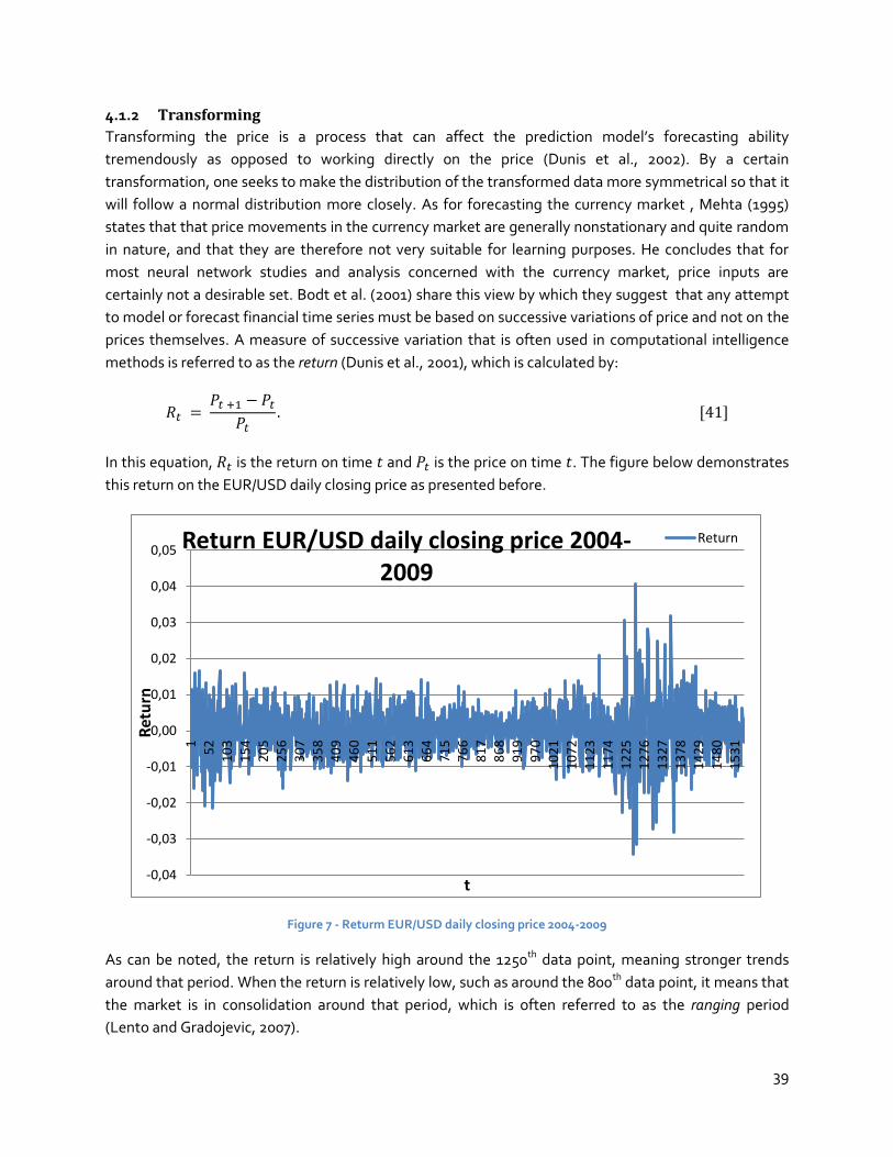
39

4.1.2 Transforming

Transforming the price is a process that can affect the prediction model’s forecasting ability

tremendously as opposed to working directly on the price (Dunis et al., 2002). By a certain

transformation, one seeks to make the distribution of the transformed data more symmetrical so that it

will follow a normal distribution more closely. As for forecasting the currency market , Mehta (1995)

states that that price movements in the currency market are generally nonstationary and quite random

in nature, and that they are therefore not very suitable for learning purposes. He concludes that for

most neural network studies and analysis concerned with the currency market, price inputs are

certainly not a desirable set. Bodt et al. (2001) share this view by which they suggest that any attempt

to model or forecast financial time series must be based on successive variations of price and not on the

prices themselves. A measure of successive variation that is often used in computational intelligence

methods is referred to as the return (Dunis et al., 2001), which is calculated by:

In this equation, is the return on time and is the price on time . The figure below demonstrates

this return on the EUR/USD daily closing price as presented before.

Figure 7 - Returm EUR/USD daily closing price 2004-2009

As can be noted, the return is relatively high around the 1250th data point, meaning stronger trends

around that period. When the return is relatively low, such as around the 800th data point, it means that

the market is in consolidation around that period, which is often referred to as the ranging period

(Lento and Gradojevic, 2007).

-0,04

-0,03

-0,02

-0,01

0,00

0,01

0,02

0,03

0,04

0,05

15

21

03

15

42

05

25

63

07

35

84

09

46

05

11

56

26

13

66

47

15

76

68

17

86

89

19

97

01

02

11

07

21

12

31

17

41

22

51

27

61

32

71

37

81

42

91

48

01

53

1

Ret

urn

t

Return EUR/USD daily closing price 2004-2009

Return

40

Dunis and Williams (2002) showed that by transforming the data into returns, the time series will

become stationary which is a useful statistical property. They performed ADF and Philips-Peron tests

statistics on EUR/USD return series which provided a formal confirmation that this transformation

returns a stationary series at the 5% significance level. However, they do note that transforming the

price into returns often creates noisy time series.

Some researchers follow a very different approach, such as Kim (2003), as he suggests to use technical

indicators (as the ones described before) as input for the prediction model. Kim (2003) used 12 different

technical indicators, such as the stochastic technical indicator, the momentum, and the relative

strength Index. The advantage is that the price will be smoothed out. However , thereby one is actually

combining different models, increasing the complexity of the total system. In this research, the price

will be transformed to returns as explained before.

4.1.3 Normalizing

Normalization is the process of transforming the input data into an appropriate form for the prediction

models. Several studies on the effects of data normalization, most specifically focused on ANNs, show

different results and opinions whether there is a need to normalize the data set.

Shankar et al. (1996) argue that for the purpose of general classification problems which are solved by

ANNs and SVMs, normalizing the input data provides a lower mean square error. This effect becomes

stronger as the sample size becomes smaller. Engelbrecht et al. (1994) have shown similar results.

However, El Shazly et al. (1997) have found that data normalization does not necessarily lead to better

forecasting performance in classification problems. Zhang et Hu (1998) did not normalize their data for

the purpose of exchange rate prediction, since they believe that there is no significant difference

between normalized and original data, based on their experience. Nevertheless, many researchers in

this field normalized the input data and they advise this to avoid computational problems, to meet

algorithm requirements, and to facilitate the learning process (Lapedis and Farber, 1988; Sharda and

Patil, 1992; Srinivasan et al., 1994).

One advantage of normalizing is that it ensures that input attributes with a larger value do not

overwhelm input attributes with a smaller value, which in turn will reduce the prediction error. In some

cases, normalizing the input data is absolutely necessary if a function is valid only for a limited range.

For instance, an ANN that uses the sigmoid function (0.0 -1.0) can only generate output values inside

this range. Consequently, in training this neural network, the output that corresponds to the training

input should therefore be normalized to this range.

Azoff (1994) proposes four methods for general input normalization which are along channel

normalization, across channel normalization, mixed channel normalization, and external normalization.

Choosing one of these mentioned methods will depend on the composition of the desired input vector.

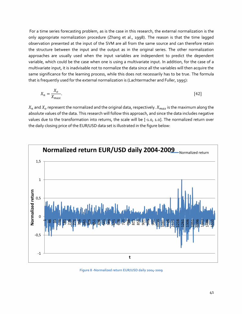
41

For a time series forecasting problem, as is the case in this research, the external normalization is the

only appropriate normalization procedure (Zhang et al., 1998). The reason is that the time lagged

observation presented at the input of the SVM are all from the same source and can therefore retain

the structure between the input and the output as in the original series. The other normalization

approaches are usually used when the input variables are independent to predict the dependent

variable, which could be the case when one is using a multivariate input. In addition, for the case of a

multivariate input, it is inadvisable not to normalize the data since all the variables will then acquire the

same significance for the learning process, while this does not necessarily has to be true. The formula

that is frequently used for the external normalization is (Lachtermacher and Fuller, 1995):

and represent the normalized and the original data, respectively. is the maximum along the

absolute values of the data. This research will follow this approach, and since the data includes negative

values due to the transformation into returns, the scale will be [-1.0, 1.0]. The normalized return over

the daily closing price of the EUR/USD data set is illustrated in the figure below:

Figure 8 -Normalized return EUR/USD daily 2004-2009

-1

-0,5

0

0,5

1

1,5

14

69

11

36

18

1

22

62

71

31

63

61

40

6

45

14

96

54

15

86

63

1

67

67

21

76

68

11

85

6

90

19

46

99

11

03

61

08

1

11

26

11

71

12

16

12

61

13

06

13

51

13

96

14

41

14

86

15

31

No

rmal

ized

ret

urn

t

Normalized return EUR/USD daily 2004-2009 Normalized return

42

4.1.4 Dividing

Dividing the data in several subsets by appointing specific data for training purposes and for test

purposes, is required for building an SVM and an ANN. Usually, the data is divided into three subsets,

one set for training, one set for testing, and one set for validating. The training set is used for

developing the SVM, the test set is used to evaluate the forecasting ability of the SVM. The validation

set is usually part of the test set and is used to avoid the over fitting problem or to determine the

stopping point of the training process (Weigend et al., 1992).

There is no general solution or approach in dividing the data in appropriate sizes into a training and test

set. However, there are several factors that should be considered in making the decision, most notably

the problem characteristics, the data type, and the size of the available data (Zhang et al., 1998). For

time series forecasting problems, as is the case in this research, it is absolutely critical to have both the

training and test sets to be representative of the underlying mechanism, which has implications on the

size of these sets. Yao et al. (2000) suggests that the training set should contain 70% of the data, the

validation set 20%, and the tests and 10%, based on the authors' experience. Other researchers have

used 80% for the training data, or even 90%, while not touching on the reasons for it (Huang et al.,

2004). Granger (1993) suggest that at least 20% should be appointed to the testing data for nonlinear

forecasting models. Tay and Cao (2001) and Kim (2003) have both used 80% for the training set and

20% for the validation and test set in applying SVMs for financial time series forecasting. This research

use the following percentages, i.e. 70% will be used for training, and 30% will be used for validation

(20%) and testing (10%).

4.1.5 Windowing

Windowing the data concerns selecting the number of samples that form successive inputs to the

model, by which the subsequent value will be predicted. For instance, if the window size is chosen to be

3, then ̂ is the predicted output with the input being exactly 3 number of successive samples, i.e. ,

, and . If the window size is chosen to be 10, then ̂ is predicted by to In addition,

the inputs in the window may be weighted to emphasize certain input samples above other samples.

For instance, an exponential weighted window of 3 would weigh the inputs with ,

,

.

That way, the assumption is that the last input , contains more information regarding what the

upcoming value will be compared to .

Regression models with different window sizes will be compared to each other on the prediction

performance to find an appropriate window size. Windows with , , and will be

chosen. This is a matter of choice, justified by the intuitive feeling that a lower window size is not

sufficient to capture a pattern while a larger window size would yield a too sophisticated structured

pattern.

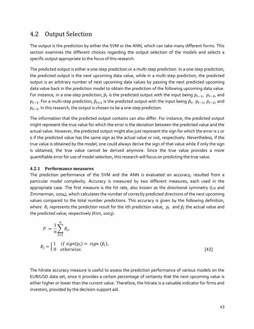
43

4.2 Output Selection

The output is the prediction by either the SVM or the ANN, which can take many different forms. This

section examines the different choices regarding the output selection of the models and selects a

specific output appropriate to the focus of this research.

The predicted output is either a one-step prediction or a multi-step prediction. In a one-step prediction,

the predicted output is the next upcoming data value, while in a multi-step prediction, the predicted

output is an arbitrary number of next upcoming data values by passing the next predicted upcoming

data value back in the prediction model to obtain the prediction of the following upcoming data value.

For instance, in a one-step prediction, ̂ is the predicted output with the input being , , and

. For a multi-step prediction, ̂ is the predicted output with the input being ̂ , , and

. In this research, the output is chosen to be a one-step prediction.

The information that the predicted output contains can also differ. For instance, the predicted output

might represent the true value for which the error is the deviation between the predicted value and the

actual value. However, the predicted output might also just represent the sign for which the error is 1 or

0 if the predicted value has the same sign as the actual value or not, respectively. Nevertheless, if the

true value is obtained by the model, one could always derive the sign of that value while if only the sign

is obtained, the true value cannot be derived anymore. Since the true value provides a more

quantifiable error for use of model selection, this research will focus on predicting the true value.

4.2.1 Performance measures

The prediction performance of the SVM and the ANN is evaluated on accuracy, resulted from a

particular model complexity. Accuracy is measured by two different measures, each used in the

appropriate case. The first measure is the hit rate, also known as the directional symmetry (Lu and

Zimmerman, 2004), which calculates the number of correctly predicted directions of the next upcoming

values compared to the total number predictions. This accuracy is given by the following definition,

where represents the prediction result for the th prediction value, and ̂ the actual value and

the predicted value, respectively (Kim, 2003):

∑

{ ̂

The hitrate accuracy measure is useful to assess the prediction performance of various models on the

EUR/USD data set, since it provides a certain percentage of certainty that the next upcoming value is

either higher or lower than the current value. Therefore, the hitrate is a valuable indicator for firms and

investors, provided by the decision-support aid.

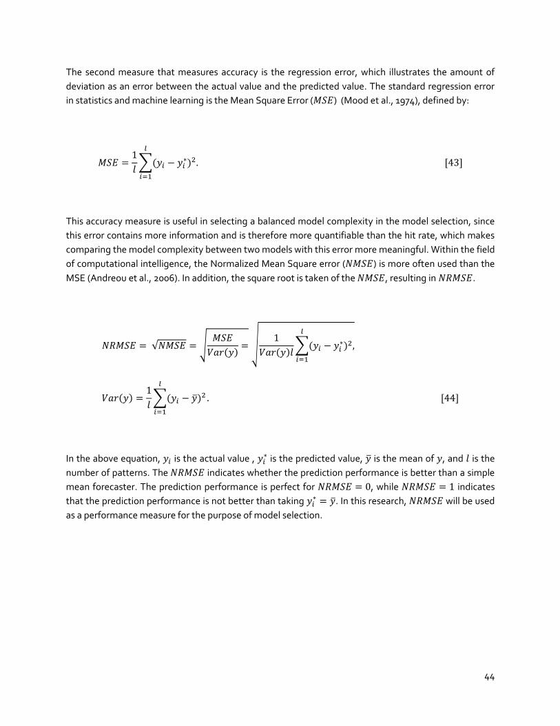
44

The second measure that measures accuracy is the regression error, which illustrates the amount of

deviation as an error between the actual value and the predicted value. The standard regression error

in statistics and machine learning is the Mean Square Error ( ) (Mood et al., 1974), defined by:

∑

This accuracy measure is useful in selecting a balanced model complexity in the model selection, since

this error contains more information and is therefore more quantifiable than the hit rate, which makes

comparing the model complexity between two models with this error more meaningful. Within the field

of computational intelligence, the Normalized Mean Square error ( ) is more often used than the

MSE (Andreou et al., 2006). In addition, the square root is taken of the , resulting in .

√ √

√

∑

∑ ̅

In the above equation, is the actual value , is the predicted value, ̅ is the mean of , and is the

number of patterns. The indicates whether the prediction performance is better than a simple

mean forecaster. The prediction performance is perfect for , while indicates

that the prediction performance is not better than taking ̅. In this research, will be used

as a performance measure for the purpose of model selection.

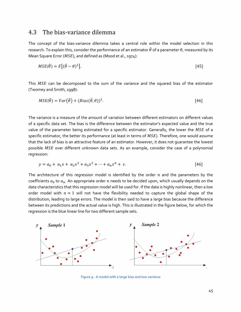
45

4.3 The bias-variance dilemma

The concept of the bias-variance dilemma takes a central role within the model selection in this

research. To explain this, consider the performance of an estimator ̂ of a parameter , measured by its

Mean Square Error ( ), and defined as (Mood et al., 1974):

( ̂ [ ̂ ] [45]

This can be decomposed to the sum of the variance and the squared bias of the estimator

(Twomey and Smith, 1998):

( ̂ ( ̂) ̂ [46]

The variance is a measure of the amount of variation between different estimators on different values

of a specific data set. The bias is the difference between the estimator’s expected value and the true

value of the parameter being estimated for a specific estimator. Generally, the lower the of a

specific estimator, the better its performance (at least in terms of ). Therefore, one would assume

that the lack of bias is an attractive feature of an estimator. However, it does not guarantee the lowest

possible over different unknown data sets. As an example, consider the case of a polynomial

regression:

The architecture of this regression model is identified by the order and the parameters by the

coefficients to . An appropriate order needs to be decided upon, which usually depends on the

data characteristics that this regression model will be used for. If the data is highly nonlinear, then a low

order model with will not have the flexibility needed to capture the global shape of the

distribution, leading to large errors. The model is then said to have a large bias because the difference

between its predictions and the actual value is high. This is illustrated in the figure below, for which the

regression is the blue linear line for two different sample sets.

Figure 9 - A model with a large bias and low variance

46

On the other hand, the variance in this model is low, which is illustrated in the figure above given that

the blue regression line did not change much for the both sample sets. If the order of the model is

increased to account for this low variance, making the model more complex, then the regression line

will fit the data better but it will also make it very sensitive to the details of the data. A different data set

would lead to a completely different model, with completely different predictions. The model is then

said to have a large variance because the variance, i.e. the difference between the estimators is large.

This is illustrated in the figure below:

Figure 10 - A model with a small bias and a high variance

In other words, a low order regression model has a high bias on the estimated values (causing large

errors) but a low variance between different estimators, while a high order regression model has a low

bias on the estimated values but a high variance between different estimators (causing large errors).

This is the essence of the bias-variance dilemma, also known as the bias-variance tradeoff. A too low

model complexity will underfit the training data while a too high model complexity will overfit the

training data. A good model should balance the bias and variance, trying to keep each as low as

possible. The general relation between the bias and variance to the model complexity can be stated as

follows.

The bias of the model decreases with the model complexity, since the added degrees of freedom makes it easier to fit to the actual relationship.

The variance of the model increases with the model complexity, since the added degrees of freedom increases the risk to fit to noise.

Selecting the appropriate model complexity for both the ANN and the SVM which will be based upon

the above two notions. Lastly, it is worth mentioning that a prediction model with a high model

complexity is said to be overfitted by the training set, whereas a prediction model with a low model

complexity is said to be underfitted by the training set.

47

4.4 The SVM model selection

This section explores the appropriate SVM parameters for the purpose of exchange rate regression and

aims to identify a suitable range for these parameters that yields a balanced SVM in terms of model

complexity. The parameters are the tube size , the soft-margin constant , and a certain kernel

.

4.4.1 The SVM architecture

As has been shown before, the extension of the hard-margin SVM to the soft-margin SVM, introduced

by Cortes and Vapnik in 1995, sets an importance for minimizing the amount of slack relative to

maximizing the margin, i.e. to prioritize penalization of misclassification and margin errors. This

resulted in the following cost function, presented in the primal form to clearly understand the effects of

and :

‖ ‖

∑

{

| | |

|

The vector is the predicted outcome for the desired outcome . If the absolute difference between

the predicted outcome and the desired outcome is equal or larger than , measured by the ε-insensitive

loss function , the penalty function

∑

, also known as the empirical risk,

increases and penalizes that error by the amount of the soft-margin constant (Ben Hur and Weston,

2007). Within the context of the bias-variance dilemma, the soft-margin SVM thus allows the tuning of

the variance and the bias by tuning the soft-margin constant that defines the trade-off between

maximizing the margin and minimizing the amount of slack.

The larger , the larger the priority to penalize errors relative to maximizing the margin, the larger

increase of the penalty function, hence the smaller the bias and the higher the variance. If the amount

of slack is forced to be minimized by setting , than the maximum margin

‖ ‖ will be obtained by

minimizing

‖ ‖ . For this extreme, the SVM achieves the lowest variance and the highest bias. Vice

versa, if , the SVM achieves the highest variance and the lowest bias.

The tube size also affects the model complexity. The larger , the smaller increase of the penalty

function since fewer elements will satisfy the condition | | , hence the larger the bias and the

lower the variance. This is summarized in the following two notions:

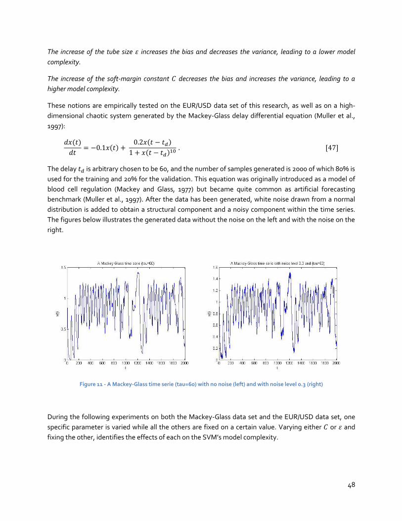
48

The increase of the tube size increases the bias and decreases the variance, leading to a lower model

complexity.

The increase of the soft-margin constant decreases the bias and increases the variance, leading to a

higher model complexity.

These notions are empirically tested on the EUR/USD data set of this research, as well as on a high-

dimensional chaotic system generated by the Mackey-Glass delay differential equation (Muller et al.,

1997):

The delay is arbitrary chosen to be 60, and the number of samples generated is 2000 of which 80% is

used for the training and 20% for the validation. This equation was originally introduced as a model of

blood cell regulation (Mackey and Glass, 1977) but became quite common as artificial forecasting

benchmark (Muller et al., 1997). After the data has been generated, white noise drawn from a normal

distribution is added to obtain a structural component and a noisy component within the time series.

The figures below illustrates the generated data without the noise on the left and with the noise on the

right.

Figure 11 - A Mackey-Glass time serie (tau=60) with no noise (left) and with noise level 0.3 (right)

During the following experiments on both the Mackey-Glass data set and the EUR/USD data set, one

specific parameter is varied while all the others are fixed on a certain value. Varying either or and

fixing the other, identifies the effects of each on the SVM’s model complexity.

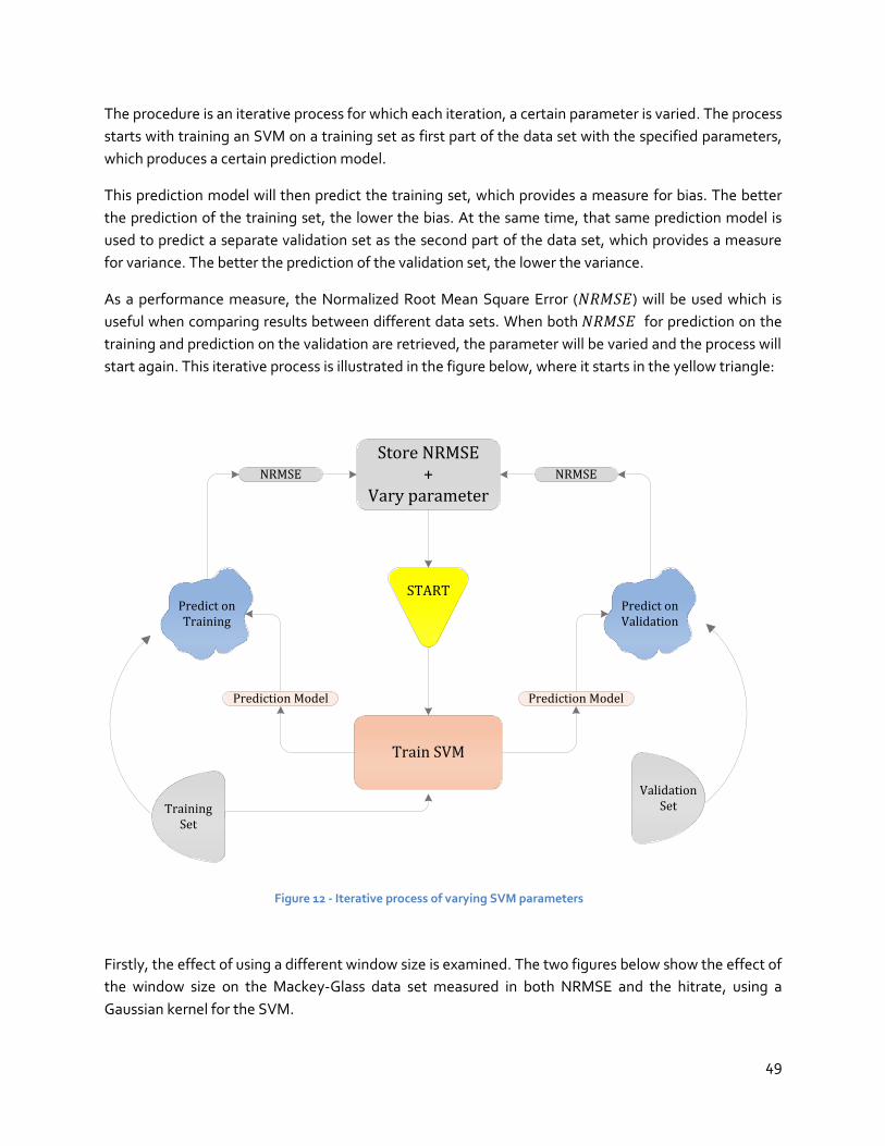
49

Validation SetTraining

Set

Predict on Training

Train SVM

Predict on Validation

START

Store NRMSE+

Vary parameter

NRMSE NRMSE

Prediction Model Prediction Model

The procedure is an iterative process for which each iteration, a certain parameter is varied. The process

starts with training an SVM on a training set as first part of the data set with the specified parameters,

which produces a certain prediction model.

This prediction model will then predict the training set, which provides a measure for bias. The better

the prediction of the training set, the lower the bias. At the same time, that same prediction model is

used to predict a separate validation set as the second part of the data set, which provides a measure

for variance. The better the prediction of the validation set, the lower the variance.

As a performance measure, the Normalized Root Mean Square Error ( ) will be used which is

useful when comparing results between different data sets. When both for prediction on the

training and prediction on the validation are retrieved, the parameter will be varied and the process will

start again. This iterative process is illustrated in the figure below, where it starts in the yellow triangle:

Firstly, the effect of using a different window size is examined. The two figures below show the effect of

the window size on the Mackey-Glass data set measured in both NRMSE and the hitrate, using a

Gaussian kernel for the SVM.

Figure 12 - Iterative process of varying SVM parameters

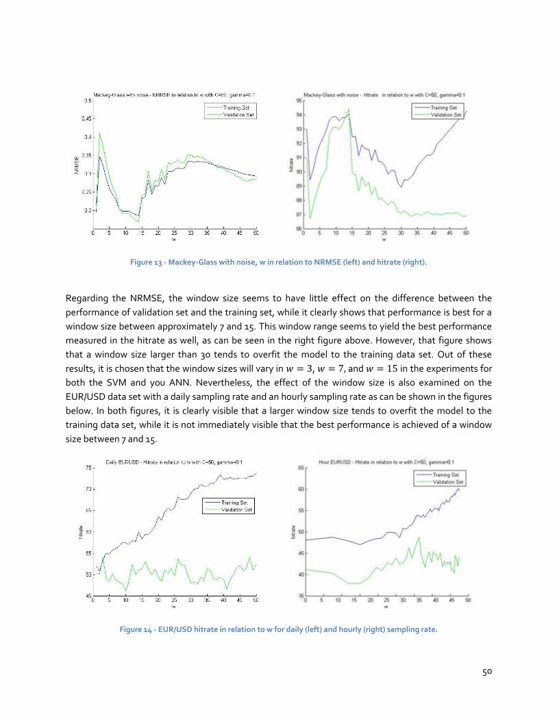
50

Figure 13 - Mackey-Glass with noise, w in relation to NRMSE (left) and hitrate (right).

Regarding the NRMSE, the window size seems to have little effect on the difference between the

performance of validation set and the training set, while it clearly shows that performance is best for a

window size between approximately 7 and 15. This window range seems to yield the best performance

measured in the hitrate as well, as can be seen in the right figure above. However, that figure shows

that a window size larger than 30 tends to overfit the model to the training data set. Out of these

results, it is chosen that the window sizes will vary in , and in the experiments for

both the SVM and you ANN. Nevertheless, the effect of the window size is also examined on the

EUR/USD data set with a daily sampling rate and an hourly sampling rate as can be shown in the figures

below. In both figures, it is clearly visible that a larger window size tends to overfit the model to the

training data set, while it is not immediately visible that the best performance is achieved of a window

size between 7 and 15.

Figure 14 - EUR/USD hitrate in relation to w for daily (left) and hourly (right) sampling rate.

51

All the following experiments in this section regarding the model selection of the SVM will be

conducted with a window size of 7 and a Gaussian kernel for the SVM.

In the figure below, the effect of the soft-margin constant on the performance of the Mackey-Glass

data set for both the NRMSE and the hitrate is illustrated, with

Figure 15 - Mackey-Glass with noise, C in relation to NRMSE (left) and hitrate (right) for SVM regression.

As can be noted, the soft-margin constant is indeed proportional to the model complexity of the

SVM. The more Increases, the better the prediction on the training set and the poorer prediction on

the validation set. In addition, the more decreases, the closer are the errors of the predictions for the

training set and a validation set to each other, resembling a low model complexity. Hence , for large

values of , the model overfits the data, while for small values of , the model underfits the data. This

finding is consistent with the earlier notion, that the constant decreases the bias and increases the

variance, leading to a higher model complexity. The figure below shows that the number of support

vectors increase as increases. The two figures below show the effect of the soft-margin constant on

the EUR/USD data set for daily and hourly sample rate.

52

Figure 16 - EUR/USD, C in relation to hitrate for daily (left) and hourly (right) sampling rate in SVM regression.

As can be seen in the above two figures, the effect of the soft-margin constant on the model

complexity with the EUR/USD data set is less clearly visible as with the Mackey-Glass data set. Between

the daily sample rate and the hourly sample rate, the effect is slightly more clear on the daily sample

rate. Furthermore, it is noticed that the overall performance of both the training set and the validation

set is worse in the hourly sampling rate compared to the daily sampling rate with varying . Based on

the results above, retrieved from experiments on the Mackey-Glass dataset as well as on the EUR/USD

dataset, an appropriate range for the soft-margin constant to be used in the experiments is between

and .

The following parameter is the tube size . Its effect on the model’s complexity is illustrated in the

figure below on the Mackey-Glass data set for both the NRMSE and the hitrate performance measure.

Figure 17 - Mackey-Glass with noise, epsilon in relation to NRMSE (left) and hitrate (right) for SVM regression.

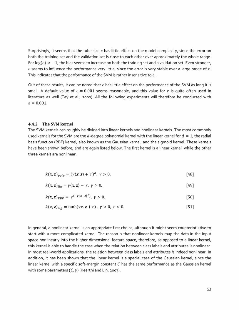
53

Surprisingly, it seems that the tube size has little effect on the model complexity, since the error on

both the training set and the validation set is close to each other over approximately the whole range.

For , the bias seems to increase on both the training set and a validation set. Even stronger,

seems to influence the performance very little, since the error is very stable over a large range of .

This indicates that the performance of the SVM is rather insensitive to .

Out of these results, it can be noted that has little effect on the performance of the SVM as long it is

small. A default value of seems reasonable, and this value for is quite often used in

literature as well (Tay et al., 2000). All the following experiments will therefore be conducted with

.

4.4.2 The SVM kernel

The SVM kernels can roughly be divided into linear kernels and nonlinear kernels. The most commonly

used kernels for the SVM are the -degree polynomial kernel with the linear kernel for , the radial

basis function (RBF) kernel, also known as the Gaussian kernel, and the sigmoid kernel. These kernels

have been shown before, and are again listed below. The first kernel is a linear kernel, while the other

three kernels are nonlinear.

⟨ ⟩ [48]

⟨ ⟩ [49]

‖ ‖ [50]

[51]

In general, a nonlinear kernel is an appropriate first choice, although it might seem counterintuitive to

start with a more complicated kernel. The reason is that nonlinear kernels map the data in the input

space nonlinearly into the higher dimensional feature space, therefore, as opposed to a linear kernel,

this kernel is able to handle the case when the relation between class labels and attributes is nonlinear.

In most real-world applications, the relation between class labels and attributes is indeed nonlinear. In

addition, it has been shown that the linear kernel is a special case of the Gaussian kernel, since the

linear kernel with a specific soft-margin constant has the same performance as the Gaussian kernel

with some parameters ) (Keerthi and Lin, 2003).

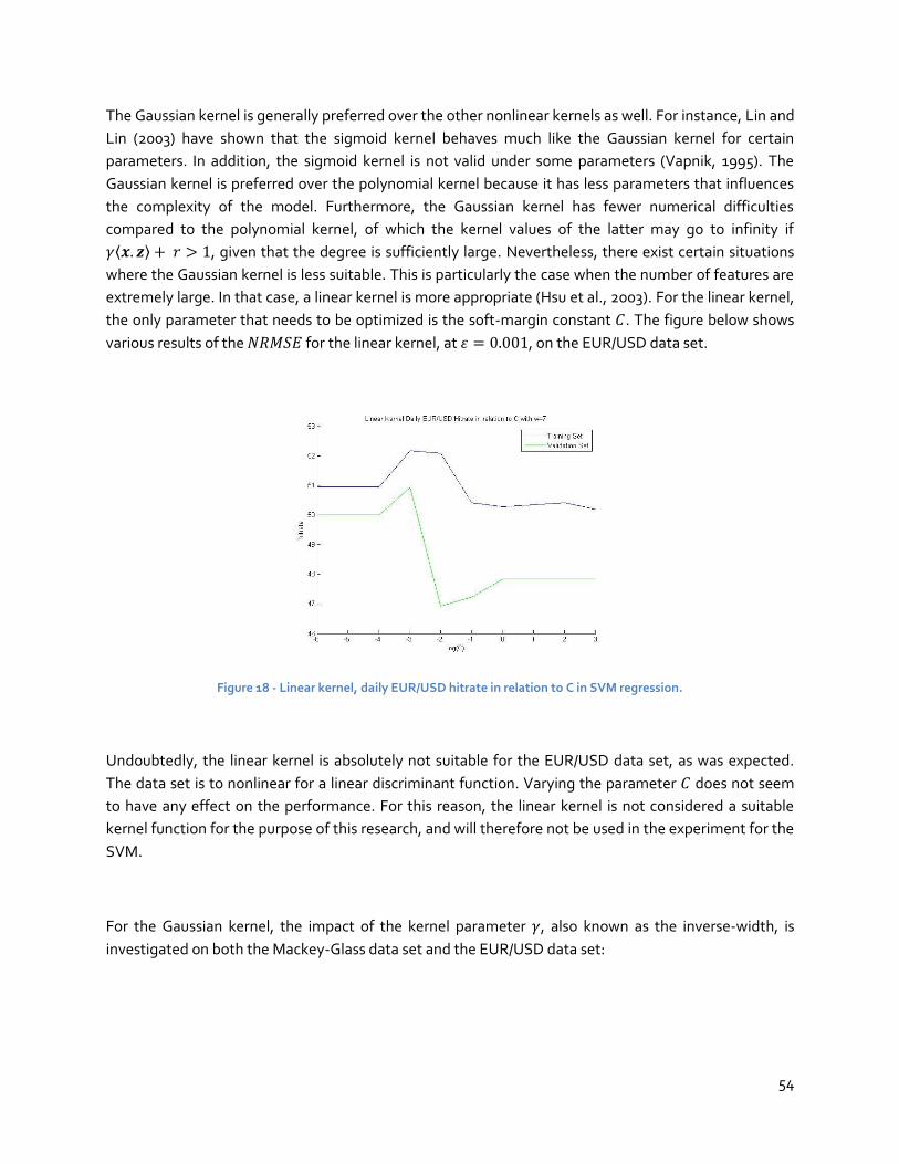
54

The Gaussian kernel is generally preferred over the other nonlinear kernels as well. For instance, Lin and

Lin (2003) have shown that the sigmoid kernel behaves much like the Gaussian kernel for certain

parameters. In addition, the sigmoid kernel is not valid under some parameters (Vapnik, 1995). The

Gaussian kernel is preferred over the polynomial kernel because it has less parameters that influences

the complexity of the model. Furthermore, the Gaussian kernel has fewer numerical difficulties

compared to the polynomial kernel, of which the kernel values of the latter may go to infinity if

⟨ ⟩ , given that the degree is sufficiently large. Nevertheless, there exist certain situations

where the Gaussian kernel is less suitable. This is particularly the case when the number of features are

extremely large. In that case, a linear kernel is more appropriate (Hsu et al., 2003). For the linear kernel,

the only parameter that needs to be optimized is the soft-margin constant . The figure below shows

various results of the for the linear kernel, at , on the EUR/USD data set.

Figure 18 - Linear kernel, daily EUR/USD hitrate in relation to C in SVM regression.

Undoubtedly, the linear kernel is absolutely not suitable for the EUR/USD data set, as was expected.

The data set is to nonlinear for a linear discriminant function. Varying the parameter does not seem

to have any effect on the performance. For this reason, the linear kernel is not considered a suitable

kernel function for the purpose of this research, and will therefore not be used in the experiment for the

SVM.

For the Gaussian kernel, the impact of the kernel parameter , also known as the inverse-width, is

investigated on both the Mackey-Glass data set and the EUR/USD data set:

55

Figure 19 - Mackey-Glass with noise, gamma in relation to NRMSE (left) and hitrate (right) in SVM regression.

Clearly, the inverse-width is related to the model complexity of the SVM. The more increases, the

better the prediction on the training set and the poorer prediction on the validation set. Thus , for large

values of , the model overfits the data, while for small values of , the model underfits the data. To

understand this, one needs to examine the role of the inverse-width parameter within the Gaussian

kernel function:

‖ ‖ . [50]

In essence, the kernel function above describes a region around a fixed vector , for which any

particular vector , the function is nonzero. This region border is defined by the distance between the

vector and any vector , denoted by ‖ ‖ , being much larger than

√ . With regard to the

discriminant function in the dual representation, as given below, this region translates into a sum of

regions for which the vector is the support vector, for all support vectors.

∑

Therefore, for small values of , any particular vector in the validation set has a nonzero kernel value

in the above kernel function relative to any support vector retrieved from the training set, resulting in

under fitting the data. On the other hand, for large values of , a particular vector in the validation set

must be located close to one of the support vectors to have a nonzero kernel value, for which this

closeness translates to overfitting the data.

The above results on the Mackey-Glass data set for various seem somewhat consistent on the

EUR/USD data set as shown in the figures below, where for large values of , the model tends to overfit

to the training data set.

56

Figure 20 - EUR/USD hitrate in relation to gamma for a daily (left) and hourly (right) sampling rate in SVM regression.

Based on the aforementioned results, an appropriate range for the inverse-width kernel parameter is

between and .

4.5 ANN Model Selection

Since the ANN in this research is merely meant as a comparison model for the SVM, a less extensive

model selection is described in this section. Most of the choices regarding the model selection of the

ANN is based on the paper by Kaastra and Boyd (1995) in “Designing a neural network for forecasting

financial and economic time series”.

As explained before, the ANN that is used in this research is in the multilayer perceptron, which is a

feedforward backpropagation neural network. The term feedforward refers to the fact that the

information flow within the neural network passes through the input layer and flows to the output

layer. The back propagation neural network is the most common multilayer neural network, used in

approximated 80% of all applications and the most widely used in financial time series forecasting as

well (Caudill, 1992).

The ANN model can be described in its neurodynamics and its architecture. The neurodynamics of the

network describe the characteristics of an individual neuron which include for instance its transfer

function (Nelson et al., 1991). The architecture of the network describes the structure of each layer and

the interconnections between these layers. It thereby describes the number of layers, the number of

neurons within each layer, and the connections between these neurons.

4.5.1 Neurodynamics of the network

The most important aspect regarding model selection of the ANN through neurodynamics is the

transfer function. The transfer function is a mathematical formula that determines the output of a

specific processing neuron, also referred to as the activation or threshold function. The purpose of this

57

function is to prevent outputs from reaching very large values that can thereby inhibit the training

process (Kaastra and Boyd, 1996). A few examples of the transfer function is the sigmoid function, the

hyperbolic tangent, and the linear function. The linear function is less appropriate within this research

since the data is of nonlinear nature. The sigmoid function and the hyperbolic tangent function are also

one of the most used transfer functions in time series prediction (Zhang et al., 1997).

[53]

( ) (

)

∑

In the above equations, denotes the real valued weights, denotes the input values, and Denotes

the number of inputs to the neurons from the previous layer (Andreou et al., 2006). The sigmoid

transfer function should be used when the neural network needs to learn average behavior, while the

hyperbolic tangent function should be used when the learning involves deviations from the average

(Klimasauskas, 1993). Since the data in this research is scaled between -1 and 1, the hyperbolic tangent

function is the only appropriate transfer function between the two since its range is between -1 and 1

while the sigmoid function’s range is between 0 and 1. In this research, the hyperbolic tangent function

will be used as the transfer function for the ANN.

4.5.2 Architecture of the network

The input layer of the neural network will contain exactly number of neurons, where defines the

window size. The output layer will contain exactly one neuron, which represents the next upcoming

value of the window, i.e. the predicted value. The number of hidden layers and the number of neurons

within these hidden layers define the model complexity of the neural network (Baum and Haussler,

1989). Given that sufficient number of hidden neurons are used, the standard back propagation neural

networ1k using an arbitrary transfer function is able to approximate any measurable function very

precisely (Hornik et al., 1989). Furthermore, it is demonstrated that a three layer back propagation

neural network is able to approximate any continuous mapping (Hecht-Nielson, 1989).

Referring to the bias-variance dilemma explained earlier, a large number of hidden layers and neurons

within these hidden layers will yield a higher model complexity with a low bias and high variance. Vice

versa, a small number of hidden layers and neurons within these hidden layers will yield a lower model

complexity with a high bias and low variance.

The increase of the number of hidden layers and the neurons within these hidden layers leads to a decrease

in the bias and an increases the variance, resulting in a higher model complexity.

58

Regarding the number of hidden layers, it is common practice within the field of financial forecasting to

use only one layer and very occasionally two layers (Kaastra and Boyd, 1996). Using one hidden layer

has shown to perform very well (Zhang et al., 1997). Furthermore, the number of neurons within these

hidden layers alone can adjust the models complexity fairly well so that the number of neurons is the

only parameter to tune with regard to the model complexity. Both theory and the vast majority of

empirical work suggests that ANNs with more than two hidden layers will not improve its performance

(Kaastra and Boyd, 1996). In this research, the ANN will contain a single hidden layer and the neurons

within this layer will be varied until a balanced model complexity is identified.

A few rules of thumb have been advanced to obtain a rough approximation of the number of neurons

within the hidden layer. The geometric pyramid rule states that for a three layer network with input

neurons and output neurons, the hidden layer should contain √ neurons (Masters, 1993). In this

research, the number of hidden layers would therefore equal √ √ since with being the

window size. The actual number of hidden neurons may still vary by approximately 1/2 to 2 times the

geometric pyramid rule value, depending on the specific problem at hand. Another rule of thumb is that

the number of hidden neurons in a three layer neural network should be approximately 75% of the

number of input neurons (Bailey and Thompson, 1990) or 1/2 to 3 times the number of input neurons

(Katz, 1992). It is noteworthy to mention that these rules of thumb implicitly assume that the training

set is at least twice as large as the number of weights, since otherwise these rules of thumb can quickly

lead to overfitted models (Kaastra and Boyd, 1996). In this research, the training set does certainly

comply with this condition, since it contains approximately 3000 samples and the number of weights

will most probably not reach even 50, considering a maximum of 15 input neurons.

Selecting the optimal number of neurons in the hidden layer through experimentations can be

conducted through three different methods, namely through a fixed, constructive, and destructive

approach (Kaastra and Boyd, 1996). The fixed approach trains a group of ANNs separately with

different numbers of hidden neurons to find the optimal network based on the performance on the

validation set. The constructive and destructive approaches involve changing the number of hidden

neurons during the training by either adding or removing neurons respectively while the training

progresses, based on the performance of the validation set. In this research, experimentations

conducted through the fixed approach.

In the following few experiments, the effect of the various model selection parameters in designing the

ANN is examined on both the Mackey-Glass data set and the EUR/USD data set. Firstly, the effect of

the number of hidden nodes is examined. The two figures below show the effect of the number of

nodes on the Mackey-Glass data set measured in the NRMSE for the window sizes The

number of nodes has been selected by being up to two times the window size.

59

Figure 21 - Mackey-Glass with noise, hidden nodes in relation to NRMSE (left) and hitrate (right) in ANN regression.

As can be noted, the number of hidden nodes on the Mackey-Glass data set for the window

seems to have little effect on the NRMSE. However, for the window size , it is noted that with the

increase of the window size, the neural network seems to overfit the training data as the number of

nodes increase. This means that the model complexity of the ANN increases as the number of nodes

increase. The fact that this phenomenon is less evident with smaller window sizes is because the

patterns with a small window size is less complex and unique compared to a pattern with a larger

window size. In the figures below, the effect of the number of iterations in training the ANN, expressed

in epoch, on the model complexity of the neural network is examined. The figures below show for a

larger window size, it takes more iterations for the validation set to reach a minimum.

4.6 Conclusions

This chapter described the design of the SVM and the ANN for the purpose of exchange rate

prediction. The input selection section investigated in five steps, namely sampling, transforming,

normalizing, dividing, and windowing, how to prepare and process the financial data derived from the

currency market. The sample size have been chosen to be 6 1/2 years, while the sampling rate has been

chosen to be daily. The data was then transformed by taking successive variations of the data, also

known as the return. Subsequently, the data was normalized to -1 and 1. Afterwards, the data was

divided into three subsets, 70% for the training set, 20% for the validation set, and 10% for the testing

set. Finally, the window size is chosen to be varied for a window size of 3, 7, and 15. The output selection

section investigated what the output is and how this output is interpreted. The output as a performance

measure in this research solely depends on accuracy, which is measured by the NRMSE and the hitrate.

The NRMSE is useful in selecting a balanced model complexity, while the hitrate is useful to assess the

prediction performance of the model on the EUR/USD data set.

The model selection was chosen to be based on the bias-variance dilemma, which denotes the trade-off

between the amount of variation within different estimators on different values of a specific data set

(variation) and the difference between the estimator’s expected value and the true value of the

parameter being estimated (bias). The variance of the model increases with the model complexity,

60

while the bias of the model decreases with the model complexity. Regarding the SVM, it has been

found that the increase of the tube size increases the bias and decreases the variance, leading to a

lower model complexity. The increase of the soft-margin constant decreases the bias and increases

the variance, leading to a higher model complexity. Furthermore, for the Gaussian kernel, it has been

found that the inverse width parameter increases the model complexity of the SVM. Regarding the

ANN, it has been found that the increase of the number of hidden layers and the neurons within these

hidden layers decreases the bias and increases the variance, leading to a higher model complexity.

Experiments on the Mackey-Glass dataset and on the EUR/USD dataset have shown that, for the

following experiments, an appropriate range for the soft-margin constant is between and , the

tube size epsilon is set on a default value of , and an appropriate range for the inverse-width

kernel parameter is between and . In addition, the gaussian kernel function is used in all

experiments. Regarding the ANN, the hyperbolic tangent function is used as the activation function,

while the number of hidden nodes is two times the window size, i.e. 6 hidden nodes for a window size of

3 and 14 hidden nodes for a window size of 7.

61

62

5 Experimentation

This chapter aims to find a balanced SVM and ANN model in terms of model complexity, which has the

highest performance measured as the hitrate on the validation set, among a range of possible models

defined by different parameters.

5.1 Experimental setup

The gathered EUR/USD data set is historical tick data of a period of 6 1/2 years for the euro – dollar

exchange rate. This data is retrieved from the OANDA corporation that provided an academic

exemption for use of their data, which has been filtered by OANDA to ensure high quality and accuracy

(Oanda Corporation, 2010). The Mackey-Glass data set is generated through Matlab, for both the

noise-free and noise-added datasets.

All the experiments are conducted using Java, while the figures are generated using Matlab. For the

SVM experiments, the open source library LIBSVM has been used in Java (Chang and Lin, 2001). For the

ANN experiments, the open source Java neural network framework Neuroph (Neuroph, 2010) has been

used. The sample size is the total dataset period of 6 1/2 years for the EUR/USD dataset, and roughly

1500 samples for the Mackey-Glass data set. The sampling rate used for the EUR/USD data set is daily

and hourly. The daily sampling rate is sampled at 6 AM (chosen arbitrary since there is no official

opening or closing time for a trading day in the currency market) for each day. Both the Mackey-Glass

data set as well as the EUR/USD data set is transformed by taking successive variations of the data, also

known as the return. In addition, both data sets are normalized to -1 and 1, and divided into three

subsets, 70% for the training set, 20% for the validation set, and 10% for the testing set. The window

size is varied for a window size of 3, 7, and 15. The hitrate is used as a performance measure for both

prediction models, while the ANN also employs the NRMSE performance measure on the Mackey-

Glass data set experiments. Comparing the two SVM with the ANN is based on comparing the

performance on the test set, while comparing different model variations in terms of structure and

arguments, is based on comparing the performance on the validation.

During the following experiments on both the Mackey-Glass data set and the EUR/USD data set and for

both the SVM and the ANN, one or more specific parameters are varied while all the others are fixed on

a certain value, and measuring the performance for each variation. The procedure is therefore an

iterative process for which each iteration, certain parameters are varied and the performance

measured. The process starts with training a prediction model on a training set, which produces a

certain prediction model. This prediction model will then predict the validation set, on which the

performance will be measured. Afterwards, the parameters are varied and the process starts again,

until a sufficient large selection of parameters have been used and from which the performance is

measured.

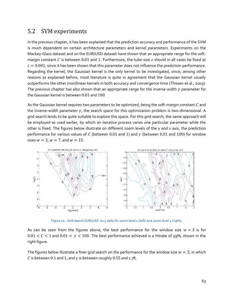
63

5.2 SVM experiments

In the previous chapter, it has been explained that the prediction accuracy and performance of the SVM

is much dependent on certain architecture parameters and kernel parameters. Experiments on the

Mackey-Glass dataset and on the EUR/USD dataset have shown that an appropriate range for the soft-

margin constant is between and . Furthermore, the tube-size should in all cases be fixed at

, since it has been shown that this parameter does not influence the prediction performance.

Regarding the kernel, the Gaussian kernel is the only kernel to be investigated, since, among other

reasons as explained before, most literature is quite in agreement that the Gaussian kernel usually

outperforms the other (non)linear kernels in both accuracy and convergence time (Thissen et al., 2003).

The previous chapter has also shown that an appropriate range for the inverse-width parameter for

the Gaussian kernel is between and .

As the Gaussian kernel requires two parameters to be optimized, being the soft-margin constant and

the inverse-width parameter , the search space for this optimization problem is two-dimensional. A

grid search lends to be quite suitable to explore this space. For this grid search, the same approach will

be employed as used earlier, by which an iterative process varies one particular parameter while the

other is fixed. The figures below illustrate on different zoom levels of the y and x axis, the prediction

performance for various values of (between and ) and (between and ) for window

sizes , and .

Figure 22 - Grid search EUR/USD w=3 daily for zoom level 1 (left) and zoom level 2 (right).

As can be seen from the figures above, the best performance for the window size is for

and . The best performance achieved is a hitrate of 59%, shown in the

right figure.

The figures below illustrate a finer grid search on the performance for the window size , in which

is between and , and is between roughly and 1.78.

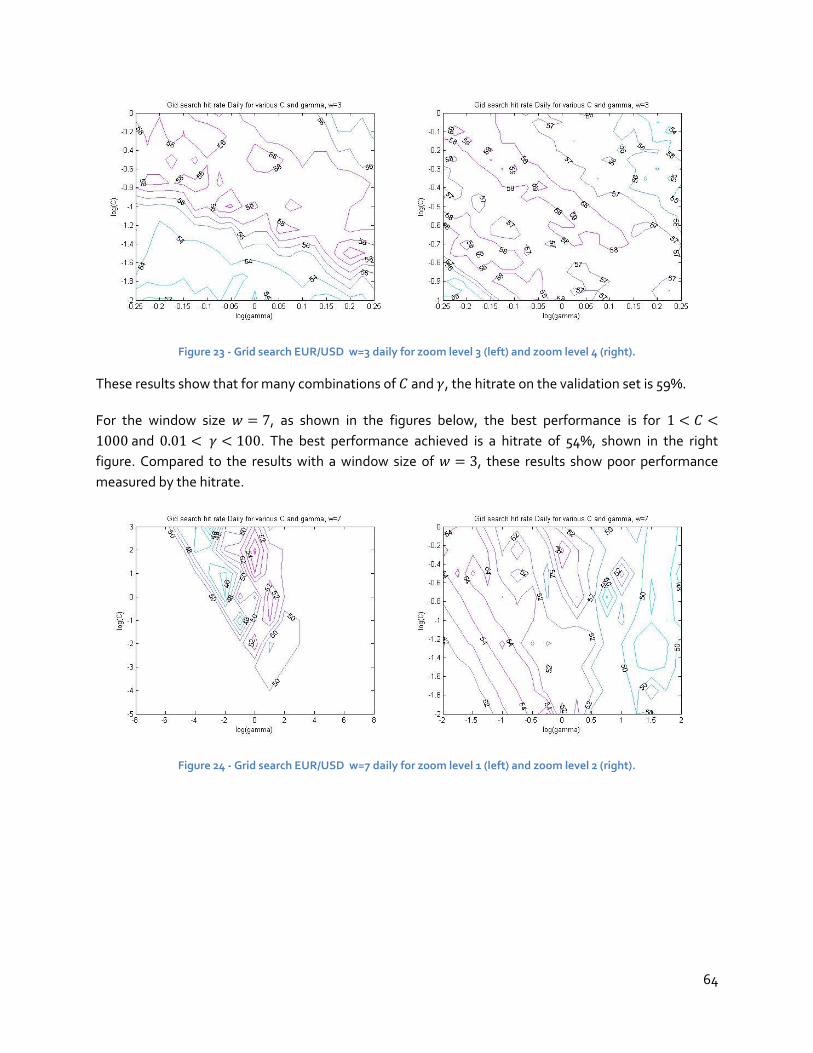
64

Figure 23 - Grid search EUR/USD w=3 daily for zoom level 3 (left) and zoom level 4 (right).

These results show that for many combinations of and , the hitrate on the validation set is 59%.

For the window size , as shown in the figures below, the best performance is for

and . The best performance achieved is a hitrate of 54%, shown in the right

figure. Compared to the results with a window size of , these results show poor performance

measured by the hitrate.

Figure 24 - Grid search EUR/USD w=7 daily for zoom level 1 (left) and zoom level 2 (right).

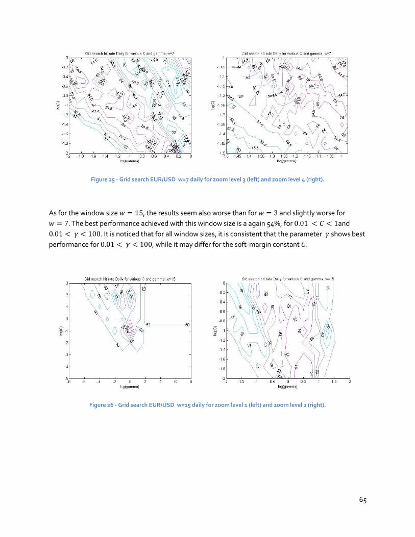
65

Figure 25 - Grid search EUR/USD w=7 daily for zoom level 3 (left) and zoom level 4 (right).

As for the window size , the results seem also worse than for and slightly worse for

The best performance achieved with this window size is a again 54%, for and

. It is noticed that for all window sizes, it is consistent that the parameter shows best

performance for , while it may differ for the soft-margin constant .

Figure 26 - Grid search EUR/USD w=15 daily for zoom level 1 (left) and zoom level 2 (right).

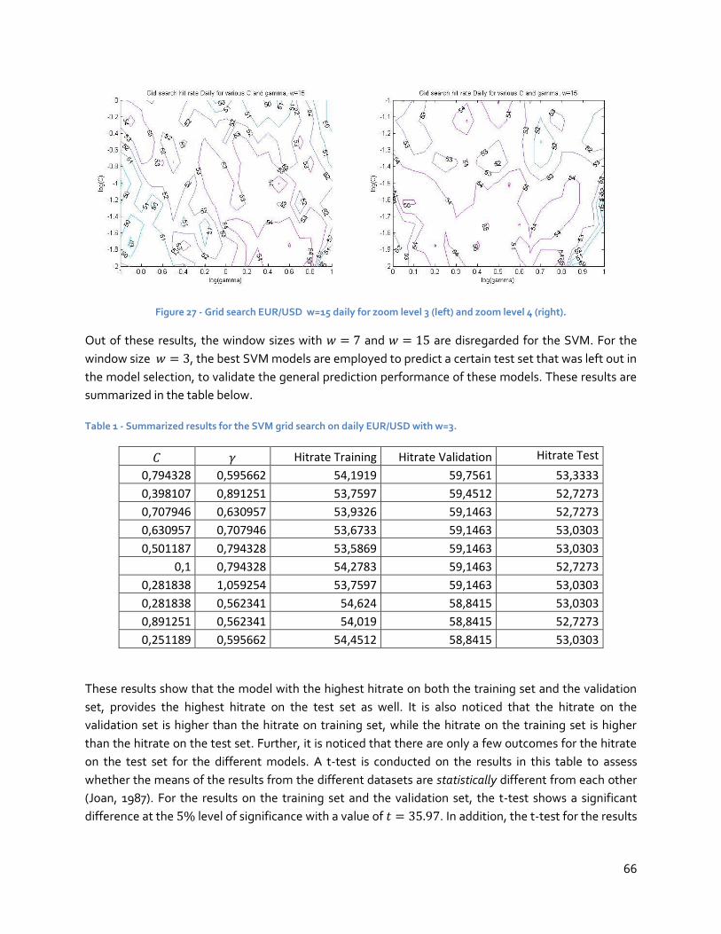
66

Figure 27 - Grid search EUR/USD w=15 daily for zoom level 3 (left) and zoom level 4 (right).

Out of these results, the window sizes with and are disregarded for the SVM. For the

window size , the best SVM models are employed to predict a certain test set that was left out in

the model selection, to validate the general prediction performance of these models. These results are

summarized in the table below.

Table 1 - Summarized results for the SVM grid search on daily EUR/USD with w=3.

Hitrate Training Hitrate Validation Hitrate Test

0,794328 0,595662 54,1919 59,7561 53,3333

0,398107 0,891251 53,7597 59,4512 52,7273

0,707946 0,630957 53,9326 59,1463 52,7273

0,630957 0,707946 53,6733 59,1463 53,0303

0,501187 0,794328 53,5869 59,1463 53,0303

0,1 0,794328 54,2783 59,1463 52,7273

0,281838 1,059254 53,7597 59,1463 53,0303

0,281838 0,562341 54,624 58,8415 53,0303

0,891251 0,562341 54,019 58,8415 52,7273

0,251189 0,595662 54,4512 58,8415 53,0303

These results show that the model with the highest hitrate on both the training set and the validation

set, provides the highest hitrate on the test set as well. It is also noticed that the hitrate on the

validation set is higher than the hitrate on training set, while the hitrate on the training set is higher

than the hitrate on the test set. Further, it is noticed that there are only a few outcomes for the hitrate

on the test set for the different models. A t-test is conducted on the results in this table to assess

whether the means of the results from the different datasets are statistically different from each other

(Joan, 1987). For the results on the training set and the validation set, the t-test shows a significant

difference at the level of significance with a value of . In addition, the t-test for the results

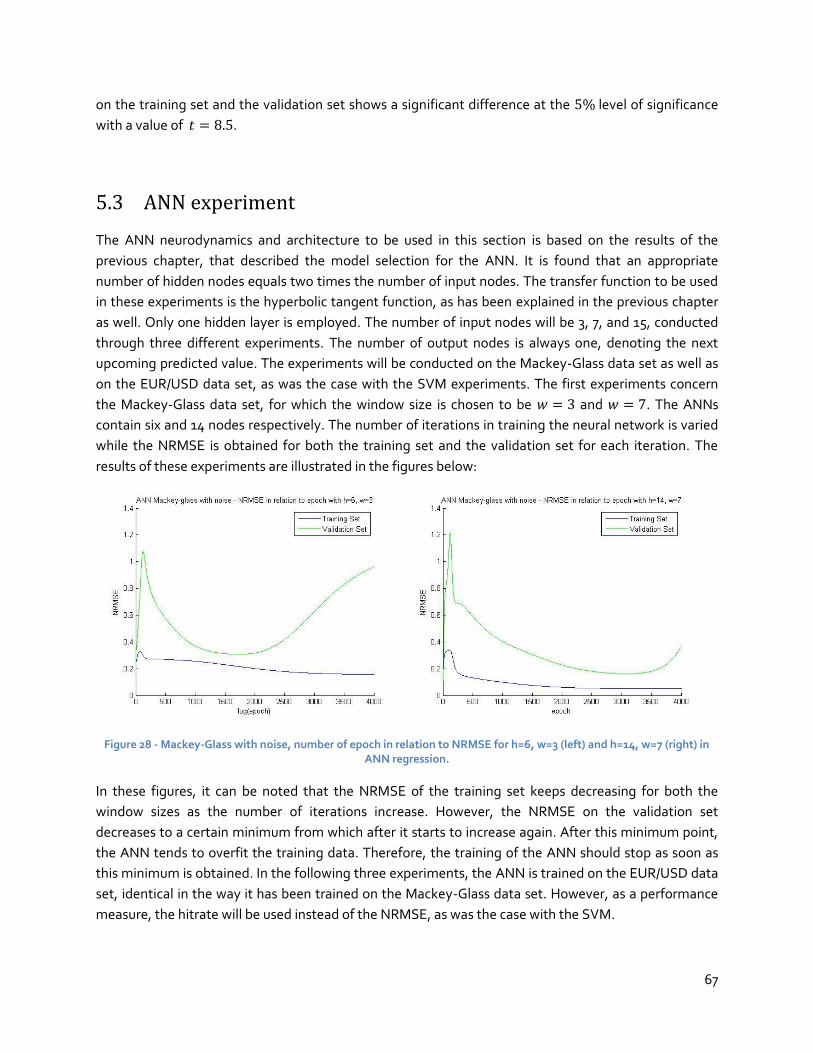
67

on the training set and the validation set shows a significant difference at the level of significance

with a value of .

5.3 ANN experiment

The ANN neurodynamics and architecture to be used in this section is based on the results of the

previous chapter, that described the model selection for the ANN. It is found that an appropriate

number of hidden nodes equals two times the number of input nodes. The transfer function to be used

in these experiments is the hyperbolic tangent function, as has been explained in the previous chapter

as well. Only one hidden layer is employed. The number of input nodes will be 3, 7, and 15, conducted

through three different experiments. The number of output nodes is always one, denoting the next

upcoming predicted value. The experiments will be conducted on the Mackey-Glass data set as well as

on the EUR/USD data set, as was the case with the SVM experiments. The first experiments concern

the Mackey-Glass data set, for which the window size is chosen to be and . The ANNs

contain six and 14 nodes respectively. The number of iterations in training the neural network is varied

while the NRMSE is obtained for both the training set and the validation set for each iteration. The

results of these experiments are illustrated in the figures below:

Figure 28 - Mackey-Glass with noise, number of epoch in relation to NRMSE for h=6, w=3 (left) and h=14, w=7 (right) in ANN regression.

In these figures, it can be noted that the NRMSE of the training set keeps decreasing for both the

window sizes as the number of iterations increase. However, the NRMSE on the validation set

decreases to a certain minimum from which after it starts to increase again. After this minimum point,

the ANN tends to overfit the training data. Therefore, the training of the ANN should stop as soon as

this minimum is obtained. In the following three experiments, the ANN is trained on the EUR/USD data

set, identical in the way it has been trained on the Mackey-Glass data set. However, as a performance

measure, the hitrate will be used instead of the NRMSE, as was the case with the SVM.

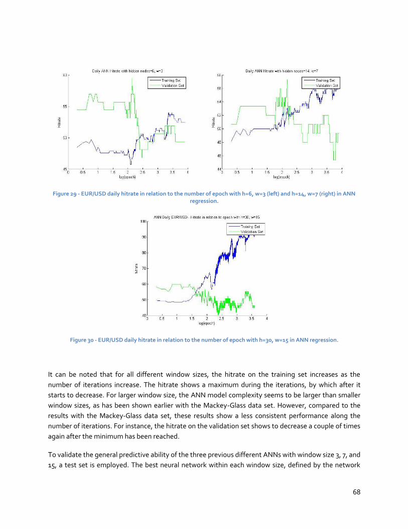
68

Figure 29 - EUR/USD daily hitrate in relation to the number of epoch with h=6, w=3 (left) and h=14, w=7 (right) in ANN regression.

Figure 30 - EUR/USD daily hitrate in relation to the number of epoch with h=30, w=15 in ANN regression.

It can be noted that for all different window sizes, the hitrate on the training set increases as the

number of iterations increase. The hitrate shows a maximum during the iterations, by which after it

starts to decrease. For larger window size, the ANN model complexity seems to be larger than smaller

window sizes, as has been shown earlier with the Mackey-Glass data set. However, compared to the

results with the Mackey-Glass data set, these results show a less consistent performance along the

number of iterations. For instance, the hitrate on the validation set shows to decrease a couple of times

again after the minimum has been reached.

To validate the general predictive ability of the three previous different ANNs with window size 3, 7, and

15, a test set is employed. The best neural network within each window size, defined by the network

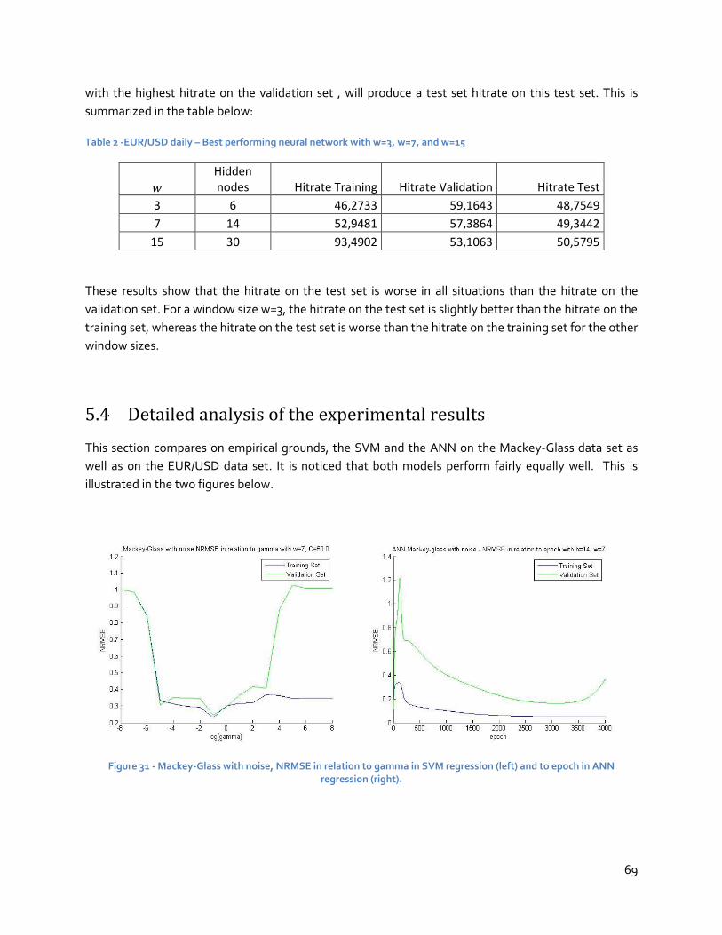
69

with the highest hitrate on the validation set , will produce a test set hitrate on this test set. This is

summarized in the table below:

Table 2 -EUR/USD daily – Best performing neural network with w=3, w=7, and w=15

Hidden nodes Hitrate Training Hitrate Validation

Hitrate Test

3 6 46,2733 59,1643 48,7549

7 14 52,9481 57,3864 49,3442

15 30 93,4902 53,1063 50,5795

These results show that the hitrate on the test set is worse in all situations than the hitrate on the

validation set. For a window size w=3, the hitrate on the test set is slightly better than the hitrate on the

training set, whereas the hitrate on the test set is worse than the hitrate on the training set for the other

window sizes.

5.4 Detailed analysis of the experimental results

This section compares on empirical grounds, the SVM and the ANN on the Mackey-Glass data set as

well as on the EUR/USD data set. It is noticed that both models perform fairly equally well. This is

illustrated in the two figures below.

Figure 31 - Mackey-Glass with noise, NRMSE in relation to gamma in SVM regression (left) and to epoch in ANN regression (right).

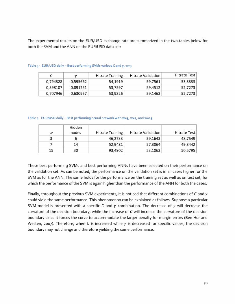
70

The experimental results on the EUR/USD exchange rate are summarized in the two tables below for

both the SVM and the ANN on the EUR/USD data set:

Table 3 - EUR/USD daily – Best performing SVMs various C and γ, w=3

Hitrate Training Hitrate Validation Hitrate Test

0,794328 0,595662 54,1919 59,7561 53,3333

0,398107 0,891251 53,7597 59,4512 52,7273

0,707946 0,630957 53,9326 59,1463 52,7273

Table 4 - EUR/USD daily – Best performing neural network with w=3, w=7, and w=15

Hidden nodes Hitrate Training Hitrate Validation

Hitrate Test

3 6 46,2733 59,1643 48,7549

7 14 52,9481 57,3864 49,3442

15 30 93,4902 53,1063 50,5795

These best performing SVMs and best performing ANNs have been selected on their performance on

the validation set. As can be noted, the performance on the validation set is in all cases higher for the

SVM as for the ANN. The same holds for the performance on the training set as well as on test set, for

which the performance of the SVM is again higher than the performance of the ANN for both the cases.

Finally, throughout the previous SVM experiments, it is noticed that different combinations of and

could yield the same performance. This phenomenon can be explained as follows. Suppose a particular

SVM model is presented with a specific and combination. The decrease of will decrease the

curvature of the decision boundary, while the increase of will increase the curvature of the decision

boundary since it forces the curve to accommodate the larger penalty for margin errors (Ben Hur and

Westen, 2007). Therefore, when is increased while is decreased for specific values, the decision

boundary may not change and therefore yielding the same performance.

71

72

6 Reflection

This chapter reflects upon the conducted literature review and on the empirical results in the previous

chapters, with respect to the research objective.

The main research objective is formulated as follows:

This research aims to propose a prediction model that is able to accurately predict exchange rate

movements, thereby acting as a decision-support aid for firms and investors, providing them the necessary

knowledge to better anticipate possible future exchange rate movements.

The question is, did the SVM or the ANN, theoretically or empirically, proved to be able to accurately

predict exchange rate movements? On theoretical grounds, SVMs as well as the ANNs have in some

cases shown to be effective in forecasting the currency market, although not all researchers agree

(Andreou and Zombanakis ,2006; Dunis et al, 2008; Müller et al., 1997, Mukherjee, Osuna and Girosi,

1997; Huang, 2008; Liu and Wang, 2007; Kim , 2002; Tay and Cao, 2000).

However, on empirical grounds of this research, the answer is not so straightforward. When the figures

and the tables in the experiments for the SVM and the ANN are examined more closely, certain

unexpected outcomes are observed. For instance, the hitrate on the training set for the SVM is in all

three cases lower than the hitrate on the validation set. For the ANN, this phenomenon occurs in the

first two cases. This observation supports the notion that there might be much noise within this

dataset. Even stronger, that a large portion of this data set can be denoted as a random process.

Comparing the results of this research with previous conducted research is rather difficult, since many

different performance measures are used throughout the literature concerning financial forecasting. In

addition, not much research has been conducted yet on the application of SVMs in exchange rate

prediction. Nevertheless, Kim (2003) has used exactly the same performance measure as in this

research, namely the hitrate, in examining the prediction performance of support vector machines on

stock markets. The results by Kim (2003) resemble the results in this research quite well, with hitrates

around the 56%. His main conclusion is that the SVM is a favorable alternative to the ANN for financial

forecasting, even though the results may have shown to be less promising.

When the empirical findings are reflected back upon the conducted literature review that investigated

whether financial markets are susceptible to forecasting, the theoretical argument of the efficient

market hypothesis plays an important role. This hypothesis states that a particular market is said to be

efficient, if all the participants and actors related to that market receive all the possible information at

any time and at the same time (Malkiel, 1987). As a consequence, the price in such a market will only

move at the arrival of new information, which is by definition impossible to forecast on only historical

data. Although it has been shown by some researchers that financial forecasting does hold a predictive

ability and profitability (Sweeney, 1988; Brock., Lakonishok, LeBaron, 1992; Bessembinder and Chan,

73

1995; Huang, 1995; Raj and Thurston, 1996), within the limitations of this research, the efficient market

hypothesis can however not be falsified based on the conducted experiments in the previous chapter.

Furthermore, since the aim of this research was not to compare the SVM and the ANN in general but

very specific on the EUR/USD exchange rate, the results as presented in the previous chapter on the

Mackey-Glass data set are not enough to reach a solid conclusion regarding the general performance.

Further comparisons have to be made with an increasing noisy component on the Mackey-Glass data

set to understand which model is most successful in deriving structure from the inherent noise.

Finally, in light of providing firms and investors the necessary knowledge to act accordingly on possible

future exchange rate movements, the SVM prediction model may still be used as a decision-support aid

for this particular purpose. While the predictions on their own as provided by the SVM are not

necessarily accurate, they may provide some added value in combination with other models. In

addition, users of the model may learn to interpret the predictions in such a way, that they still signal

some sort of relevant information. The decision-support aid would be the SVM prediction model

wrapped in an IT system that provides predicted probabilities whether a specific currency will rise, fall,

or remain unchanged. Firms may use this information to decide, for instance, upon the quantity of

importing goods. Since importing requires a currency exchange from one currency to the other, it

might be beneficial to import more goods than usual when the home currency is predicted to rise, and

thereby reducing the import costs. Likewise, investors are able to better anticipate on price

fluctuations, and adjusting their portfolio on the obtained predictions to achieve a higher return on

investment.

74

7 Conclusions

Based on the conducted literature review in the earlier chapters, as well as on empirical results of the

experimentation’s chapter in which experiments has been conducted on the Mackey-Glass data set and

the EUR/USD data set using SVMs and ANNs, this chapter aims to provide conclusions on the posed

research questions. Furthermore, the limitations of this research are given, as well as suggestions for

future research.

7.1 Answers to the Research Questions

The first research question concerns the possibilities within exchange rate prediction, which has been

explored in the literature review. It has been shown that there exist many different methods for

forecasting financial markets in general and the exchange market in particular. Common market

structure trading rules in technical analysis, such as the filter rule, the moving average cross over rule,

and Bollinger bands have been described. Empirical evidence from the application of these forecasting

models on various financial markets, as well as empirical evidence in favor and against the efficient

market hypothesis, has shown that it is at least evident that there is some sort of interest in trying to

forecast the financial markets, and at most safe to consider that it might indeed be possible. The

traditional linear forecasting methods as presented earlier suffer from their linear nature, since

empirical evidence has demonstrated the existence of nonlinearities in exchange rates. In addition, the

usefulness of the parametric nonlinear models is restricted, since their pre-specification limits them to

capture all the possible nonlinear patterns. The few nonparametric nonlinear models proposed to

exchange rate prediction seemed to show poor performance. For these reasons, the use of

computational intelligence in predicting the exchange rate is investigated, in which these previously

mentioned limitations may be overcome

This exploration of computational intelligence techniques was limited to the ANN and the SVM. It has

been shown that an important feature of these models is their ability to generalize through nonlinear

approximation and interpolation in usually high-dimensional spaces (Kecman, 2001). Generalization

refers to the capacity of the model to provide correct outputs when using data that were not seen

during training. This feature is extremely useful in financial forecasting, since the underlying

mechanisms within the financial market are often unknown or hard to describe (Zhang, Patuwo, Hu,

1998). However, one problem with these models is that the underlying laws governing the system to be

modeled, and from which the data is generated, in this case the exchange market, is not always clear.

An important feature of ANNs, is that they are considered to be universal functional approximators,

thus being able to approximate any continuous function to any desired accuracy (Irie and Miyake, 1988;

Hornik et al., 1989; Cybenko, 1989; Funahashi, 1989; Hornik, 1991, 1993). Problems with ANNs are their

excessive training times, the dangers of underfitting and overfitting, and that they require the selection

of a large number of controlling parameters, for which there is no structured way or method to obtain

the most values for a given task (Huang et al.,2004).

75

A basic understanding in the crucial elements of the SVM was provided, with concepts such as the

decision boundary, the hyperplane, the discriminant function, the geometric margin, the amount of

slack, the error function, the dual representation, and the kernel function. The basic idea of the SVM is

finding a maximum margin classifier that separates a training set into positive and negative classes,

based on a discriminant function that maximizes the geometric margin. Finding that specific

discriminant function is shown to be equivalent to solving a constrained optimization problem. The

dual formulation of the SVM using the method of Langrage multipliers (Cortes and Vapnik, 1995;

Shölkopf and Smola, 2002; Christianini and Shawe-Taylor, 2000), makes it possible to perform a

nonlinear transformation and a large margin separation in the high-dimensional feature space. An

important consequence of the dual representation and the kernel function is that the dimension of the

feature space does not need to affect the computational complexity. In addition, the solution that is

found by the optimization problem has certain interesting properties. It has been proven that the

obtained solution is always global, since the problem formulation is convex (Burges, C.J.C., 1998).

Furthermore, given the fact that the discriminant function is strictly convex, it follows that the obtained

solution is also unique. These properties make overfitting unlikely to occur with the SVM. This is also an

important difference with the ANN. The SVM is designed to minimize the structural risk by minimizing

an upper bound of the generalization error,contrary to ANNs that tend to minimize the empirical risk by

minimizing the training error. Therefore, an SVM is less vulnerable to either overfitting or underfitting.

The second research question concerns the input selection for the ANN and the SVM and how this input

is preprocessed. Based on literature review, certain steps to properly prepare the data have been

undertaken, by which one can attain an increase in the prediction performance and in the learning

speed. These steps are sampling, transforming, normalizing, dividing, and windowing. The sample size

has been chosen to be 6 1/2 years, while the sampling rate has been chosen to be daily. The data was

then transformed by taking successive variations of the data, also known as the return. Subsequently,

the data was normalized to -1 and 1. Afterwards, the data was divided into three subsets, 70% for the

training set, 20% for the validation set, and 10% for the testing set. Finally, the window size is chosen to

be varied for a window size of 3, 7, and 15.

The third research question concerns the output selection and how this output is interpreted. The output

as a performance measure in this research solely depends on accuracy, which is measured by the

NRMSE and the hitrate. Comparing two models will be based on comparing the performance on the

test set.

The fourth research question concerns how to approach the model selection for both the SVM and the

ANN. The model selection was chosen to be based on the bias-variance dilemma, which denotes the

trade-off between the amount of variation within different estimators on different values of a specific

data set (variation) and the difference between the estimator’s expected value and the true value of the

parameter being estimated (bias). The variance of the model increases with model complexity, while

the bias of the model decreases with model complexity. Regarding the SVM, it has been found that the

increase of the tube size Increases the bias and decreases the variance, leading to a lower model

complexity. The increase of the soft-margin constant decreases the bias and increases the variance,

leading to a higher model complexity. Furthermore, for the Gaussian kernel, it has been found that the

76

inverse width parameter increases the model complexity of the SVM. Regarding the ANN, it has been

found that the increase of the number of hidden layers and the neurons within these hidden layers

decreases the bias and increases the variance, leading to a higher model complexity.

It has been found that for the following experiments, an appropriate range for the soft-margin constant

is between and , the tube size epsilon is set on a default value of , and an appropriate

range for the inverse-width kernel parameter is between and . In addition, the gaussian

kernel function is used in all experiments. Regarding the ANN, the hyperbolic tangent function is used

as the activation function, while the number of hidden nodes is two times the window size, i.e. 6 hidden

nodes for a window size of 3 and 14 hidden nodes for a window size of 7.

The fifth research question concerns which of the two models, the SVM and the ANN, performed best in

forecasting the EUR/USD exchange rate. This research question is answered through both theoretical

findings and experimental results. On theoretical grounds, it has at least been shown that SVMs have a

few interesting properties which may support the notion that SVMs generally perform better than

ANNs. One important property is that there are fewer free parameters to tune for the SVM compared

to the neural network. The SVM used in this research, with a Gaussian kernel, requires only three free

parameters, namely , and , to be tuned while ANNs require a larger number of controlling

parameters, including the number of hidden layers, the number of hidden nodes, learning rate, the

momentum term, the number of iterations, transfer functions, and weights initialization methods. For

both models, it is a difficult task to obtain an optimal combination of parameters which produces the

best prediction performance. As has been shown, these optimal combinations are found empirically.

Thereby it became clear that the less free parameters that need to be tuned, the easier it is to obtain an

optimal combination. Another interesting property that was found for SVMs is that training an SVM is

equivalent to solving a linearly constraint quadratic programming problem, and that the solution of the

SVM is unique, optimal and global. This is however not the case for the neural network, which may not

converge to global solutions.

However, on empirical grounds based on experimentation results in chapter 6, no solid conclusion can

be drawn regarding which model performed the best on the EUR/USD data set. The main research

question can therefore be answered that, on this data set at least, the SVM has not shown to be more

practically feasible in terms of prediction accuracy than an ANN. Nevertheless, in light of providing

firms and investors the necessary knowledge to act accordingly on possible future exchange rate

movements, the SVM prediction model may still be used as a decision-support aid for this particular

purpose. While the predictions on their own as provided by the SVM are not necessarily accurate, they

may provide some added value in combination with other models. In addition, users of the model may

learn to interpret the predictions in such a way, that they still signal some sort of relevant information.

77

7.2 Limitations

The limitations of this research are inherently linked to the narrow research scope, which limited the

exploration of various models on various data sets. This was due to the constrained research time and

the complexity of the various additional models in that exploring these models would require an

extensive research on its own. To start with, this research has only explored technical analysis, while

fundamental analysis might have provided a better prediction performance. Regarding the

fundamental analysis, one could think of incorporating news events as input to the prediction models.

The models themselves might have been of a totally different nature than the ones used in this

research, being the SVM and the artificial neuron network. A few of these models have been briefly

described in the literature review section. Again, the reason why these models have not been

investigated thoroughly as compared to the SVM, is partly justified by the constrained research time

and partly by the subjective interest for SVM to choose this model above other models. Regarding the

SVM and the ANN, limited variations of these models have been explored while there do exist many

forms of these models. For instance, the SVM might have been employed with a totally different kernel

function, or a combination of various kernel functions all together. Likewise, the ANN as employed in

this research is a multilayer perceptron, while different structures than this one might have proved to

be better performing for the purpose of this research.

The data set was also limited in the sense that on one hand the data set itself was only limited to a

specific period of time being six years, while on the other hand more data sets (as in more exchange

rates) might have been explored. However, it has been shown by literature review that a period of six

years seems reasonable enough for the purpose of exchange rate prediction. In addition, exploring

various exchange rates would not necessarily mean gaining a better understanding of whether SVMs

perform better than ANNs in exchange-rate prediction in general. The reason is that these exchange

rates might have different characteristics that each requires a different SVMs in terms of model

structure, leading to several conclusions that may prove hard to be combined for general exchange-rate

prediction.

As for the validity of the research results, the conclusions regarding the best performing model on the

used data set is only valid to a certain extent. The reason is that model selection has been based on the

performance on the validation set, and the best performing model has been based on the performance

on the test set, while one might base the best performing model on a different dataset. In addition, the

conclusion is only valid on the previous six years, while it may differ on future data from this specific

exchange rate.

78

7.3 Future Research

This research has shown that SVMs offer some advantages in comparison to ANNs in financial

forecasting. Future research may explore the possibility of refining the SVM in order to achieve a higher

generalization performance.

Refining the SVM may lie in finding a better structure in terms of the kernel function, which might be a

combination of various kernels. It might also lie in how the free parameters for the SVM are selected,

perhaps by an alternative computational intelligence method. This would require further research on

the topic that points to the direction of genetic algorithms in combination with SVMs (Lessmann et

al.,2007). By imitating the biological evolution process, genetic algorithms try to find optimal or new

optimal solutions with relatively modest computational requirements.

In addition, modified SVMs might provide a better performance that would therefore lend themselves

to future research. For instance, Cao and Tay (2001) have studied the performance of a C-Ascending

SVM in financial time series forecasting, which are SVMs with an adopting soft margin constant by a

specific weight function. Likewise, further research may lie in for instance least-squares SVMs as

opposed to the standard SVM. Wang and Liu (2008) have explored the performance prediction of least-

squares SVMs in exchange rate prediction with promising results. The least-squares SVM is an

improved algorithm based on the SVM (Vapnik, 1998).

Alternatively, future research may be conducted on combining different inputs from various data

sources to an SVM prediction model. One could thereby think of inputs from various macroeconomic

indicators that might have an effect on the exchange rate.

A completely different direction that one may take in exchange rate prediction, is shifting the research

towards fundamental analysis, or at least a combination between fundamental analysis and technical

analysis. As this research has shown, at least on the methods used and on the specific EUR/USD

dataset, technical analysis has not fully delivered the desired results, leaving room for fundamental

analysis to accomplish more promising results. Still, future research on fundamental analysis may be

incorporated with the use of SVMs, in for instance pattern recognition in economic news events,

thereby building up on the knowledge gained in this research.

79

80

References

Almeida, A., Goodhart, C., Payne, R., (1998). The effects of macroeconomic news on high frequency exchange rate behavior. Journal of Financial and Quantitative Analysis 33 (3), 383e408. Andersen, T., Bollerslev, T., (1998). Deutsche markedollar volatility: intraday activity patterns,

macroeconomic announcements, and longer run dependencies. Journal of Finance 53, 219e265.

Andersen, T., Bollerslev, T., Diebold, F., Vega, C., (2003). Micro effects of macro announcements: real-time price discovery in foreign exchange. American Economic Review 9, 38e62. Alexander S. S. (1964). Price Movements in Speculative Markets: Trends or Random Walks, No. 2. In: Cootner P. (Ed.) The Random Character of Stock Prices. MIT Press, Cambridge, 338–372 Allen F., Karjalainen R. (1999). Using Genetic Algorithms to Find Technical Trading Rules. Journal Finance Economics 51, 245–271

Ayat, N. E., Cheriet, M. and Suen C. Y. (2005). Automatic model selection for the optimization of SVM

kernels. Pattern Recognition, vol. 38, pp. 1733-1745, 2005.

Appel, Gerald (1999). Technical Analysis Power Tools for Active Investors. Financial Times Prentice Hall. pp. 166. Andreou, A.S., Zombanakis, G.A., (2006). Computational intelligence in exchange rate forecasting. Bank of Greece. Achelis S. B. (1995) Technical Analysis from A to Z. Probus Publishing,Chicago.

Azoff, E.M.,(1994). Neural Network Time Series Forecasting of Financial Markets. John Wiley and Sons,

Chichester.

Baum, E.B. and Haussler, D.,(1989). What size net gives valid generalization? Neural Computational. 6

151-160.

Bellgard, C. and Goldschmidt, P. (1999). Forecasting Across Frequencies: Linearity

and Non-Linearity. University of Western Australia Research Paper, Proceedings of the

International Conference on Advanced Technology, Australia.

Ben Hur, A., Weston, J. (2007). A user’s guide to support vector machines. Department of computer

science, Colorado State University.

Beran, J. and Ocker, D. (1999). SEMIFAR forecasts, with applications to foreign exchange rates. Journal of

Statistical Planning and Inference, Vol.80, pp.137-153.

81

Bilson, J.F.O. (1992). Technical currency trading. Chicago, I 11; The Chicago Corporation.

Blanz, V. Scholkopf B., Bulthoff H., Burges C., Vapnik V., and Vetter T. (1996).Comparison of view-based

object recognition algorithms using realistic 3-D models. artificial neural networks – ICANN’96 pages 251 -

256, BerlinSpringer lecture Notes in computer science,Vol. 1112.

Bodt, E., Rynkiewicz, J., Cottrell, M. (2001). Some known facts about financial data. European

symposium on artificial neural networks 25-27. pp. 223-236.

Boser, B.E., Guyon, I. M., and Vapnik, V. N. (1992). A Training Algorithm for Optimal Margin Classifiers.

Proc. of the 5th Annual Workshop on Computational Learning Theory, Pittsburgh, Pennsylvania, USA.

Burges, C.J.C., and Scholkopf, B. (1997). Improving the accuracy and speed of support vector learning

machines. Advances in neural information processing systems 9, pages 375 -- 318, Cambridge, NA, MIT

press.

Burges, C.J.C. (1998). A tutorial on support vector machines for pattern recognition. Data mining and

knowledge discovery 2, 121-167.

Ben Omrane, W., Bauwens, L., Giot, P. (2005). News announcements, market activity and volatility in the euro/dollar foreign exchange market. Journal of International Money and Finance 24 (7), 1108e1125. Bessembinder H., Chan K. (1995). The Profitability of Technical Trading Rules in the Asian Stock Markets. Pacific Basin Finance Journal 3, 257–284 Bessembinder H., Chan K. (1998). Market Efficiency and the Returns to Technical Analysis. Financial Management 27, 5–17 Brock W., Lakonishok J., LeBaron B. (1992). Simple Technical Trading Rules and the Stochastic Properties of Stock Returns. Journal of Finance 47, 1731–1764 Brown S., Goetzmann W., Ross S. (1995). Survival. Journal of Finance 50, 853–873 Brown S., Goetzmann W., Kumar A. (1998). The Dow Theory: William Peter Hamilton’s Track Record Reconsidered. Working Paper, Stern School of Business, New York University Brock W., Lakonishok J., Le Baron B., (1992). Simple Technical Trading Rules and the Stochastic Properties of Stock Returns, The Journal of Finance, vol. XLVII, n°5, pp. 1731-1764 Bishop, C.M. (2007). Pattern Recognition and Machine Learning. Springer, 2007. Bachelier, L, (1900). Théorie de la spéculation, Gauthier-Villars, Paris, Annales Scientifiques de l’École Normale Supérieure 3 (17): 21–86

82

Ball R. (1978) Filter Rules: Interpretation of Market Efficiency, Experimental Problems and Australian Evidence. Accounting Education 18, 1–17 Brock, W.A.D.A., Hsieh, and B. LeBaron. (1991). Nonlinear dynamics, chaos, and instability. Cambrigde,

Mass.:MIT Press.

Bollerslev, T., (1990). Modeling the coherence in short-run nominal exchange rates: A multivariate generalized ARCH model, Review of Economics and Statistics 72 (1990) 498–505. Burton G. Malkiel (1987). Efficient market hypothesis,The New Palgrave: A Dictionary of Economics322, v. 2, pp. 120–23.

Cortes C. and Vapnik V. (1995). Support vector networks. Machine learning, 20: 273 – 297.

Cristianini, N. and Shawe-Taylor,(2000). J. An introduction to support vector machines and other kernel-

based learning methods. Cambridge: Cambridge University Press.

Chih-Chung Chang and Chih-Jen Lin (2001). LIBSVM: A library for support vector machines. Software available at: http://www.csie.ntu.edu.tw/~cjlin/libsvm

Cheung, Y., Chinn, M., Pascual, A., (2005). Empirical exchange rate models of the nineties: are any fit to survive? Journal of International Money and Finance 24 (7), 1150e1175. Chaboud, A., Chernenko, S., Howorka, E., Iyer, R., Liu, D., Wright, J., (2004). The high-frequency effects of U.S. macroeconomic data releases on prices and trading activity in the global interdealer foreign exchange market. Board of Governors of the Federal Reserve System, IFDP No. 823. Carter R. B., Van Auken H. E. (1990). Security Analysis and Portfolio Management: A Survey and Analysis. Journal of Portfolio Management, Spring, 81–85 Caudill, M., (1992). The view from now. AI expert. Corrado C. J., Lee S. H. (1992). Filter Rule Tests of the Economic Significance of Serial Dependence in Daily Stock Returns. Journal of Financial Research 15, 369–387 Campbell J.Y., Lo A.W. & MacKinlay A.C, (1997)., The Econometrics of Financial Markets, Princeton, New Jersey. Chordia T., Shivakumar L., (2000). Momentum, Business Cycle and Time-Varying Expected Returns, FEN Working Paper Cheng, B., Titterington, D.M., (1994). Neural networks: A review from a statistical perspective. Statistical Science 9 (1), 2–54. Cheng W, Wanger L, Lin CH.,(1996). Forecasting the 30-year US treasury bond with a system of neural networks. Journal of Computational Intelligence in Finance 1996;4:10–6.

83

Cybenko, G., (1989). Approximation by superpositions of a sigmoid neural function. Mathematical Control Signals Systems 2, 303–314. Chappel, D., J. Padmore, P. Mistry and C. Ellis, (1996). A threshold model for French franc/Deutsch mark exchange rate, Journal of Forecasting 15 155–164.

Diebold. F.X. and Nason, J.A., (1990). Nonparametric exchange rate prediction. Journal of

International Economics 28 (1990) 315–322.

Dunis, Williams (2002). Modelling and Trading the EURUSD Exchange Rate, Do Neural Network Models

Perform Better

Dunis, C.L., Laws, J., Sermpinis, G. (2008). Higher order and recurrent Neural architectures for trading the

EUR/USD exchange rate. Liverpool business school.

El-Shazly, M. R. and El-Shazly, H. E. (1997). Comparing the forecasting performance of neural networks

and forward exchange rates. Journal of Multinational Financial Management

Volume 7, Issue 4, Pages 345-356

EddelButtel, D. and McCurdy, T.H.(1998). The impact of news on foreign exchange rates: evidence from

high-frequency data. University of Toronto.

Ederington, L., Lee, J., (1995). The short-run dynamics of price adjustment to new information. Journal of Financial and Quantitative Analysis 30, 117e134. Engelbrecht, A.P., Cloete, I., Geldenhuys, J., Zurada, J.M., (1994). Automatic scaling using gamma learning for feedforward neural networks. Anderson, D.Z. (Ed.), Neural Information Processing Systems, American Institute of Physics, New York, pp. 374–381.

Fernandez-Rodriguez, F., Sosvilla-Rivero, S. and J. Andrada-Felix, J. (1999). Exchange rate forecasts with

simultaneous nearest-neighbor methods: evidence from the EMS. International Journal of Forecasting,

Vol.15, pp.383-392.

Faust, J., Rogers, J., Wang, S., Wright, J., (2003). The high-frequency response of exchange rates and interest rates to macroeconomics announcements. Board of Governors of the Federal Reserve System, IFDP No. 784. Flood, R., Rose, A., (1995). Fixing exchange rates: a virtual quest for fundamentals. Journal of Monetary Economics 36, 3e37. Fama E., Blume M. (1966). Filter Rules and Stock Market Trading. Journal of Business 39, 226–241 Fama E., (1965). The Behavior of Stock Market Prices, Journal of Business, 38, p.34-105 Fama, E., (1965). Random Walks In Stock Market Prices. Financial Analysts Journal 21 (5): 55–59.

84

Fang, H.,L. S.Lai, and M.Lai. (1994). Fractal structure in currency futures price dynamics. Journal of futures markets 14:169-181. Funahashi, K.,(1989). On the approximate realization of continuous mappings by neural networks. Neural Networks 2, 183–192. Grauwe de, P., H. Dewachter, and M.Embrechts. (1993). Exchange rate theory. Chaotic models of foreign

exchange markets. London: Blackwell.

Granger, C.W.J., (1993). Strategies for modelling nonlinear time series relationships. The Economic Record 69 (206), 233–238. Gennaro de, R., Shrieves, R., (1997). Public information releases, private information arrival, and volatility in the foreign exchange market. Journal of Empirical Finance 4, 295e315. Haykin S. (1999). Neural networks: a comprehensive foundation. Englewood CliKs, NJ: Prentice Hall. Hastie, T., Tibshirani, R., and Friedman, J.H. (2001). The Elements of Statistical Learning. Springer, 2001. Hakkio, C., Pearce, D.K., (1985). The reaction of exchange rates to economic news. Economic Inquiry 23 (4), 621e636. Hecht-Nielsen, R., (1989). Neurocomputing. Addison Wesley, Menlo Park, CA. Hudson R., Dempsey M., Keasey K. (1996). A Note on the Weak Form of Efficiency of Capital Markets: The Application of Simple Technical Trading Rules to the U.K. Stock Markets– 1935-1994. Journal of Banking and Finance 20, 1121–1132. Hsu, C., Chang, C., Lin, C. (2010). A practical guide to support vector classification. Department of Computer Science, National Taiwan University, Taipei 106, Taiwan. Hornik, K., (1991). Approximation capabilities of multilayer feed forward networks. Neural Networks 4, 251–257. Hornik, K., (1993). Some new results on neural network approximation. Neural Networks 6, 1069–1072. Hornik, K., Stinchcombe, M., White, H., (1989). Multilayer feedforward networks are universal approximators. Neural Networks 2, 359–366. Huang, Lai, Mori, Wang (2004) . Forecasting foreign exchange rates with artificial neural networks, a review. International Journal of Information Technology & Decision Making. Vol 3, No 1, 145-165 Huang Y -S. (1995).The Trading Performance of Filter Rules On the Taiwan Stock Exchange. Applied Financial Economics 5, 391–395 Huang, W., Nakamori, Y., and Wang, S.Y. (2002).Using change-point detection to seek

85

optimal training set for neural networks in foreign exchange rates forecasting. International Journal of Computational Intelligence and Organization. Hsieh, D.A., (1989). Modeling heteroscedasticity in daily foreign-exchange rates. Journal of Business and Economic Statistics 7, 307–317.

Irie, B., Miyake, S., (1988). Capabilities of three-layered perceptrons. In: Proceedings of the IEEE International Conference on Neural Networks, I, pp. 641–648. Ito, T., Roley, V., (1987). News from the US and Japan: which moves the yen/dollar exchange rate? Journal of Monetary Economics 19 (2), 255e277. Jamal, A.M., and Sundar, C., (1998). Modeling exchange rates with neural networks, Journal of Applied Business Research 14(1), 1–5. Joan, F.B. (1987). Guinness, Gosset, Fisher, and Small Samples. Statistical Science 2 : 45–52. Kim, K. (2003). Financial time series forecasting using Support Vector Machines. Neurocomputing 55, 307-

319.

Keerthi, S.S. and Lin, C.J. (2003). Asymptotic behaviors of support vector machines with Gaussian kernel. Neural Computation, 15(7):1667{1689.

Kang, S., (1991). An investigation of the use of feedforward neural network for forecasting, PhD Thesis, Kent State University, Kent, OH 44240, USA. Katz, J.O.,(1992). Developing neural network forecasters for trading, Technical Analysis of Stocks and Commodities.

Kecman, V., (2001), Learning and soft computing. The MIT Press Cambridge, Massachusetts London,

England.

Lachtermacher, G., Fuller, J.D., (1995). Backpropagation in time series forecasting. Journal of Forecasting

14, 381–393

LeBaron, B. (1993). Practical comparisons of foreign exchange forecasts. Neural Network World

(November); 779-791.

Lento, C., Gradojevic, N., (2007). The profitability of technical trading rules: a combined signal approach.

Journal of applied business research, volume 23, number 1.

Le and Billy Caseyich, R.M. and L.R. Thomas (1993). The significance of technical trading-rule profits in

the foreign exchange market: A bootstrap approach. Journal of International Money and Finance 12:451-

465

86

Liu, L. and Wang, W. (2008). Exchange Rates Forecastiing with Least Squares SVM. International

Conference on Computer Science and Software Engineering.

Love, R., (2004). First and second moment effects of macro news in high frequency foreign exchange data. Mimeo, FMG, London School of Economics. Love, R.R. Payne, R., (2003). Macroeconomic news, order flows, and exchange rates. Discussion Paper 475, FMG, London School of Economics. Lo A. W., MacKinley A. G. (1990) Data Snooping Biases in Tests of Financial Asset Pricing Models. The Review of Financial Studies 3, 431–467 Lessmann, S., Stahlbock, R., Crone, S.F., (2006). Genetic Algorithms for SVM Model Selection . International Joint Conference on Neural Networks Sheraton Vancouver Wall Centre Hotel, Vancouver, BC, Canada. LeCun, Y., Jackel, L., Bottou, L., Brunot, A. Cortes, C., Denker, J., Drucker, H., Guyon, I., Muller, U., Sackinger, E., Simard, P. and Vapnik ,V. (1995). Comparison of Learning Algorithms for Handwritten Digit Recognition. International Conference on artificial neural networks, Ed. F. Fogelman, P. Gallinari, pp. 53-60 Lo A., MackKinlay A.C.(1990). Data-snooping Biases in Tests of Financial Asset Pricing Models, The Review of Financial Studies, vol. 3, p. 431-467. Lin, H.T. and Lin, C.J. (2003). A study on sigmoid kernels for SVM and the training of non-PSD kernels by SMO-type methods. Technical report, Department of Computer Science, National Taiwan University. Lapedes, A., Farber, R.,(1988). How neural nets work. In: Anderson, D.Z., (Ed.), Neural Information Processing Systems, American Institute of Physics, New York, pp. 442–456.

Mukherjee,S., E.Osuna, F. Giroso. (1997). Nonlinear prediction of chaotic time series using SVM. In

proceedings of the IEEE workshop on neural networks for signal processing 7, pages 511 - 519, Amelia

Island FL.

Melvin, M., Yin, X., (2000). Public information arrival, exchange rate volatility, and quote frequency. Economic Journal 110, 644e661. Meese, R., Rogoff, K., (1983a). Empirical exchange rate models of the seventies. Journal of International Economics 14, 3e24. Meese, R., Rogoff, K., (1983b). The out-of-sample failure of empirical exchange rate models. In: Frenkel, J. (Ed.), Exchange Rate and International Macroeconomics. University of Chicago Press, Chicago. Neuroph (2010). Java neural network framework. Source: http://neuroph.sourceforge.net/

87

Meese, R. A. and Rose,A.,(1991). An empirical assessment of non-linearities in models of exchange rate determination. Review of Economic Studies 58 601–619. Mizrach, B.,(1992). Multivariate nearest-neighbor forecasts of EMS exchange rates. Journal of Applied Econometrics 7 , S151–S164. Monica Lam (2004). Neural network techniques for financial performance prediction: integrating fundamental and technical analysis, Volume 37, Issue 4, Data mining for financial decision making,Pages 567-581. Müller, K. R. , Smola, A., Rätsch, G., Schölkopf, B., Kohlmorgen, J., and Vapnik, V. (1997).Predicting

time series with support vector machines. In proceedings of the IEEE workshop on neural networks for

signal processing 7, pages 511 – 519, Amelia Island FL.

Malkiel B. (1995) .A Random Walk Down Wall Street, 6th edn. W. W. Norton, New York Murphy, J. J. (1999). Technical Analysis of the Financial Markets. New York Institute of Finance.

Murphy, J. J. (2000). Charting Made Easy. Marketplace Books (Wiley). Mood, A.; Graybill, F.; Boes, D. (1974). Introduction to the Theory of Statistics (3rd ed.). McGraw-Hill. p. 229. Mehta, M. (1995), ‘Foreign Exchange Markets’, 176-198, in A. N. Refenes [ed.], Neural Networks in the Capital Markets, John Wiley, Chichester. Nelson, M., Illingworth, W.T., (1991). A practical guide to neural nets. Addison Wesley, Reading, MA. Nelson, L. and Zimmerman, D.L.,(2004). Testing for directional symmetry in spatial dependence using the periodogram. Wyeth Research, Pearl River, NY 10965, USA. Department of Statistics and Actuarial Science, University of Iowa, 241 Schaeffer Hall, Iowa City, IA 52242, USA. Neely C. J., Weller P., Dittmar R. (1997). Is Technical Analysis in the Foreign Exchange Market Profitable? A Genetic Programming Approach. Journal of Financial Quantitative Analysis 32, 405–426 Oanda Corporation (2010). Historical foreign exchange data . Source: https://fxtrade.oanda.com/trade-

forex/fxtrade/historical-data

Osuna,S., R. Freud, and F. Giroso. (1997). An improved training algorithm for support vector machines. In

proceedings of the 1997 IEEE workshop on neural networks for signal processing. Pages 276 - 285,

Amelia Island, FL.

Peel, D.A., and Yadav, P.(1995).The time series behavior of spot exchange rates in the German hyper-inflation period: Was the process chaotic? Empirical Economics 20 455–463.

88

Pilbeam, K. (2010). Finance and Financial Markets.Palgrave (ISBN-13 978-0230233218)

Podding, A.(1993). Short term forecasting of the USD/DEM exchange rate. in Proceedings of First International Workshop on Neural Networks in Capital Market, London. Pereira, R., (1999). Forecasting ability but no profitability: An empirical evaluation of genetic algorithm optimized technical trading rules. MPRA paper no. 9055. Raj M., Thurston D. (1996). Effectiveness of Simple Technical Trading Rules in the Hong Kong Futures Market. Applied Economic Letters 3, 33–36 Ripley, B.D., (1993). Statistical aspects of neural networks. In Barndorff-Nielsen, O.E., Jensen, J.L., Kendall, W.S. (Eds.), Networks and Chaos-Statistical and Probabilistic Aspects Chapman and Hall, London, pp. 40–123. Refenes, A. N. Constructive learning and its application to currency exchange rate prediction, in Neural Networks in Finance and Investing: Using Artificial Intelligence to Improve Real-World Performance, eds. S. H. Shin, Essays on asset return predictability, PhD Dissertation, Massachusetts Institute of Technology, (0753), 1993. Refenes, A. N. , M. Azema-Barac, L. Chen and S. A. Karoussos,(1993). Currency exchange rate prediction and neural network design strategies. Neural Computing and Application 1 46–58. Rumelhart, D. E., Hinto, G. E. and Williams, R. J., (1986). Learning internal representation by error propagation., Parrallel Distributed Processing, eds. D. E. Rumelhart and J. L. McClelland, Vol. 1 (MIT Press, Cambridge, MA, pp. 318–362. Rugman, A.M., Collinson, S., (2006). International business. Prentice Hall, fourth edition. Sewell, M., (2007).Technical Analysis. Department of Computer Science, University College London. So, M. K. P. , Lam, K. and W. K. Li (1999)., Forecasting exchange rate volatility using autoregressive random variance model, Applied Financial Economics 9 583–591.

Sweeney R. J. (1988). Some New Filter Rule Tests: Methods and Results. Journal of what of Financial and Quantitative Analysis 23, 285–301 Sullivan R., Timmerman A. White H., (1999). Data-Snooping, Technical Trading Rule Performance, and the Bootstrap, The Journal of Finance, vol. 54, issue 5, pp. 1647-1691 Shanker, M., Hu, M. Y. , and Hung, M. S., (1996). Effect of data standardization on neural network training. Omega 24(4) , 385–397. Sharda, R., (1994). Neural networks for the MS/OR analyst: An application bibliography. Interfaces 24 (2), 116–130.

89

Sharda, R., Patil, R.B., (1992). Connectionist approach to time series prediction: An empirical test. Journal of Intelligent Manufacturing 3, 317–323. Srinivasan, D., Liew, A.C., Chang, C.S., (1994). A neural network short-term load forecaster. Electric Power Systems Research 28, 227–234. Shapiro, A. F. (2000), ‘A Hitchhiker’s Guide to the Techniques of Adaptive Nonlinear Models’, Insurance,

Mathematics and Economics, 26, 119-132.

Schmidt, M. (1996). Identifying speaker with support vector networks. In interface 1996 proceedings,

Sydney.

Scholkopf, B., Burges, C., and Vapnik, V.(1995). Extracting support data for a given task. First

international conference on knowledge discovery and data Mining. AAAI Press, Menlo Park, CA.

Scholkopf B., Burges, C., and .Vapnik, V.(1996). Incorporating and variances in support vector learning

machines. ICANN’96 pages 47 - 52, Berlin. Springer lecture Notes in computer science,Vol. 1112.

Scholkopf, B. and Smola, A. (2002). Learning with Kernels. MIT Press, Cambridge, MA.

Shazly El, M. R, and Shazly El, H. E. (1997). Comparing the forecasting performance of neural networks

and forward exchange rates. Journal of Multinational Financial Management 7 345–356.

Thomason, M. (1999). The practitioner methods and tool, J. Comput. Intell. Finance 7 (6) 35–45.

Performance of Neural Networks and Forward Exchange Rates’, Journal of Multinational Financial

Management, 7, 345-356.

Tay, F.E.H, Lijuan, C. (2001). Application of support vector machines in financial time series forecasting.

The International Journal of Management Science Omega 29. 309-317.

Taylor, M.P. and Allen, H. (1992). The Use of Technical Analysis in the Foreign

Exchange Market. Journal of Money and Finance, Vol.11, pp.304–314.

Taylor, S.J. (1994). Trading futures using a channel rule: A study of the predictive power of technical

analysis with currency examples. Journal of Futures Markets 14:215-235.

Tenti,P., (1996). Forecasting foreign exchange rates using recurrent neural networks. Applied

Artificial Intelligence 10, 567–581.

Thissen, U., van Brakel, R., de Weijer, A.P., Melssen, W.J., Buydens, L.M.C. (2003). Using support vector

machines for time series prediction. Chemometrics and Intelligent Laboratory Systems 69, 35 – 49.

Taylor M. P., Allen H. (1992). The Use of Technical Analysis in the Foreign Exchange Market. Journal of Money and Finance 11, 304–314

90

Trippi, R.R., and D. DeSieno (1992).Trading equity index futures with a neural network; J Portfolio Management 19 27-33. Tyree, E. W. and Long, J. A. (1995)., Forecasting Currency Exchange Rates: Neural Networks and the Random Walk Model, City University Working Paper, Proceedings of the Third International Conference on Artificial Intelligence Applications, New York. Trippi, R.R. and Turban, E. (1993). Neural Networks in Finance and Investing. Probus Publishing Company, Chicago, pp. 777–805. Tay, F. E. H. and Cao, L.,(2001). Application of support vector machines in financial time series Forecasting. Omega: The International Journal of Management Science, Vol.29, pp.309-317.

Twomey, J. M. and Smith, A. E. (1998). Bias and variance of validation methods for function approximation neural networks under conditions of sparse data. IEEE Transactions on Systems, Man, and Cybernetics, Part C 28(3) (1998), 417{430. Walczak, S., (2001).An empirical analysis of data requirements for financial forecasting with neural networks. Journal of Management Information System 17(4), 203–222. Walczak, S., Tahai , A., and Karim, K., (1998). Improved cash flows using neural network models for forecasting foreign exchange rates. Applications of Fuzzy Sets and the Theory of Evidence to Accounting II, eds. P. Siegel, K. Omer, A. deKorvin and A. Zebda (JAI Press, Stamford, CN, pp. 293–310. Widrow, B., Rumelhart, D.E., Lehr, M.A., (1994). Neural networks: Applications in industry, business and science. Communications of the ACM 37 (3), 93–105 White, H., (1989). Learning in Artificial neural network: a perspective. Neural Computation 1, 425–464. Weigend, A. S., B. A. Huberman and D. E. Rumelhart (1992). Predicting sunspots and exchange rates with connectionist networks. in Nonlinear Modeling and Forecasting, M. Casdagli and S. Eubank (Addison-Wesley, Redwood City, CA, 1992), pp. 395–432.

Wu, B. (1995). Model-free forecasting for nonlinear time series (with application to exchange rates).Computational Statistics and Data Analysis 19 (1995) 433–459. Witten, I.H., E. Frank (2000). Data Mining: Practical Machine Learning Tools and Techniques with Java Implementations. Morgan Kaufmann Publishers, San Francisco, CA, 2000.

Yao, J., Li, Y. and Tan, C. L. (1997) Forecasting the Exchange Rates of CHF vs USD

Using Neural Networks. Journal of Computational intelligence in Finance, 15, 2, 7-13.

Yao, J., Li, Y. and Tan, C. L. (2000). A case study on using neural networks to perform technical

forecasting of forex. Neurocomputing 34, 79–98.

91

Yaser, S.A.M. and Atiya, A.F. (1996) Introduction to financial forecasting. Journal of Applied Intelligence,

Vol.6, pp.205–13.

Zhang, G., and Hu, M.Y., (1998). Neural network forecasting of the British Pound/US Dollar

exchange rate, Journal of Management Science 26(4) 495–506.

Zhang, G., Patuwo, B. E., Hu, M. Y., (1998). Forecasting with artificial neural networks:The state of the

art, International Journal of Forecasting 14 35–62.