Executive Compensation and Risk Taking

Electronic copy available at: http://ssrn.com/abstract=1635349Electronic copy available at: http://ssrn.com/abstract=1635349

Executive Compensation and Risk Taking∗

Patrick Bolton† Hamid Mehran‡ Joel Shapiro§

November 3, 2011

Abstract

This paper studies the connection between risk taking and executive compensation

in financial institutions. A theoretical model of shareholders, debtholders, depositors

and an executive demonstrates that (i) excess risk taking (in the form of risk-shifting)

can be addressed by basing compensation on both stock price and the price of debt

(proxied by the CDS spread), (ii) shareholders may not be able to commit to design

compensation contracts in this way, and (iii) they may not want to due to distortions

introduced by either deposit insurance or trusting debtholders. The paper also pro-

vides an empirical analysis that suggests that debt-like compensation for executives is

believed by the market to reduce risk for financial institutions.

Keywords: Executive compensation, risk taking

JEL codes: G21, G34

∗We thank Douglas Diamond, Nicola Gennaioli, Frederic Malherbe, Matthew Osborne, Tarun Ramadorai,Nicolas Serrano-Velarde, Haluk Unal and participants at the AFA, EFA, FDIC CFR workshop, the GARPwebcast, the ICFR conference on "The New Global Banking Regulations and the Cost of Intermediation",and the Columbia Business School conference on “Governance, Executive Compensation and Excessive Riskin the Financial Services Industry”for helpful comments. We also thank Chenyang Wei for helpful commentsand for sharing the data. We are grateful to the FDIC CFR and GARP for financial support. Shapiro alsothanks the Fundación Ramon Areces and Spanish grant MEC-SEJ2006-09993/ECON for support. The viewsexpressed are those of the authors and do not necessarily reflect the views of the Federal Reserve Bank ofNew York or The Federal Reserve System.†Columbia University, NBER and CEPR. Email: [email protected]. Tel. 212-854-9245.‡Federal Reserve Bank of New York, [email protected]§Saïd Business School, University of Oxford and CEPR, email: [email protected]


1 Introduction

It is well known that structuring CEO incentives to maximize shareholder value in a levered

firm tends to encourage excess risk taking. Indeed, the value of the stock for the levered firm

is like the value of a call option and is increasing in the volatility (riskiness) of the assets held

by the firm. This issue is particularly troublesome for banks. While the average non-financial

firm has about 40% debt, financial institutions have at least 90% debt; for investment banks

it is closer to 95%. At the same time, “banks can alter the risk composition of their assets

more quickly than most nonfinancial industries, and ... readily hide problems”(Levine, 2004,

p.4). Excess risk-taking at financial institutions affects more than just creditors; it affects

depositors, taxpayers, and potentially the financial system as a whole.

The academic literature has recognized this issue over the years and made several propos-

als to reduce risk-taking, none of which have been adopted in the real world (we summarize

these proposals below). Moreover, the link between compensation and risk remained strong

throughout recent events, as evidenced by several recent empirical studies, which are summa-

rized in Table 1.1 Along with a recent paper by Edmans and Liu (2010),2 our goal is to revive

the discussion on how to reduce risky behavior. We propose tying a CEO’s compensation in

part to the financial firm’s credit default swap (CDS) spread. A high and increasing CDS

spread would result in lower compensation, and vice-versa. The CDS spread provides an

innovation previously unavailable as a policy instrument: a market estimate of the default

risk of the firm.

We begin our analysis by examining risk taking incentives for CEOs in financial institu-

tions in a theoretical model.3 While it may be in shareholders’interests to commit to induce

a CEO to take less risk, as a way of lowering the cost of debt, we show that if the CEO’s

1Other papers find this relationship holds in non-crisis times and for non-financial firms as well. Forexample, DeFusco, Johnson and Zorn (1990) find that announcement of executive stock option plans causefirms’stock prices to rise, their bond prices to fall, and equity volatility to rise, consistent with risk shifting.

2Edmans and Liu (2010) show that using inside debt (such as deferred compensation or pension benefits)will correct risk-taking incentives.

3Although we focus on the compensation of bank CEOs, in practice the bonuses of all risk-takers can belinked to CDS spreads.

1


Figure 1: Recent results on the relationship between equity compensation and risk taking

actions and incentive scheme4 are unobservable, she will be induced to undertake excessive

risk in equilibrium. Tying the CEO’s compensation to the CDS spread, however, can align

the CEO’s objective with social objectives in terms of risk choice.

We then show that shareholders may not choose to implement such a compensation

scheme for two basic reasons: first, a commitment problem, as shareholders can always

renegotiate the compensation contract after debt has been issued; and, second, even if share-

holders were able to commit to an incentive scheme, they would not want to due to the

distortions in debt markets arising from deposit insurance and investors’misperceptions of

risk.

To further demonstrate that linking compensation to CDS spreads can reduce risk taking,

we provide an empirical analysis which indicates that market participants do indeed believe

that linking executive compensation to default risk will reduce the riskiness of the firm.

Specifically, we focus on the recent disclosure of deferred compensation and pension benefits

in proxy statements filed with the SEC, beginning in 2007. Both deferred compensation and

pension benefits have debt-like characteristics, as they are unsecured future claims. We find

in particular that the CDS spread (the measure of risk) decreases with the percentage of CEO

pay revealed to be in the form of deferred compensation and pensions. We interpret this

finding as consistent with the hypothesis that the more debt-like is the CEO’s compensation,

4The CEO’s incentive scheme is effectively unobservable if the shareholders can renegotiate the compen-sation after issuing debt. We discuss renegotiation further in section 5.

2

the more inclined the CEO is to lower risk.

We are by no means the first to consider risk-shifting by a CEO of a levered firm who is

only compensated with equity. Several other papers, beginning with Jensen and Meckling

(1976) have highlighted the risk-shifting problem for levered firms. Green (1984) proposes

that firms issue warrants to eliminate excess risk taking incentives. John and John (1993)

suggest a default cost for the manager5, while Brander and Poitevin (1992) propose a bonus

contract (without equity compensation). John, Saunders and Senbet (2000) specifically focus

on banks and show that well-priced deposit insurance can possibly eliminate risk shifting.

Most recently, Edmans and Liu (2010) demonstrate that giving the manager debt (either

straight debt or deferred compensation) can solve the risk shifting problem. They add effort

choice to the risk shifting problem for a richer understanding of the contracting problem.

Bebchuk and Spamann (2010) also advocate linking pay to debtlike instruments.

Our paper advances this literature in several ways:

First, in the spirit of Holmstrom and Tirole (1993) we rely on a market-based approach:

just as linking compensation to stock returns helps motivate management to supply costly

effort (as in their model), linking compensation to CDS spreads helps motivate managers

to avoid excess risk-taking. Interestingly, several recent papers suggest incorporating CDS

spreads into other forms of regulation. Hart and Zingales (2010) suggest CDS spreads as

a trigger for when financial firms should be asked to increase capital. Greenlaw, Kashyap,

Schoenholtz, and Shin (2011) also propose CDS spreads as a macroprudential tool.

Second, we show why optimal risk taking incentives will not be implemented by share-

holders: Shareholders suffer from a commitment problem in the model, which may be exac-

erbated by either the renegotiation of compensation contracts, deposit insurance, or naive

debtholders. Consequently, regulation may be necessary for implementation.

Third, we discuss the advantages of using CDS-based compensation over other debt-like

compensation: In our model and those mentioned above, debt-like compensation generally

5John, Mehran, and Qian (2010) finds supporting evidence in the banking sector for the predictions onthe determinants of the pay-performance ratio from John and John’s (1993) model.

3

lowers risk taking. Empirically, Wei and Yermack (2011) and our paper show that the

market believes debt-like compensation reduces risk taking.6 Still, as we argue, CDS-based

compensation may be cheaper and easier to implement than other debtlike instruments.

The issue of risk taking is particularly acute in the banking sector, as banks are highly

levered and compensation in banks does not reflect the interests of all the different stakehold-

ers involved. Macey and O’Hara (2003) argue that “the scope of the duties and obligations of

corporate offi cers and directors should be expanded in the special cases of banks. Specifically,

directors and offi cers of banks should be charged with heightened duty to ensure the safety

and soundness of these enterprises. Their duties should not run exclusively to shareholders

. . . and to include creditors”. Adams and Mehran (2003) point out that bank compensa-

tion policy may conflict with policy objectives that seek to protect the non-shareholding

stakeholders, such as depositors and taxpayers in financial firms. Therefore, when designing

compensation for bank executives, it is critical to take into account the interest of creditors

and tax payers, in addition to equity holders. This is particularly important because of the

deposit insurance subsidy, which reduces the firm’s borrowing rate. Bebchuk and Spamann

(2010) also have recognized that banks are highly levered and as such executive compensa-

tion should be designed to protect taxpayers and motivate executives to enhance the value

of the firm rather than the value of equity.

The paper is organized as follows: In Section 2, we write down the model. In Section 3, we

analyze the optimal risk choice for a firm under concentrated ownership. Section 4 considers

CEO risk choice under separation of ownership and control. Section 5 characterizes optimal

CDS-based compensation. Section 6 extends the model to allow for endogenous leverage.

Section 7 details our empirical analysis. Section 8 discusses the tradeoffs of using other forms

of debtlike compensation. Section 9 examines how CDS-based pay would be implemented.

Finally, Section 10 concludes.

6Wei and Yermack (2011) uses a sample of non-financial firms, while we use financial firms. Sundaramand Yermack (2007) find a significant positive effect of inside debt on the distance to default measure for asample of 237 of the Fortune 500 firms from 1996-2002.

4

2 The Model

We consider a bank that is run by a CEO hired by shareholders under an incentive package

designed to align the CEO’s objectives with shareholders. The CEO chooses the underlying

riskiness of the bank’s investments and that risk may be unobservable. We consider a classical

incentive contract, where the CEO receives a fixed wage and a payment that depends on

the price of the bank’s stock, augmented by a payment that depends on the price of a credit

default swap, and show that adding such a payment this is welfare improving. We also

add deposit insurance to the basic model to examine how the implicit subsidy in deposit

insurance affects the bank’s choice of risk.

2.1 Investment Characteristics

The bank has access to an investment technology with the following characteristics. By

investing an amount I the bank can get a gross return x, where x can take three possible

values:

• a high return x+ ∆ with probability q,

• a medium return x with probability 1− 2q, and

• a low return of x− δ with probability q.

We restrict q to be in the interval [0, 12]. An increase in q thus increases the likelihood of

both the high and low return outcomes.7

The CEO can raise q at a cost c(q) per unit of investment. We assume for simplicity that

c(q) takes the following quadratic form c(q) = 12αq2. In contrast to the standard principal-

agent model, we take this cost to be a cost borne by the bank. A natural interpretation is

that c(q) is the per unit cost of originating assets with risk characteristics q.

7Having three outcomes makes it possible for q to be a direct measure of risk, i.e. the variance of theoutcomes is strictly increasing in q for all q ∈ [0, 12 ].

5

The bank raises funds through deposits and subordinated debt.8 For a total amount I of

deposits and subordinated debt, it promises a return of I(1+R). We assume that all lenders

to the bank have an outside option of investing their money in an alternative that yields a

safe return of 1 + rs, say treasury bills. To simplify the algebra and notation we assume that

all agents are risk-neutral and we set the discount rate to zero.

2.2 Timing

The timing of our model is as follows:

1. Incumbent equity holders hire a manager under a linear incentive contract (w, sE, sD),

where w is the base pay, sE is the shares of equity, and sD is the loading on the credit

default swaps (CDS) of the bank.

2. The manager chooses the bank’s risk q,

3. The bank raises I to fund the asset from bondholders or depositors, with a promised

return of I(1 +R),

4. The equity of the firm is priced at PE and the CDS spread on the firm is priced at PD.

5. The returns on the asset x are realized. Depositors and bondholders get paid first. If

there are returns left over, the equity holders get the residual value.

For the majority of the analysis we exogenously fix I and assume that the bank already

has suffi cient funds at stage 3. We relax this assumption in the section on leverage (section

6).

2.3 First-Best

We begin by characterizing the first best outcome. The choice of q by a social planner max-

imizes the net expected return from choosing q, which takes the following simple expression:8In this section, we will treat deposits and subordinated debt as equivalent. In section 5.2 on deposit

insurance, we model them separately.

6

maxq

[x+ q(∆− δ)]− 1

2αq2

It is immediate to see that the first best q is given by

qFB =∆− δα

when ∆ > δ and qFB = 0 otherwise.

In other words, as long as there is upside (from a risk-neutral perspective) there are gains

to exposing the bank to some risk.

3 Ownership Concentration

We consider next the case where incumbent shareholders manage the firm with one voice.

Shareholders choose q to maximize shareholder value net of the cost of debt. The cost of

debt will reflect the market’s assessment of the risk the bank is taking. The market may or

may not be able to observe the true risk q the bank is taking. Accordingly, we distinguish

between two subcases. We first allow bond prices to reflect the perfectly observed risk q, and

then we consider the case where q is not observed and where the market rationally expected

the bank to choose a level of risk q.

3.1 Observable risk

We focus on the most interesting case, where risk-taking by the bank may lead to a default

on its debt only when the low return x − δ occurs. We make the natural assumption that

there is a deadweight cost of default such that only λ ∈ (0, 1) of the returns (x − δ) can

be recovered. This may consist of legal and operational costs, or costs in terms of lost

reputation.For default to be restricted to the low state, the following two conditions must

hold:

7

1 + rs > λ(x− δ) (A1a)

x > 2(1 + rs)− λ(x− δ) (A1b)

where the first condition means that the amount in recovery is not suffi cient to avoid

default in the low state and the second condition9 means that there is a suffi cient return in

the middle state to avoid default.

Under these assumptions, the optimization problem for shareholders when q is observable

is:

maxq

q(x+ ∆) + (1− 2q)x− (1− q)(1 +R)− 1

2αq2

subject to the constraint that risk-neutral depositors obtain a return R equal to or larger

than their safe return rs:

(1− q)(1 +R) + qλ(x− δ) ≥ 1 + rs

or, rewriting the constraint:

R ≥ 1 + rs − qλ(x− δ)1− q − 1.

In equilibrium, the cost of debt R(q) is set so that this constraint binds, and increases

with the risk q taken by the bank. Substituting for R(q) in the shareholders’maximization

problem, we then get the unconstrained problem:

maxq

q(x+ ∆) + (1− 2q)x− (1 + rs − qλ(x− δ))− 1

2αq2

9We calculate this by setting the middle state x larger than the largest possible return on debt 1+R( 12 ),where R(q) is defined below.

8

The first order condition for the shareholders’problem is:

∆− x+ λ(x− δ)− αq = 0 (1)

which gives the optimal choice

qo =∆− x+ λ(x− δ)

α

when ∆− x+ λ(x− δ) > 0 and qo = 0 otherwise.

As one would expect, the observability of q induces shareholders to limit their risk-taking.

The only divergence with respect to the first-best solution comes from the ineffi cient loss of

resources when default occurs. As a result of this deadweight loss shareholders of a debt-

financed bank will be more conservative than an “all equity bank”:

qo =∆− x+ λ(x− δ)

α< qFB =

∆− δα

for λ < 1.

3.2 Unobservable Risk

Consider next the more realistic case where the choice of risk q is not observable to bond-

holders. In this case, the best bondholders can do is to form rational expectations about

the bank’s optimal choice of q. This means, in particular, that if the bank changes its risk

exposure at the margin this change will not be reflected in the price of debt. As a result,

the bank may be induced to take excessive risk when risk is unobservable.

With an expected risk level of q, bondholders require a return of at least R(q), where:

R(q) ≥ 1 + rs − qλ(x− δ)1− q − 1.

The bank then chooses q knowing that it is unobservable and a change in q doesn’t affect

9

the cost of debt directly:

maxq

q(x+ ∆) + (1− 2q)x− (1− q)(1 +R(q))− 1

2αq2

This gives a first order condition of:

∆− x+ 1 +R(q)− αq = 0 (2)

In a rational expectations equilibrium the choice of risk by the bank must be the same as

depositors’expectations, so that q = q. This implies that the equilibrium choice of risk is

determined by the intersection of the depositors’and the banks optimal responses:

∆− x+1 + rs − qλ(x− δ)

1− q = αq (3)

The solution is implicitly given by equation 3. For a solution, we can show that q > qo.

Indeed, recall that

qo =∆− x+ λ(x− δ)

α.

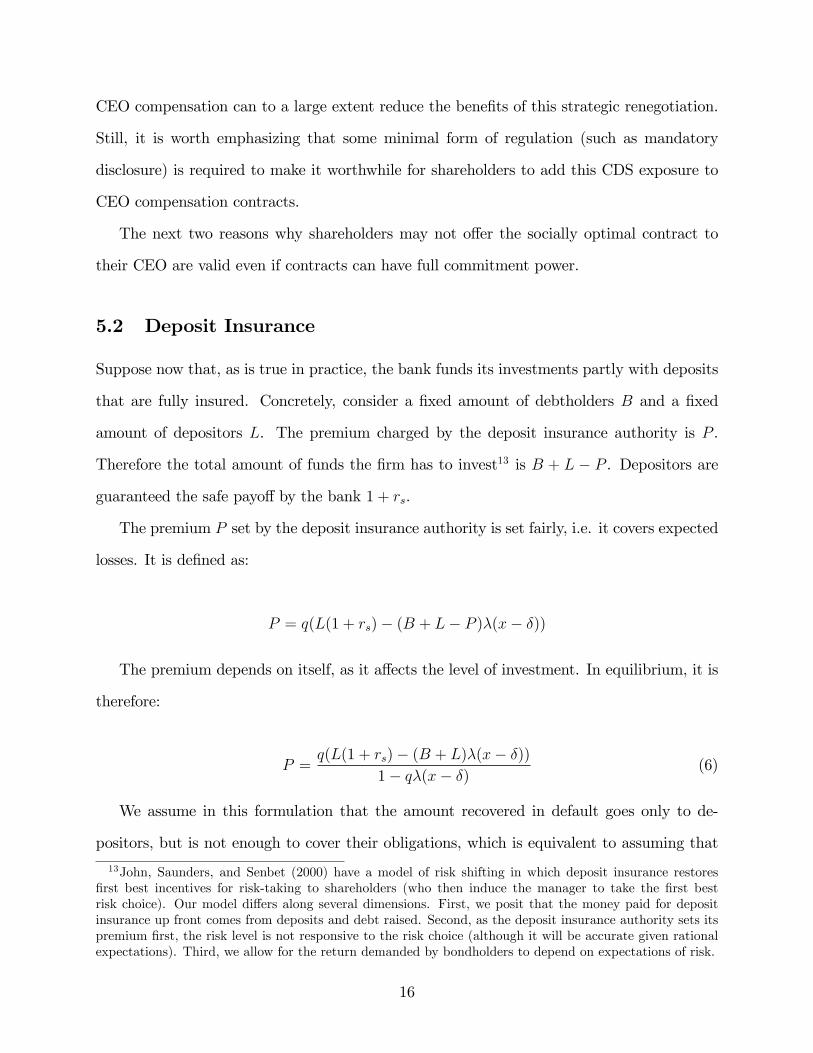
The left hand hand side of equation 3 is ∆ − x + 1 + rs when q = 0 and is increasing in q

(given A1). We depict this in Figure 2, which demonstrates that q > qo.

Using the quadratic formula on equation 3, we find that the solution exists as long as

(α + λ(x− δ) + ∆− x)2 − 4α(∆− x+ 1 + rs) > 0.

Given existence, there are actually two solutions to equation 3, both of which satisfy the

property that q > qo. Only the smaller solution, however, is stable.

Therefore, unobservable choices, although rationally expected, are riskier than observable

choices. This is because the sensitivity of debt to risk is only taken into account when the

risk choice is observable. The bank’s shareholders are worse offwith the riskier unobservable

choice. This worse outcome is due to an inability of the bank’s shareholders to commit to a

10

q

qo

αq

Δx+1+R(q)

Δx+λ(xδ)

Δx+1+rs

q

Figure 2: Excess risk taking: q > qo

lower risk exposure. We will see in the next section that under separation of ownership and

control the incentive contracting problem between the bank’s shareholders and the CEO

involves both the classical problem of aligning the shareholders’and CEO objectives and

a commitment problem with respect to the bank’s bondholders. This joint contracting

problem for a levered financial institution is an important conceptual difference with respect

to the classical moral hazard incentive contracting problem of Mirrlees (1975) and Holmstrom

(1979).

4 Separation of Ownership and Control and the choice

of unobservable risk

Suppose now that a manager decides on the level of risk. The manager’s contract, as we

stated before, is composed of three components: a fixed wage, a loading on equity as well

as a loading on the CDS spread. The equity part is standard and represents shares given

to the manager as compensation. The CDS part is the innovation. In this section we show

that it can restore optimal risk-taking incentives. In section 7, we discuss the advantages of

11

using the CDS spread over other forms of debt.

We take the price of debt to be a credit default swap (CDS) spread, which is liquid and

should reflect fundamental risk. Rather than directly sell CDSs for the manager, we envision

the firm setting aside a pool of money that can be paid out to the manager according to the

market price of the CDSs. Therefore the contract takes the following form:

Compensation = w + sEPE + sD(P − PCDS)

Since the CDS spread is increasing in the probability of default, it is judged relative to

a high benchmark P in order to align the manager’s incentives. This benchmark may come

from a weighted industry CDS spread or from a reference spread under a given risk exposure

q.

In order to analyze the optimal contract we must first define the prices. The price of

equity is given by the present discounted value of equity cash flows net of origination costs

c(q) and expected debt repayments (1− q)(1 +R(qT )). Note that in the low return state the

bank defaults and shareholders get nothing, so that the price of equity is given by:

PE = q(x+ ∆) + (1− 2q)x− (1− q)(1 +R(qT ))− 1

2αq2

Here, qT represents the risk level that bondholders believe the bank will implement

through the compensation contract.

The CDS spread, in turn, is equal to:10

q(1− λ(x− δ)1 +R(qT )

)

10More generally, if p is the CDS spread and β is the discount factor, the no-arbitrage condition is

p(1 +R(qT ))

n∑i=0

βi(1− q)i = q(1 +R(qT )− λ(x− δ))n∑i=0

βi(1− q)i

where 1 + R(qT ) is the face value and λ(x − δ) is the amount recovered in default. In our basic model,n = 0, but one can observe that if periods were added, the result would be the same.

12

where λ(x−δ)1+R(qT )

is the recovery rate of the investment.

Note that we are implicitly assuming here that the CDSs are being traded by informed

traders who observe signals that are perfectly correlated with the bank’s actual risk exposure

q, as in Holmstrom and Tirole (1993). Thus, although the bank’s actual risk choice is not

observable ex-ante when the bank issues bonds it becomes observable to analysts trading

CDS ex-post. In principle, this ex-post observability of q through the CDS price could

be incorporated into bond contracts ex-ante, but this is typically not done in practice.

Accordingly, we shall not introduce this contractual contingency into bond contracts. Note

that if we were to allow R to depend on the CDS spread we would introduce a potentially

complex fixed-point problem for the equilibrium risk choice q.

Consider first the case where the manager’s compensation package only contains stock,

so that sD = 0. Then, the manager’s objectives with respect to the choice of risk q are

perfectly aligned with shareholders’, so that the manager chooses chooses q as one would

expect and therefore takes socially excessive risk.

If instead we allow for the compensation package to be based on CDS spreads as well,

the manager maximizes his compensation by choosing q, giving us the following first order

condition:

∆− x+ (1 +R(qT ))− αq − sDsE

(1− λ(x− δ)1 +R(qT )

) = 0

Notice that the second order condition is negative.

In a rational expectations equilibrium bondholders have correct expectations about the

choice of q, so that qT = q. Using this equality, we can rewrite the first order condition as

follows:

sDsE

=∆− x+ (1 +R(qT ))− αqT

1− λ(x−δ)1+R(qT )

(4)

Can the bank implement the first best through contracting? Setting qT = qo and simpli-

13

fying, we find that:

sDsE

= 1 +R(qo) (5)

In other words, the ratio of the equity and debt loadings should be set equal to the

rate of return promised to bondholders at the optimal risk level. Although the optimal risk

level may be diffi cult to calculate, this provides a simple framework for thinking about how

to balance incentives. Moreover, opening up the black box by substituting for qo provides

further understanding:

1 +R(qo) =1 + rs − (∆−x+λ(x−δ)

α)λ(x− δ)

1− ∆−x+λ(x−δ)α

The RHS of this equation is increasing in the return on the safe investment 1 + rs.

As the need to satisfy depositors with higher returns increases and depositors themselves

are less sensitive to local change in risk, the manager will take on more risk. This is then

reined in by pushing up the loading on the CDS portion of the manager’s contract. The

expression (∆−x+λ(x−δ)) is the marginal return on a unit increase of risk. Assuming this

is positive (otherwise qo = 0), an increase in the marginal return increases the expression.

With the returns to risk-taking higher, the manager is controlled by exposing him/her to

the downside of default risk more. The term λ(x − δ) which does not represent part of

the marginal returns is the default recovery amount. The expression is decreasing in this

term. When less resources are lost to default, the need to dampen risk is lower. Lastly, the

expression is decreasing in α, the direct cost of increasing q. If it is more costly to increase

risk, there won’t need to be as much oversight through contracting incentives.

14

5 Optimal and Equilibrium CDS-based compensation

Although it is in principle possible to make use of CDS prices to induce a levered bank’s

CEO to choose a socially optimal level of risk, it is far from obvious that a levered bank’s

shareholders will make use of such incentive contracts to align the CEO’s risk-taking ob-

jectives. There are at least three reasons why we should not expect shareholders to offer

socially optimal incentive contracts to their CEOs: renegotiation, deposit insurance, and

naive bondholders.11 We explore these below.

5.1 Renegotiation

The first reason is related to the limited commitment power of contracts. As has been

pointed out in the literature on the strategic role of incentive contracts (e.g. Katz, 1991,

and Caillaud, Jullien, Picard, 1995) the optimal contract such that

sDsE

= 1 +R(qo)

may not have much commitment value if shareholders can (secretly) undo the contract once

the bonds have been issued. If that is the case, shareholders will simply offer a new contract

to the CEO after the bond issue, inducing him to change the bank’s risk exposure away from

qo.12 If that is possible, then the CDS based contract will have no value and will therefore

not be offered by shareholders. Although this issue is likely to be relevant in practice, we

have not allowed for this possibility of renegotiation and revision of the bank’s risk choice

in our model. One reason why we do not emphasize this problem is that disclosure of

11There is a fourth more subtle reason: while the shareholders prefer qo when there is no manager andwhen a manager has stock based compensation, they don’t prefer qo once there is compensation based ondebt because their objective function has changed to incorporate the fact that the wage paid is based on theCDS spread as well.12What the equilibrium risk choice is depends on how the problem is formulated. One logic is that rational

investors anticipate renegotiation and therefore pay no attention to the incentive contract in the first place.They act as if shareholders had no commitment power (as in Katz (1991)). Another logic is that they arenaive and get fooled, in which case the final outcome is like the outcome in the section on naive bondholders.

15

CEO compensation can to a large extent reduce the benefits of this strategic renegotiation.

Still, it is worth emphasizing that some minimal form of regulation (such as mandatory

disclosure) is required to make it worthwhile for shareholders to add this CDS exposure to

CEO compensation contracts.

The next two reasons why shareholders may not offer the socially optimal contract to

their CEO are valid even if contracts can have full commitment power.

5.2 Deposit Insurance

Suppose now that, as is true in practice, the bank funds its investments partly with deposits

that are fully insured. Concretely, consider a fixed amount of debtholders B and a fixed

amount of depositors L. The premium charged by the deposit insurance authority is P .

Therefore the total amount of funds the firm has to invest13 is B + L − P . Depositors are

guaranteed the safe payoff by the bank 1 + rs.

The premium P set by the deposit insurance authority is set fairly, i.e. it covers expected

losses. It is defined as:

P = q(L(1 + rs)− (B + L− P )λ(x− δ))

The premium depends on itself, as it affects the level of investment. In equilibrium, it is

therefore:

P =q(L(1 + rs)− (B + L)λ(x− δ))

1− qλ(x− δ) (6)

We assume in this formulation that the amount recovered in default goes only to de-

positors, but is not enough to cover their obligations, which is equivalent to assuming that

13John, Saunders, and Senbet (2000) have a model of risk shifting in which deposit insurance restoresfirst best incentives for risk-taking to shareholders (who then induce the manager to take the first bestrisk choice). Our model differs along several dimensions. First, we posit that the money paid for depositinsurance up front comes from deposits and debt raised. Second, as the deposit insurance authority sets itspremium first, the risk level is not responsive to the risk choice (although it will be accurate given rationalexpectations). Third, we allow for the return demanded by bondholders to depend on expectations of risk.

16

the premium is positive. Formally, it amounts to the following condition, which supersedes

assumption A1a:14

L(1 + rs)− (B + L)λ(x− δ) > 0 (A2a)

We also assume that the analogue of assumption A1b, that there will not be a default in

the middle state, is true:

x >(B + L(1− q))(1 + rs)

B + L− Lq(1 + rs)

1− qλ(x− δ)1− q (A2b)

Lastly, we assume that the total amount of funds invested B + L − P is positive for all

q, which is equivalent to:

B + L− 1

2L(1 + rs) > 0 (A3)

The expected return of debtholders depends on how much they will recover and is:

(1− q)(1 +R) ≥ 1 + rs

The timing is now:

1. Incumbent equity holders hire a manager under a linear incentive contract (w, sE, sD),

where w is the base pay, sE is the shares of equity, and sD is the loading on the credit

default swaps (CDS) of the bank.

2. The deposit insurance authority sets fees for deposit insurance.

3. The CEO chooses the probability q for the asset.

4. The bank raises B and L to fund the assets from debtholders and depositors respec-

tively, with a promised return 1 + R and 1 + rs respectively. It pays the deposit14This condition implies that both the numerator and the denominator of the premium P in equation 6

are positive (given that q ∈ [0, 12 ] and rs ∈ (0, 1)).

17

insurance fee.

5. The equity of the firm is priced at PE and the CDS spread on the firm is priced at PD.

6. The returns on the asset x are realized. Depositors and debtholders and get paid

first. In case of default, the recovery amount is distributed to depositors. The deposit

insurance authority compensates depositors for any shortfall below 1 + rs. If there are

returns left at any point, the equity holders get the residual value.

Our first benchmark is the situation where q is perfectly observed by debtholders and

the deposit insurance authority can set its fees after perfectly observing q.

In this case, the manager with a contract based on the price of equity maximizes:

maxq

(B + L− P (q)){q(x+ ∆) + (1− 2q)x− 1

2αq2}

−(1− q)(1 +R(q))B −(1− q)(1 + rs)L− P (q)

We can rewrite the problem as:

maxq

(B + L− P (q)){q(x+ ∆) + (1− 2q)x+ qλ(x− δ)− 1

2αq2} − (1 + rs)(B + L)

Not surprisingly, this expression represents total surplus. The difference with our previous

model is that P is present and depends on q.

Lemma 1 In the case where risk is observable to debtholders and the deposit insurance

authority, there is a unique optimum qoDI . Furthermore qoDI < qo.

The proof is in the appendix. The bank takes less risk when it is observable than in

the previous model because the deposit insurance premium increases with risk and therefore

reduces the bank’s returns.

18

In our second benchmark, we maintain the observability of q to debtholders, but impose

that the deposit insurance authority set its fees in advance. The bank thus takes the fee it

pays for deposit insurance as fixed, but the deposit insurance authority rationally foresees

the level of risk and sets the premium fairly. The maximization problem for the manager is

therefore:

maxq

(B + L− P (q2DI)){q(x+ ∆) + (1− 2q)x− 1

2αq2}

−(1− q)(1 +R(q))B −(1− q)(1 + rs)L− P (q2DI)

We solve and find the following result:

Lemma 2 In the case where risk is observable to debtholders but not the deposit insurance

authority, the optimum q2DI satisfies the property qoDI < qo < q2DI .

The proof is in the appendix.

The level of risk q2DI is larger than qo and qoDI . When the bank is not sensitive to the

cost it pays for deposit insurance, it increases the risk level.

Now consider the case where q is unobservable to the deposit insurance authority and

debtholders. Here, the bank takes both R(q) and deposit insurance as fixed.15 This gives us

the following objective function:

maxq

(B + L− P (qDI)){q(x+ ∆) + (1− 2q)x− 1

2αq2}

−(1− q)(1 +R(qDI))B −(1− q)(1 + rs)L− P (qDI)

This problem gives us the following result:

15Although the deposit insurance authority and the debtholders act at different times, the bank takes bothof their actions as fixed. Nevertheless we assume that both are rational and must be correct in equilibriumabout the level of risk.

19

Lemma 3 In the case where risk is unobservable to both debtholders and the deposit insur-

ance authority, the optimum qDI satisfies the property qoDI < qo < q2DI ≤ qDI .

In the appendix we demonstrate that an optimum exists, although it may not be unique.

Any solution, however, has the property that it is larger than the first benchmark qoDI and

at least as large as the second benchmark q2DI (strictly larger if the second benchmark is

an interior solution).16 This is in line with our main model - making risk unobservable to

debtholder increases the risk level the manager takes.

Using the price of debt to discipline the manager can restore the optimum of qoDI here

as well. The formula for the ratio of the share of debt to the share of equity is now more

complicated:

sDsE

= (1 +R(qoDI)− λ(x− δ))B + (1 + rs − λ(x− δ))L

+P (qoDI)λ(x− δ) +1

qoDI(1− qoDIλ(x− δ))P (qoDI)Π

where Π is value of the surplus per unit (qoDI(x + ∆) + (1 − 2qoDI)x + qoDIλ(x − δ) −12α(qoDI)2).

Importantly, without the proper incentives, shareholders will not want to implement qoDI

and implement the CDS contract. Given the friction that the deposit authority can’t observe

risk directly, it is only in the interest of shareholders to implement q2DI (if they could commit

to it), and thus take excess risk. Consequently, regulatory intervention is required in the

presence of deposit insurance to be able to implement the socially desirable level of risk. In

other words, the regulator has to step in to reduce the bank’s shareholders’ incentives to

take excess risk so as to maximize the subsidy from deposit insurance.

16This holds as long as we consider stability as the selection criteria for equilibria. This criteria is appliedin the appendix.

20

5.3 Naive debtholders

Until this point, we have considered debtholders who are completely rational. We now

suppose that they may be naive and overly optimistic. By naive, we mean that debtholders

do not consider the incentives of the CEO regarding risk. By optimistic, we mean that

debtholders expect the risk level to be equal to the optimal level qo. For a CEO whose

contract does not have the debt component, the maximization problem is then:

maxq

q(x+ ∆) + (1− 2q)x− (1− q)(1 +R(qo))− 1

2αq2

with the first order condition:

∆− x+ (1 +R(qo)) = αq (7)

From figure 1, it should be clear that the solution to equation 7, qN , has the property that

it is larger than the optimal risk (qN > qo). Therefore, naivete encourages risk taking. At the

same time, the risk level is lower than the amount a manager would take when debtholders

are rational but risk is unobservable (qN < q). From a social surplus perspective, it is thus

better to have the naive debtholders than rational ones when q is unobservable.

This logic only goes so far. From the perspective of shareholders and the CEO this

increases returns. However, the increase in returns comes from two sources - an increase in

actual expected returns, and a transfer of expected returns from debtholders to shareholders.

Debtholders expect (incorrectly) that their returns will be equal to 1 + rs, when in fact their

expected returns will be less because of risk taking by the manager. So although returns are

higher, debtholders are worse off in this scenario.

Can this be corrected by the modification in the compensation package proposed in the

previous subsection? The answer is yes, and in fact, the solution is identical to before,

sDsE

= 1 + R(qo). This is simple to see from the derivation of the rule for rational investors.

Again, however, it is not in shareholders’interest to implement such a correction. Regulatory

21

intervention is required to achieve this reduction in risk taking.

What about bondholders who are naive, but pessimistic? Consider, for example, bond-

holders who do not take into account the manager’s incentives, but expect risk to be high,

say q. In this case, the bondholders’beliefs are self-fulfilling. Switching qo to q in equation 7

and comparing to equation 3 demonstrates that the risk level chosen by the CEO will be q.

The CEO thus takes more risk here than when debtholders are optimistic. Overall returns

are down, and the amount expropriated from an individual debtholder is zero, as he gets an

expected return of 1 + rs. The debtholder protects herself with the low expectations of the

manager’s performance, but increases risk taking.

In order to mitigate this risk taking, a contract based on debt can be implemented here as

well, although the rule would be slightly different. The ratio of the shares of debt to equity

will be larger to take into account the excess risk, sDsE

= 1 +R(q). Regulatory intervention is

also required here to implement this lower level of risk.

6 Leverage

Suppose the CEO now has to raise funds and that the number of debtholders and hence the

amount of debt to hold is no longer fixed. What is the effect of leverage on risk taking? We

will assume that the project returns exhibit decreasing returns to scale - the more debt, the

lower the expected returns.17 Specifically, for an amount of debt I ∈ [0, I] we make the loss

in case of default δ an increasing and convex function of I. One way to think about these

decreasing returns are that as more projects default, it becomes more diffi cult to process and

recover value, as in the case for mortgages and foreclosures in the recent crisis.

Our benchmark here is the scenario where both q and I are observable and the bank

takes into account the opportunity cost of debtholders. The bank maximizes:

17We will assume the project cost is still constant returns to scale, however.

22

maxI,q

I{q(x+ ∆) + (1− 2q)x− (1 + rs − qλ(x− δ(I)))− 1

2αq2}

The first order condition with respect to q yields a similar result to before:

qoL =∆− x+ λ(x− δ(I))

α

Note that the optimal level of risk is decreasing in leverage.

The first order condition with respect to I is:

{q(x+ ∆) + (1− 2q)x− (1 + rs − qλ(x− δ(I)))− 1

2αq2} = Iqλδ′(I)

We will call the optimal level of leverage IoL.

Now consider the case where both q and I are unobservable. The bank maximizes:

maxI,q

I{q(x+ ∆) + (1− 2q)x− (1− q)(1 +R(qL, IL))− 1

2αq2}

The bank’s choice of leverage now does not affect the cost of debt. This implies that for

positive equity prices, the bank chooses the maximum amount of leverage I. How much risk

does the bank take for this amount of leverage? The first order condition is the analogue of

equation 3:

∆− x+1 + rs − qLλ(x− δ(I))

1− qL = αqL

Assuming that a solution exists as in Figure 1, we observe that risk is increasing in

leverage (qL is increasing in I).18 More leverage decreases the size of the assets recovered in

default, meaning that the bank has to pay out more when not defaulting, encouraging it to

take more risk.18The left hand side of the equation is increasing in I, holding q fixed. In figure 1, we can see that this

moves the curve upward, so the stable solution increases.

23

Will linking compensation to the price of debt reduce risk and leverage? We now show

that we can restore the first best. First, notice that the CDS spread is increasing with

leverage:

PCDS = q(1− λ(x− δ(I))

1 +R(qTL, ITL))

The manager maximizes:

maxI,q

[sEI{q(x+ ∆) + (1− 2q)x− (1− q)(1 +R(qTL, ITL))− 1

2αq2} −

sDq(1−λ(x− δ(I))

1 +R(qTL, ITL))]

Which yields the following first order conditions:

q : ITL{∆− x+ (1 +R(qTL, ITL))− αqTL − sDsE

(1− λ(x− δ)1 +R(qTL, ITL)

) = 0

I : {qTL(x+ ∆) + (1− 2qTL)x−

(1 + rs − qTLλ(x− δ(ITL)))− 1

2α(qTL)2} − sD

sE

qTLλδ′(ITL)

1 +R(qTL, ITL)= 0

It is straightforward to demonstrate that the solution is the analogue of the one in the

main model:

sDsE

= IoL(1 +R(qoL, IoL))

7 Empirical Analysis

Although our model is normative and proposes modifying compensation in a new way, this

section offers evidence suggesting that linking pay to credit quality is likely to produce results

supporting the paper’s thesis. We focus on the recent disclosure of deferred compensation

24

and pension benefits in proxy statements filed with the SEC. Below, we discuss our data and

our methodology.

7.1 Data

Enhancing transparency of managers’ deferred compensation holdings and pension bene-

fits was a key feature of the Securities and Exchange Commission’s expansion of executive

compensation disclosure at the end of 2006. We use this information to study CDS investor

reactions to disclosure of CEO deferred compensation and pension benefits at listed financial

institutions that reported compensation to shareholders in 2007.

Specifically, we focus on banking firms. We collected deferred compensation and pensions

as well as equity compensation from proxy filings in EDGAR. CEO pension benefits may

sometimes be negotiated, but they usually accrue to managers under company-wide formulas

established by each company. Deferred compensation is generally paid out to the executive

at retirement. We collected additional data from COMPUSTAT and CRSP for calculating

the Black-Scholes stock option values as well as the value of CEO equity holdings. Lastly,

we required banks in our sample to have CDS quotes data from Markit, our data source

for daily CDS spreads.The spreads are for five-year, senior unsecured CDS with a "Modified

Restructuring" clause, which was usually embedded in a firm’s most widely traded contract

before 2009. To enter the final sample, a bank must have CDS daily quotes on the disclosure

day (event day 0) and the subsequent trading day (event day 1). Overall, this sampling

procedure gives us 27 banks for our final sample.

7.2 Methodology

We follow a methodology similar to that of Wei and Yermack (2011) to produce a CDS

event study of the first-time disclosure of deferred compensation and pensions in banks.19

19Wei and Yermack (2011) study non-financial firms and find that the revelation of more CEO inside debtincreases debt prices, decreases equity prices, and lowers the CDS spread for non-financial firms. Sundaramand Yermack (2007) find a significant positive effect of inside debt on the distance to default measure for a

25

In a standard event study, security returns (equity or bond) are analyzed to estimate the

unexpected component (abnormal return) in the returns within a window surrounding the

event. The abnormal return (AR) on the event day is calculated by adjusting the return to

exclude changes due to market movement. Both AR and the cumulative abnormal return

(CAR) through several days surrounding the event provide an assessment of the event’s

impact on the security value. In the CDS market, however, spread is the main valuation

metric. To follow the standard approach as closely as possible, we use daily percentage

changes of CDS spread in the event analysis. Specifically, the daily “spread”return (SR) for

firm i on day t, is calculated as

SR(i, t) =[Spread(i, t)− Spread(i, t− 1)]

Spread(i, t− 1)(8)

To control for the market movement, we next define the market “spread”return (SRm) as

the equally weighted average of daily CDS spreads for all financial firms20 (with n denoting

the total number of firms).

SRm(t) =

∑ni=1 SR(i, t)

n(9)

To calculate daily abnormal “spread”returns (ASR), we deduct the CDS market spread

return from the individual CDS spread return on each day t.

ASR(i, t) = SR(i, t)− SRm(t) (10)

Lastly, the cumulated abnormal “spread”return (CASR) between event day 0 and day

1 is calculated as the sum of ASR on event day 0 and 1. CASR is the key measure used in

the cross-section analysis as reported in Table 2.

sample of 237 of the Fortune 500 firms from 1996-2002.20The total number of financial firms is 125.

26

CASR(i) = ASR(i, 0) + ASR(i, 1) (11)

7.3 Results

Table 1 presents CEO total wealth, which is the sum of the value of stock holdings, options

and restricted stock holdings, pensions, and deferred compensation. On average, a bank

CEO’s wealth is about $287 million (with a median of $95 million). The average value of

CEO equity holdings is about $265 million (with a median of $61 million). Bank CEOs

have nearly $10 million in pensions and another $10 million in deferred compensation (with

medians of nearly $5 million and $6 million in deferred bay and pensions, respectively).

The percentage of CEOs’total wealth in deferred pay and pensions is about 7% and 11%,

respectively. On average, the ratio of a bank CEOs’ sum of deferred compensation and

pensions to their equity holdings is 26% (median of 29%), with the ratio of deferred pay to

equity holdings of 10% (median of 7%) and pension to equity holdings of 16% (median of

14%).

Ratios of deferred pay and pensions to total wealth or equity holdings are critical in

our analysis. We expect more CEO conservatism the higher these ratios are. Wei and

Yermack (2011) and Edmans and Liu (2010) argue that both deferred pay and pensions are

unsecured in the event of default. As a result, CEOs with large holdings in deferred pay and

pensions are unlikely to undertake risky investment choices. If available, the information

on both deferred pay and pensions can prove helpful to credit market analysts. Firms were

first required to disclose this information in their proxy filings in the beginning of 2007.

Therefore, we anticipate that the credit market reacted to the news in proxy filings since

disclosure began.

We estimate announcement credit market CDS spreads over the window of (0,1) for the

27 banks with actively traded CDS. The announcement returns by themselves are not very

informative as proxy fillings contain other information as well. We perform a cross-sectional

27

test of the returns and the results are reported in Table 2. It should be noted that in

our OLS estimates, we do not control for firm-specific characteristics. The main reason

is that we have only 27 banks and consequently few degrees of freedom in our analysis.

However, this may not be relevant for the following reasons. First, we are using a highly

homogeneous industry. All the banks are very large. Furthermore, the average (median)

book debt to assets ratio in these large banks is about 92%. Also, these banks arguably face

similar investment opportunity sets, and as Smith and Watts (1992) have pointed out, the

investment opportunity set drives other corporate polices.

We estimate four models21 which are presented in Table 2. In model (1), we estimate

the effect of the ratio of the sum of deferred pay and pensions to equity holdings on CDS cu-

mulative abnormal returns. The coeffi cient is negative and significant, suggesting that firms

with a higher investment in deferred compensation and pensions experience a larger reduc-

tion in their credit spreads. In model (2), we estimate the effect of deferred compensation

and pensions separately. However, the estimates are not significant. In model (3), we create

a (0,1) dummy for the ratio of the sum of deferred compensation and pensions to equity

holdings. The dummy takes the value 1 whenever the firm’s ratio is above the median value

of the ratio in the sample (29%). We find that firms with an investment in deferred pay and

pensions relative to equity holdings above the median, experience a lower credit spread at

the proxy announcement. We create two more dummies separately for the ratios of deferred

pay to equity holdings and pensions to equity holdings, equal to 1 for observations above the

median of the sample (7% and 14%, respectively), and these estimates are reported in model

(4). We find firms with higher than median investment in deferred compensation experience

2.6% larger reduction in their CDS spreads net of market movements relative to firms below

21Wei and Yermack (2011) also use a slightly different independent variable, which was suggested by thework of Edmans and Liu (2010): they normalize the inside debt and equity holdings of the CEO by the debtand equity levels of the firm. With this variable, our results are qualitatively similar, but less significant.The reason is that all bank CEO personal leverage ratios are below the corresponding bank leverage ratiosbecause of the typically high leverage in banks. Moreover, deposit insurance and too-big-to-fail concernsmake it unclear what ratio we should use to capture the “risky”debt part of bank liabilities.

28

the median investment. The high pension dummy is not significant, however.

Overall, we find some results suggesting that the disclosure of deferred compensation

and pension benefits is priced in credit markets. Firms with larger investments in CEO

deferred compensation experience a reduction in the CDS spreads at proxy announcements.

A plausible reason for this reduction may be that banks are likely to be more conservative

in terms of the riskiness of their investment choices.

8 Why not use other debt-based compensation?

Our model demonstrates the effi cacy of CDS-based compensation in reducing risk taking.

In the model, other debt-like instruments (including debt itself) would reduce risk taking as

well. This raises the natural question of why the focus should be on CDS-based compensation

rather than on other instruments tied to debt. In this section we address this question

directly. We begin by demonstrating that CDS-based compensation will be less costly to use

than deferred compensation. We then discuss the practical diffi culties of including debt in

compensation rather than basing it on the CDS spread.

8.1 Deferred Compensation

Deferred compensation is a debt-like instrument since it is unsecured and hence its payoff

depends on the probability of default. In this subsection, we slightly extend the model to

demonstrate that deferred compensation is not as effective as using CDS based compensation.

The model is extended in a very natural way. Previously, the CEO implicitly consumed his

wage subsequent to the market pricing the firm’s financial instruments. Now, we allow for

two periods (t = 1, 2) of consumption for the CEO and introduce a discount factor β. The

first period is subsequent to market pricing but before the realization of the state. The

second period follows the realization of the state.

Consider first a CEO receiving only deferred equity compensation, i.e. all of the com-

29

pensation is in equity and is deferred until t = 2. In the current model, the CEO would still

choose the excessively high risk level of q. Moreover, to provide a fixed consumption target

level (e.g. if the participation constraint of the CEO were made to bind), the firm would

have to compensate the CEO with more equity than if the equity compensation were not

deferred. This would make shareholders even more resistent to adopting such a scheme, and

potentially cause more distortion.

Next, consider deferred cash compensation C given in addition to (non-deferred) equity

compensation. Assuming linear utility for the CEO, the CEO maximizes:

maxqscashE PE + β(1− q)C

It is important to note that giving cash that can be consumed at period t = 1 would not

affect risk taking at all. The key here is that it is deferred, so the CEO will lose it if the

low state occurs. While in reality the CEO may not lose all of her deferred cash in the low

state (this depends on negotiations with other creditors) as we have assumed here, partial

loss will not make a difference for the qualitative results.

Using the results of the maximization problem, the optimal level of risk taking qo can be

achieved by setting the equity weighting and cash levels such that:

C

scashE

=1 + rs − λ(x− δ)

β(1− qo)

The CEO therefore consumes:

scashE PE(qo) + β(1− qo)C(qo)

which when simplifying is:

scashE (PE(qo) + 1 + rs − λ(x− δ))

30

The consumption of the CEO when CDS-based compensation is given is:

sCDSE PE(qo) + sD(P − PCDS(qo))

Since P is a free parameter, we can set it equal to PCDS(qo), implying that consumption

for the CEO is simply sCDSE PE(qo). Assuming that the CEO has a binding participation

constraint with outside option U , the equity weights scashE and sCDSE are pinned down, and

the CEO is indifferent between the two schemes. The firm, however, may not be indifferent

between the two schemes. Firstly, if the firm must set aside the cash upfront, it is paying

more than the CEO is receiving in consumption value due to discounting. Second, since cash

may be strictly more expensive for a firm than granting equity22, the cost to the firm of the

CEO’s compensation is larger with deferred compensation than CDS-based compensation.23

Notice that the CDS-based compensation can be implemented by cash (rather than giving

the CEO CDS contracts), but it ends up being very low cost (or costless if we set P perfectly).

It is also interesting to point out that deferred CDS-compensation would work equally well

as upfront CDS compensation in this model.

8.2 Debt

In our model, we focus on the use of CDS spreads as the tool to moderate risk taking

incentives. We specifically use CDS based compensation because it is market based and can

be chosen optimally. Several other methods of compensation have been proposed that rely

on other debt instruments. We view theses as helpful but subject to practical problems of

implementation. Specifically, the practical problems lie in the structuring and valuation of

the debt, as well as in its tax treatment.

Structuring and Valuation —Depending on the type of debt used, it may be diffi cult

22One reason would be tax benefits, as in Babenko and Tserlukevich (2009).23This in some sense a thought exercise, as we have shown earlier that shareholders would not implement

q0 given their commitment problem. This implies they prefer not to have either CDS-based or deferredcompensation to correct risk taking incentives. If they were offered a choice, we demonstrate that CDS-based compensation is cheaper for them.

31

and/or costly to value the debt instrument at issuance and on an on-going basis. Individual

debt issues vary by maturity, seniority, and specific covenants, while the CDS spread does

not. Actual debt credit spreads may reflect liquidity and taxes (see Longstaff, Mithal, and

Neis (2005)) and may lag CDS spreads (see Norden and Weber (2009), Blanco, Brennan,

and Marsh (2005), Forte and Peña (2009)). As credit default swaps become even more

standardized and liquid by being moved onto exchanges, their benefits may be magnified.

Other key issues are deciding on the maturity of the debt (employees may prefer shorter

maturity rather than be exposed to interest rate risk, while the bank may prefer longer

maturity) and its seniority. It is also unclear how rating agencies would view this debt in

their overall credit analysis. On top of this, it is not known whether regulators would treat

employee-held debt as regulatory capital.

Tax issues —First, paying an employee in debt is a compensation contract as well as a

debt contract and is diffi cult to design and manage given human resources guidelines and

the Federal tax laws and employment laws. Careful analysis is needed to determine whether

the deductibility of wage payments from corporate taxation can be made equivalent to the

deductibility of interest payments. Second, would debt be treated as ordinary income to an

employee, and how would vesting work? Does the employee have income on day 1 equal to

the principal amount of the debt awarded to the employee, without having the ability to sell

a portion of the debt to cover his/her tax liability (i.e., phantom income)? If so, this could

effectively erode a portion of the employee’s cash compensation for the year (in the amount

of the additional tax liability).

9 Implementation of CDS-based compensation

Concretely, how should bank CEO compensation be tied to CDS spreads in practice? One

way may be to require that CEOs write a given amount of CDS (or buy swaps written

by other insurers) for the duration of their employment contract. Alternatively and more

32

effi ciently, using money set aside by the bank, their deferred bonuses may be reduced under

a pre-specified formula as the bank’s CDS spread deviates from the average bank spread24:

bonuses would be increased if the spread is below average and decreased if it is above average.

A potential argument against tying bonuses to CDS spreads is that CDS spreads were not

immediately responsive to the deterioration of bank capital during the crisis. For example,

the average market value of equity to assets of 18 large institutions that participated in

the U.S. SCAP program started to decline in Q4 2006 but the CDS spreads (on average)

only began to react in Q2 2007.25 Firstly, linking payments to an average CDS diminishes

this issue26. Secondly, despite the onset of the crisis, major financial institutions initiated

oversized bonus payments in 2008 and 2009. Public pressure forced banks to forgo paying

a large fraction of their contractual bonuses.27 Meanwhile, in the period from Q2 2007 to

Q2 2008, the eighteen firm average CDS spread increased from about 20 to 280 basis points,

and to 308 at the end of Q1 2009. Using our approach of tying bonuses to the CDS spread

surely could have prevented the firms from initiating bonus payouts (without regulatory

intervention or public pressure). Thirdly, one side-benefit of our approach is that it creates a

built-in stabilizer using compensation that would have been useful in the crisis. When banks’

performance deteriorates and their credit quality weakens (and they experience an increase

in their CDS spread), the banks will be forced to conserve capital through the automatic

adjustment of bonuses. Our approach is thus in a sense analogous to cutting dividends to

protect the bank and its creditors. While cutting dividends imposes a cost on all equity

holders, our approach imposes a direct cost on risk-taking managers as well.

24In the section on deferred compensation, we suggest another possible benchmark: the CDS spreadevaluated at the optimal level of risk. In this case, in expectation there would be zero cost for the bank.25This can be seen in Figure 4 in Flannery (2010).26In the section comparing CDS spreads with debtlike instruments, we suggest that deferred pay such

as debt will be costly. We also point out that deferred CDS may be less costly, depending on where thebenchmark is set.27Arguably, banks would have been unable to pay the bonuses in the absence of government support during

the crisis (such as the TARP capital infusion).

33

10 Conclusion

In this paper we propose using a recent innovation in financial markets, the credit default

swap, to reduce risk taking of executives at highly levered financial firms. The CDS provides

a market price for risk, which, when weighted correctly in a compensation contract that

includes an equity component, can provide first best risk incentives. We demonstrate that

while in their interest, shareholders would be reluctant to adopt this type of contract due

to a commitment problem that may be exacerbated by renegotiation, deposit insurance,

and/or naive debtholders. We provide evidence that the market believes that including

debtlike instruments in CEO compensation packages will reduce risk. While other debtlike

instruments are available, basing compensation on the CDS spread is likely to be (i) cheaper,

because it does not need to be deferred and (ii) easier to implement, because it is relatively

more liquid.

34

References

[1] Adams, R. B and H. Mehran, (2003). “Is Corporate Governance Different for Bank

Holding Companies?,”Federal Reserve Bank of New York Economic Policy Review, 9

(1), 123-142.

[2] Babenko, I. and Y. Tserlukevich, (2009). “Analyzing the Tax Benefits from Employee

Stock Options", Journal of Finance, 64, 1797-1825.

[3] Balachandran, S., B. Kogut, and H. Harnal (2010). “The Probability of Default, Ex-

cessive Risk, and Executive Compensation: A Study of Financial Services Firms from

1995 to 2008”, Columbia Business School Discussion Paper

[4] Bebchuk, Lucian A., and Holger Spamann (2010). “Regulating Bankers Pay”, George-

town Law Journal, 98(2), 247-287.

[5] Blanco, R., Brennan, S., and I.W. Marsh (2005) “An Empirical Analysis of the Dy-

namic Relation between Investment-Grade Bonds and Credit Default Swaps”, Journal

of Finance, 60, 2255—2281.

[6] Brander, James A., and Michel Poitevin, 1992, “Managerial compensation and the

agency costs of debt finance”, Managerial and Decision Economics 13, 55-64.

[7] Caillaud, B., B. Jullien, and P. Picard. (1995). “Competing Vertical Structures: Pre-

commitment and Renegotiation.”Econometrica, 63, 621—46.

[8] Chesney, M., Stromberg, J., Wagner, A. (2010) “Risk-Taking Incentives, Governance,

and Losses in the Financial Crisis,”Research Paper 10-18, Swiss Finance Institute.

[9] DeFusco, R. A., R. R. Johnson, and T. S. Zorn. (1990) “The Effect of Executive Stock

Option Plans on Stockholders and Bondholders”, Journal of Finance 45:617-627.

[10] DeYoung, R., Peng, E.Y. and M. Yan (2009) “Executive compensation and business

policy choices at U.S. commercial banks”, Mimeo.

35

[11] Edmans, A., and Q. Liu (2010). "Inside Debt", Review of Finance, 1—28.

[12] Ellul, A. and V. Yerramilli (2010) “Stronger Risk Controls, Lower Risk: Evidence from

U.S. Bank Holding Companies”, mimeo, Indiana University.

[13] Flannery, M. (2010). “What to do about TBTF?”, Univseristy of Florida, mimeo.

[14] Forte, S. and J.I. Peña (2009), “Credit spreads: An empirical analysis on the informa-

tional content of stocks, bonds, and CDS”, Journal of Banking & Finance, 33, 2013-

2025.

[15] Green, R.C. (1984). “Investment Incentives, Debt, and Warrants”, Journal of Financial

Economics, 13, 115-136.

[16] Greenlaw, D., Kashyap, A.K., Schoenholtz, K., and H.S. Shin (2011), “Stressed Out:

Macroprudential Principles for Stress Testing”, mimeo, Princeton University.

[17] Hart, O. and L. Zingales (2010), “Curbing Risk on Wall Steet”, National Affairs, 20-34.

[18] Holmstrom, B. (1979) “Moral Hazard and Observability.” The Bell Journal of Eco-

nomics, 10:1, 74-91.

[19] Holmström, B., and J. Tirole (1993). “Market Liquidity and Performance Monitoring.”

Journal of Political Economy, 101, 678—709.

[20] Jensen, M. C., and W. H. Meckling (1976). “Theory of the Firm: Managerial Behavior,

Agency Costs and Ownership Structure.”Journal of Financial Economics, 3, 305—60.

[21] Jensen, M. C., and K. J. Murphy (1990). “Performance Pay and Top-Management

Incentives”, Journal of Political Economy, 98, 225—264.

[22] John, T. A. and K. John, 1993, “Top-Management Compensation and Capital Struc-

ture,”Journal of Finance, Vol. XLVIII, No.3, 949-74.

36

[23] John, K., Mehran, H. and Y. Qian, 2010, “Regulation, Subordinated Debt and Incen-

tive Features of CEO Compensation in the Banking Industry”, Journal of Corporate

Finance, forthcoming.

[24] John, K., A. Saunders, and L. Senbet, 2000, “A Theory of Bank Regulation and Man-

agement Compensation,”Review of Financial Studies 13, no. 1: 95-125.

[25] Katz, M. L. (1991). “Game-Playing Agents: Unobservable Contracts as Precommit-

ments.”Rand Journal of Economics, 22(3).

[26] Levine, R. (2004). “The Corporate Governance of Banks: A Concise Discussion of

Concepts and Evidence”, World Bank Policy Research Working Paper 3404.

[27] Longstaff, F.A., Mithal, S., and E. Neis (2005), “Corporate Yield Spreads: Default Risk

or Liquidity? New Evidence from the Credit Default Swap Market”Journal of Finance,

60, 2213—2253.

[28] Macey, J., and M. O’Hara. (2003) “The Corporate Governance of Banks.”Federal Re-

serve Bank of New York Economic Policy Review, 9:1, 91-107.

[29] Mehran, H. and J. Rosenberg (2008). “The effect of employee stock options on bank

investment choice, borrowing, and capital.”Federal Reserve Bank of New York Staff

Report 305.

[30] Mehran, H., Morrison, A., and J. Shapiro (2011). “Corporate Governance and Banks:

What Have We Learned From the Financial Crisis?”mimeo, Federal Reserve Bank of

New York.

[31] Mirrlees, J. A. (1975) “The Theory of Moral Hazard and Unobservable Behaviour: Part

I.”reprinted in Review of Economic Studies (1999) 66, 3-21.

[32] Norden, L. and M. Weber (2009), “The Co-movement of Credit Default Swap, Bond and

Stock Markets: an Empirical Analysis”, European Financial Management, 15, 529-562.

37

[33] Smith, Clifford, and Ross Watts (1992). “The investment opportunity set and corporate

financing, dividend, and compensation policies.”Journal of Financial Economics, 33,

263-292.

[34] Sundaram, R.K., and D.L. Yermack (2007) “Pay Me Later: Inside Debt and Its Role in

Managerial Compensation”, Journal of Finance, 62, 1551—1588.

[35] Wei, Chenyang, and David Yermack (2011). “Deferred Compensation, Risk, and Com-

pany Value: Investor Reaction to CEO Incentives.”Review of Financial Studies, forth-

coming.

A Appendix

A.1 Proof of Lemma 1

Taking the first order condition of the objective function yields:

0 = −P ′(q){q(x+ ∆) + (1− 2q)x+ qλ(x− δ)− 1

2αq2}+ (12)

(B + L− P (q)){∆− x+ λ(x− δ)− αq}

First note that P ′(q) = 1q(1−qλ(x−δ))P (q) > 0. We will assume that q(x+∆)+(1−2q)x+

qλ(x − δ) − 12αq2 > 0 for all q ∈ [0, 1

2], which says the project has positive NPV for all q.

This then implies, from equation 12, that for any solution, ∆− x+ λ(x− δ)− αq > 0.

Taking the derivative of the FOC, we get:

−P ′′(q){q(x+ ∆) + (1− 2q)x+ qλ(x− δ)− 1

2αq2}

−2P ′(q){∆− x+ λ(x− δ)− αq} − α(B + L− P (q))

38

The expression P ′′(q) = 2qλ(x−δ)q2(1−qλ(x−δ))2P (q) > 0. Assumption A3 ensures that B + L −

P (q) > 0. As we noted above, the FOC implies that ∆−x+λ(x−δ)−αqoDI > 0. Remember

that qo from our original model satisfied the condtion ∆ − x + λ(x − δ) − αqo = 0. This

implies that qoDI < qo. Furthermore, it implies the objective function is strictly concave

over the interval [0, qo]. It may not be concave over the interval [qo, 12], but as there is no

inflection point in that interval, meaning that qoDI must be the global maximum.


Taking the first order condition of the objective function and then setting q = q2DI yields:

0 = (B + L− P (q2DI)){∆− x− αq2DI}+ (1 + rs)L (13)

Rewriting this equation, we get:

B + L− P (q2DI) =(1 + rs)L

αq2DI − (∆− x)(14)

First, examine the left hand side. At q2DI = 0, it is equal to B + L. As we showed in

Lemma 1, it is decreasing and concave, and assumption A3 assures it is positive.

Next, examine the right hand side and for now, take ∆−xα

< 12. When q2DI < ∆−x

α,

the right hand side is negative, decreasing, concave, and approaching negative infinity as

q2DI approaches ∆−xα

−. When q2DI > ∆−x

α, the right hand side is positive, decreasing, and

concave (and approaching positive infinity as q2DI approaches ∆−xα

+). Therefore the right

hand side may intersect the left hand side when q2DI > ∆−xα0,1, or 2 times. If it does not

intersect, that implies the solution is for the manager to choose the maximum q2DI = 12as the

first order condition in equation 13 is positive holding fixed the deposit insurance authority

expectations at q2DI = 12. If it intersects twice, both intersections are rational expectations

equilibria, but only the smaller one is stable.

If ∆−xα

> 12, the solution would be q2DI = 1

2.

39

Now we prove that qoDI < qo < q2DI . Clearly, this must be the case if q2DI = 12.

Otherwise, we can rewrite equation 13 by adding and subtracting λ(x−δ)(B+L−P (q2DI)):

0 = (B +L− P (q2DI)){∆− x+ λ(x− δ)− αq2DI}+ (1 + rs)L− λ(x− δ)(B +L− P (q2DI))

Simplifying, we get:

0 = (B + L− P (q2DI)){∆− x+ λ(x− δ)− αq2DI}+1

qP (q2DI)

This implies that ∆− x+ λ(x− δ)− αq2DI < 0, which proves our statement.


The first order condition of the problem is (we also set q = qDI):

0 = (B + L− P (qDI)){∆− x− αqDI}+ (1 + rs)(B

1− qDI + L) (15)

We proceed with a similar approach to Lemma 2.

Rewriting the FOC, we get:

B + L− P (qDI) =(1 + rs)(

B1−qDI + L)

αqDI − (∆− x)(16)

First, examine the left hand side. At q2DI = 0, it is equal to B + L. As we showed in

Lemma 2, it is decreasing and concave, and assumption A3 assures it is positive.

Next, examine the right hand side and take ∆−xα

< 12. When qDI < ∆−x

α, it is negative

and approaching negative infinity as qDI approaches ∆−xα

−. When qDI > ∆−x

α, it is positive

(and coming from positive infinity as qDI approaches ∆−xα

+). Furthermore, for any qDI such

that qDI > ∆−xα, the right hand side is strictly larger than the right hand side in equation

14. Therefore if there are zero intersections for equation 14, there are zero for the current

40

equation and qDI = 12. If there is one intersection for equation 14, then the solution qDI is

strictly larger than q2DI and may be equal to 12.28 If there are two intersections for equation

14, than the solution qDI is strictly larger than the stable rational expectations equilibria

q2DI .

If ∆−xα

> 12, the solution would be q2DI = 1

2.

28There may be multiple solutions here, but all will be larger than q2DI .

41

Table 1: Summary Statistics of CEO Compensation Disclosed in Proxy Statements for the

27 banks with CDS spreads

Total wealth is the sum of the value of stock holdings, option holdings, deferred compensation,

and pension balance. Stock holdings are valued by multiplying the number of shares times the

stock price at the end of 2006. The figure includes restricted and performance shares. Options are

valued by the number of options times the Black-Scholes value of each option using data from

Compustat and CRSP. Equity is the sum of the value of stock holdings and option holdings.

Deferred compensation, equity holdings, and pension balance are from proxy statements filed

with the SEC.

Variable Obs. Mean Median StandardDeviation

Minimum Maximum

Total Wealth ($MM) 27 287.26 95.24 839.37 27.57 4463.64

Value of Stock Holdings ($MM) 27 230.81 39.87 837.14 11.34 4407.67

Value of Option Holdings ($MM) 27 35.13 21.59 30.83 0 96.69

Deferred Compensation ($MM) 27 10.70 4.82 17.71 0 86.12

Pension Balance ($MM) 27 10.61 6.14 11.77 0 49.15

Deferred Compensation / TotalWealth

27 0.07 0.06 0.08 0 0.28

Pension Balance / Total Wealth 27 0.11 0.11 0.10 0 0.27

Deferred Comp + Pensions / Equity 27 0.26 0.29 0.22 0 0.64

Deferred Comp / Equity 27 0.10 0.07 0.12 0 0.44

Pension / Equity 27 0.16 0.14 0.14 0 0.41

Table 2: Cross-Section Regression of Cumulative CDS Abnormal Spread Changes on Newly Disclosed

CEO Compensation

Dependent variable: cumulative CDS abnormal spread changes between the day of disclosure (event date 0) and

the subsequent trading day (event date 1). The CDS contracts are five-year, senior unsecured CDS with a

"Modified Restructuring" clause and spreads are collected from Markit. Total wealth is the sum of the value of

stock holdings, option holdings, deferred compensation, and pension balance. Stock holdings are valued by

multiplying the number of shares times the stock price at the end of 2006. The figure includes restricted and

performance shares. Options are valued by the number of options times the Black-Scholes value of each option

using data from Compustat and CRSP. Equity is the sum of the value of stock holdings and option holdings.

Deferred compensation, equity holdings, and pension balance are from proxy statements filed with the SEC.

High indicates above the median value for the sample.

(1) (2) (3) (4)

Constant 0.016*(1.83)

0.016(1.69)

0.011(1.16)

0.021**(2.49)

Pension + Deferred Comp / Equity -0.055**

(2.77)

Deferred Comp / Equity -0.058

(1.36)

Pension / Equity -0.052

(1.14)

High (Pension + Deferred Comp) / Equity -0.021*

(1.90)High Deferred Comp / Equity -0.026*

(1.84)

High Pension / Equity -0.018

(1.34)

Observations 27 27 27 27

r-squared 13% 13% 11% 33%

Robust t statistics in parentheses: * significant at 10% ** significant at 5% *** significant at 1%

Documents

Executive Compensation and Risk Taking