Executive Compensation-Implied CEO Risk-Taking and Systemic Risk

of Bank Holding Companies

G. Nathan Dong 1 Columbia University

May 27th, 2018

ABSTRACT

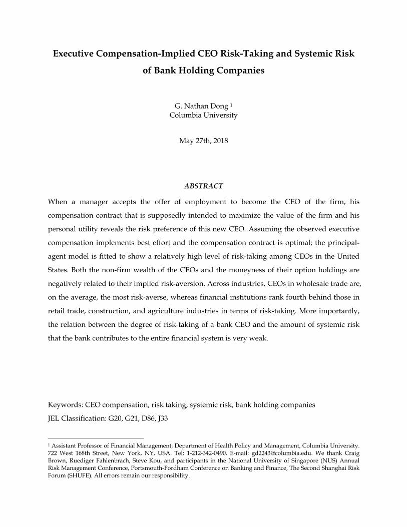
When a manager accepts the offer of employment to become the CEO of the firm, his

compensation contract that is supposedly intended to maximize the value of the firm and his

personal utility reveals the risk preference of this new CEO. Assuming the observed executive

compensation implements best effort and the compensation contract is optimal; the principal-

agent model is fitted to show a relatively high level of risk-taking among CEOs in the United

States. Both the non-firm wealth of the CEOs and the moneyness of their option holdings are

negatively related to their implied risk-aversion. Across industries, CEOs in wholesale trade are,

on the average, the most risk-averse, whereas financial institutions rank fourth behind those in

retail trade, construction, and agriculture industries in terms of risk-taking. More importantly,

the relation between the degree of risk-taking of a bank CEO and the amount of systemic risk

that the bank contributes to the entire financial system is very weak.

Keywords: CEO compensation, risk taking, systemic risk, bank holding companies

JEL Classification: G20, G21, D86, J33

1 Assistant Professor of Financial Management, Department of Health Policy and Management, Columbia University. 722 West 168th Street, New York, NY, USA. Tel: 1-212-342-0490. E-mail: gd2243@columbia.edu. We thank Craig Brown, Ruediger Fahlenbrach, Steve Kou, and participants in the National University of Singapore (NUS) Annual Risk Management Conference, Portsmouth-Fordham Conference on Banking and Finance, The Second Shanghai Risk Forum (SHUFE). All errors remain our responsibility.

2

“In recent years, anti-regulatory ideology kept the United States from modernizing the rules of the capitalist game in a period of intense financial innovation and perverse incentives to creep in.”

― Alice Rivlin’s Testimony before the House Committee on Financial Service, July 21, 20092

“Shareholders’ interest in more risk-taking implies that they could benefit from providing executives with excessive incentives in this direction. Executives with such incentives can use their informational advantages, and whatever discretion they have been left by existing regulations, to increase risks.”

― Financial Times, August 3, 20093

I. Introduction

Despite a large body of studies on estimating the distribution of individuals’ risk preferences in

various settings, prior literature of inferring the degree of risk aversion (or concavity of

marginal utility) of decision makers such as corporate executives is scarce, and little research

has been done to examine the link between an executive’s risk preference and the characteristics

of both the manager and the company. Senior executives play a critical role in not only

formulating business strategy and ensuring operational efficiency but also answering for

financial performance to the shareholders. Understanding the heterogeneity of their risk

preferences is important in order to link risk-taking incentives embedded in executive

compensation contracts to managerial and strategic decisions, such as altering capital structure,

hoarding cash, allocating capital investments, manipulating accounting numbers, and

committing financial fraud. Therefore, the question of whether senior executives of publicly

traded companies exhibit high or low degree of risk aversion becomes a relevant concern and

has not been conclusively resolved. More importantly, in the banking sector, financial

innovations such as securitization with which bank assets (mainly mortgages) can be easily sold

to other investors offer financial services firms the advantage of reduced cost of asset sales that

eventually causes higher levels of risky lending (Santomero and Trester 1998). The public anger

over the executive compensation at financial firms–coupled with common beliefs that

compensation-induced excessive risk-taking was the root cause of the 2008-10 financial crisis

(see the quotes above 4)–led to the question of whether top executives of financial services firms

2 Excerpt from Rivlin (2009). 3 Except from Bebchuk (2009). 4 For the detailed discussion of this issue in EU countries, see Murphy (2013).

3

actually responded to compensation incentives to take excessive risks that eventually led to the

crisis.

The main challenge to answer this question lies in the fact that it is difficult, if not

possible, to quantify or measure risk preferences of corporate executives in a laboratory setting.

Even a controlled experiment is conducted it is very likely that their risky choice in the lab

situation does not resemble the decision-making behavior they might display in the real-world

business environment. In this paper, we propose a calibration method to recover risk-aversion

measures of corporate executives from their observed compensation contracts. It is well known

that individuals with different degrees of risk aversion choose different types of contracts

(Ackerberg and Botticini 2002; Allen and Lueck 1995). In the context of executive compensation

design, the decision that a manager serves as CEO of the firm and receives compensation in the

form of stock and options is materially affected by the interaction of risk preference and

compensation structure (e.g., cash salary, stock and options). On the one hand, CEOs with a

certain level of risk-aversion choose to work for firms offering compensation contracts with

embedded risk profiles that match those of CEOs, and on the other hand, holding executive

stock and options may increase or decrease managerial risk taking, as illustrated theoretically

by Ross (2004) and empirically by Lewellen (2006), among others. In equilibrium, the

compensation contract maximizes the firm value and the CEO’s utility, and the observed

contract implements the CEO’s optimal action. Therefore, fitting the standard principal-agent

model using observed executive compensation contracts can reveal the CEOs’ risk preferences.

This research contributes to existing evidence on estimating the implied risk aversion

and relating the degree of risk-taking of bank CEOs to the level of systemic risk (i.e., the amount

of risk that each individual bank contributes to the entire financial system). There is a

voluminous literature on option-implied risk preferences, surveyed by Bliss and Panigirtzoglou

(2002). For example, risk preferences can be estimated by applying the semi-parametric method

of Aït-Sahalia and Lo (1998, 2000) for estimation of the option-implied density function in two

steps. The first step estimates implied strike prices from the deltas as a smooth function,

following Bliss and Panigirtzoglou (2004) and Kang and Kim (2006), and the second step plugs

the GBS volatility function in a lognormal density. As a final step, the Aït-Sahalia and Lo

estimator yields relative risk aversion and marginal rate of substitution, both depending on the

stock price. However, this type of estimation method only produces firm-level risk preference,

4

and unfortunately, it offers little help in understanding the degree of risk-aversion on the CEO

level. These issues are in focus after the introduction of accounting standards IFRS 2 (see

International Accounting Standards Board, 2004), SAB 107, and FAS 123R (see Securities and

Exchange Commission, 2005), and the Dodd-Frank Wall Street Reform and Consumer

Protection Act (see Securities and Exchange Commission, 2015), requiring publicly traded firms

to expense the value of executive stock options and to disclose the ratio of the CEO

compensation to the median compensation of its employees. In contrast to common practice,

this paper extends the principal-agent models of Holmstrom (1979), Dittmann and Maug (2007),

and Armstrong, Larcker and Su (2007) and calibrate the model with observed cash salary, stock

and options in executive compensation contracts to estimate the risk-aversion of individual

CEOs. As the first paper to address the question if executive compensation contributed to the

financial crisis, Fahlenbrach and Stulz (2011) find no evidence that banks with CEOs whose

incentives were better aligned with the interests of their shareholders performed better during

the crisis. Also evidence indicates that these banks actually performed worse. Banks whose

CEOs had better incentives in terms of the dollar value of their stake in the company performed

significantly worse than banks where CEOs had poorer incentives. This implies that incentive

compensation had no adverse impact on bank performance during the crisis. While many of the

bank CEOs made high cost, bad bets that cost themselves and their shareholders, the data

suggests that CEOs took these bets because they believed they would be profitable for the

shareholders. On the contrary, Bennett, Guntay and Unal (2012) show that banks with CEOs

holding more inside-debt relative to equity in 2006, experienced higher default risk and lower

stock returns in 2008.

The closest paper to our risk-aversion estimation approach is Brenner (2015), who

estimates the risk preferences of U.S. executives from data on the exercising of employee stock

options. Its calibration method makes use of the assumption that these senior corporate

managers (as option holders) choose the stock prices at which to exercise the options such as to

maximize their subjective value. Such approach has the advantage of relying on a simplistic

argument over the optimal choice of the share price that triggers the option exercise to identify

the risk preferences, while our approach requires a condition of “optional contract”, meaning

the executive would only be offered a contract of employment to serve as the CEO of the firm if

the compensation reflected the optimal level of efforts that the CEO-elect would exert in order

5

to maximize the firm value. Nonetheless, our calibration result of the average Arrow-Pratt

measure of relative risk-aversion being 4.6 for 290 long-serving CEOs in the United States, to

some extent, is consistent with the finding in Brenner (2015) that senior executives are more risk

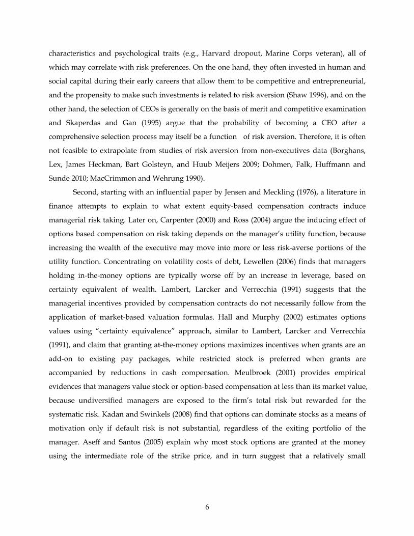
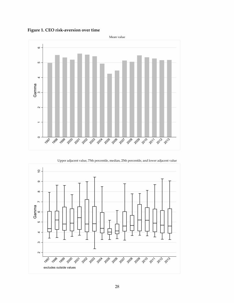
taking than managers of lower rank. What is more interesting in our study is that the mean

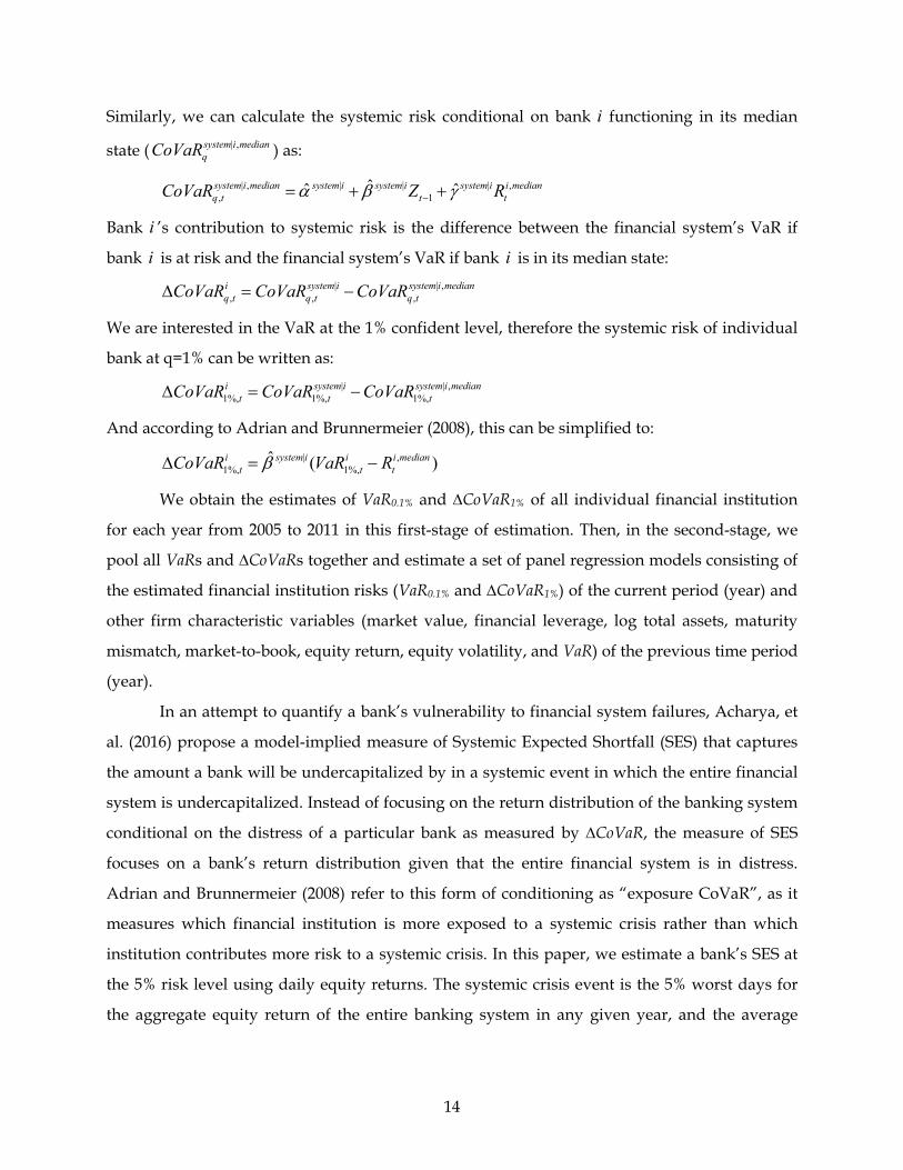
level of risk aversion of American CEOs remains stable (between 4.2 to 5.5) over a long period

of time from 1997 to 2013, as shown in Figure 1, except a slight fluctuation between 2004 and

2006. However, the box plot of upper adjacent value, 75th percentile, median, 25th percentile,

and lower adjacent values presents a slightly different picture: the distribution changes

dramatically over time and since 2001, the median level of risk-aversion has been gradually

declining, with some fluctuations, and reached the lowest level in 2005 and 2006 before

bouncing back again in 2007 and 2008. To some extent, this evidence may support the argument

that excessive risk-taking was a major contributing factor of the recent financial crisis of 2008-

2010, at least on the aggregate; however, when we actually use two measures of systemic risk

that proxy for the amount of risk that an individual bank contribute to the entire financial

system (SES and CoVaR),5 the relationship between bank CEO risk-aversion and systemic risk

vanishes.

[Insert Figure 1 Here]

The remainder of the paper is organized as follows. Section II reviews the relevant prior

research. Section III specifies the theoretical model and empirical method in detail. Section IV

describes the sample data. Section V presents empirical results. Section VI discusses the

implication and concludes.

II. Related Literature

This paper is related to four strands of literature. The first set of related studies provide some

evidence on the risk preferences of executives, for example, Grahama, Harvey and Puri (2013)

for privately held firms. In a more recent study, Cain and McKeon (2016) use the possession of a

FAA (Federal Aviation Administration) pilot license and living near a major airport to identify

risk-seekers among executives and find that risk-seeking pilot CEOs engage in more

acquisitions that eventually lead to positive value creation. Corporate senior executives

represent a demographic group that is often associated with a very special set of socioeconomic

5 SES (Acharya et al. 2016) in and CoVaR (Adrian and Brunnermeier 2016).

6

characteristics and psychological traits (e.g., Harvard dropout, Marine Corps veteran), all of

which may correlate with risk preferences. On the one hand, they often invested in human and

social capital during their early careers that allow them to be competitive and entrepreneurial,

and the propensity to make such investments is related to risk aversion (Shaw 1996), and on the

other hand, the selection of CEOs is generally on the basis of merit and competitive examination

and Skaperdas and Gan (1995) argue that the probability of becoming a CEO after a

comprehensive selection process may itself be a function of risk aversion. Therefore, it is often

not feasible to extrapolate from studies of risk aversion from non-executives data (Borghans,

Lex, James Heckman, Bart Golsteyn, and Huub Meijers 2009; Dohmen, Falk, Huffmann and

Sunde 2010; MacCrimmon and Wehrung 1990).

Second, starting with an influential paper by Jensen and Meckling (1976), a literature in

finance attempts to explain to what extent equity-based compensation contracts induce

managerial risk taking. Later on, Carpenter (2000) and Ross (2004) argue the inducing effect of

options based compensation on risk taking depends on the manager’s utility function, because

increasing the wealth of the executive may move into more or less risk-averse portions of the

utility function. Concentrating on volatility costs of debt, Lewellen (2006) finds that managers

holding in-the-money options are typically worse off by an increase in leverage, based on

certainty equivalent of wealth. Lambert, Larcker and Verrecchia (1991) suggests that the

managerial incentives provided by compensation contracts do not necessarily follow from the

application of market-based valuation formulas. Hall and Murphy (2002) estimates options

values using “certainty equivalence” approach, similar to Lambert, Larcker and Verrecchia

(1991), and claim that granting at-the-money options maximizes incentives when grants are an

add-on to existing pay packages, while restricted stock is preferred when grants are

accompanied by reductions in cash compensation. Meulbroek (2001) provides empirical

evidences that managers value stock or option-based compensation at less than its market value,

because undiversified managers are exposed to the firm’s total risk but rewarded for the

systematic risk. Kadan and Swinkels (2008) find that options can dominate stocks as a means of

motivation only if default risk is not substantial, regardless of the exiting portfolio of the

manager. Aseff and Santos (2005) explain why most stock options are granted at the money

using the intermediate role of the strike price, and in turn suggest that a relatively small

7

additional cost to the principal in compensation such as the use of simple stock options can

incentivize the agent to exert high effort.

A third related literature use calibration technique of option pricing models, such as by

eliciting subjective option values from calibrating utility models to observed exercise pattern by

employees (e.g., Ingersoll 2006; Bettis, Bizjak and Lemmon 2005). A small subset of these studies

ask if the observed compensation contract reflects the optimal level of the CEO’s effort, we can

actually find another contract, with a new mix of salary, stock and options, which will cost less

to the firm. In a typical principal-agent model, to maximize financial returns, the principal has

to incentivize the agent to exert the optimal level of effort and in turn take the appropriate

amount of risk (Holmstrom and Milgrom 1987). However, the difficulty to find an optimal

managerial compensation contract lies in the fact that we cannot quantify the optimal level of

the CEO’s effort. Dittmann and Maug (2007) assume the observed compensation contracts

implement the optimal action, meaning the beginning stock price anticipates the optimal effort

that will be selected by the agent for a given compensation contract. This assumption simplifies

the classical principal-agent problem to a principal-only problem. Their model predicts that

optimal compensation schemes should have no or at best miniscule holdings of stock options,

and incentives should be provided through restricted stock. Finally, Armstrong, Larcker and Su

(2007) avoid the use of first order approach as in Dittmann and Maug (2007) and reach the exact

opposite conclusion that stock options are an important part of the optimal CEO compensation

contact.

Most of these papers do not calibrate a principal-agent model explicitly to back out

the CEO’s managerial risk aversion. This paper takes a step further and proposes a new

numerical calibration approach to back out the degree of managerial risk preference by

assuming not only the optimal effort but also the optimal contract, meaning that the observed

executive compensation has already attained the level at the lowest cost to the firm. In previous

studies, Hall and Murphy (2000) and Hall and Murphy (2002) use assumed risk aversion

coefficients, because empirical estimates are few and exhibit significant variation. This paper

contributes to the literature by estimating relative risk-aversion based on executive

compensation data including cash-based salary, stock and options.

Of course, this paper is also closely related to the literature on systemic risk. The

contagion effect of an event usually refers to the spillover effects of stocks of one or more firms

8

to others (Kaufman 1994), but has also been characterized as the change in the value of a firm

that can be attributed to economic events with a clearer and more direct impact on some other

firm (Docking, Scott, Hirschey, and Jones 1997). Contagion has been studied widely in the

theoretical and empirical financial literature (for reviews see Flannery 1998). The focus of

analysis has ranged from strong systemic shocks involving multiple bank failures, currency

crises, and market crashes to informational spillover effects that lead to the revaluation of stock

prices but not to widespread failures. This paper contributes to this body of literature by

connecting a bank CEO’s risk-taking propensity to the amount of risk that a bank contributes to

the stability of the entire financial system. To do so we we use the CoVaR measure developed

by Adrian and Brunnermeier (2016) and the Systemic Expected Shortfall (SES) measure in

Acharya et al. (2016) to measure systemic risk.

III. Numerical and Empirical Methods

We assume that the traditional moral hazard model is an appropriate representation of the

contracting problem involving principal and agent. My model is based on a traditional single

period agency setting with a risk-neutral principal (i.e., the representative shareholder in theory

and the board of directors in reality) and a risk-averse and effort-averse agent (i.e., the CEO).

The CEO has an additively separable utility function (CRRA) defined over terminal wealth, the

sum of the initial wealth compounded at risk-free rate in one period and the current period

compensation:

1

( )1T

T

WU W

, γ ≠ 1

( ) ln( )T TU W W , γ = 1

The CEO’s disutility of the effort, D(e), is a convex and monotonic increasing function of

effort e. The CEO selects the effort level to maximize the expected utility of terminal wealth less

the disutility. It is assumed that CEO’s choice of effort satisfy the incentive compatibility (IC)

constraint.

The risk-neutral principal selects a compensation contract to maximize the expected

value of the firm net of the expected compensation to the CEO. We assume that the

compensation contains only cash (salary and bonus), restricted stock and stock options, and the

principal decides the allocation of the compensation among these types. We require the

9

minimum payment (MP) constraint or limited liability, meaning the cash compensation is

greater than or equal to zero. This is consistent with Armstrong, Larcker and Su (2007). It is not

a trivial constraint, and it has serious impact on the result of this non-linear optimization

problem that we. Dittmann and Maug (2007) allow cash compensation bounded below at CEO’s

negative initial wealth: 0W . Their result has negative cash compensation and zero weight

in options, and they in turn argue for all restricted stock grants as optimal compensation.

Without the limited liability constraint, the CEOs are forced to invest all their wealth to their

company stocks. This is like replicating stock options in discrete time using delta number of

stocks.

The no-shorting (NS) constraint is that the number of stock and the number of options

are positive and the total shares (TS) constraint is that the total number of stocks and options is

less than total shares outstanding. It is further assumed that the compensation satisfies the

individual rationality (IR) constraint that the expected utility from this compensation contract

less the cost of effort is greater than or equal to the utility of the reservation wage that the CEO

can earn in the outside the executive labor market.

The basic principal’s problem is defined as follows. The principal (shareholders)

maximizes expected profit, measured as total market value of equity net of compensation paid

to the agent (CEO) subject to incentive compatibility (IC) and participation constraint (IR):

1 21 2

, , ,[ ( max( ,0)) | ]T T T

eMax E NP P P K e

s.t. 0 1 2arg max{ [ (( ) max( ,0)) | ] ( )}fr T

T Te

e E U W e P P K e D e

(IC)

0 1 2[ (( ) max( ,0)) | ] ( )fr T

T TE U W e P P K e D e U (IR)

0 (MP)

1 20, 0 (NS)

1 2 N (TS)

N is the total number of shares outstanding. α is the cash compensation including salary

and bonus. β1 is the number of restricted stocks granted to the CEO. β2 is the number of stock

options granted to the CEO with strike price K. W0 is CEO’s initial wealth. D(e) is the CEO’s

disutility of action or effort, e, and U is the CEO’s reservation utility. PT is the terminal stock

price at time 1, and its distribution is lognormal: 2

( )2

0

fr T u T

TP P e

, where (0,1)u N .

10

Without any assumption of disutility function D(e), the implementation of the model depends

on first-order approach which replaces the (IC) constraint with the respective first-order

condition for utility maximization by the CEO, by assuming observed compensation contracts

imply optimal actions of CEOs. Following the definition of utility-adjusted pay-for-performance

sensitivity in Dittmann and Maug (2007):

0 1 2( ) max( ,0)fr T

T T TW W e P P K

The first order condition of the IC constraint: arg max{ [ ( ) ( )}Te

e E U W D e

is:

0

0

( ) ( )[ ] 0T dPdU W dU dD eE

de dP de de

UPPS is defined as:

0 0

0 0

( ) ( )( )[ ] [ ]f fr T r TT TT

TT

dW P dW PdU WUPPS e E e E W

dW dP dP

UPPS depends only on the observable compensation contract parameters including WT

and γ, but not P0(e) and D(e). We further assume that the observed compensation contracts

reflect the optimal action taken by that CEO, thus UPPS can be inferred from the observed

contract data. In addition to this “optimal effort” condition, the model assumes that the

observed pay structure (i.e., the allocation of executive compensation in the form of salary, stock

and options) has already attained the level at the lowest cost to the firm. The degree of risk-

aversion (Gamma or γ) can be implied by numerically solving the following optimization

problem. The level of risk-aversion (γ) at which the principal (shareholders) minimizes the cost

of executive compensation subject to incentive compatibility of the agent’s choice of effort (IC)

and participation constraint (IR) that the agent’s expected net utility from the contract is at least

as great as his outside option.

1 0 2 0Min P C

s.t. 1 2 1, 2,( ( , , )) ( ( , , ))T T observed observed observedUPPS W UPPS W (IC)

1 2 1, 2,[ ( ( , , ))] [ ( ( , , ))]T T observed observed observedE U W E U W (IR)

observed , 1 1,observed , 2 2,observed

P0 is the stock price at time 0, and C0 is the call options price estimated by the Black-Scholes

formula.

11

The object function is linear; however there is a non-linear constraint, namely the UPPS

function. We use the estimation method in Dong (2014) to solve this non-linear programming

problem. Basically, the solver applies a sequential quadratic programming (SQP) method which

solves a quadratic programming (QP) sub-problem at each iteration, then updates an estimate

of the Hessian of the Lagrangian at each iteration using the BFGS formula. Internally, the solver

performs a line search using a merit function and the QP sub-problem is solved using the

active-set strategy. There is an additional constraint for the optimization that the value of

gamma is within the range of 0 to 10. This restriction is based on the findings in prior studies

that the degree of risk-aversion is generally smaller than 10 (Arrow 1971; Friend and Blume

1975; Hansen and Singleton 1982, 1984; Epstein and Zin 1991; Ferson and Constantinides 1991;

Jorion and Giovannini 1993; Normandin and St-Amour 1998; Ait-Sahalia and Lo 2000; Guo and

Whitelaw 2006). Unfortunately, when this constraint is strictly enforced as in the first half of the

tests in this paper, many firm-CEO pairs may not have feasible solutions. Because we suspect

that this restriction is too strong to be of much use, we will relax it to be within the range of 0 to

20 in the second half of the tests that relate bank CEO risk-taking to systemic risk.

After obtaining the implied risk-aversion (Gamma or γ) of individual CEOs, we conduct

pooled OLS regression in the following form to study the cross-sectional variation of

managerial risk preference in terms of CEO characteristics (e.g., age, non-firm wealth),

compensation contract characteristics (e.g., salary, stock grants, option grants, stock ownership

and option ownership) and firm financial characteristics (e.g., asset size, financial leverage,

market to book, asset turnover, return on equity, stock return, cash liquidity):

, 0 1 , 2 , 3 , ,i t i t i t i t i tGamma CEO Chars Compensation Chars FirmChars

In order to capture systemic risk in the financial sector we use two econometric

measures: ∆CoVaR (Adrian and Brunnermeier 2016) and SES (Acharya et al. 2016). ∆CoVaR is

the value at risk of the entire financial system conditional on an individual institution in distress.

More formally, ∆CoVaR is the difference between the CoVaR, conditional on a financial

institution being in distress, and the CoVaR, conditional on its operating in its median state. A

number of papers have used the ∆CoVaR measure in various contexts. Brunnermeier, Dong, and

Palia (2012) find that banks actively engaged in trading, investment banking and venture capital

contributed more to systemic risk and Gauthier, Lehar and Souissi (2012) use it to examine

Canadian institutions. Adrian and Brunnermeier (2008) suggest that prudential capital

12

regulation should not just be based on the Value-at-Risk (VaR) of a bank but also on the ∆CoVaR,

which by their predictive power alert regulators who can use them as a basis for a preemptive

countercyclical capital regulation such as a capital surcharge or Pigovian tax.6

Let |system iqCoVaR denote the Value at Risk of the entire financial system (portfolio)

conditional on bank i being in distress (in other words, the loss of bank i is at its level of iqVaR ).

That is, |system iqCoVaR is essentially a measure of systemic risk in the q% quantile of this

conditional probability distribution:

|( | )system system i i iq qProbability R CoVaR R VaR q

Similarly, let | ,system i medianqCoVaR denote the financial system’s VaR, conditional on a bank

operating in its median state (in other words, the return of bank i is at its median level). That is,

| ,system i medianqCoVaR measures the systemic risk when business is normal for bank i :

| ,( | )system system i median i iqProbability R CoVaR R median q

Bank i ’s contribution to systemic risk can be defined as the difference between the

financial system’s VaR conditional on bank i in distress ( |system iqCoVaR ), and the financial

system’s VaR conditional on bank i functioning in its median state ( | ,system i medianqCoVaR ):

| | ,i system i system i medianq q qCoVaR CoVaR CoVaR

To estimate this measure of an individual bank’s systemic risk contribution, i.e., iqCoVaR , we

need to calculate two conditional VaRs for each bank, namely |system iqCoVaR and

| ,system i medianqCoVaR . For the systemic risk conditional on a bank being in distress ( |system i

qCoVaR ),

we run a 1% quantile regression using the weekly data 7 to estimate the coefficients i , i ,

|system i , |system i and |system i :

1i i i it tR Z

6 For detailed discussions of financial institution risk, see Dong and Calluzzo (2015). 7 It should be noted that for each financial institution on average there are three observations for the dependent variable that are in the 1% quantile region given that we have six years of weekly data: 52×6×0.01=3.12. Similarly, we have this data scarcity issue in estimating 0.1% VAR. This problem of data scarcity occurs when the sample size is not very large and the estimated quantile is low (0.1% and 1%) relative to the size of the data, and the problem is made worse by the presence of control variables and fixed effects. We will address this concern using alternative estimation methods in the robustness check section.

13

| | | |1 1

system system i system i system i i system it t tR Z R

and run a 50% quantile (median) regression to estimate the coefficients ,i median and ,i median :

, , ,1

i i median i median i mediant tR Z

where itR is the weekly market-value return of bank i at time t and system

tR is the weekly

market-value return of all N banks ( 1,2,3...,i j N ) in the financial system at time t . 1tZ is

the vector of macroeconomic and finance factors in the previous week, including market return,

equity volatility, liquidity risk, interest rate risk, term structure, default risk and real-estate

return. We obtain value-weighted market returns from the database of the S&P 500 Index CRSP

Indices Daily. We use weekly value-weighted equity returns (excluding ADRs) with all

distributions to proxy for the market return. Volatility is defined as the standard deviation of

log market returns. Liquidity risk is defined as the difference between the three-month LIBOR

rate and the three-month T-bill rate. For the next three interest rate variables we calculate the

changes from this week t to t-1. Interest rate risk is defined as the change in the three-month T-

bill rate. Term structure is defined as the change in the slope of the yield curve (yield spread

between the 10-year T-bond rate and the three-month T-bill rate. Default risk is defined as the

change in the credit spread between the 10-year BAA corporate bonds and the 10-year T-Bond

rate. All interest rate data is obtained from the U.S. Federal Reserve website and Compustat

Daily Treasury database. Real estate returns are proxied by the Federal Housing Finance

Agency’s FHFA House Price Index for all 50 U.S. states.

We predict an individual bank’s VaR and median equity return using the coefficients ˆ i ,

ˆ i , ,ˆ i median and ,ˆ i median estimated from the quantile regressions:

, 1ˆˆ ˆi i i i

q t t tVaR R Z

, , ,1

ˆˆ ˆi median i i median i mediant t tR R Z

After obtaining the unconditional VaRs of an individual bank i ( ,iq tVaR ) and that bank’s asset

return in its median state ( ,i mediantR ), we predict the systemic risk conditional on bank i being in

distress ( |system iqCoVaR ) using the coefficients |ˆ system i , |ˆ system i , and |ˆ system i estimated from this

quantile regression:

| | | |, 1 ,

ˆˆ ˆ ˆsystem i system system i system i system i iq t t t q tCoVaR R Z VaR

14

Similarly, we can calculate the systemic risk conditional on bank i functioning in its median

state ( | ,system i medianqCoVaR ) as:

| , | | | ,, 1

ˆˆ ˆsystem i median system i system i system i i medianq t t tCoVaR Z R

Bank i ’s contribution to systemic risk is the difference between the financial system’s VaR if

bank i is at risk and the financial system’s VaR if bank i is in its median state:

| | ,, , ,i system i system i medianq t q t q tCoVaR CoVaR CoVaR

We are interested in the VaR at the 1% confident level, therefore the systemic risk of individual

bank at q=1% can be written as:

| | ,1%, 1%, 1%,i system i system i mediant t tCoVaR CoVaR CoVaR

And according to Adrian and Brunnermeier (2008), this can be simplified to:

| ,1%, 1%,

ˆ ( )i system i i i mediant t tCoVaR VaR R

We obtain the estimates of VaR0.1% and ∆CoVaR1% of all individual financial institution

for each year from 2005 to 2011 in this first-stage of estimation. Then, in the second-stage, we

pool all VaRs and ∆CoVaRs together and estimate a set of panel regression models consisting of

the estimated financial institution risks (VaR0.1% and ∆CoVaR1%) of the current period (year) and

other firm characteristic variables (market value, financial leverage, log total assets, maturity

mismatch, market-to-book, equity return, equity volatility, and VaR) of the previous time period

(year).

In an attempt to quantify a bank’s vulnerability to financial system failures, Acharya, et

al. (2016) propose a model-implied measure of Systemic Expected Shortfall (SES) that captures

the amount a bank will be undercapitalized by in a systemic event in which the entire financial

system is undercapitalized. Instead of focusing on the return distribution of the banking system

conditional on the distress of a particular bank as measured by ∆CoVaR, the measure of SES

focuses on a bank’s return distribution given that the entire financial system is in distress.

Adrian and Brunnermeier (2008) refer to this form of conditioning as “exposure CoVaR”, as it

measures which financial institution is more exposed to a systemic crisis rather than which

institution contributes more risk to a systemic crisis. In this paper, we estimate a bank’s SES at

the 5% risk level using daily equity returns. The systemic crisis event is the 5% worst days for

the aggregate equity return of the entire banking system in any given year, and the average

15

equity return of a bank during these “worst” market days is defined as this bank’s SES at the 5%

level.

After obtaining both the implied risk-aversion (Gamma or γ) of individual CEOs and the

measures of systemic risk (∆CoVaR and SES) of individual bank holding companies, we conduct

pooled OLS regression in the following form to study the cross-sectional variation of

managerial risk preference in terms of CEO characteristics (e.g., age, non-firm wealth),

compensation contract characteristics (e.g., salary, stock grants, option grants, stock ownership

and option ownership) and firm financial characteristics (e.g., asset size, financial leverage,

market to book, liquidity, loan portfolio, etc.):

, 0 1 , 2 , 3 , ,i t i t i t i t i tSystemic Risk CEO Chars Compensation Chars FirmChars

In addition, to mitigate the omitted variable problem (i.e., unobserved CEO and firm

characteristics), we include firm fixed-effects to exploit the variation over time in our measures

of CEO risk-aversion as reflected by the risk-taking incentives embedded in the executive

compensation contract.

IV. Sample Data

The sample consists of 290 CEOs from the Compustat Executive Compensation database during

the period of 2003 to 2013. This rather small sample size reflects the requirement that these

executives have been serving as CEOs for ten years, meaning their compensation contract

information must exist in the Executive Compensation database for at least ten consecutive

years. The wealth of a CEO is calculated by taking the present value of their 10-year cash pays

including salaries and bonuses plus a 15-year annuity equal to 60% of CEO’s cash compensation.

This estimation is based on the method used by Armstrong, Larcker and Su (2007). The values

of stock price and return, dividend yield, common shares outstanding are taken from the CRSP

database, firm level financial accounting information is from the Compustat Annual database,

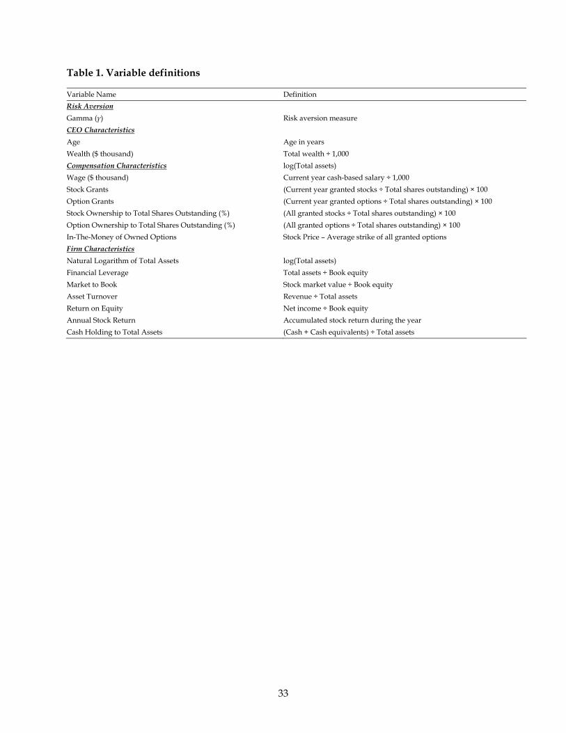
and the annual risk-free rate is downloaded from the U.S. Treasury web site. Table 1 shows the

detailed definition of all variables used in this research.

[Insert Table 1 Here]

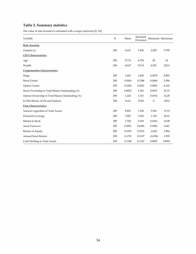
We require sample data have non-zero values of salary, stock and option holdings,

shares outstanding, stock price, Black-Scholes value, volatility, and total compensation in each

16

year. Table 2 shows the number of observations, mean, standard deviation, maximum and

minimum values of each variable.

[Insert Table 2 Here]

The average CEO in the sample is 58 years old with $40 million wealth as a result of

accumulating his cash compensation during the previous ten years of employment. The average

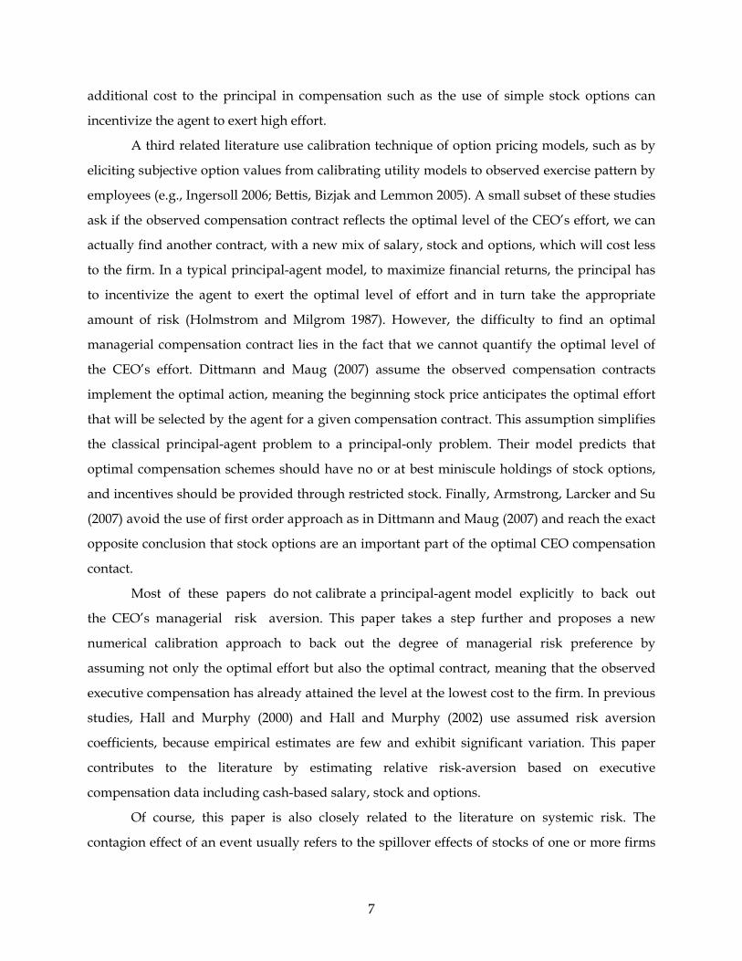
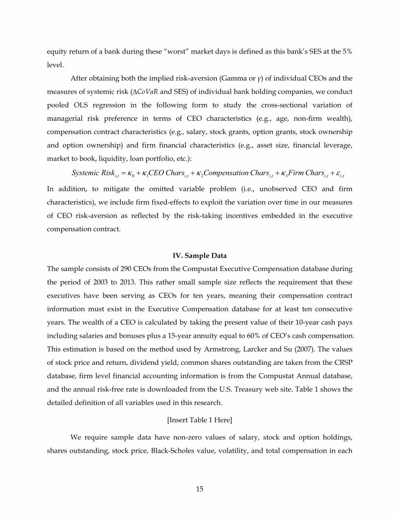
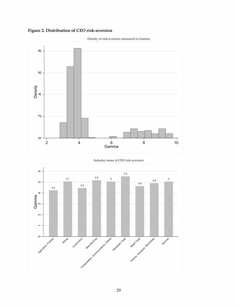
degree of risk aversion implied by the numerical method proposed in this paper is 4.6, and its

distribution (probability density) and industry means of this Arrow-Pratt measure of relative

risk-aversion are shown in Figure 2. The majority of CEOs, more than half of the sample, are

clustered at a lower level of risk-aversion with mean below 4.0 and the others are clustered at a

higher level of risk-aversion between 7.0 and 9.0. It is interesting to note that chief executives in

wholesale trade industry (5.5) are, on the average, the most risk-averse of all nine industry

groups, followed by those in manufacture and mining industries. CEOs in finance, insurance

and real estate industries (4.9) rank fourth behind those in retail trade, construction, and

agriculture industries in terms of risk-taking.

[Insert Figure 2 Here]

It is important to note that the value of Gamma is within the range of 0 to 10 due to a constraint

that is enforced in the optimization estimation. This restriction is based on the findings in prior

studies that the degree of risk-aversion is generally smaller than 10, and we will relax this

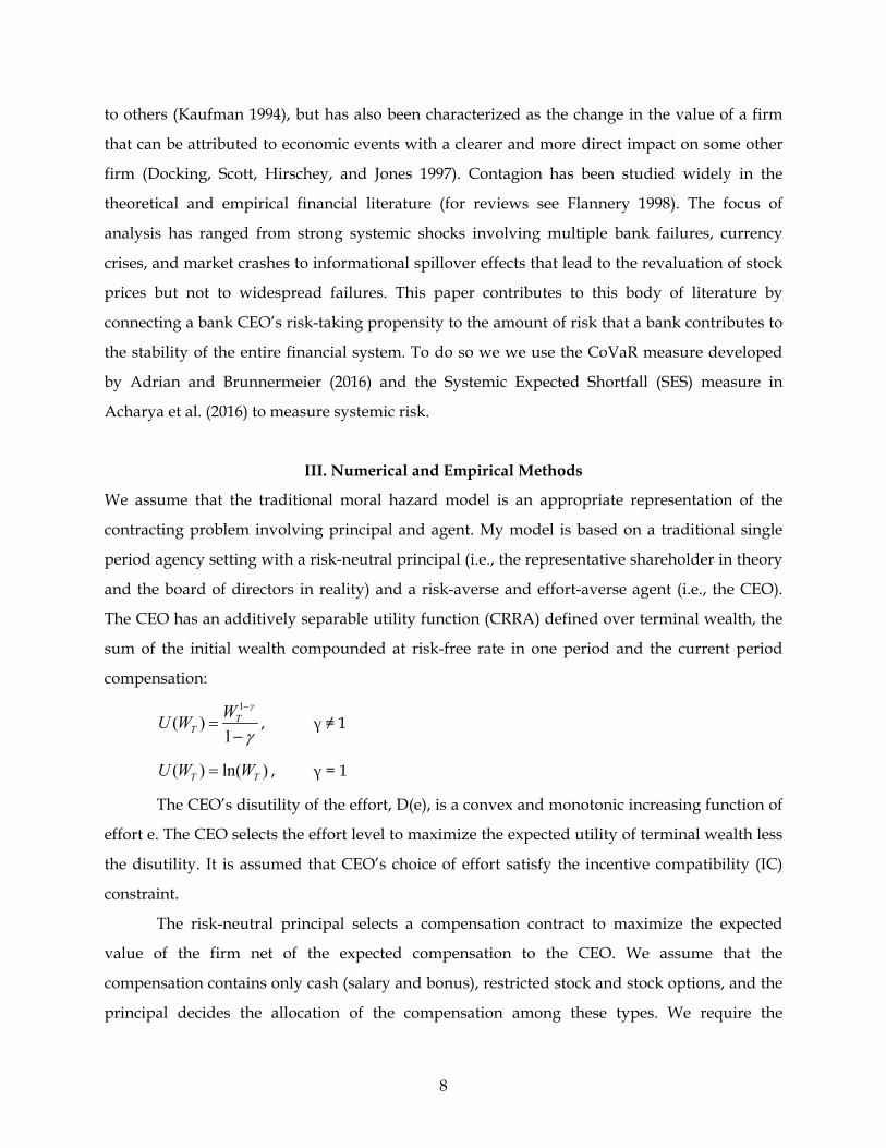
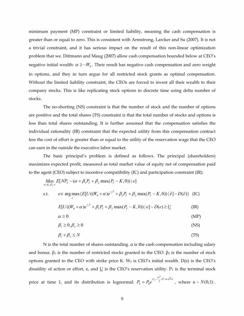
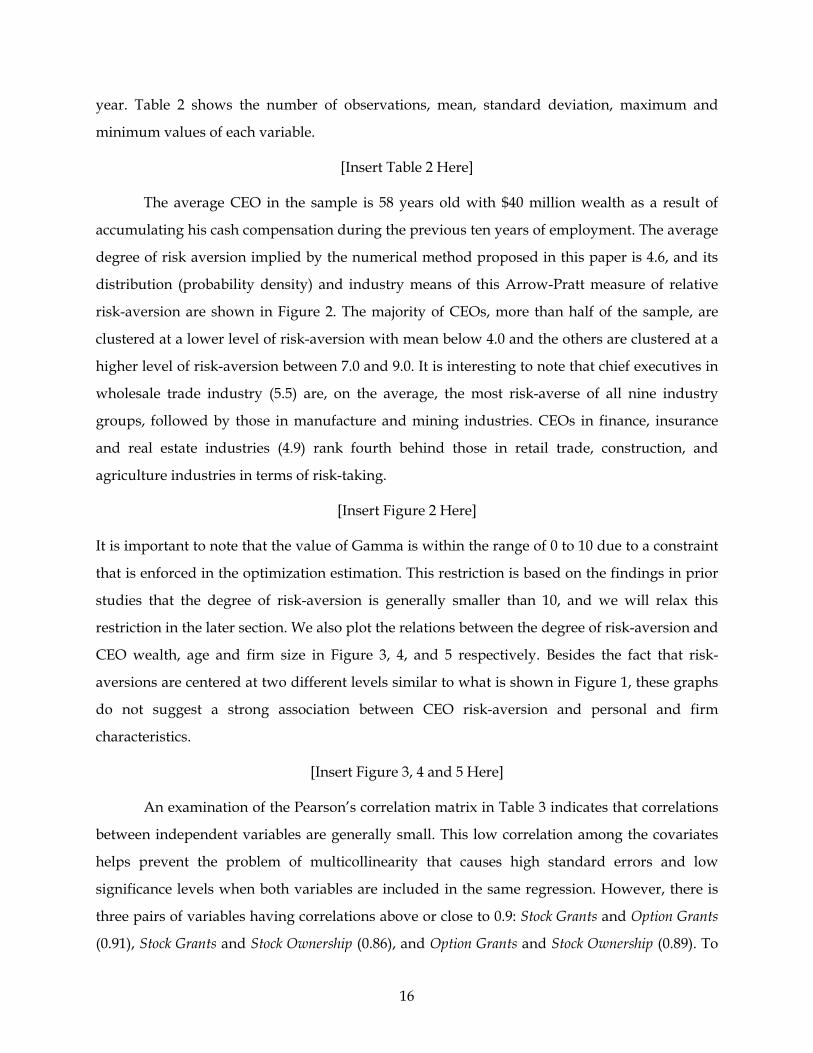
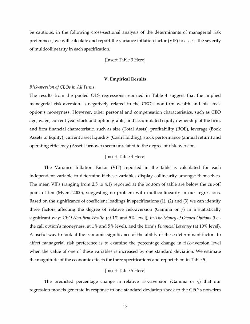
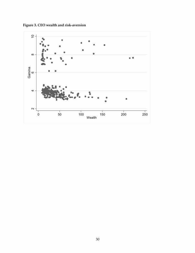
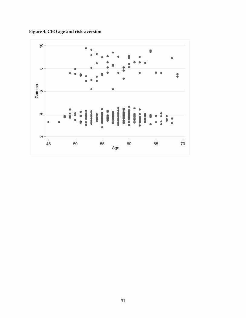
restriction in the later section. We also plot the relations between the degree of risk-aversion and

CEO wealth, age and firm size in Figure 3, 4, and 5 respectively. Besides the fact that risk-

aversions are centered at two different levels similar to what is shown in Figure 1, these graphs

do not suggest a strong association between CEO risk-aversion and personal and firm

characteristics.

[Insert Figure 3, 4 and 5 Here]

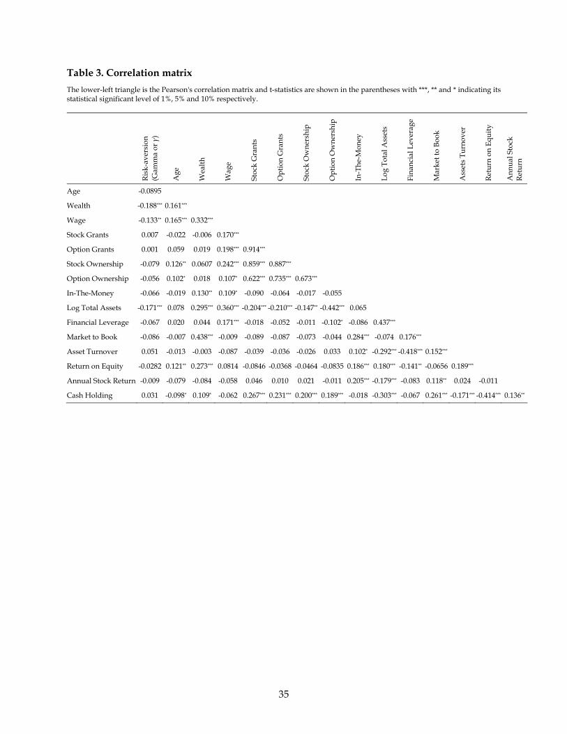
An examination of the Pearson’s correlation matrix in Table 3 indicates that correlations

between independent variables are generally small. This low correlation among the covariates

helps prevent the problem of multicollinearity that causes high standard errors and low

significance levels when both variables are included in the same regression. However, there is

three pairs of variables having correlations above or close to 0.9: Stock Grants and Option Grants

(0.91), Stock Grants and Stock Ownership (0.86), and Option Grants and Stock Ownership (0.89). To

17

be cautious, in the following cross-sectional analysis of the determinants of managerial risk

preferences, we will calculate and report the variance inflation factor (VIF) to assess the severity

of multicollinearity in each specification.

[Insert Table 3 Here]

V. Empirical Results

Risk-aversion of CEOs in All Firms

The results from the pooled OLS regressions reported in Table 4 suggest that the implied

managerial risk-aversion is negatively related to the CEO’s non-firm wealth and his stock

option’s moneyness. However, other personal and compensation characteristics, such as CEO

age, wage, current year stock and option grants, and accumulated equity ownership of the firm,

and firm financial characteristic, such as size (Total Assts), profitability (ROE), leverage (Book

Assets to Equity), current asset liquidity (Cash Holding), stock performance (annual return) and

operating efficiency (Asset Turnover) seem unrelated to the degree of risk-aversion.

[Insert Table 4 Here]

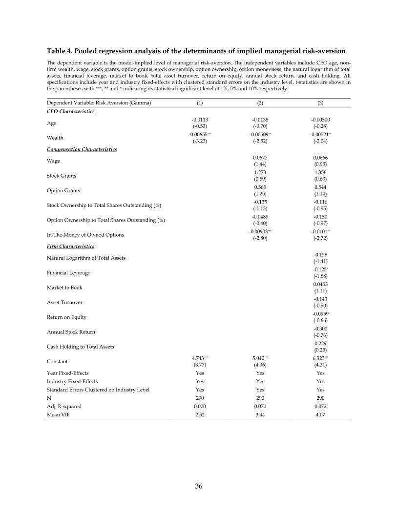
The Variance Inflation Factor (VIF) reported in the table is calculated for each

independent variable to determine if these variables display collinearity amongst themselves.

The mean VIFs (ranging from 2.5 to 4.1) reported at the bottom of table are below the cut-off

point of ten (Myers 2000), suggesting no problem with multicollinearity in our regressions.

Based on the significance of coefficient loadings in specifications (1), (2) and (3) we can identify

three factors affecting the degree of relative risk-aversion (Gamma or γ) in a statistically

significant way: CEO Non-firm Wealth (at 1% and 5% level), In-The-Money of Owned Options (i.e.,

the call option’s moneyness, at 1% and 5% level), and the firm’s Financial Leverage (at 10% level).

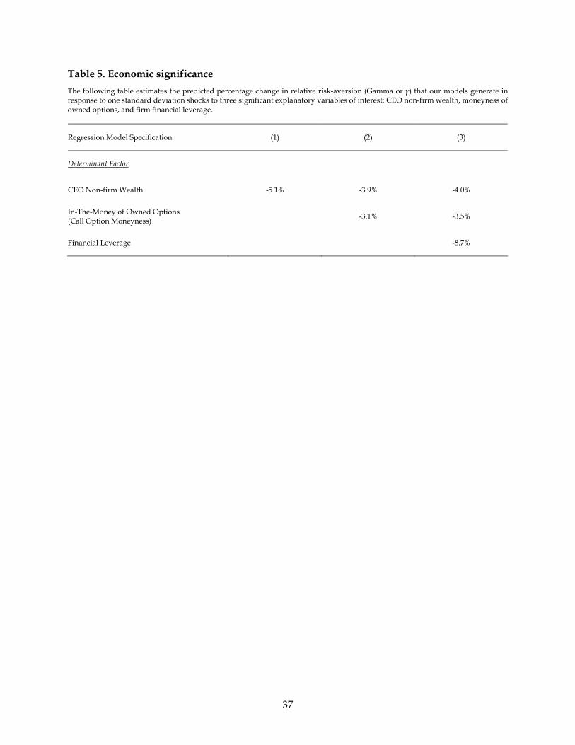
A useful way to look at the economic significance of the ability of these determinant factors to

affect managerial risk preference is to examine the percentage change in risk-aversion level

when the value of one of these variables is increased by one standard deviation. We estimate

the magnitude of the economic effects for three specifications and report them in Table 5.

[Insert Table 5 Here]

The predicted percentage change in relative risk-aversion (Gamma or γ) that our

regression models generate in response to one standard deviation shock to the CEO’s non-firm

18

wealth is -5.1%, -3.9%, and -4.0% for regression specifications (1), (2), and (3) respectively.

Similarly, the changes in managerial risk-aversion are -3.5% and -8.7% in response to one

standard deviation change in the CEO’s option portfolio moneyness and the firm’s financial

leverage. These results are robust to perturbation of study variates and methods in estimating

the degree of risk aversion by calculating CEO wealth using 5-year income data and by adding

[-10%,+10%] random disturbance to the values of individual wealth, wage, stock grants, option

grants, stock ownership, option ownership, and in-the-money of options. We create a new

sample by requiring CEO compensation contract information exist in the Executive

Compensation database for at least five consecutive years rather than ten consecutive years as

in the previous results.

[Insert Table 6 Here]

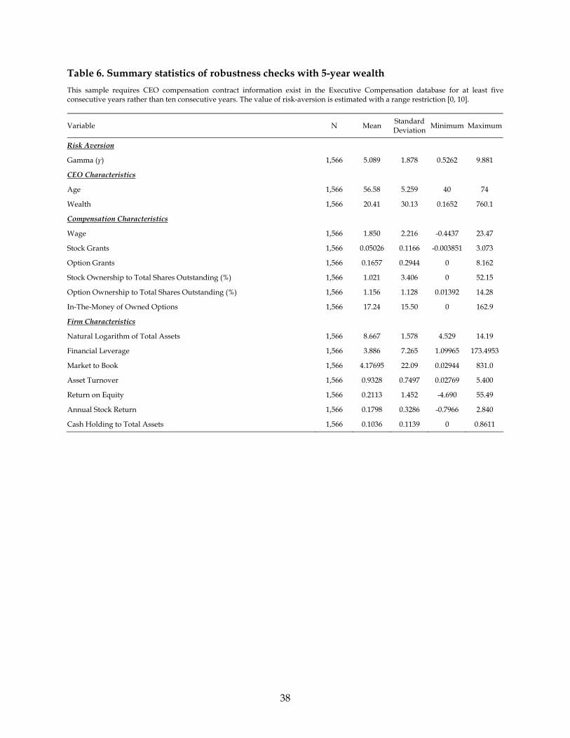
The summary statistics in Table 6 show that not only the sample size is larger but also

the estimated level of risk aversion (5.1) is slightly higher than the one obtained in the previous

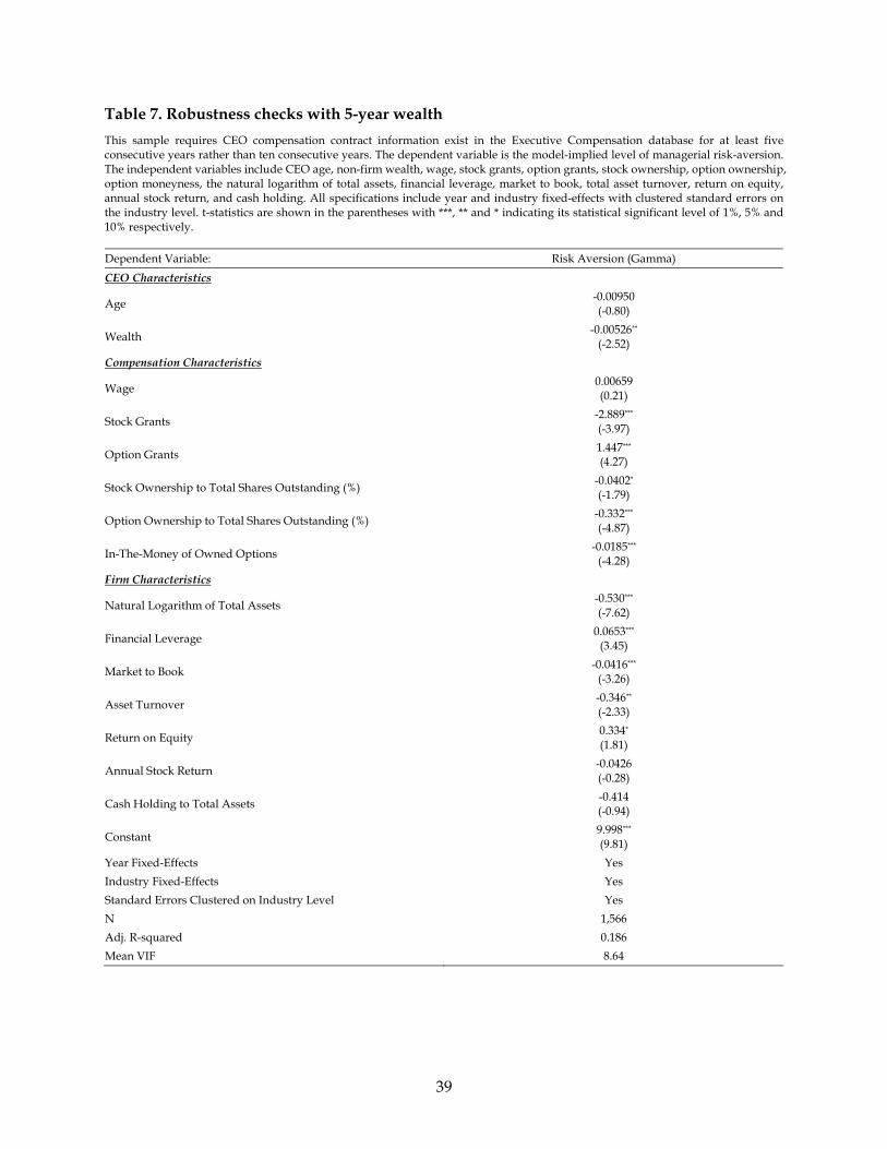
results (4.6). We repeat our pooled regression analysis using this new data set and the

coefficient estimates are reported in Table 7. In addition to the negative effects of CEO wealth

and option in-the-money, a CEO’s risk-aversion is positively related to her stock grants and the

firm’s financial leverage and negatively related to her option ownership and the firm’s size

(total assets), market-to-book, and asset turnover.

[Insert Table 7 Here]

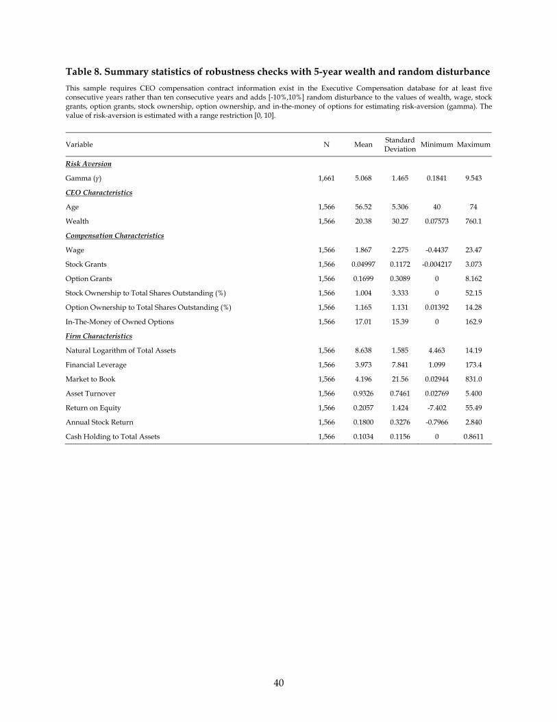
In the next robustness check, we add [-10%,+10%] random disturbance to the values of

individual wealth, wage, stock grants, option grants, stock ownership, option ownership, and

in-the-money of options and re-estimate the degree of CEO risk-aversion. The summary

statistics in Table 8 and regression results in Table 9 are similar to the ones obtained in the

previous robustness test.

[Insert Table 8 and Table 9 Here]

Risk-aversion of Bank CEOs and Systemic Risk

To understand the relationship between the degree of risk-taking of a bank CEO and the

amount of contagion risk that the bank contributes to the entire financial system, we regress the

19

level of systemic risk on the measure of CEO’s risk-aversion along with other control variables.

Table 10 shows the summary statistics of this rather small sample that only includes CEOs of

bank holding companies.

[Insert Table 10 Here]

Still, the sample size (N=561) is larger than that of the first sample (N=290) in Table 2. The

reason is due to two relaxed constraints in sample construction and numerical estimation. The

first one is the elimination of 10-year tenure requirement in the same firm. Instead, we use the

future value of 10-year annuity payment formula to calculate the initial non-firm wealth of the

CEO where r is the average annual interest rate, CF is approximated by the total compensation

in dollars in including salary, bonus and, restricted stock and stock options :

10(1 ) 1r

Ordinary Annuity rFV CF

The second relaxed constraint is the requirement that the value of Gamma is within the range of

0 to 10. Unfortunately, when this constraint is strictly enforced as shown in the first half of the

tests in this paper, many firm-CEO pairs may not have feasible solutions. Because we suspect

that this restriction is too strong to be of much use, we will relax it to be within the range of 0 to

20 in risk-aversion estimation.

The average CEO age (58 year-old) and initial non-firm wealth ($40 million) in this bank

CEO sample are similar to those in the previous two samples. The average implied-risk

aversion is 15 and this is larger than that of previous findings is due to the relaxed restriction on

the range of Gamma (0 to 20). The first two cross-sectional muntivariate tests are based on

pooled OLS regression with year fixed-effects. The specifications in Table 11 have ∆CoVaR as

the measure of a bank’s systemic risk on the LHS and the Gamma, the degree of risk-aversion of

bank CEOs, on the RHS. The finding is somewhat surprising: after controlling for CEO and

bank characteristics (e.g., age, wealth, wage, stock grants, option grants, stock ownership,

option ownership, option moneyness, the natural logarithm of total assets, financial leverage,

market to book, liquidity, return on asset, annual stock return, loan portfolios, and loan

commitment), the risk-taking incentives embedded in the compensation contract of a bank CEO

is not related to the amount of contagion risk that this bank contributes to the banking system,

Although the signs of Risk-Aversion are negative, they not statistically significant in all

regression specifications.

20

[Insert Table 11 Here]

The regressions in Table 12 use SES as the measure of a bank’s systemic risk, proxying

for the vulnerability of a bank to the financial stability of the entire banking system, on the LHS

and the Gamma, the degree of risk-aversion of bank CEOs, on the RHS. Again, there is no

statistical association between these two variables, suggesting that a risk-taking CEO of a bank

holding company is not necessarily make the bank vulnerable to contagion risk.

[Insert Table 12 Here]

While the evidence presented thus far is convincing, it is still possible that the omitted variable

problem (i.e., unobserved CEO and firm characteristics) may have biased the coefficient

estimates. In the following two tests we include firm fixed-effects, in addition to year fixed-

effects in the previous regression specifications, to exploit the variation over time in our

measures of bank CEO risk-aversion as reflected by the risk-taking incentives embedded in the

executive compensation contract. The basic specifications in Table 13 and Table 14 are same as

the ones in Table 11 and Table 12 respectively, except including the bank fixed-effects. The

insignificant coefficient estimates of Risk-Aversion remain in both tables, suggesting that even

the risk-taking incentives increase in the compensation contract, they do not necessarily increase

the contagion risk of the bank.

[Insert Table 13 and Table 14 Here]

Finally, it is noted in Dittmann and Maug (2007) that the calibration of a principal-agent

model using observed data is sensitive to the CEO’s non-firm wealth, which is often not

observable, and each of the two estimation methods of CEO wealth presented in this research

has its limitations. In the first method, the requirement of 10-year or 5-year continuous

compensation data of a CEO in the Execcomp dataset reduces the sample size. It is often the

case that some of them left the sample and then reappeared in a later year. In the second

method, whereas the use of 10-year annuity payment formula based on one-year income data

(cash flow in the initial year) helps increase the sample size, it has to assume that future incomes

do not fluctuate over time. Therefore, as a robustness check, we combine both estimation

methods to create a simple two-stage method to predict CEO wealth. In the first stage, we

conduct a pooled OLS regression on a sample of CEOs with 10-year accumulated wealth (from

21

the first method) to estimate the relationship between the 10-year accumulated wealth and the

cash flow in the initial year (used in the second method):

, , , ,i t i t i t t i tWealth Cashflow Age

In the second stage, we use the coefficient estimates (α, β, γ, and λ) and the income cash flow

and CEO age in each year in the larger sample (for the second method) to predict a CEO’s

wealth:

, , , ,ˆ ˆˆ ˆ ˆi t i t i t t i tW CF AGE

After obtaining the fitted wealth, we repeat the regression models in Tables 13 and 14. Overall,

the insignificant coefficient estimates of risk-aversion shown in Tables 15 and 16 confirm our

previous findings that risk-taking preference of bank CEOs is not related to the bank’s systemic

risk measured in both CoVaR and SES.

[Insert Table 15 and Table 16 Here]

VI. Discussion and Conclusion

Fitting a principal-agent model using observed executive compensation data produces a

number of insights that have not been presented in the empirical corporate finance literature.

We find a very low degree of risk-aversion among CEOs with the average Arrow-Pratt measure

of relative risk-aversion (CRRA) being 4.6 for 290 managers who have served as CEOs for more

than ten years. This result is, to some extent, consistent with the theoretical finding in the

previous studies. For example, Hemmer, Kim and Verrecchia (2000) use a principal–agent

model to show that in the case of log utility, if relative risk aversion is less than one, the optimal

contract is convex in stock value. The assumptions behind our numerical estimation method are

“optimal effort” and “optimal pay”. The first one means that when a manager accepts the offer

of employment to become or continue to serve as the CEO of the firm, the compensation

contract reflects the optimal level of efforts that the CEO will and must exert in order to

maximize the firm value. The optimal pay assumption suggests that the observed compensation

contract offered by the firm has already attained the level at the lowest cost to the firm.

To better understand the cross-sectional variation of managerial risk preferences, we

study the determinants of the model-implied risk-aversion by conducting pooled OLS

22

regression and identified two factors that are negatively related to CEO risk-aversion: CEO

wealth and their options portfolio’s moneyness. Other personal and compensation

characteristics, such as CEO age, wage, current year stock and option grants, and accumulated

equity ownership of the firm, and firm financial characteristic, such as size, profitability,

leverage, liquidity and operating efficiency, seem unrelated to CEO risk-aversion.

Perhaps the most striking result from this research is a non-result: the lack of

relationship between bank CEOs’ risk-taking incentives and systemic risk in a very important

financial sector: banking. Executive compensation policy has been controversial within the

corporate finance literature and mainstream media and often blamed for encouraging excessive

risk-taking in financial services that stoked the global economic crisis in 2008-10. Yet, the

evidence presented here does not seem to support the claim that risk-taking incentives

embedded in the executive compensation contracts in U.S. banks are related to contagion risk in

the banking sector.

In sum, we find somewhat mixed evidence in favor of the presence of excessive risk

taking among CEOs in many industries including banking. When interpreting the evidence

presented in this paper, however, it is important to bear in mind that our results rely on the

critical assumption of an efficient managerial labor market. The competitive equilibrium in the

CEO labor market is reflected in the observed CEO compensation contract which indicates the

optimal level of the CEO’s effort and the lowest cost to the firm. If these conditions hold, the

actual managerial pay is an unbiased estimate of the CEO’s expected marginal contribution to

the firm’s outcome. As Kaplan (2008) points out, although far from perfect, CEO pay practices

are mainly driven by market competition. On one hand, if a CEO thinks the pay is too low, he

will not accept the job offer and take another post offering higher pay. On the other hand, a

high paying job creates competition among CEOs, and only the best performer gets the job,

hence exerting maximum effort. Furthermore, it can be argued that in reality the principal-agent

model is not an appropriate model to describe the relationship between the shareholders and

the CEO. Nevertheless, we believe one important contribution of this paper is to provide a

relatively clean framework for evaluating managerial risk preferences embedded in the

observed executive compensation contracts.

23

REFERENCE

Acharya, Viral, Lasse Pedersen, Thomas Philippon, and Mathew Richardson, 2016, Measuring Systemic Risk, Review of Financial Studies, 30, 2–47. Ackerberg, Daniel and Maristella Botticini, 2002, Endogenous Matching and the Empirical Determinants of Contract Form, Journal of Political Economy, 110, 564–591. Adrian, Tobias and Markus Brunnermeier, 2016, CoVaR, American Economic Review, 106, 1705–1741. Ait-Sahalia, Yacine and Andrew Lo, 1998, Nonparametric estimation of state-price densities implicit in financial asset prices, Journal of Finance, 53, 499–547. Ait-Sahalia, Yacine and Andrew Lo, 2000, Non-parametric Risk Management and Implied Risk Aversion, Journal of Econometrics, 94, 9–51. Allen, Douglas and Dean Lueck, 1995, Risk Preferences and the Economics of Contracts, American Economic Review, Papers and Proceedings, 85, 447–451. Armstrong, Christopher, David Larcker and Che-Lin Su, 2007, Working Paper, Stanford University and Northwestern University. Arrow, Kenneth, 1971, Essays in the Theory of Risk Bearing. North Holland, Amsterdam. Aseff, Jorge and Manuel Santos, 2005, Stock Options and Managerial Optimal Contracts, Economic Theory, 26, 813–837. Bebchuk, Lucian, 2009, Regulate financial pay to reduce risk-taking, Opinion, Financial Times, August 3rd. Becker, Bo, 2006, Wealth and Executive Compensation, Journal of Finance, 61, 1, 379–397. Bennett, Rosalind, Levent Guntay and Haluk Unal, 2015, Inside Debt, Bank Default Risk and Performance during the Crisis, Journal of Financial Intermediation, 24, 487–513. Bettis, J. Carr, John Bizjak, and Michael Lemmon, 2005, Exercise behavior, valuation, and the incentive effects of employee stock options, Journal of Financial Economics, 76, 445–470. Bliss, R.R., and N. Panigirtzoglou, 2002, Testing the stability of implied probability density functions, Journal of Banking and Finance, 26, 381–422. Bliss, R.R., and N. Panigirtzoglou, 2004, Option-implied risk aversion estimates, Journal of Finance, 59, 407–446. Borghans, Lex, James Heckman, Bart Golsteyn, and Huub Meijers, 2009, Gender differences in risk aversion and ambiguity aversion, Journal of European Economic Association, 7, 649–658.

24

Brunnermeier, Markus, G. Nathan Dong, and Darius Palia, 2012, Non-interest Income and Systemic Risk, AFA 2012 Chicago Meetings Paper. Cain, Matthew and Stephen McKeon, 2016, CEO Personal Risk-Taking and Corporate Policies, Journal of Financial and Quantitative Analysis, 51, 139–164. Calluzzo, Paul and Gang Nathan Dong, 2015, Has the financial system become safer after the crisis? The changing nature of financial institution risk, Journal of Banking and Finance, 53, 233–248. Campbell, John, Andrew Lo and Craig McKinlay, 1997, The Econometrics of Financial Markets, Princeton University Press. Carpenter, Jennifer, 2000, Does Option Compensation Increase Managerial Risk Appetite, Journal of Finance, 55, 2311–2331. Dittmann, Ingolf and Ernst Maug, 2007, Lower Salaries and No Options? On the Optimal Structure of Executive Pay, Journal of Finance, 62, 303–343. Docking, Diane Scott, Mark Hirschey, and Elaine Jones, 1997, Information and Contagion Effects of Bank Loan-Loss Reserve Announcements, Journal of Financial Economics, 43, 219–239. Dohmen, Thomas, Armin Falk, David Huffmann, and Uwe Sunde, 2010, Are Risk Aversion and Impatience Related to Cognitive Ability?, American Economic Review, 100, 1238–1260. Dong, Gang Nathan, 2014, Excessive financial services CEO pay and financial crisis: Evidence from calibration estimation, Journal of Empirical Finance, 27, 75–96. Epstein, Larry and Stanley Zin, 1991, Substitution, Risk Aversion and the Temporal Behaviour of Consumption and Asset Returns: An Empirical Analysis, Journal of Political Economy, 99, 263–268. Fahlenbrach, Rudiger and Rene Stulz, 2011, Bank CEO Incentives and the Credit Crisis, Journal of Financial Economics, 99, 11–26. Ferson, Wayne and George Constantinides, 1991, Habitat Persistence and Durability in Aggregate Consumption: Empirical Tests, Journal of Financial Econometrics, 29, 199–240. Flannery, Mark J., 1998, Using Market Information in Prudential Bank Supervision: A Review of the U.S. Empirical Evidence, Journal of Money, Credit, and Banking, 30, 273–305. Friend, Irwin and Marshall Blume, 1975, The Demand for Risky Assets, American Economic Review, 65, 900–922. Gauthier, Celine, Alfred Lehar, and Moez Souissi, 2012, Macroprudential Capital Requirements and Systemic Risk, Journal of Financial Intermediation, 21, 594–618.

25

Guo, Hui and Robert Whitelaw, 2006, Uncovering the Risk-Return Relation in the Stock Market, Journal of Finance, 61, 1433–1463. Grahama, John, Campbell Harvey, and Manju Puri, 2013, Managerial attitudes and corporate actions, Journal of Financial Economics, 109, 103–121. Hall, Brian and Kevin Murphy, 2000, Optimal Exercise Prices for Executive Stock Options, American Economic Review, 90, 209–214. Hall, Brian and Kevin Murphy, 2002, Stock Options for Undiversified Executives, Journal of Accounting and Economics, 33, 3–42. Hansen, Lars and Kenneth Singleton, 1982, Generalized Instrumental Variables Estimation of Nonlinear Rational Expectations Models, Econometrica, 50, 1269–1286. Hansen, Lars and Kenneth Singleton, 1984, Errata: Generalized Instrumental Variables Estimation of Nonlinear Rational Expectations Models, Econometrica, 52, 267–268. Hemmer, T., O. Kim, and R.E. Verrecchia, 2000, Introducing convexity into optimal compensation contracts, Journal of Accounting and Economics, 28, 307–327. Holmstrom, Bengt, 1979, Moral Hazard and Observability, Bell Journal of Economics, 10, 74–91. Ingersoll, Jonathan, 1998, Approximating American options and other financial contracts using barrier derivatives, Journal of Computational Finance, 2, 85–112. International Accounting Standards Board, 2004, Share-Based Payment. International Financial Reporting Standards 2. Jensen, Michael and William Meckling, 1976, Theory of the Firm: Managerial Behavior, Agency Costs, and Ownership Structure, Journal of Financial Economics, 3, 305–360. Jorion, Philippe and Alberto Giovannini, 1993, Time Series Test of a Non-Expected Utility Model of Asset Pricing, European Economic Review, 37, 1083–1100. Kadan and Swinkels, Forthcoming, Stock or Options? Moral Hazard, Firm Viability, and the Design of Compensation Contracts, 2008, Review of Financial Studies, 21, 451–482. Kang, B.J., T.S. Kim, 2006, Option implied risk preferences: an extension to wider classes of utility functions, Journal of Financial Markets, 9, 180–198. Kaplan, Steven, 2008, Are U.S. CEOs Overpaid?, Academy of Management Perspectives, 22, 5–20. Kaufman, George, 1994, Bank Contagion: A Review of the Theory and Evidence. Journal of Financial Services Research, 8, 123–150.

26

Lambert, Richard, David Larcker and Robert Verrecchia, 1991, Portfolio Considerations in Valuing Executive Compensation, Journal of Accounting Research, 29, 129-149. Lewellen, K., 2006, Financing decisions when managers are risk averse, Journal of Financial Economics 82, 551–589. MacCrimmon, Kenneth and Donald Wehrung, 1990, Characteristics of Risk Taking Executives, Management Science, 36, 422–435. Mann, H. B., and D.R. Whitney, 1947, On a Test of Whether One of Two Random Variables is Stochastically Larger Than the Other, Annals of Mathematical Statistics, 18, 50–60. Mehran, Hamid, 1995, Executive Compensation Structure, Ownership, and Firm Performance, Journal of Financial Economics, 38, 163–184. Meulbroek, Lisa, 2001, The Efficiency of Equity-linked Compensation: Understanding the Full Cost of Awarding Executive Stock Options, Financial Management, 30, 5–30. Murphy, Kevin, 1999, Executive compensation, Handbook of Labor Economics 3, 2485–2563, North Holland, Amsterdam. Murphy, Kevin, 2013, Regulating Banking Bonuses in the European Union: a Case Study in Unintended Consequences, European Financial Management, 19, 631–657. Myers, Raymons, 2000, Classical and Modern Regression with Applications, Duxbury Press, Boston, MA. Normandin, Michel and Pascal St-Amour, 1998, Substitution, Risk Aversion, Taste Shocks and Equity Premia, Journal of Applied Econometrics, 13, 265–281. Rivlin, Alice, 2009, Reducing Systemic Risk in the Financial Sector, Testimony before the Housing Committee on Financial Services, July 21st. Ross, Stephen, 2004, Compensation, Incentives, and the Duality of Risk Aversion and Riskiness, Journal of Finance, 59, 207-225. Santomero, Anthony and Jeffrey Trester, 1998, Financial innovation and bank risk taking, Journal of Economic Behavior & Organization, 35, 25–37. Securities and Exchange Commission, 2005, Staff Accounting Bulletin No. 107. Securities and Exchange Commission, 2015, Pay Ratio Disclosure, 17 CFR Parts 229 and 249. Shaw, Kathryn, 1996, An Empirical Analysis of Risk Aversion and Income Growth, Journal of Labor Economics, 14, 626–653.

27

Skaperdas, Stergios and Gan Li, 1995, Risk Aversion in Contests, Economic Journal, 105, 951–962. Wilcoxon, F., 1945, Individual Comparisons by Ranking Methods, Biometrics Bulletin, 1, 80–83.

28

Figure 1. CEO risk-aversion over time

Mean value 0

12

34

56

Gam

ma

1997

1998

1999

2000

2001

2002

2003

2004

2005

2006

2007

2008

2009

2010

2011

2012

2013

Upper adjacent value, 75th percentile, median, 25th percentile, and lower adjacent value

23

45

67

89

10G

amm

a

1997

1998

1999

2000

2001

2002

2003

2004

2005

2006

2007

2008

2009

2010

2011

2012

2013

excludes outside values

29

Figure 2. Distribution of CEO risk-aversion

Density of risk-aversion measured in Gamma 0

.2.4

.6.8

De

nsity

2 4 6 8 10Gamma

Industry mean of CEO risk-aversion

4.2

5.1

4.5

5.25

5.5

4.64.9

5

01

23

45

6G

amm

a

Agricu

lture

, For

estry

Mini

ng

Constr

uctio

n

Man

ufac

turin

g

Trans

porta

tion,

Com

mun

icatio

ns, U

tilitie

s

Who

lesa

le T

rade

Retail

Tra

de

Finan

ce, I

nsur

ance

, Rea

l Esta

te

Servic

es

30

Figure 3. CEO wealth and risk-aversion

24

68

10G

amm

a

0 50 100 150 200 250Wealth

31

Figure 4. CEO age and risk-aversion

24

68

10G

amm

a

45 50 55 60 65 70Age

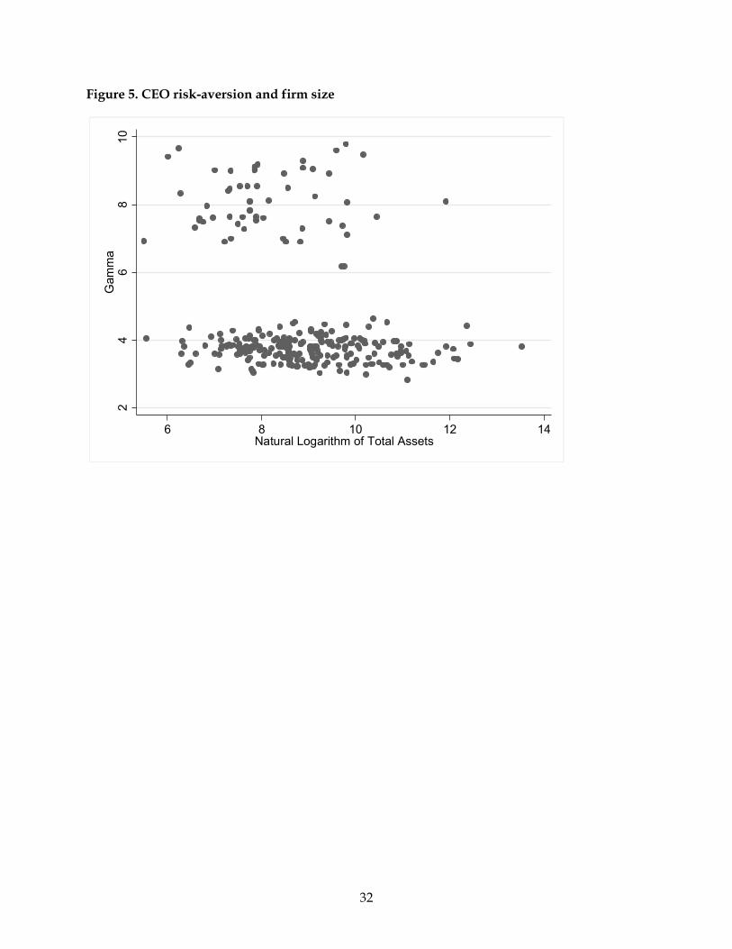
32

Figure 5. CEO risk-aversion and firm size

24

68

10G

amm

a

6 8 10 12 14Natural Logarithm of Total Assets

33

Table 1. Variable definitions Variable Name Definition

Risk Aversion

Gamma (γ) Risk aversion measure

CEO Characteristics

Age Age in years

Wealth ($ thousand) Total wealth ÷ 1,000

Compensation Characteristics log(Total assets)

Wage ($ thousand) Current year cash-based salary ÷ 1,000

Stock Grants (Current year granted stocks ÷ Total shares outstanding) × 100

Option Grants (Current year granted options ÷ Total shares outstanding) × 100

Stock Ownership to Total Shares Outstanding (%) (All granted stocks ÷ Total shares outstanding) × 100

Option Ownership to Total Shares Outstanding (%) (All granted options ÷ Total shares outstanding) × 100

In-The-Money of Owned Options Stock Price – Average strike of all granted options

Firm Characteristics

Natural Logarithm of Total Assets log(Total assets)

Financial Leverage Total assets ÷ Book equity

Market to Book Stock market value ÷ Book equity

Asset Turnover Revenue ÷ Total assets

Return on Equity Net income ÷ Book equity

Annual Stock Return Accumulated stock return during the year

Cash Holding to Total Assets (Cash + Cash equivalents) ÷ Total assets

34

Table 2. Summary statistics

The value of risk-aversion is estimated with a range restriction [0, 10].

Variable N Mean Standard Deviation

Minimum Maximum

Risk Aversion

Gamma (γ) 290 4.613 1.836 2.820 9.795

CEO Characteristics

Age 290 57.74 4.754 45 74

Wealth 290 40.47 35.74 4.921 222.0

Compensation Characteristics

Wage 290 1.663 1.460 0.3079 8.803

Stock Grants 290 0.0434 0.1288 0.0004 2.096

Option Grants 290 0.1682 0.4921 0.0063 8.162

Stock Ownership to Total Shares Outstanding (%) 290 0.8832 3.345 0.0037 52.15

Option Ownership to Total Shares Outstanding (%) 290 1.224 1.313 0.0156 14.28

In-The-Money of Owned Options 290 16.61 15.83 0 120.4

Firm Characteristics

Natural Logarithm of Total Assets 290 8.801 1.358 5.505 13.53

Financial Leverage 290 3.587 3.203 1.159 24.01

Market to Book 290 3.740 3.018 0.4543 24.08

Asset Turnover 290 0.9051 0.6385 0.0386 3.681

Return on Equity 290 0.1653 0.3331 -4.691 1.084

Annual Stock Return 290 0.1733 0.3137 -0.6784 2.559

Cash Holding to Total Assets 290 0.1108 0.1147 0.0005 0.8051

35

Table 3. Correlation matrix

The lower-left triangle is the Pearson's correlation matrix and t-statistics are shown in the parentheses with ***, ** and * indicating its statistical significant level of 1%, 5% and 10% respectively.

Ris

k-av

ersi

on

(Gam

ma

or γ

)

Age

Wea

lth

Wag

e

Stoc

k G

rant

s

Op

tion

Gra

nts

Stoc

k O

wne

rshi

p

Op

tion

Ow

ners

hip

In-T

he-M

oney

Log

Tot

al A

sset

s

Fina

ncia

l Lev

erag

e

Mar

ket t

o B

ook

Ass

ets

Tur

nove

r

Ret

urn

on E

quit

y

Ann

ual S

tock

R

etu

rn

Age -0.0895

Wealth -0.188*** 0.161***

Wage -0.133** 0.165*** 0.332***

Stock Grants 0.007 -0.022 -0.006 0.170***

Option Grants 0.001 0.059 0.019 0.198*** 0.914***

Stock Ownership -0.079 0.126** 0.0607 0.242*** 0.859*** 0.887***

Option Ownership -0.056 0.102* 0.018 0.107* 0.622*** 0.735*** 0.673***

In-The-Money -0.066 -0.019 0.130** 0.109* -0.090 -0.064 -0.017 -0.055

Log Total Assets -0.171*** 0.078 0.295*** 0.360*** -0.204*** -0.210*** -0.147** -0.442*** 0.065

Financial Leverage -0.067 0.020 0.044 0.171*** -0.018 -0.052 -0.011 -0.102* -0.086 0.437***

Market to Book -0.086 -0.007 0.438*** -0.009 -0.089 -0.087 -0.073 -0.044 0.284*** -0.074 0.176***

Asset Turnover 0.051 -0.013 -0.003 -0.087 -0.039 -0.036 -0.026 0.033 0.102* -0.292*** -0.418*** 0.152***

Return on Equity -0.0282 0.121** 0.273*** 0.0814 -0.0846 -0.0368 -0.0464 -0.0835 0.186*** 0.180*** -0.141** -0.0656 0.189***

Annual Stock Return -0.009 -0.079 -0.084 -0.058 0.046 0.010 0.021 -0.011 0.205*** -0.179*** -0.083 0.118** 0.024 -0.011

Cash Holding 0.031 -0.098* 0.109* -0.062 0.267*** 0.231*** 0.200*** 0.189*** -0.018 -0.303*** -0.067 0.261*** -0.171*** -0.414*** 0.136**

36

Table 4. Pooled regression analysis of the determinants of implied managerial risk-aversion

The dependent variable is the model-implied level of managerial risk-aversion. The independent variables include CEO age, non-firm wealth, wage, stock grants, option grants, stock ownership, option ownership, option moneyness, the natural logarithm of total assets, financial leverage, market to book, total asset turnover, return on equity, annual stock return, and cash holding. All specifications include year and industry fixed-effects with clustered standard errors on the industry level. t-statistics are shown in the parentheses with ***, ** and * indicating its statistical significant level of 1%, 5% and 10% respectively. Dependent Variable: Risk Aversion (Gamma) (1) (2) (3)

CEO Characteristics

Age -0.0113 (-0.53)

-0.0138 (-0.70)

-0.00500 (-0.28)

Wealth -0.00655***

(-3.23) -0.00509**

(-2.52) -0.00521**

(-2.04)

Compensation Characteristics

Wage

0.0677 (1.44)

0.0666 (0.95)

Stock Grants

1.273 (0.59)

1.356 (0.63)

Option Grants

0.565 (1.25)

0.544 (1.14)

Stock Ownership to Total Shares Outstanding (%)

-0.135 (-1.13)

-0.116 (-0.95)

Option Ownership to Total Shares Outstanding (%)

-0.0489 (-0.40)

-0.150 (-0.97)

In-The-Money of Owned Options

-0.00903*** (-2.80)

-0.0101** (-2.72)

Firm Characteristics

Natural Logarithm of Total Assets

-0.158 (-1.41)

Financial Leverage

-0.125* (-1.88)

Market to Book

0.0453 (1.11)

Asset Turnover

-0.143 (-0.50)

Return on Equity

-0.0959 (-0.66)

Annual Stock Return

-0.300 (-0.76)

Cash Holding to Total Assets

0.229 (0.25)

Constant 4.743*** (3.77)

5.040*** (4.36)

6.323*** (4.31)

Year Fixed-Effects Yes Yes Yes

Industry Fixed-Effects Yes Yes Yes

Standard Errors Clustered on Industry Level Yes Yes Yes

N 290 290 290

Adj. R-squared 0.070 0.070 0.072

Mean VIF 2.52 3.44 4.07

37

Table 5. Economic significance

The following table estimates the predicted percentage change in relative risk-aversion (Gamma or γ) that our models generate in response to one standard deviation shocks to three significant explanatory variables of interest: CEO non-firm wealth, moneyness of owned options, and firm financial leverage.

Regression Model Specification (1) (2) (3)

Determinant Factor

CEO Non-firm Wealth -5.1% -3.9% -4.0%

In-The-Money of Owned Options (Call Option Moneyness)

-3.1% -3.5%

Financial Leverage -8.7%

38

Table 6. Summary statistics of robustness checks with 5-year wealth

This sample requires CEO compensation contract information exist in the Executive Compensation database for at least five consecutive years rather than ten consecutive years. The value of risk-aversion is estimated with a range restriction [0, 10].

Variable N Mean Standard Deviation

Minimum Maximum

Risk Aversion

Gamma (γ) 1,566 5.089 1.878 0.5262 9.881

CEO Characteristics

Age 1,566 56.58 5.259 40 74

Wealth 1,566 20.41 30.13 0.1652 760.1

Compensation Characteristics

Wage 1,566 1.850 2.216 -0.4437 23.47

Stock Grants 1,566 0.05026 0.1166 -0.003851 3.073

Option Grants 1,566 0.1657 0.2944 0 8.162

Stock Ownership to Total Shares Outstanding (%) 1,566 1.021 3.406 0 52.15

Option Ownership to Total Shares Outstanding (%) 1,566 1.156 1.128 0.01392 14.28

In-The-Money of Owned Options 1,566 17.24 15.50 0 162.9

Firm Characteristics

Natural Logarithm of Total Assets 1,566 8.667 1.578 4.529 14.19

Financial Leverage 1,566 3.886 7.265 1.09965 173.4953

Market to Book 1,566 4.17695 22.09 0.02944 831.0

Asset Turnover 1,566 0.9328 0.7497 0.02769 5.400

Return on Equity 1,566 0.2113 1.452 -4.690 55.49

Annual Stock Return 1,566 0.1798 0.3286 -0.7966 2.840

Cash Holding to Total Assets 1,566 0.1036 0.1139 0 0.8611

39

Table 7. Robustness checks with 5-year wealth

This sample requires CEO compensation contract information exist in the Executive Compensation database for at least five consecutive years rather than ten consecutive years. The dependent variable is the model-implied level of managerial risk-aversion. The independent variables include CEO age, non-firm wealth, wage, stock grants, option grants, stock ownership, option ownership, option moneyness, the natural logarithm of total assets, financial leverage, market to book, total asset turnover, return on equity, annual stock return, and cash holding. All specifications include year and industry fixed-effects with clustered standard errors on the industry level. t-statistics are shown in the parentheses with ***, ** and * indicating its statistical significant level of 1%, 5% and 10% respectively. Dependent Variable: Risk Aversion (Gamma)

CEO Characteristics

Age -0.00950 (-0.80)

Wealth -0.00526**

(-2.52)

Compensation Characteristics

Wage 0.00659 (0.21)

Stock Grants -2.889*** (-3.97)

Option Grants 1.447*** (4.27)

Stock Ownership to Total Shares Outstanding (%) -0.0402* (-1.79)

Option Ownership to Total Shares Outstanding (%) -0.332*** (-4.87)

In-The-Money of Owned Options -0.0185***

(-4.28)

Firm Characteristics

Natural Logarithm of Total Assets -0.530*** (-7.62)

Financial Leverage 0.0653***

(3.45)

Market to Book -0.0416***

(-3.26)

Asset Turnover -0.346** (-2.33)

Return on Equity 0.334* (1.81)

Annual Stock Return -0.0426 (-0.28)

Cash Holding to Total Assets -0.414 (-0.94)

Constant 9.998*** (9.81)

Year Fixed-Effects Yes

Industry Fixed-Effects Yes

Standard Errors Clustered on Industry Level Yes

N 1,566

Adj. R-squared 0.186

Mean VIF 8.64

40

Table 8. Summary statistics of robustness checks with 5-year wealth and random disturbance

This sample requires CEO compensation contract information exist in the Executive Compensation database for at least five consecutive years rather than ten consecutive years and adds [-10%,10%] random disturbance to the values of wealth, wage, stock grants, option grants, stock ownership, option ownership, and in-the-money of options for estimating risk-aversion (gamma). The value of risk-aversion is estimated with a range restriction [0, 10].

Variable N Mean Standard Deviation

Minimum Maximum

Risk Aversion

Gamma (γ) 1,661 5.068 1.465 0.1841 9.543

CEO Characteristics

Age 1,566 56.52 5.306 40 74

Wealth 1,566 20.38 30.27 0.07573 760.1

Compensation Characteristics

Wage 1,566 1.867 2.275 -0.4437 23.47

Stock Grants 1,566 0.04997 0.1172 -0.004217 3.073

Option Grants 1,566 0.1699 0.3089 0 8.162

Stock Ownership to Total Shares Outstanding (%) 1,566 1.004 3.333 0 52.15

Option Ownership to Total Shares Outstanding (%) 1,566 1.165 1.131 0.01392 14.28

In-The-Money of Owned Options 1,566 17.01 15.39 0 162.9

Firm Characteristics

Natural Logarithm of Total Assets 1,566 8.638 1.585 4.463 14.19

Financial Leverage 1,566 3.973 7.841 1.099 173.4

Market to Book 1,566 4.196 21.56 0.02944 831.0

Asset Turnover 1,566 0.9326 0.7461 0.02769 5.400

Return on Equity 1,566 0.2057 1.424 -7.402 55.49

Annual Stock Return 1,566 0.1800 0.3276 -0.7966 2.840

Cash Holding to Total Assets 1,566 0.1034 0.1156 0 0.8611

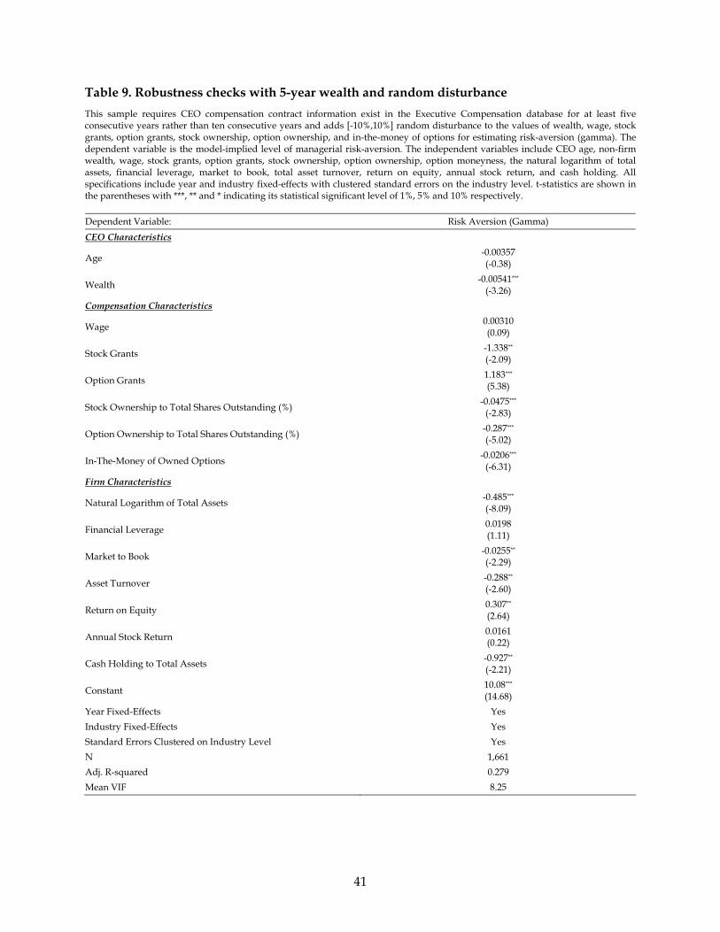
41

Table 9. Robustness checks with 5-year wealth and random disturbance

This sample requires CEO compensation contract information exist in the Executive Compensation database for at least five consecutive years rather than ten consecutive years and adds [-10%,10%] random disturbance to the values of wealth, wage, stock grants, option grants, stock ownership, option ownership, and in-the-money of options for estimating risk-aversion (gamma). The dependent variable is the model-implied level of managerial risk-aversion. The independent variables include CEO age, non-firm wealth, wage, stock grants, option grants, stock ownership, option ownership, option moneyness, the natural logarithm of total assets, financial leverage, market to book, total asset turnover, return on equity, annual stock return, and cash holding. All specifications include year and industry fixed-effects with clustered standard errors on the industry level. t-statistics are shown in the parentheses with ***, ** and * indicating its statistical significant level of 1%, 5% and 10% respectively. Dependent Variable: Risk Aversion (Gamma)

CEO Characteristics

Age -0.00357 (-0.38)

Wealth -0.00541***

(-3.26)

Compensation Characteristics

Wage 0.00310 (0.09)

Stock Grants -1.338** (-2.09)

Option Grants 1.183*** (5.38)

Stock Ownership to Total Shares Outstanding (%) -0.0475***

(-2.83)

Option Ownership to Total Shares Outstanding (%) -0.287*** (-5.02)

In-The-Money of Owned Options -0.0206***

(-6.31)

Firm Characteristics

Natural Logarithm of Total Assets -0.485*** (-8.09)

Financial Leverage 0.0198 (1.11)

Market to Book -0.0255** (-2.29)

Asset Turnover -0.288** (-2.60)

Return on Equity 0.307** (2.64)

Annual Stock Return 0.0161 (0.22)

Cash Holding to Total Assets -0.927** (-2.21)

Constant 10.08*** (14.68)

Year Fixed-Effects Yes

Industry Fixed-Effects Yes

Standard Errors Clustered on Industry Level Yes

N 1,661

Adj. R-squared 0.279

Mean VIF 8.25

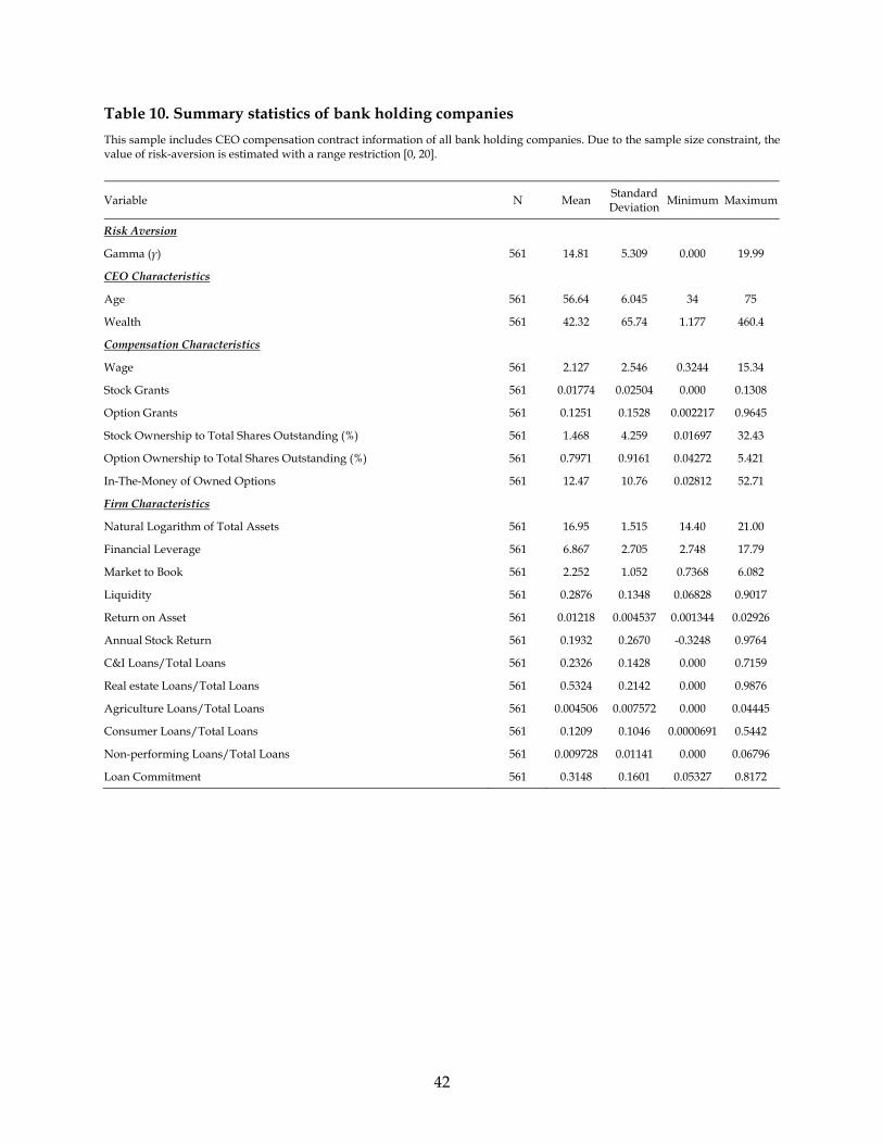
42

Table 10. Summary statistics of bank holding companies

This sample includes CEO compensation contract information of all bank holding companies. Due to the sample size constraint, the value of risk-aversion is estimated with a range restriction [0, 20].

Variable N Mean Standard Deviation

Minimum Maximum

Risk Aversion

Gamma (γ) 561 14.81 5.309 0.000 19.99

CEO Characteristics

Age 561 56.64 6.045 34 75

Wealth 561 42.32 65.74 1.177 460.4

Compensation Characteristics

Wage 561 2.127 2.546 0.3244 15.34

Stock Grants 561 0.01774 0.02504 0.000 0.1308

Option Grants 561 0.1251 0.1528 0.002217 0.9645

Stock Ownership to Total Shares Outstanding (%) 561 1.468 4.259 0.01697 32.43

Option Ownership to Total Shares Outstanding (%) 561 0.7971 0.9161 0.04272 5.421

In-The-Money of Owned Options 561 12.47 10.76 0.02812 52.71

Firm Characteristics

Natural Logarithm of Total Assets 561 16.95 1.515 14.40 21.00

Financial Leverage 561 6.867 2.705 2.748 17.79

Market to Book 561 2.252 1.052 0.7368 6.082

Liquidity 561 0.2876 0.1348 0.06828 0.9017

Return on Asset 561 0.01218 0.004537 0.001344 0.02926

Annual Stock Return 561 0.1932 0.2670 -0.3248 0.9764

C&I Loans/Total Loans 561 0.2326 0.1428 0.000 0.7159

Real estate Loans/Total Loans 561 0.5324 0.2142 0.000 0.9876

Agriculture Loans/Total Loans 561 0.004506 0.007572 0.000 0.04445

Consumer Loans/Total Loans 561 0.1209 0.1046 0.0000691 0.5442

Non-performing Loans/Total Loans 561 0.009728 0.01141 0.000 0.06796

Loan Commitment 561 0.3148 0.1601 0.05327 0.8172

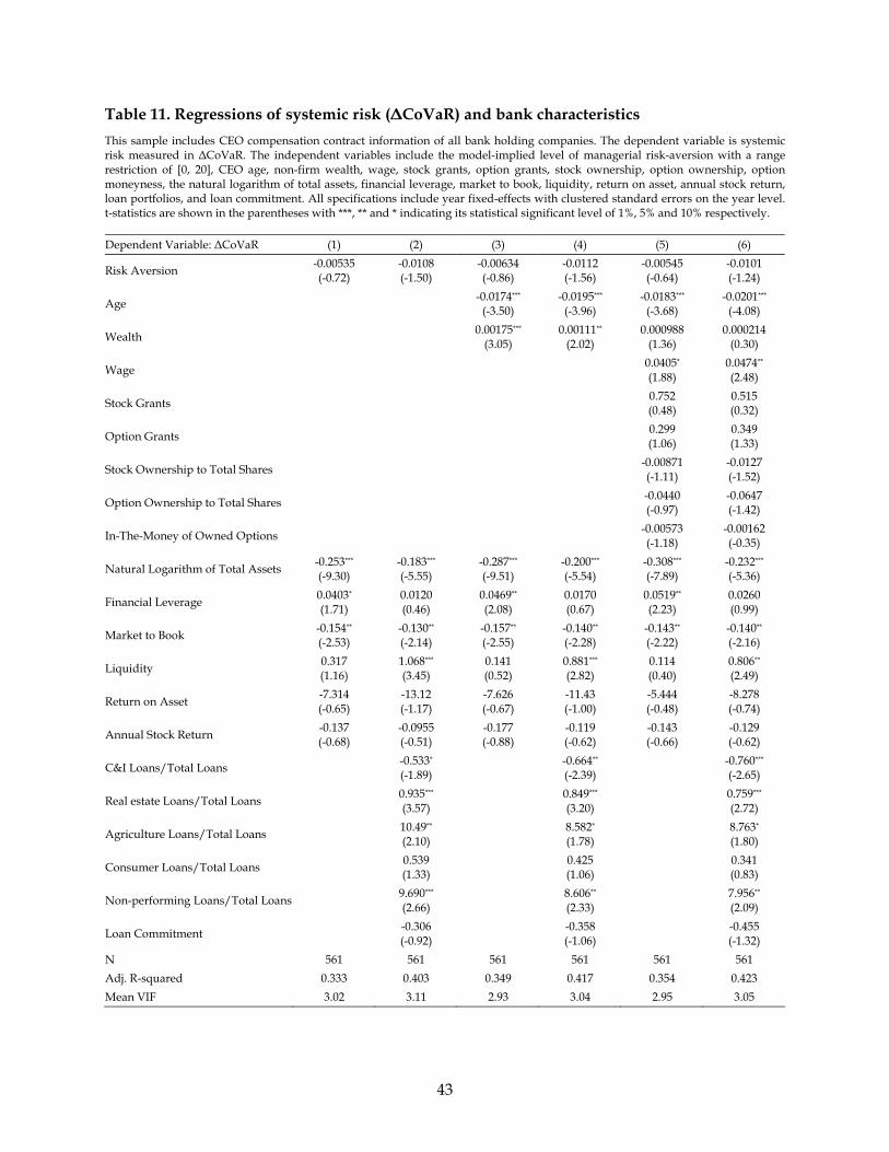
43

Table 11. Regressions of systemic risk (ΔCoVaR) and bank characteristics This sample includes CEO compensation contract information of all bank holding companies. The dependent variable is systemic risk measured in ΔCoVaR. The independent variables include the model-implied level of managerial risk-aversion with a range restriction of [0, 20], CEO age, non-firm wealth, wage, stock grants, option grants, stock ownership, option ownership, option moneyness, the natural logarithm of total assets, financial leverage, market to book, liquidity, return on asset, annual stock return, loan portfolios, and loan commitment. All specifications include year fixed-effects with clustered standard errors on the year level. t-statistics are shown in the parentheses with ***, ** and * indicating its statistical significant level of 1%, 5% and 10% respectively. Dependent Variable: ΔCoVaR (1) (2) (3) (4) (5) (6)

Risk Aversion -0.00535 (-0.72)

-0.0108 (-1.50)

-0.00634 (-0.86)

-0.0112 (-1.56)

-0.00545 (-0.64)

-0.0101 (-1.24)

Age

-0.0174*** (-3.50)

-0.0195*** (-3.96)

-0.0183*** (-3.68)

-0.0201*** (-4.08)

Wealth

0.00175*** (3.05)

0.00111** (2.02)

0.000988 (1.36)

0.000214 (0.30)

Wage

0.0405* (1.88)

0.0474** (2.48)

Stock Grants

0.752 (0.48)

0.515 (0.32)

Option Grants

0.299 (1.06)

0.349 (1.33)

Stock Ownership to Total Shares

-0.00871 (-1.11)

-0.0127 (-1.52)

Option Ownership to Total Shares

-0.0440 (-0.97)

-0.0647 (-1.42)

In-The-Money of Owned Options

-0.00573 (-1.18)

-0.00162 (-0.35)

Natural Logarithm of Total Assets -0.253*** (-9.30)

-0.183*** (-5.55)

-0.287*** (-9.51)

-0.200*** (-5.54)

-0.308*** (-7.89)

-0.232*** (-5.36)

Financial Leverage 0.0403* (1.71)

0.0120 (0.46)

0.0469** (2.08)

0.0170 (0.67)

0.0519** (2.23)

0.0260 (0.99)

Market to Book -0.154** (-2.53)

-0.130** (-2.14)

-0.157** (-2.55)

-0.140** (-2.28)

-0.143** (-2.22)

-0.140** (-2.16)

Liquidity 0.317 (1.16)

1.068*** (3.45)

0.141 (0.52)

0.881*** (2.82)

0.114 (0.40)

0.806** (2.49)

Return on Asset -7.314 (-0.65)

-13.12 (-1.17)

-7.626 (-0.67)

-11.43 (-1.00)

-5.444 (-0.48)

-8.278 (-0.74)

Annual Stock Return -0.137 (-0.68)

-0.0955 (-0.51)

-0.177 (-0.88)

-0.119 (-0.62)

-0.143 (-0.66)

-0.129 (-0.62)

C&I Loans/Total Loans

-0.533* (-1.89)

-0.664** (-2.39)

-0.760*** (-2.65)

Real estate Loans/Total Loans

0.935*** (3.57)

0.849*** (3.20)

0.759*** (2.72)

Agriculture Loans/Total Loans

10.49** (2.10)

8.582* (1.78)

8.763* (1.80)

Consumer Loans/Total Loans

0.539 (1.33)

0.425 (1.06)

0.341 (0.83)

Non-performing Loans/Total Loans

9.690*** (2.66)

8.606** (2.33)

7.956** (2.09)

Loan Commitment

-0.306 (-0.92)

-0.358 (-1.06)

-0.455 (-1.32)

N 561 561 561 561 561 561

Adj. R-squared 0.333 0.403 0.349 0.417 0.354 0.423

Mean VIF 3.02 3.11 2.93 3.04 2.95 3.05

44

Table 12. Regressions of systemic risk (SES) and bank characterstics This sample includes CEO compensation contract information of all bank holding companies. The dependent variable is systemic risk measured in SES. The independent variables include the model-implied level of managerial risk-aversion with a range restriction of [0, 20], CEO age, non-firm wealth, wage, stock grants, option grants, stock ownership, option ownership, option moneyness, the natural logarithm of total assets, financial leverage, market to book, liquidity, return on asset, annual stock return, loan portfolios, and loan commitment. All specifications include year fixed-effects with clustered standard errors on the year level. t-statistics are shown in the parentheses with ***, ** and * indicating its statistical significant level of 1%, 5% and 10% respectively. Dependent Variable: SES (1) (2) (3) (4) (5) (6)

Risk Aversion -0.00518 (-0.67)

-0.00552 (-0.68)

-0.00358 (-0.46)

-0.00389 (-0.48)

-0.00344 (-0.44)

-0.00482 (-0.56)

Age

-0.0110 (-1.65)

-0.0111* (-2.01)

-0.00711 (-1.16)

-0.00853 (-1.70)

Wealth

-0.00190** (-2.59)

-0.00195*** (-2.91)

-0.00216** (-2.19)

-0.00253*** (-2.88)

Wage

0.00376 (0.16)

0.0171 (0.75)

Stock Grants

-2.301 (-1.07)

-2.106 (-0.85)

Option Grants

0.209 (0.53)

0.286 (0.65)

Stock Ownership to Total Shares

-0.0373** (-2.24)

-0.0289* (-1.88)

Option Ownership to Total Shares

0.0205 (0.38)

-0.00520 (-0.09)

In-The-Money of Owned Options

0.00693 (1.55)

0.00928* (1.99)

Natural Logarithm of Total Assets -0.0632 (-1.07)

-0.0109 (-0.19)

-0.0127 (-0.20)

0.0424 (0.71)

-0.0432 (-0.59)

0.00558 (0.08)

Financial Leverage -0.111*** (-3.94)

-0.0896*** (-3.37)

-0.108*** (-3.78)

-0.0913*** (-3.43)

-0.0895*** (-2.98)

-0.0780** (-2.77)

Market to Book -0.455*** (-4.20)

-0.381*** (-4.66)

-0.443*** (-4.48)

-0.371*** (-4.87)

-0.433*** (-4.81)

-0.385*** (-4.85)

Liquidity -0.0115 (-0.03)

0.543 (1.11)

-0.0508 (-0.12)

0.549 (1.11)

-0.186 (-0.45)

0.355 (0.73)

Return on Asset 31.80* (1.77)

33.01* (1.87)

37.17** (2.11)

37.86** (2.18)

39.57** (2.35)

40.29** (2.43)

Annual Stock Return 0.0102 (0.02)

0.100 (0.24)

0.0679 (0.15)

0.155 (0.37)

-0.0519 (-0.12)

0.0121 (0.03)

C&I Loans/Total Loans

1.101** (2.63)

1.013** (2.56)

0.750* (1.89)

Real estate Loans/Total Loans

1.627*** (2.99)

1.690*** (3.18)

1.576*** (3.28)

Agriculture Loans/Total Loans

-2.023 (-0.39)

-3.584 (-0.77)

-2.208 (-0.51)

Consumer Loans/Total Loans

2.206*** (4.24)

2.216*** (4.18)

2.024*** (4.07)

Non-performing Loans/Total Loans

-16.36** (-2.59)

-14.66** (-2.46)

-13.37** (-2.31)

Loan Commitment

0.0411 (0.07)

0.0855 (0.15)

0.106 (0.19)

N 561 561 561 561 561 561

Adj. R-squared 0.694 0.710 0.698 0.714 0.703 0.717

Mean VIF 3.02 3.11 2.93 3.04 2.95 3.05

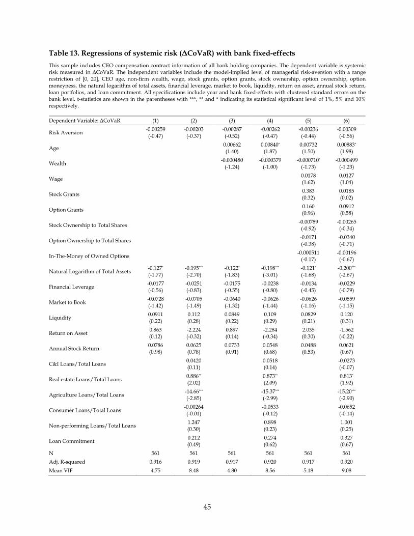
45

Table 13. Regressions of systemic risk (ΔCoVaR) with bank fixed-effects This sample includes CEO compensation contract information of all bank holding companies. The dependent variable is systemic risk measured in ΔCoVaR. The independent variables include the model-implied level of managerial risk-aversion with a range restriction of [0, 20], CEO age, non-firm wealth, wage, stock grants, option grants, stock ownership, option ownership, option moneyness, the natural logarithm of total assets, financial leverage, market to book, liquidity, return on asset, annual stock return, loan portfolios, and loan commitment. All specifications include year and bank fixed-effects with clustered standard errors on the bank level. t-statistics are shown in the parentheses with ***, ** and * indicating its statistical significant level of 1%, 5% and 10% respectively. Dependent Variable: ΔCoVaR (1) (2) (3) (4) (5) (6)

Risk Aversion -0.00259 (-0.47)

-0.00203 (-0.37)

-0.00287 (-0.52)

-0.00262 (-0.47)

-0.00236 (-0.44)

-0.00309 (-0.56)

Age

0.00662 (1.40)

0.00840* (1.87)

0.00732 (1.50)

0.00883* (1.98)

Wealth

-0.000480 (-1.24)

-0.000379 (-1.00)

-0.000710* (-1.73)

-0.000499 (-1.23)

Wage

0.0178 (1.62)

0.0127 (1.04)

Stock Grants

0.383 (0.32)

0.0185 (0.02)

Option Grants

0.160 (0.96)

0.0912 (0.58)

Stock Ownership to Total Shares

-0.00789 (-0.92)

-0.00265 (-0.34)

Option Ownership to Total Shares

-0.0171 (-0.38)

-0.0340 (-0.71)

In-The-Money of Owned Options

-0.000511 (-0.17)

-0.00196 (-0.67)

Natural Logarithm of Total Assets -0.127* (-1.77)

-0.195*** (-2.70)

-0.122* (-1.83)

-0.198*** (-3.01)

-0.121* (-1.68)

-0.200*** (-2.67)

Financial Leverage -0.0177 (-0.56)

-0.0251 (-0.83)

-0.0175 (-0.55)

-0.0238 (-0.80)

-0.0134 (-0.45)

-0.0229 (-0.79)

Market to Book -0.0728 (-1.42)

-0.0705 (-1.49)

-0.0640 (-1.32)

-0.0626 (-1.44)

-0.0626 (-1.16)

-0.0559 (-1.15)

Liquidity 0.0911 (0.22)

0.112 (0.28)

0.0849 (0.22)

0.109 (0.29)

0.0829 (0.21)

0.120 (0.31)

Return on Asset 0.863 (0.12)

-2.224 (-0.32)

0.897 (0.14)

-2.284 (-0.34)

2.035 (0.30)

-1.562 (-0.22)

Annual Stock Return 0.0786 (0.98)

0.0625 (0.78)

0.0733 (0.91)

0.0548 (0.68)

0.0488 (0.53)

0.0621 (0.67)

C&I Loans/Total Loans

0.0420 (0.11)

0.0518 (0.14)

-0.0273 (-0.07)

Real estate Loans/Total Loans

0.886** (2.02)

0.873** (2.09)

0.813* (1.92)

Agriculture Loans/Total Loans

-14.66*** (-2.85)

-15.37*** (-2.99)

-15.20*** (-2.90)

Consumer Loans/Total Loans

-0.00264 (-0.01)

-0.0533 (-0.12)

-0.0652 (-0.14)

Non-performing Loans/Total Loans

1.247 (0.30)

0.898 (0.23)

1.001 (0.25)

Loan Commitment

0.212 (0.49)

0.274 (0.62)

0.327 (0.67)

N 561 561 561 561 561 561

Adj. R-squared 0.916 0.919 0.917 0.920 0.917 0.920

Mean VIF 4.75 8.48 4.80 8.56 5.18 9.08

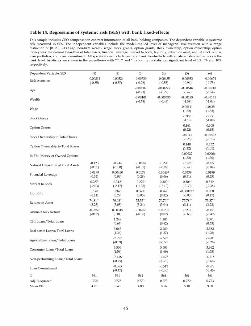
46

Table 14. Regressions of systemic risk (SES) with bank fixed-effects This sample includes CEO compensation contract information of all bank holding companies. The dependent variable is systemic risk measured in SES. The independent variables include the model-implied level of managerial risk-aversion with a range restriction of [0, 20], CEO age, non-firm wealth, wage, stock grants, option grants, stock ownership, option ownership, option moneyness, the natural logarithm of total assets, financial leverage, market to book, liquidity, return on asset, annual stock return, loan portfolios, and loan commitment. All specifications include year and bank fixed-effects with clustered standard errors on the bank level. t-statistics are shown in the parentheses with ***, ** and * indicating its statistical significant level of 1%, 5% and 10% respectively. Dependent Variable: SES (1) (2) (3) (4) (5) (6)

Risk Aversion -0.00811 (-0.85)

-0.00524 (-0.57)

-0.00730 (-0.76)

-0.00485 (-0.53)

-0.00933 (-0.94)

-0.00674 (-0.75)

Age

-0.00302 (-0.21)

-0.00293 (-0.22)

-0.00646 (-0.47)

-0.00718 (-0.54)

Wealth

-0.00101 (-0.78)

-0.000555 (-0.46)

-0.00185 (-1.38)

-0.00131 (-1.04)

Wage

0.0511* (1.72)

0.0425 (1.33)

Stock Grants

-3.985 (-1.18)

-3.533 (-1.09)

Option Grants

0.161 (0.22)

0.108 (0.15)

Stock Ownership to Total Shares

-0.0141 (-0.26)

-0.00592 (-0.13)

Option Ownership to Total Shares

0.148 (1.12)

0.132 (1.01)

In-The-Money of Owned Options

0.00922 (1.32)

0.00966 (1.30)

Natural Logarithm of Total Assets -0.123 (-0.51)

-0.244 (-1.00)

-0.0884 (-0.37)

-0.220 (-0.92)

-0.123 (-0.47)

-0.227 (-0.84)

Financial Leverage 0.0199 (0.32)

0.00460 (0.06)

0.0176 (0.28)

0.00407 (0.06)

0.0339 (0.51)

0.0189 (0.25)

Market to Book -0.287** (-2.03)

-0.312** (-2.17)

-0.270** (-1.98)

-0.302** (-2.12)

-0.304** (-2.30)

-0.340** (-2.38)

Liquidity 0.170 (0.14)

0.346 (0.29)

0.0605 (0.05)

0.262 (0.22)

-0.000277 (-0.00)

0.208 (0.17)

Return on Asset 74.81*** (3.23)

70.08*** (3.03)

75.55*** (3.24)

70.70*** (3.04)

77.78*** (3.41)

73.37*** (3.23)

Annual Stock Return -0.0259 (-0.07)

0.00345 (0.01)

-0.0207 (-0.06)

0.00730 (0.02)

-0.212 (-0.65)

-0.156 (-0.49)

C&I Loans/Total Loans

1.248 (0.63)

1.205 (0.62)

1.081 (0.55)

Real estate Loans/Total Loans

3.067 (1.36)

2.980 (1.37)

2.582 (1.26)

Agriculture Loans/Total Loans

-7.957 (-0.59)

-7.527 (-0.56)

-3.603 (-0.26)

Consumer Loans/Total Loans

3.506 (1.59)

3.503 (1.60)

3.362 (1.55)

Non-performing Loans/Total Loans

-7.438 (-0.75)

-7.427 (-0.76)

-6.215 (-0.66)

Loan Commitment

-0.563 (-0.47)

-0.511 (-0.40)

-0.575 (-0.46)

N 561 561 561 561 561 561

Adj. R-squared 0.770 0.773 0.770 0.773 0.772 0.773

Mean VIF 4.75 8.48 4.80 8.56 5.18 9.08

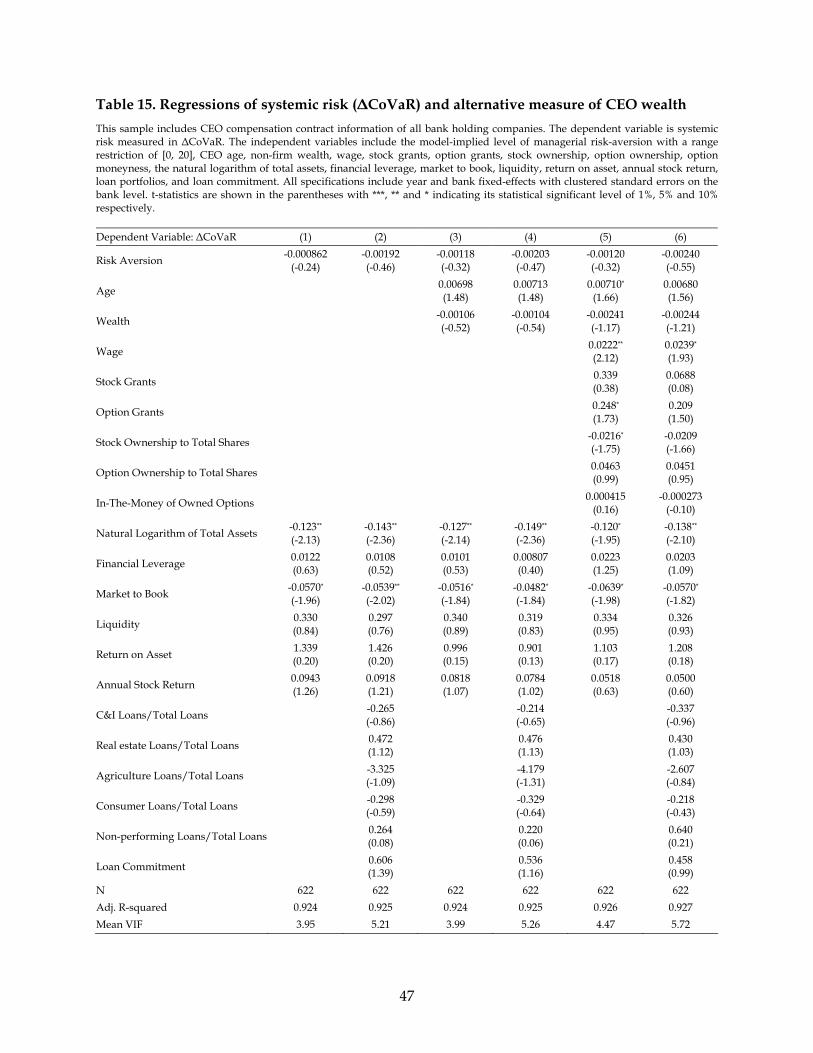
47

Table 15. Regressions of systemic risk (ΔCoVaR) and alternative measure of CEO wealth This sample includes CEO compensation contract information of all bank holding companies. The dependent variable is systemic risk measured in ΔCoVaR. The independent variables include the model-implied level of managerial risk-aversion with a range restriction of [0, 20], CEO age, non-firm wealth, wage, stock grants, option grants, stock ownership, option ownership, option moneyness, the natural logarithm of total assets, financial leverage, market to book, liquidity, return on asset, annual stock return, loan portfolios, and loan commitment. All specifications include year and bank fixed-effects with clustered standard errors on the bank level. t-statistics are shown in the parentheses with ***, ** and * indicating its statistical significant level of 1%, 5% and 10% respectively. Dependent Variable: ΔCoVaR (1) (2) (3) (4) (5) (6)

Risk Aversion -0.000862

(-0.24) -0.00192 (-0.46)

-0.00118 (-0.32)

-0.00203 (-0.47)

-0.00120 (-0.32)

-0.00240 (-0.55)

Age

0.00698 (1.48)

0.00713 (1.48)

0.00710* (1.66)

0.00680 (1.56)

Wealth

-0.00106 (-0.52)

-0.00104 (-0.54)

-0.00241 (-1.17)

-0.00244 (-1.21)

Wage

0.0222** (2.12)

0.0239* (1.93)

Stock Grants

0.339 (0.38)

0.0688 (0.08)

Option Grants

0.248* (1.73)

0.209 (1.50)

Stock Ownership to Total Shares

-0.0216* (-1.75)

-0.0209 (-1.66)

Option Ownership to Total Shares

0.0463 (0.99)

0.0451 (0.95)

In-The-Money of Owned Options

0.000415 (0.16)

-0.000273 (-0.10)

Natural Logarithm of Total Assets -0.123** (-2.13)

-0.143** (-2.36)

-0.127** (-2.14)

-0.149** (-2.36)

-0.120* (-1.95)

-0.138** (-2.10)

Financial Leverage 0.0122 (0.63)

0.0108 (0.52)

0.0101 (0.53)

0.00807 (0.40)

0.0223 (1.25)

0.0203 (1.09)

Market to Book -0.0570* (-1.96)

-0.0539** (-2.02)

-0.0516* (-1.84)

-0.0482* (-1.84)

-0.0639* (-1.98)

-0.0570* (-1.82)

Liquidity 0.330 (0.84)

0.297 (0.76)

0.340 (0.89)

0.319 (0.83)

0.334 (0.95)

0.326 (0.93)

Return on Asset 1.339 (0.20)

1.426 (0.20)

0.996 (0.15)

0.901 (0.13)

1.103 (0.17)

1.208 (0.18)

Annual Stock Return 0.0943 (1.26)

0.0918 (1.21)

0.0818 (1.07)

0.0784 (1.02)

0.0518 (0.63)

0.0500 (0.60)

C&I Loans/Total Loans

-0.265 (-0.86)

-0.214 (-0.65)

-0.337 (-0.96)

Real estate Loans/Total Loans

0.472 (1.12)

0.476 (1.13)

0.430 (1.03)

Agriculture Loans/Total Loans

-3.325 (-1.09)

-4.179 (-1.31)

-2.607 (-0.84)

Consumer Loans/Total Loans

-0.298 (-0.59)

-0.329 (-0.64)

-0.218 (-0.43)

Non-performing Loans/Total Loans

0.264 (0.08)

0.220 (0.06)

0.640 (0.21)

Loan Commitment

0.606 (1.39)

0.536 (1.16)

0.458 (0.99)

N 622 622 622 622 622 622

Adj. R-squared 0.924 0.925 0.924 0.925 0.926 0.927

Mean VIF 3.95 5.21 3.99 5.26 4.47 5.72

48

Table 16. Regressions of systemic risk (SES) and alternative measure of CEO wealth This sample includes CEO compensation contract information of all bank holding companies. The dependent variable is systemic risk measured in SES. The independent variables include the model-implied level of managerial risk-aversion with a range restriction of [0, 20], CEO age, non-firm wealth, wage, stock grants, option grants, stock ownership, option ownership, option moneyness, the natural logarithm of total assets, financial leverage, market to book, liquidity, return on asset, annual stock return, loan portfolios, and loan commitment. All specifications include year and bank fixed-effects with clustered standard errors on the bank level. t-statistics are shown in the parentheses with ***, ** and * indicating its statistical significant level of 1%, 5% and 10% respectively. Dependent Variable: SES (1) (2) (3) (4) (5) (6)

Risk Aversion 0.00208 (0.21)

0.000290 (0.03)

0.00287 (0.29)

0.000464 (0.05)

-0.00113 (-0.10)

-0.00364 (-0.35)

Age

-0.0184 (-1.31)

-0.0215 (-1.39)

-0.0223 (-1.50)

-0.0250 (-1.54)

Wealth

0.00259 (0.51)

0.00262 (0.54)

0.00188 (0.34)

0.00150 (0.28)

Wage

0.0154 (0.36)

0.0243 (0.53)

Stock Grants

-2.167 (-0.90)

-2.073 (-0.87)

Option Grants

-0.389 (-0.82)

-0.399 (-0.81)

Stock Ownership to Total Shares

0.0795*** (3.89)

0.0724*** (3.46)

Option Ownership to Total Shares

0.0263 (0.23)

0.0292 (0.24)

In-The-Money of Owned Options

-0.00421 (-0.48)

-0.00376 (-0.40)

Natural Logarithm of Total Assets -0.159 (-0.87)

-0.179 (-0.85)

-0.147 (-0.73)

-0.160 (-0.69)

-0.113 (-0.51)

-0.144 (-0.57)

Financial Leverage 0.0492 (0.61)

0.0577 (0.70)

0.0548 (0.67)

0.0658 (0.79)

0.0420 (0.49)

0.0532 (0.62)

Market to Book -0.122 (-1.12)

-0.136 (-1.21)

-0.136 (-1.19)

-0.152 (-1.31)

-0.115 (-1.13)

-0.133 (-1.23)

Liquidity -0.203 (-0.20)

-0.315 (-0.29)

-0.233 (-0.24)

-0.388 (-0.37)

-0.339 (-0.33)

-0.503 (-0.45)

Return on Asset 53.26** (2.16)

52.99** (2.13)

54.18** (2.21)

54.60** (2.20)

60.06** (2.45)

60.10** (2.43)

Annual Stock Return 0.145 (0.43)

0.177 (0.52)

0.177 (0.53)

0.216 (0.63)

0.222 (0.66)

0.248 (0.72)

C&I Loans/Total Loans

-0.812 (-0.51)

-0.959 (-0.57)

-1.111 (-0.65)

Real estate Loans/Total Loans

0.393 (0.27)

0.389 (0.27)

0.349 (0.23)

Agriculture Loans/Total Loans

0.857 (0.10)

3.405 (0.38)

1.926 (0.22)

Consumer Loans/Total Loans

1.997 (1.21)

2.108 (1.28)

1.582 (0.94)

Non-performing Loans/Total Loans

-8.028 (-1.07)

-7.812 (-1.09)

-5.481 (-0.70)

Loan Commitment

0.157 (0.14)

0.373 (0.32)

0.652 (0.57)

N 622 622 622 622 622 622

Adj. R-squared 0.924 0.925 0.924 0.925 0.926 0.927

Mean VIF 3.95 5.21 3.99 5.26 4.47 5.72