1

Exercise 7: Viewshed Analysis and Introduction to 3D GIS

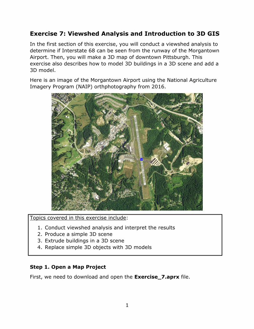
In the first section of this exercise, you will conduct a viewshed analysis to determine if Interstate 68 can be seen from the runway of the Morgantown Airport. Then, you will make a 3D map of downtown Pittsburgh. This exercise also describes how to model 3D buildings in a 3D scene and add a 3D model.

Here is an image of the Morgantown Airport using the National Agriculture Imagery Program (NAIP) orthphotography from 2016.

Topics covered in this exercise include:

1. Conduct viewshed analysis and interpret the results 2. Produce a simple 3D scene 3. Extrude buildings in a 3D scene 4. Replace simple 3D objects with 3D models

Step 1. Open a Map Project

First, we need to download and open the Exercise_7.aprx file.

2

� Download the Exercise_7 lab folder from the class webpage under Education tab on http://www.wvview.org/. All lab material is available under “Labs and Data” tab.

� Click on the “L7 Data” button to download the Exercise_7.zip file. � You will need to extract the compressed files and save it to the

location of your choosing. � Open ArcGIS Pro. This can be done by navigating to All Apps followed

by the ArcGIS Folder. Within the ArcGIS Folder, select ArcGIS Pro. Note that you can also use a Task Bar or Desktop shortcut if they are available on your machine.

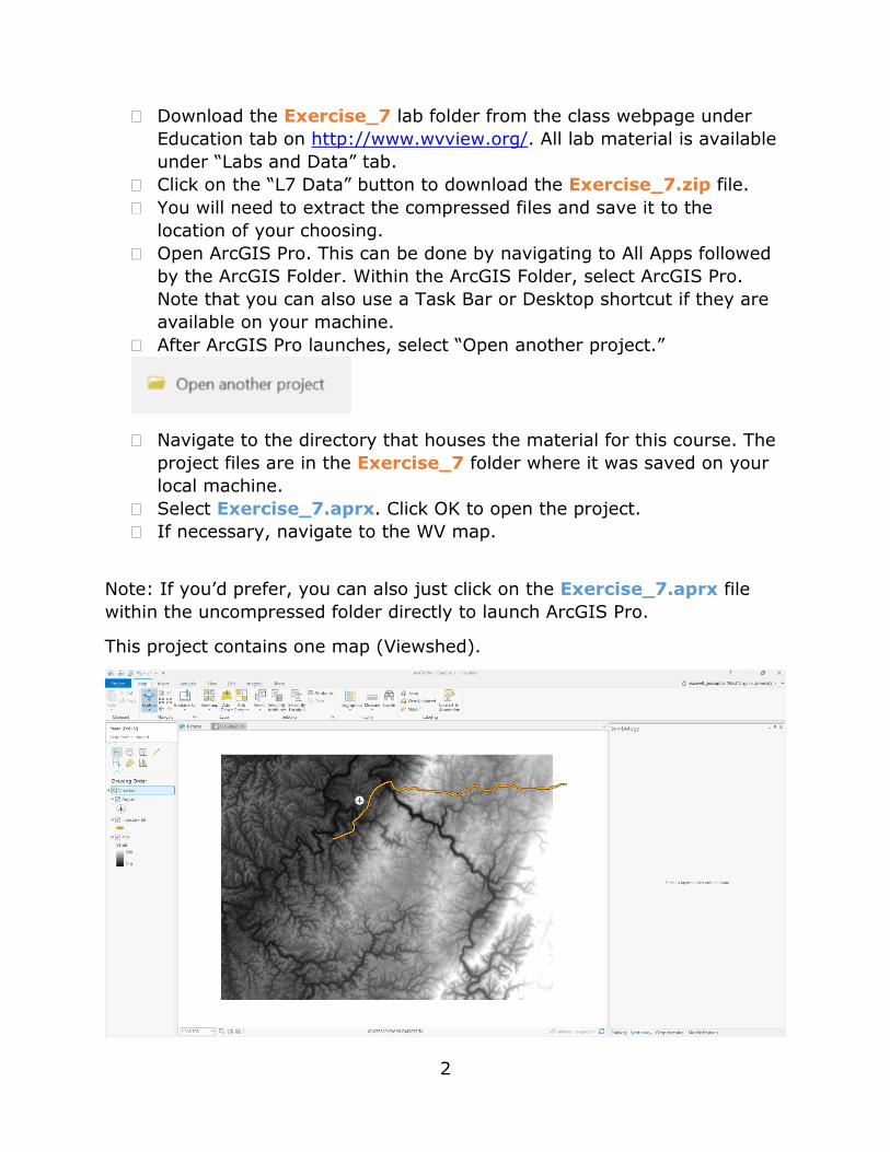
� After ArcGIS Pro launches, select “Open another project.”

� Navigate to the directory that houses the material for this course. The project files are in the Exercise_7 folder where it was saved on your local machine.

� Select Exercise_7.aprx. Click OK to open the project. � If necessary, navigate to the WV map.

Note: If you’d prefer, you can also just click on the Exercise_7.aprx file within the uncompressed folder directly to launch ArcGIS Pro.

This project contains one map (Viewshed).

3

Step 2. Setting Up the Working Environment

In this lab, you will generate some outputs. Before you begin, it is a good idea to set up the working environment. Specifically, you will set a current workspace and a scratch workspace. If you plan to perform data analysis and spatial analysis in a project, it is a good idea to set environment settings.

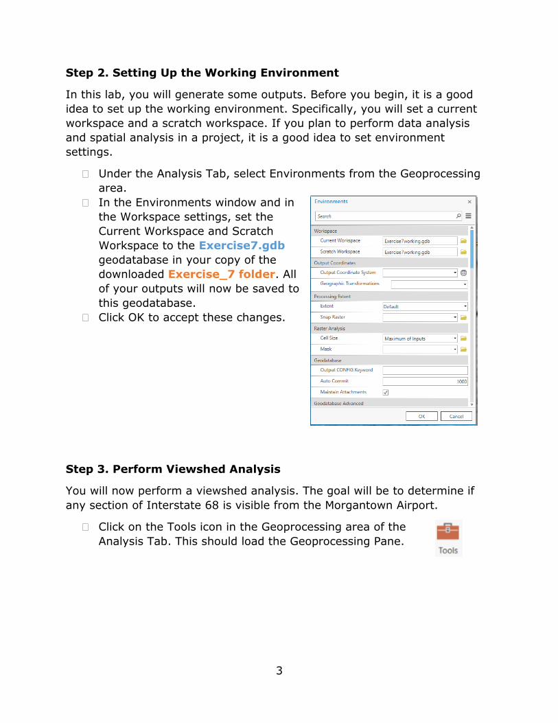
� Under the Analysis Tab, select Environments from the Geoprocessing area.

� In the Environments window and in the Workspace settings, set the Current Workspace and Scratch Workspace to the Exercise7.gdb geodatabase in your copy of the downloaded Exercise_7 folder. All of your outputs will now be saved to this geodatabase.

� Click OK to accept these changes.

Step 3. Perform Viewshed Analysis

You will now perform a viewshed analysis. The goal will be to determine if any section of Interstate 68 is visible from the Morgantown Airport.

� Click on the Tools icon in the Geoprocessing area of the Analysis Tab. This should load the Geoprocessing Pane.

4

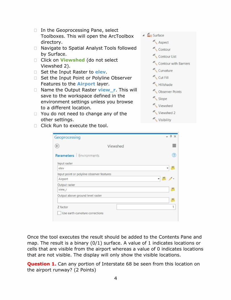
� In the Geoprocessing Pane, select Toolboxes. This will open the ArcToolbox directory.

� Navigate to Spatial Analyst Tools followed by Surface.

� Click on Viewshed (do not select Viewshed 2).

� Set the Input Raster to elev. � Set the Input Point or Polyline Observer

Features to the Airport layer. � Name the Output Raster view_r. This will

save to the workspace defined in the environment settings unless you browse to a different location.

� You do not need to change any of the other settings.

� Click Run to execute the tool.

Once the tool executes the result should be added to the Contents Pane and map. The result is a binary (0/1) surface. A value of 1 indicates locations or cells that are visible from the airport whereas a value of 0 indicates locations that are not visible. The display will only show the visible locations.

Question 1. Can any portion of Interstate 68 be seen from this location on the airport runway? (2 Points)

5

Question 2. What is one factor that could impact visibility that is not modelled using only a DEM and the Viewshed tool? (4 Points)

Question 3. In this exercise, we did not calculate an output above ground level raster. Using the tool help, explain what this output would show. (4 Points)

Question 4. Using the tool help, explain the purpose of the Z factor when conducting a viewshed analysis. (4 Points)

Step 4. Creating a 3D Scene

You will now create a simple 3D scene of downtown Pittsburgh. Before you can begin, you will need to add a new scene to the map. 3D scenes are created within scenes as opposed to maps.

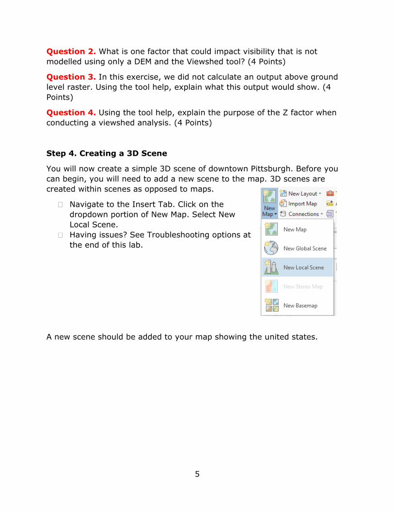
� Navigate to the Insert Tab. Click on the dropdown portion of New Map. Select New Local Scene.

� Having issues? See Troubleshooting options at the end of this lab.

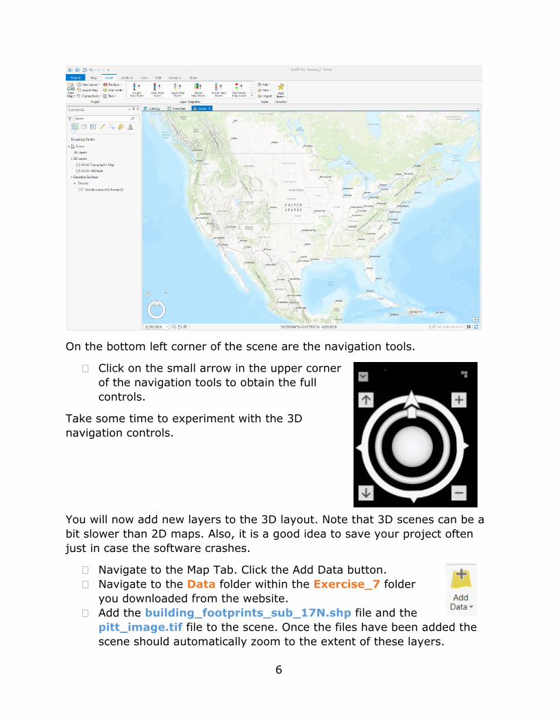
A new scene should be added to your map showing the united states.

6

On the bottom left corner of the scene are the navigation tools.

� Click on the small arrow in the upper corner of the navigation tools to obtain the full controls.

Take some time to experiment with the 3D navigation controls.

You will now add new layers to the 3D layout. Note that 3D scenes can be a bit slower than 2D maps. Also, it is a good idea to save your project often just in case the software crashes.

� Navigate to the Map Tab. Click the Add Data button. � Navigate to the Data folder within the Exercise_7 folder

you downloaded from the website. � Add the building_footprints_sub_17N.shp file and the

pitt_image.tif file to the scene. Once the files have been added the scene should automatically zoom to the extent of these layers.

7

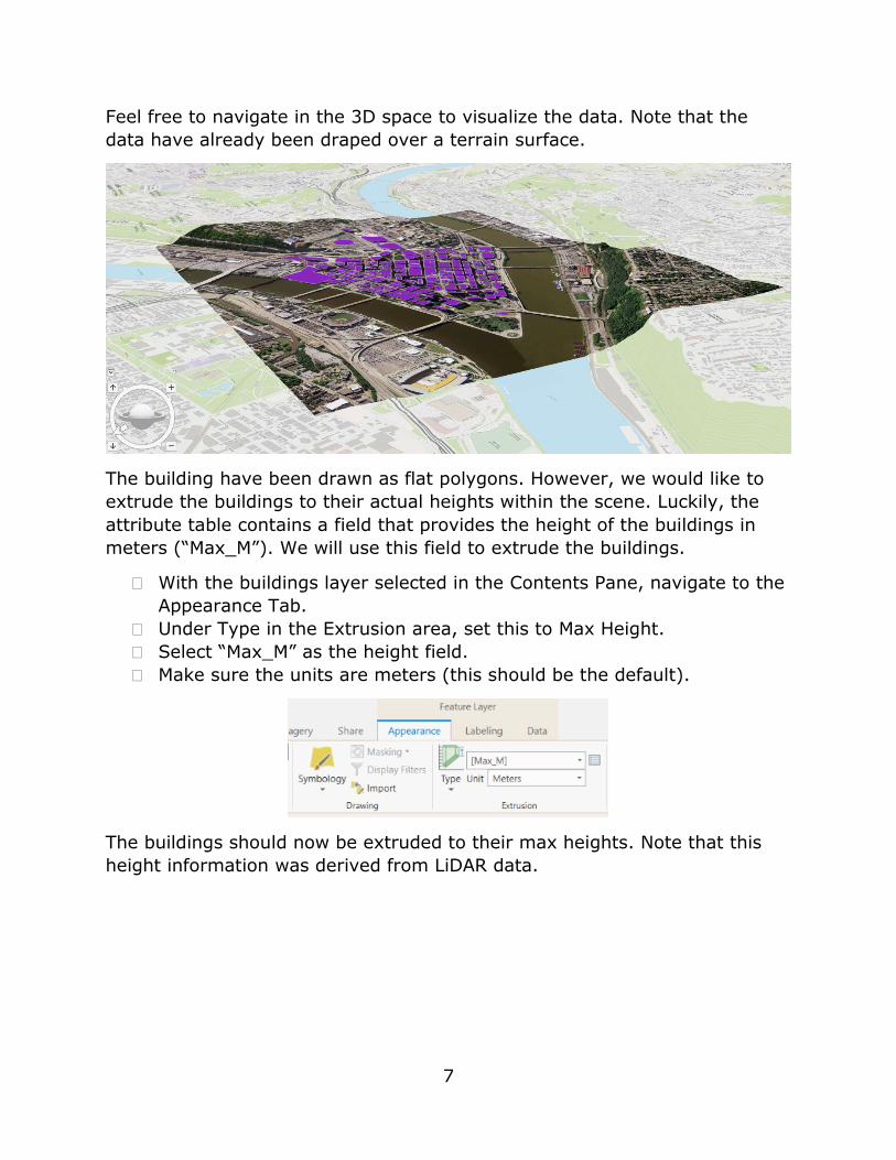
Feel free to navigate in the 3D space to visualize the data. Note that the data have already been draped over a terrain surface.

The building have been drawn as flat polygons. However, we would like to extrude the buildings to their actual heights within the scene. Luckily, the attribute table contains a field that provides the height of the buildings in meters (“Max_M”). We will use this field to extrude the buildings.

� With the buildings layer selected in the Contents Pane, navigate to the Appearance Tab.

� Under Type in the Extrusion area, set this to Max Height. � Select “Max_M” as the height field. � Make sure the units are meters (this should be the default).

The buildings should now be extruded to their max heights. Note that this height information was derived from LiDAR data.

8

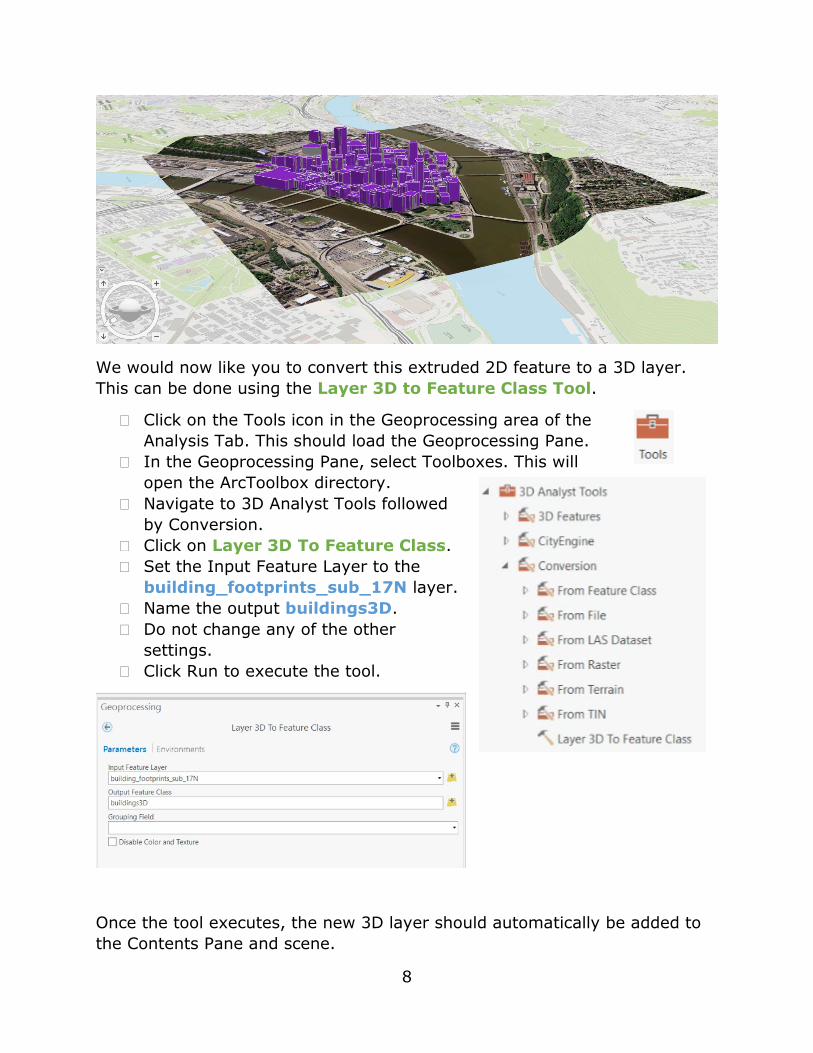
We would now like you to convert this extruded 2D feature to a 3D layer. This can be done using the Layer 3D to Feature Class Tool.

� Click on the Tools icon in the Geoprocessing area of the Analysis Tab. This should load the Geoprocessing Pane.

� In the Geoprocessing Pane, select Toolboxes. This will open the ArcToolbox directory.

� Navigate to 3D Analyst Tools followed by Conversion.

� Click on Layer 3D To Feature Class. � Set the Input Feature Layer to the

building_footprints_sub_17N layer. � Name the output buildings3D. � Do not change any of the other

settings. � Click Run to execute the tool.

Once the tool executes, the new 3D layer should automatically be added to the Contents Pane and scene.

9

� Uncheck or remove the original 2D buildings layer.

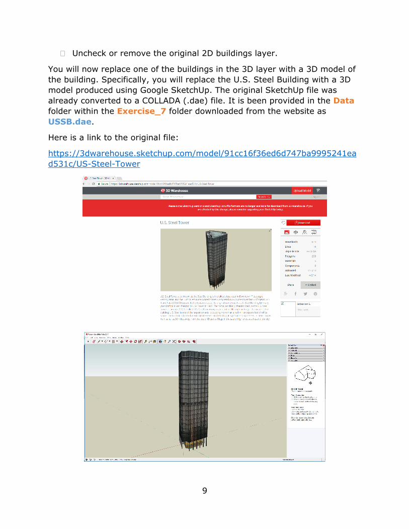
You will now replace one of the buildings in the 3D layer with a 3D model of the building. Specifically, you will replace the U.S. Steel Building with a 3D model produced using Google SketchUp. The original SketchUp file was already converted to a COLLADA (.dae) file. It is been provided in the Data folder within the Exercise_7 folder downloaded from the website as USSB.dae.

Here is a link to the original file:

https://3dwarehouse.sketchup.com/model/91cc16f36ed6d747ba9995241ead531c/US-Steel-Tower

10

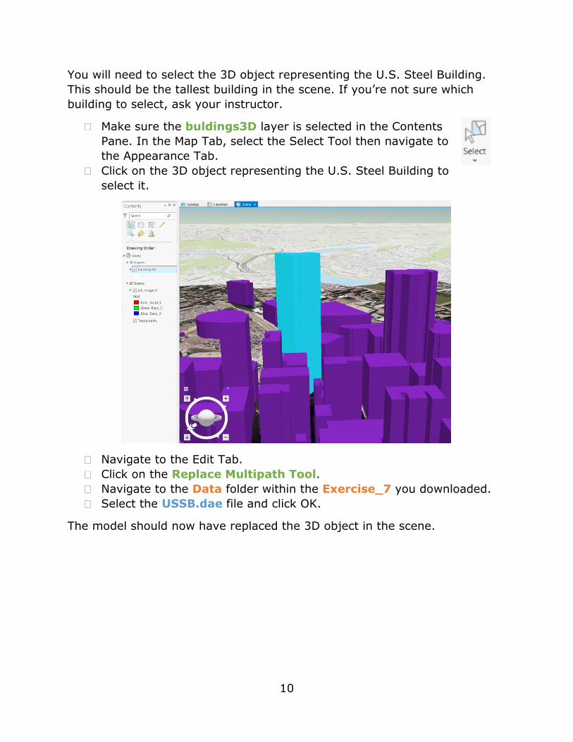
You will need to select the 3D object representing the U.S. Steel Building. This should be the tallest building in the scene. If you’re not sure which building to select, ask your instructor.

� Make sure the buldings3D layer is selected in the Contents Pane. In the Map Tab, select the Select Tool then navigate to the Appearance Tab.

� Click on the 3D object representing the U.S. Steel Building to select it.

� Navigate to the Edit Tab. � Click on the Replace Multipath Tool. � Navigate to the Data folder within the Exercise_7 you downloaded. � Select the USSB.dae file and click OK.

The model should now have replaced the 3D object in the scene.

11

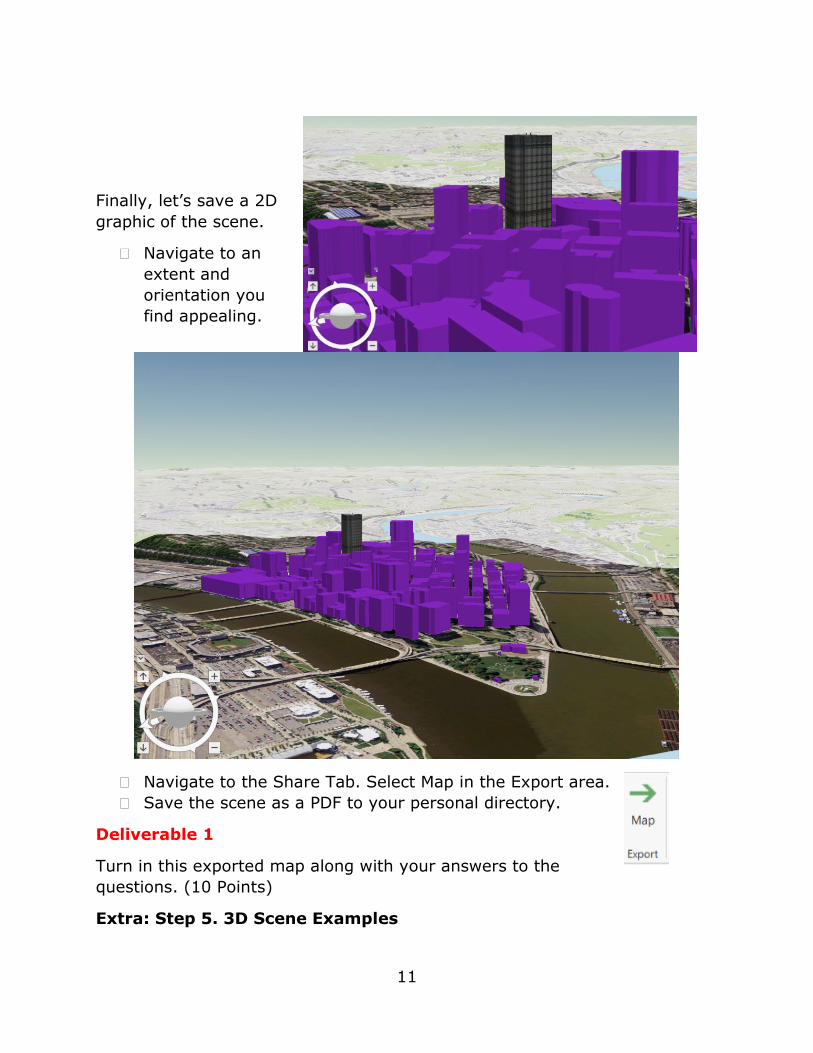
Finally, let’s save a 2D graphic of the scene.

� Navigate to an extent and orientation you find appealing.

� Navigate to the Share Tab. Select Map in the Export area. � Save the scene as a PDF to your personal directory.

Deliverable 1

Turn in this exported map along with your answers to the questions. (10 Points)

Extra: Step 5. 3D Scene Examples

12

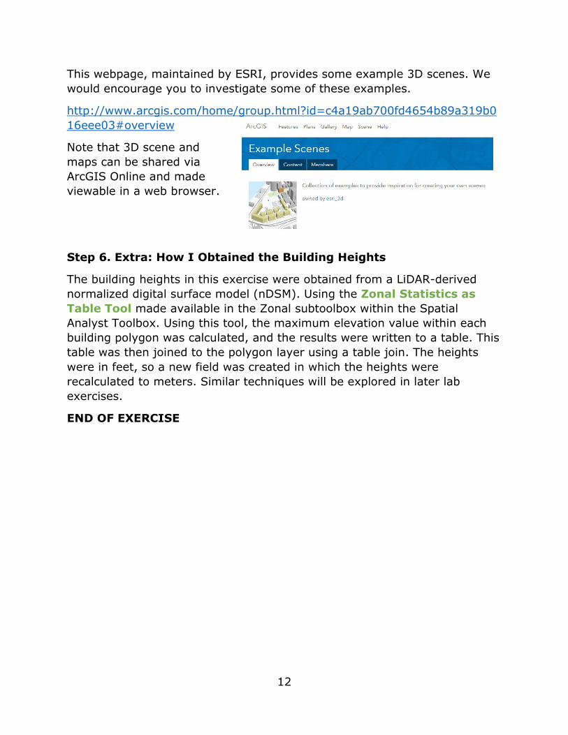
This webpage, maintained by ESRI, provides some example 3D scenes. We would encourage you to investigate some of these examples.

http://www.arcgis.com/home/group.html?id=c4a19ab700fd4654b89a319b016eee03#overview

Note that 3D scene and maps can be shared via ArcGIS Online and made viewable in a web browser.

Step 6. Extra: How I Obtained the Building Heights

The building heights in this exercise were obtained from a LiDAR-derived normalized digital surface model (nDSM). Using the Zonal Statistics as Table Tool made available in the Zonal subtoolbox within the Spatial Analyst Toolbox. Using this tool, the maximum elevation value within each building polygon was calculated, and the results were written to a table. This table was then joined to the polygon layer using a table join. The heights were in feet, so a new field was created in which the heights were recalculated to meters. Similar techniques will be explored in later lab exercises.

END OF EXERCISE

13

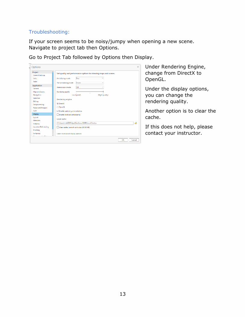
Troubleshooting:

If your screen seems to be noisy/jumpy when opening a new scene. Navigate to project tab then Options.

Go to Project Tab followed by Options then Display.

Under Rendering Engine, change from DirectX to OpenGL.

Under the display options, you can change the rendering quality.

Another option is to clear the cache.

If this does not help, please contact your instructor.