Embed Size (px)
Citation preview

Exercise organisation (planned)
• 3 exercise sheets: computation examples, implementation
• All information at: http://av.dfki.de/lecture/
• Hand in exercise solutions, if you want feedback
• Schedule:
• Solutions will be discussed in exercise sessions
Sheet out (Monday)
Lectures (Monday)
Solution in (Tuesday)
Session (Thursday, 14:00-15:30)
04.06. 04.06., 11.06. 12.06. 14.06.
18.06. 18.06., 25.06. 26.06. 28.06.
02.07 02.07., 09.07. 11.07.
16.07. (ex. session)
1

Recap: Model-based 3D tracking
Doz. G. Bleser
Prof. Stricker
Computer Vision: Object and People Tracking

3
Intrinsic camera parameters
𝑚𝑖
𝑢𝑣𝑤=𝑓𝑥 𝑠𝛼 ℎ𝑥0 𝑓𝑦 ℎ𝑦0 0 1
𝐾
𝑥𝑐𝑦𝑐𝑧𝑐
𝑥𝑝𝑦𝑝
= 𝑢/𝑤𝑣/𝑤
𝑓𝑥 =𝑓
𝑑𝑥
𝑓𝑦 =𝑓
𝑑𝑦

4
Extrinsic camera parameters and P-matrix
𝑚𝑐 = 𝑅𝑐𝑤 𝑚𝑤 − 𝑐𝑤
or 𝑚𝑐 = 𝑅𝑐𝑤𝑚𝑤 +𝑤𝑐
In matrix form:
𝑀
𝑥𝑐𝑦𝑐𝑧𝑐= 𝑅𝑐𝑤 𝑤𝑐
𝑥𝑤𝑦𝑤𝑧𝑤1
𝑥𝑝𝑦𝑝1∝ 𝑧𝑐
𝑥𝑝𝑦𝑝1= 𝐾 ∙ 𝑅𝑐𝑤 𝑤𝑐
𝑃
𝑥𝑤𝑦𝑤𝑧𝑤1
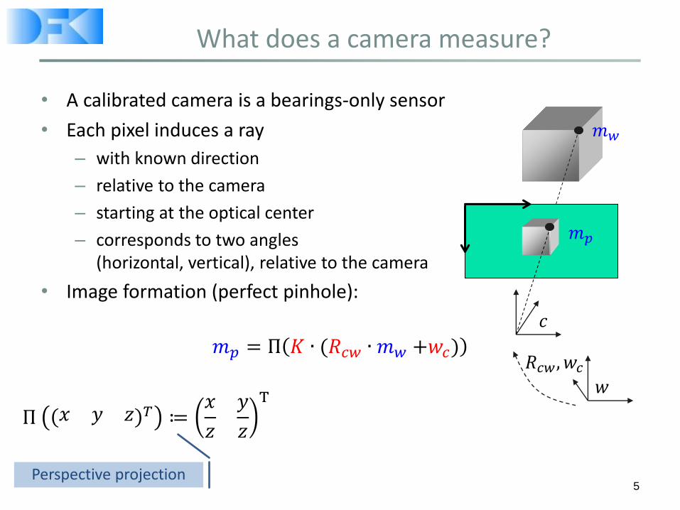
What does a camera measure?
• A calibrated camera is a bearings-only sensor
• Each pixel induces a ray
– with known direction
– relative to the camera
– starting at the optical center
– corresponds to two angles (horizontal, vertical), relative to the camera
• Image formation (perfect pinhole):
𝑚𝑝 = Π 𝐾 ∙ (𝑅𝑐𝑤 ∙ 𝑚𝑤 +𝑤𝑐)
5
𝑅𝑐𝑤, 𝑤𝑐
𝑐
𝑤
𝑚𝑤
𝑚𝑝
Perspective projection
Π 𝑥 𝑦 𝑧 𝑇 ≔𝑥
𝑧
𝑦
𝑧
T

Camera pose estimation
• Estimation of camera poses given corresponding 2D and 3D coordinates.
Camera pose
2D feature location (from image processing)
3D feature location
6

3D reconstruction (triangulation)
• Estimation of 3D points given corresponding 2D coordinates and camera poses.
Camera pose
2D feature location (from image processing)
3D feature location
7

SA-1
Camera pose estimation based on a CAD model and contours

Edge-based tracking = the „RAPiD“ algorithm [Harris, 1992]
RAPiD = Real-time Attitude and Position Determination
A. Pre-processing: compute the edge map
B. Iterate two steps: 1. data association, 2. pose update
Data association Giorgio Panin
Pose update
The RAPiD algorithm
9

B. Data association and pose computation
• The 3D edge model is projected onto the image, using the last pose.
• Control points 𝑝𝑖 are defined at regular distance for each edge 𝐸 of the model.
pi
10

B. Data association and pose computation
• An orthogonal search segment is defined at each pi
• Candiates qi,j are defined along this segment.
pi
qi,1
qi,2
11
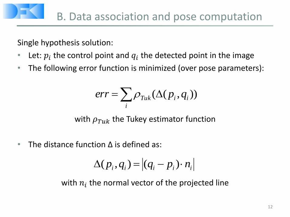
B. Data association and pose computation
Single hypothesis solution:
• Let: 𝑝𝑖 the control point and 𝑞𝑖 the detected point in the image
• The following error function is minimized (over pose parameters):
with 𝜌𝑇𝑢𝑘 the Tukey estimator function
• The distance function Δ is defined as:
with 𝑛𝑖 the normal vector of the projected line
12
i
iiTuk qperr )),((
iiiii npqqp )(),(
B. Data association and pose computation
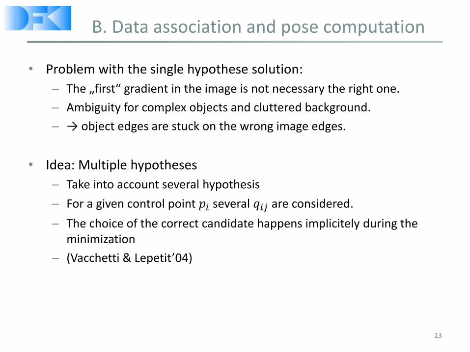
• Problem with the single hypothese solution:
– The „first“ gradient in the image is not necessary the right one.
– Ambiguity for complex objects and cluttered background.
– → object edges are stuck on the wrong image edges.
• Idea: Multiple hypotheses
– Take into account several hypothesis
– For a given control point 𝑝𝑖 several 𝑞𝑖𝑗 are considered.
– The choice of the correct candidate happens implicitely during the minimization
– (Vacchetti & Lepetit’04)
13

B. Data association and pose computation
For multiple hypothsis, we have:
• Let: 𝑝𝑖 the control points of the edge and 𝑞𝑖,𝑗 multiple potential
candidates.
• The following error function is minimized:
• The estimator function is computed for the hypothesis, which has the smallest distance to the projected point.
14
i
jiij
Tuk qperr )),(min( ,
p2
q2,1
q2,2
q2,3

B. Data association and pose computation
Summary multiple hypotheses:
• More expensive in computation, but still real-time.
• More robust!
• Ambiguities are solved through consideration of multiple candidates.
15
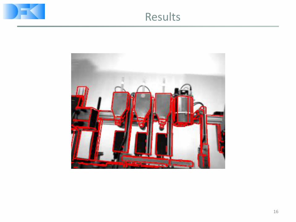
Results
16

Computer vision: object and people tracking
• Part I: Mostly image processing
• Part II: Probabilistic estimation
– Bayesian tracking framework
– Gaussian filters: (extended) Kalman filter
– Motion and measurement models (in 3D)
• Part III: Applications bringing Part I and Part II together
17

Introduction to Bayesian tracking
Doz. G. Bleser
Prof. Stricker
Computer Vision: Object and People Tracking

SA-1
What we learnt until now…
Some slides based on G. Panin, S. Thrun, K. Smith

Mostly visual data processing
• Visual modalities and natural features
• Feature tracking
• Template matching
• …
21
Object/
people tracking Modalities
Vision
Color Motion Edges Keypoints Texture
Data association
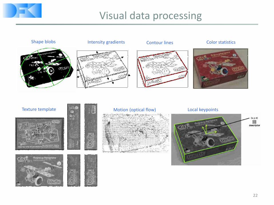
Shape blobs Intensity gradients Contour lines Color statistics
Texture template Motion (optical flow) Local keypoints
Visual data processing
22

Objects
Models
A bit about modelling
Object/
people tracking
Degrees of freedom
Appearance
Shape
Modalities
Vision Data association
23
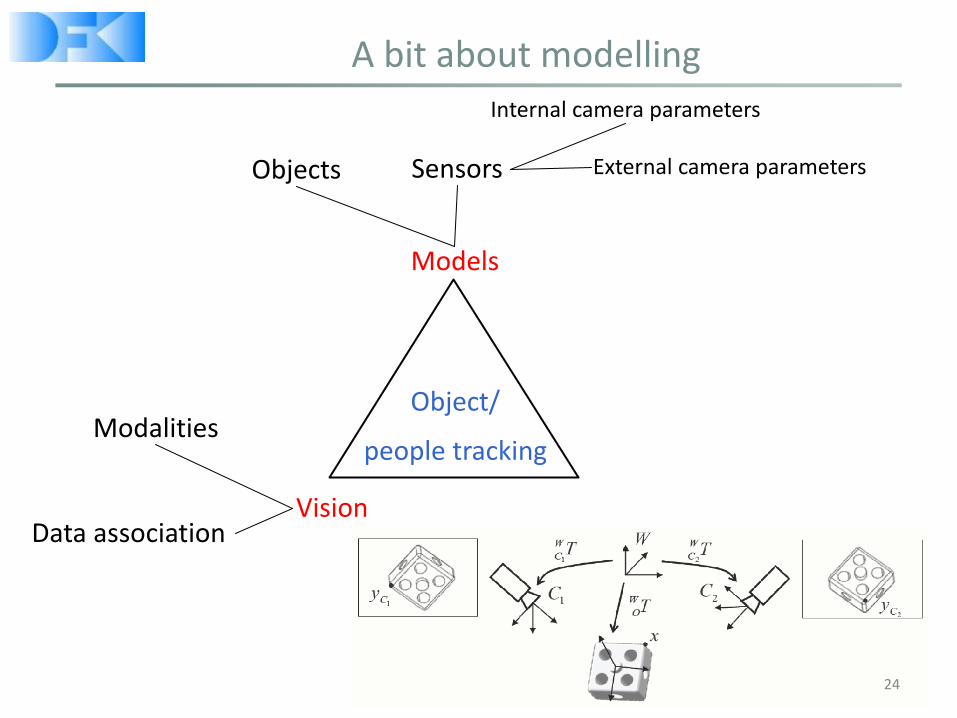
Objects Sensors
Models
A bit about modelling
Object/
people tracking
Internal camera parameters
External camera parameters
Modalities
Vision Data association
24

Objects Sensors
Models
Context
Modalities
Vision Data association
A bit about modelling
Object/
people tracking
Background modelling
25

SA-1
Object/people tracking is much more
Motivation examples…

Humanoid robot catches flying balls
27 Courtesy of U. Frese

Humanoid robot catches flying balls
• Complex tracking problem:
– Distinguish flying balls from other objects that look like balls
– Track multiple targets in reference frame of moving robot
– Predict ball trajectories for catching! Early enough!
– Move robot hand to right position
• Approach:
– Multiple hypothesis tracking
– Multiple target tracking
– Multiple sensor fusion (cameras, IMU)
– Physical model for object dynamics (constant velocity + gravity)
– Kinematic chain (robot head hand)
28
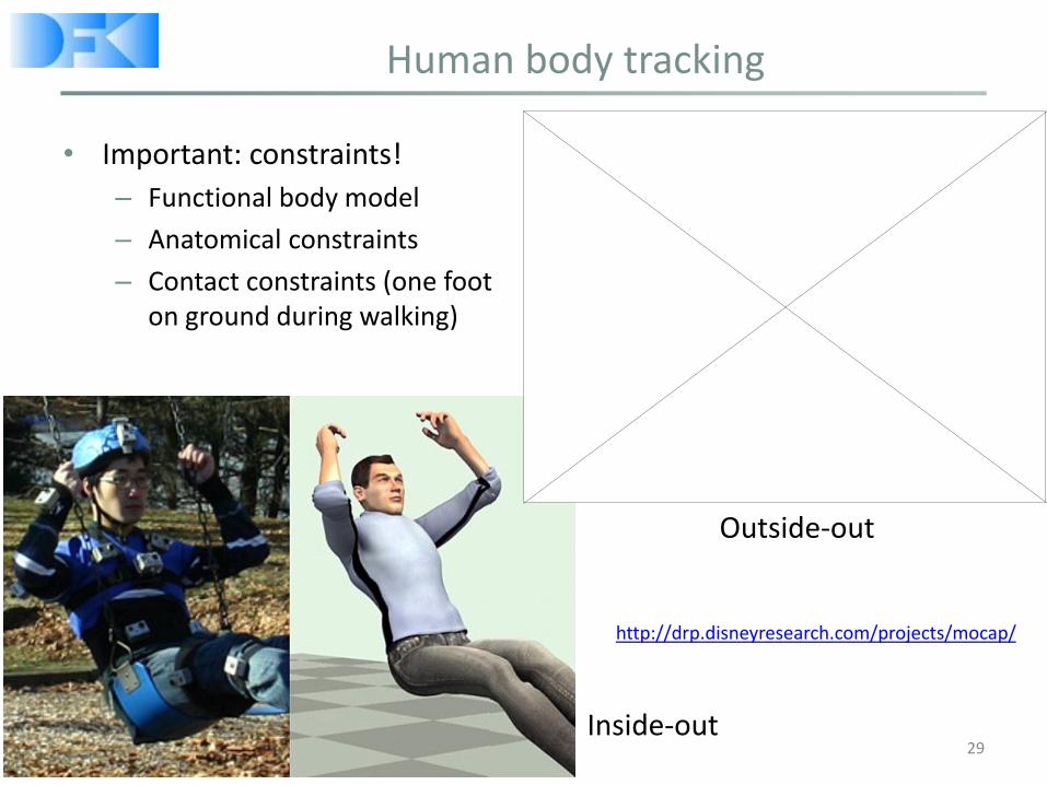
Human body tracking
• Important: constraints!
– Functional body model
– Anatomical constraints
– Contact constraints (one foot on ground during walking)
Inside-out
Outside-out
29
http://drp.disneyresearch.com/projects/mocap/

Head tracking inside a car
• Head-mounted camera and IMU
• How to overcome temporary feature occlusions?
Pure detection Visual-inertial tracking 30

Head tracking inside car mock-up
31

Objects Sensors
Models
Context
Modalities
Vision Data association
Object/people tracking
Object/
people tracking
Background modelling
32

Objects Sensors
Models
Context
Modalities
Vision Data association
Object/people tracking
Object/
people tracking
Background modelling Degrees of freedom
Appearance
Shape
Temporal dynamics
Target interactions
Environment constraints Noise characteristics
Detection/Prediction
Estimation
Likelihood
Data fusion (multimodal/-sensor/-target)
State update
33

+ + + ...
Multimodal data fusion
• Combine multiple information sources at different levels (texture, contours, edges)
• Improve adaptivity and robustness
34

Multi-sensor data fusion
• Combine information from several (complementary) sensors
• Improve robustness, adaptivity
35

x
x Missing detection
x
x
x
x x
False alarms
x Measurements
Predicted pose and covariances
Multi-target tracking: solve ambiguities
36

Predicted
shadow
Segmented
image
Error
image
Measurement likelihood
• How good is our prediction? – Pixel-level measurement
37

Measurement likelihood
• How good is our prediction? – Pixel-level measurement
– Feature-level measurement
Predicted
features
Matched
data
38
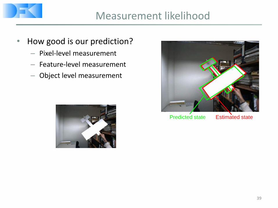
Measurement likelihood
• How good is our prediction? – Pixel-level measurement
– Feature-level measurement
– Object level measurement
Predicted state Estimated state
39

• Detection and loss detection: (re-)initialize the system
• Estimation: measurement processing and state update
• Models: all useful prior information about objects, sensors, and environment
t It Visual Processing
Measurement Prediction Output
Tracking Update
Loss It Object Detection
Initial estimate
Models
Shape Appearance Degrees of freedom
Dynamics Sensors Context
Detection
General tracking system (main components)
40

Summary
• Include model assumptions, e.g. motion models
• Overcome temporary tracking loss
• Predict future
• Fuse different sensor types and modalities
• Be robust
• Handle multiple targets
• Provide confidence values for estimates
• Handle multiple hypotheses
43

SA-1
How can we do all the things indicated before?
Probabilistic estimation framework: Bayesian filtering, recursive state estimation
Pre-requisites: probability theory, linear algebra

Introductory example
• Mobile robot localization in a known environment based on motion (odometry) and sensing (door detection)
• The robot knows a map of the environment (corridor with 3 indistinguishable doors)
• Wanted: position of the robot in the map
Source: Thrun et al., Probabilistic Robotics, 2005, MIT Press 45

Current position (state) is unknown.
Measurement z1: here is a door.
Momentary „belief“ of the robot
Measurement likelihood
Posterior belief after meas. update
46
Introductory example
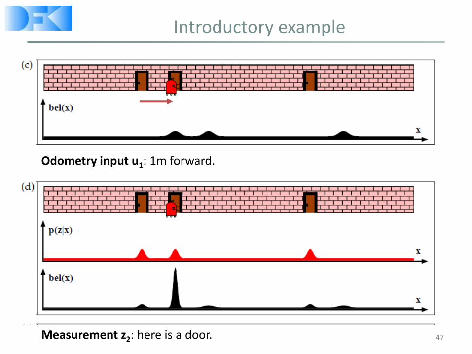
Odometry input u1: 1m forward.
Measurement z2: here is a door. 47
Introductory example

Odometry input u2: 1.5m forward.
• Bayes filter algorithm:
– Recursively estimate posterior belief or state distribution based on control data and sensor measurements
– Information represented as probability density function
– All entities are random variables
48
Introductory example

Recursive Bayesian filtering
• Key idea 1: Probability distributions represent our belief about the state of the dynamical system
• Key idea 2: Recursive cycle
1. Predict from motion model
2. Sensor measurement
3. Correct the prediction …repeat
predict
correct
measure
49

Recap: estimation methods
50
Non-probabilistic (e.g. LS) + quick convergence
+ efficient
- rely on momentary measurements
- stuck in local max/min
- modeling multiple objects
Probabilistic + consider history, entire probability densities, multi-modal
+ weaker requirements on accuracy of sensors/models
+ seamless integration of constraints, models
- slower (need to approximate)
- interpretation

Outline
• Basic concepts in probability
• Terminology, notation, probabilistic laws
• Bayes filters
51

SA-1
Basic concepts in probability

Discrete random variables
• 𝑋 denotes a random variable.
• 𝑋 can take on a countable number of values in {𝑥1, 𝑥2, … , 𝑥𝑛} according to probabilistic laws.
• 𝑝(𝑋 = 𝑥𝑖), or 𝑝(𝑥𝑖), is the probability that the random variable 𝑋 takes on value 𝑥𝑖.
• 𝑝(∙) is called probability mass function.
𝑝 𝑋 = 𝑥 = 1 𝑝(𝑋 = 𝑥) ≥ 0 𝑥
• Example:
– 𝑋 denotes the outcome of a coin flip
– For a fair coin: 𝑝 𝑋 = ℎ𝑒𝑎𝑑 = 𝑝 𝑋 = 𝑡𝑎𝑖𝑙 = 0.5
53

Continuous random variables
• 𝑋 takes on values in the continuum.
• 𝑝(𝑋 = 𝑥𝑖), or 𝑝(𝑥𝑖), is a probability density function (PDF).
𝑝 𝑥 𝑑𝑥 = 1
• Cumulative distribution funtion (CDF):
𝐹 𝑥 = 𝑝 𝑡 𝑑𝑡𝑥
−∞
• Probability of 𝑋 taking on a value in an interval:
𝑝 𝑎 < 𝑋 ≤ 𝑏 = 𝐹 𝑏 − 𝐹 𝑎 = 𝑝 𝑥 𝑑𝑥𝑏
𝑎
54
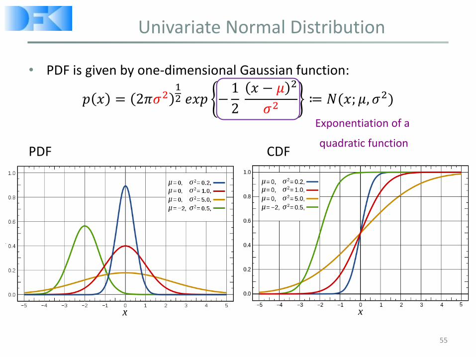
Univariate Normal Distribution
• PDF is given by one-dimensional Gaussian function:
𝑝 𝑥 = 2𝜋𝜎212 𝑒𝑥𝑝 −
1
2 𝑥 − 𝜇 2
𝜎2≔ 𝑁(𝑥; 𝜇, 𝜎2)
PDF CDF
55
Exponentiation of a
quadratic function

Multivariate Normal Distribution
• Normal distributions over vectors generalization of univariate normal distribution to higher dimensions
𝑝 𝑥 = 𝑑𝑒𝑡 2𝜋Σ12 𝑒𝑥𝑝 −
1
2 𝑥 − 𝜇 𝑇Σ−1(𝑥 − 𝜇)
≔ 𝑁(𝑥; 𝜇, Σ)
56
Covariance matrix (positive semidefinite,
symmetric matrix)
Mean vector
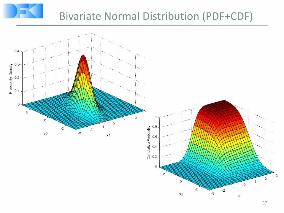
Bivariate Normal Distribution (PDF+CDF)
57

Statistics of probability distributions (1D)
• Expectation of a random variable: Discrete:
𝐸 𝑋 = 𝑥 𝑝(𝑥)
𝑥
Continuous:
𝐸 𝑋 = 𝑥 𝑝 𝑥 𝑑𝑥
• For arbitrary numerical values 𝑎 and 𝑏: 𝐸 𝑎𝑋 + 𝑏 = 𝑎𝐸 𝑋 + 𝑏
• Covariance of 𝑋 (expected squared deviation from mean): 𝐶𝑜𝑣 𝑋 = 𝐸 𝑋 − 𝐸 𝑋 2 = 𝐸 𝑋2 − 𝐸[𝑋]2
58

Joint and Conditional Probability
• Joint distribution of two random variables: 𝑝 𝑥, 𝑦 = 𝑝 𝑋 = 𝑥 𝑎𝑛𝑑 𝑌 = 𝑦
• Conditional distribution:
𝑝 𝑥 𝑦 = 𝑝 𝑋 = 𝑥 𝑌 = 𝑦 =𝑝 𝑥, 𝑦
𝑝(𝑦)
𝑝 𝑥, 𝑦 = 𝑝 𝑥 𝑦 𝑝(𝑦)
We know already that 𝑌’s value is 𝑦. What is the probability that 𝑋’s value is 𝑥 conditioned on that fact?
• If 𝑋 and 𝑌 are independent (carry no information about each other) then:
p 𝑥, 𝑦 = 𝑝 𝑥 𝑝 𝑦 𝑝 𝑥 𝑦 = 𝑝(𝑥)
59

Joint and Conditional Probability: example
• Ideal cube, dice toss: G={2, 4, 6}, A={4, 5, 6}
• 𝑝 𝐺 =?
• 𝑝 𝐴 =?
• 𝑝 𝐺, 𝐴 =?
• 𝑝 𝐺|𝐴 =?
60

Joint and Conditional Probability: example
• Ideal cube, dice toss: G={2, 4, 6}, A={4, 5, 6}
• 𝑝 𝐺 =1
2
• 𝑝 𝐴 =1
2
• 𝑝 𝐺, 𝐴 = 𝑝 4,6 =1
3
• 𝑝 𝐺|𝐴 =𝑝 𝐺,𝐴
𝑝(𝐴)= 2 𝑝 4,6 =
2
3
61

Theorem of Total Probability, Marginals
62
Discrete case
𝑝(𝑥)
𝑥
= 1
𝑝 𝑥 = 𝑝(𝑥, 𝑦)
𝑦
𝑝 𝑥 = 𝑝 𝑥 𝑦 𝑝(𝑦)
𝑦
Continuous case
𝑝 𝑥 𝑑𝑥∞
−∞
= 1
𝑝 𝑥 = 𝑝(𝑥, 𝑦)𝑑𝑦
𝑝 𝑥 = 𝑝 𝑥 𝑦 𝑝(𝑦) 𝑑𝑦

Bayes Theorem
• Relates a conditional to its „inverse“:
𝑝 𝑥, 𝑦 = 𝑝 𝑥 𝑦 𝑝 𝑦 = 𝑝 𝑦 𝑥 𝑝 𝑥
• Discrete case:
𝑝 𝑥 𝑦 =𝑝 𝑦 𝑥 𝑝 𝑥
𝑝(𝑦)=𝑝 𝑦 𝑥 𝑝 𝑥
𝑝 𝑦|𝑥′ 𝑝(𝑥′)𝑥′
• Continuous case:
𝑝 𝑥 𝑦 =𝑝 𝑦 𝑥 𝑝 𝑥
𝑝(𝑦)=𝑝 𝑦 𝑥 𝑝 𝑥
𝑝 𝑦|𝑥′ 𝑝(𝑥′) 𝑑𝑥′
63

Bayes Theorem: example
• 𝑌 = sum of two dice tosses (red and white die)
• 𝑋 = white die 𝑝 𝑋 = 4 𝑌 = 10 =?
• Bayes rule is useful, if 𝑝 𝑌 = 10|𝑋 = 4 is easier to compute than 𝑝 𝑋 = 4|𝑌 = 4
64

Bayes Theorem: example
• 𝑌 = sum of two dice tosses (red and white die)
• 𝑋 = white die 𝑝 𝑋 = 4 𝑌 = 10 =?
=𝑝 𝑌 = 10|𝑋 = 4 𝑝 𝑋 = 4
𝑝(𝑌 = 10)=
16∙16336
=1
3
• Bayes rule is useful, if 𝑝 𝑌 = 10|𝑋 = 4 is easier to compute than 𝑝 𝑋 = 4|𝑌 = 4
65
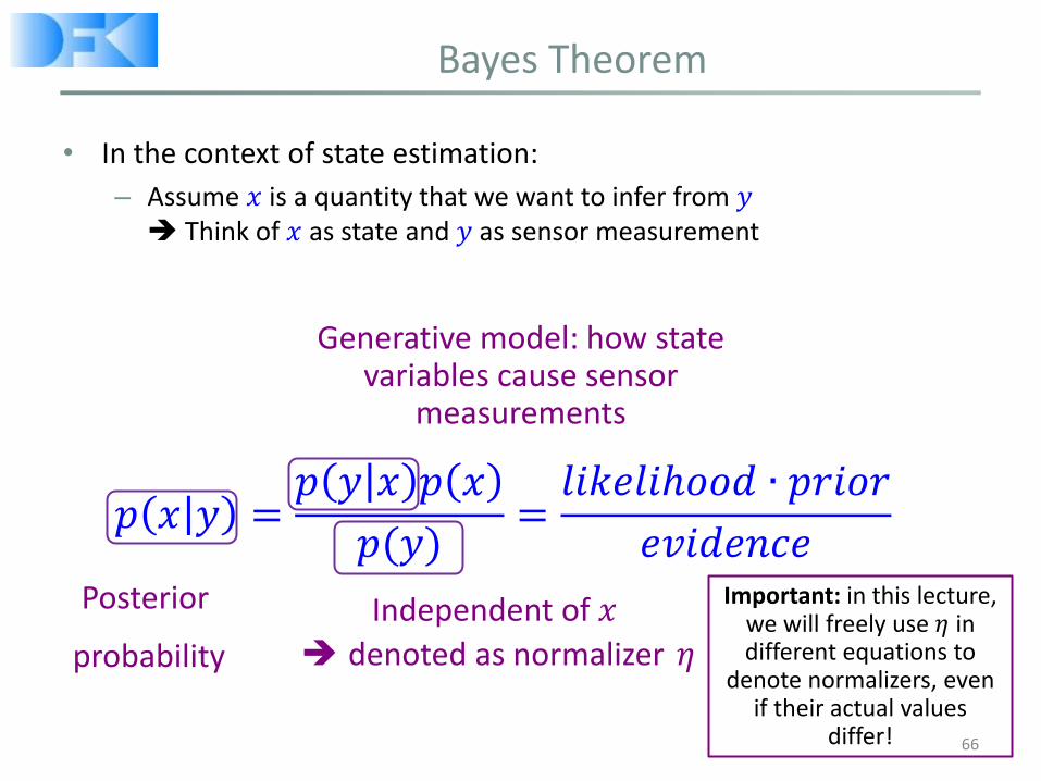
Bayes Theorem
• In the context of state estimation:
– Assume 𝑥 is a quantity that we want to infer from 𝑦 Think of 𝑥 as state and 𝑦 as sensor measurement
𝑝 𝑥 𝑦 =𝑝 𝑦 𝑥 𝑝 𝑥
𝑝(𝑦)=𝑙𝑖𝑘𝑒𝑙𝑖ℎ𝑜𝑜𝑑 ∙ 𝑝𝑟𝑖𝑜𝑟
𝑒𝑣𝑖𝑑𝑒𝑛𝑐𝑒
66
Posterior
probability
Generative model: how state variables cause sensor
measurements
Independent of 𝑥 denoted as normalizer 𝜂
Important: in this lecture, we will freely use 𝜂 in different equations to
denote normalizers, even if their actual values
differ!

Bayes Theorem
67

Conditional Independence
• All rules presented so far can be conditioned on an arbitrary random variable, e.g. Z
𝑝 𝑥 𝑦, 𝑧 =𝑝 𝑦 𝑥, 𝑧 𝑝 𝑥|𝑧
𝑝(𝑦|𝑧)
𝑝 𝑥, 𝑦 𝑧 = 𝑝 𝑥 𝑦, 𝑧 𝑝(𝑦|𝑧)
• Conditional Independence: 𝑥 and 𝑦 are independent, given that 𝑧 is known
𝑝 𝑥, 𝑦 𝑧 = 𝑝 𝑥 𝑧 𝑝 𝑦 𝑧 ⇔ 𝑝 𝑥 𝑧 = 𝑝 𝑥 𝑧, 𝑦 , 𝑝 𝑦 𝑧 = 𝑝(𝑦|𝑧, 𝑥)
does not necessarily imply absolute independence 68
𝑦 carries no information about 𝑥, if 𝑧 is known

Summary and outlook
Today:
• Recap: camera model, contour-based tracking
• Overview visual processing → Sensitizing: just a part of the story
• Introduction/motivation recursive state estimation
• Important probabilistic laws
Next lecture:
• State estimation: terminology, notation, probabilistic laws
• Bayes filter algorithm
69