Embed Size (px)
Citation preview
Expectations about the Federal Reserve’sBalance Sheet and the Term Structure
of Interest Rates∗
Jane Ihrig, Elizabeth Klee, Canlin Li,Min Wei, and Joe Kachovec
Board of Governors of the Federal Reserve System
This paper assesses the effects of the Federal Reserve’s assetpurchase programs on Treasury yields, and provides a frame-work to evaluate these effects both initially and over time asmarket expectations of the economy and the Federal Reserve’sbalance sheet evolve. Our framework suggests that the firstpurchase program had the largest initial impact on the ten-year Treasury yield, estimated to be about 34 basis points inearly 2009. Although the effect of the first program wanedconsiderably by the end of 2015, at that time all programscombined were depressing the ten-year yield by about 100basis points, reflecting expectations of economic conditions andFederal Reserve policy.
JEL Codes: G1, E4, C5.
1. Introduction
Through the financial crisis and subsequent recession, the FederalReserve introduced unconventional monetary policy actions in orderto “promote a stronger pace of economic recovery” and to helpensure that “inflation, over time, is at levels consistent with its man-date.”1 To this end, the Federal Reserve embarked on a number of
∗The opinions expressed in this paper are those of the authors and do notnecessarily reflect views of the Federal Reserve Board or the Federal Reserve Sys-tem. All errors are our own. Author contact: Ihrig: [email protected], +1 202-452-3372. Klee: [email protected], +1 202-721-4501. Li: [email protected],+1 202-452-2227. Wei: [email protected], +1 202-736-5619.
1Statement of the Federal Open Market Committee, November 3, 2010.
341
342 International Journal of Central Banking March 2018
asset programs to purchase, sell, or reinvest securities that dramat-ically changed the Federal Reserve’s securities holdings across alldimensions—size, composition, and maturity structure. Each assetprogram was implemented in part to put downward pressure onlonger-term interest rates, aimed to support a stronger recovery.
But how much did these asset programs affect longer-term inter-est rates? There is a growing body of work on this subject, which canbe divided into three broad categories. The first strand of researchdepends on event-study methodology to determine the effect of theasset programs on interest rates at the onset of the programs.2 Thesecond uses reduced-form regression analysis (either in a time seriesor using panel methods) to evaluate the effect of Federal Reservepurchases on interest rates over time.3 Finally, the third strand incor-porates changes in the net private supply of different assets into astructural model of the economy or the yield curve to evaluate theeffect of these programs on interest rates at any point in time.4 Thedynamic nature of this third type of model requires one to incorpo-rate information not only about the current level of System OpenMarket Account (SOMA) holdings but also about their expectedfuture path for an accurate estimate on interest rates. In this paper,we take the third approach.
More generally, the third approach incorporates features that arekey to understanding the overall impact of the asset purchase pro-grams. Most studies model the Federal Reserve’s asset purchases andsales as either occurring instantly or spread out evenly over a shortwindow. In reality, the purchases and sales were announced ahead oftime, followed a predetermined timetable where the pace sometimesvaried, and were commonly expected to be unwound at a future pointof time, resulting in changes not only to the contemporaneous levelof the Federal Reserve’s (Fed’s) balance sheet and private holdingsof Treasury securities and agency mortgage-backed securities (MBS)but also to expectations about their future dynamics. The dynamicpattern of the asset programs matters for the estimated impact on
2Refer to Gagnon et al. (2011), Krishnamurthy and Vissing-Jørgensen (2011),and Swanson (2011).
3Refer to D’Amico et al. (2012), Meaning and Zhu (2012), and D’Amico andKing (2013).
4Refer to Chung et al. (2011), Hamilton and Wu (2012), and Li and Wei(2013).
Vol. 14 No. 2 Expectations about the Fed’s Balance Sheet 343
interest rates. In addition, as the economy evolves, so do the expec-tations for the Fed’s securities holdings (including issues such as howto invest proceeds from maturing securities and when to stop thisreinvestment). Changing expectations have implications for how theFed’s actions affect yields on longer-term securities.
This paper develops a methodology that can be used to estimatethe effect of asset purchases on interest rates both at the initialoutset of a program and at any point in time thereafter. Impor-tantly, this approach is consistent with contemporaneous and futureinvestors’ expectations for the macroeconomy and Federal Reservepolicy, and therefore allows for a time-varying effect of a program oninterest rates. Specifically, this paper demonstrates how estimates ofinterest rate effects can be derived from longer-term market expec-tations of interest rates, macroeconomic conditions, and the FederalReserve’s balance sheet. To capture the projected time-series pat-terns of Federal Reserve portfolio holdings at any point in time, weuse the contemporaneous interest rate and macroeconomic projec-tions from the Blue Chip Economic Indicators release and Treas-ury issuance projections by the Congressional Budget Office (CBO).In addition, we assume a possible path for the unwinding of mone-tary policy accommodation consistent with the most recent FederalReserve communications regarding the removal of policy accommo-dation, or “normalization principles” at the date when the term pre-mium effect of a program is estimated. In particular, for those pur-chases announced before 2014, we use those outlined in the minutesof the June 2011 Federal Open Market Committee (FOMC) meeting;for those after, we use the update provided in the Policy Normal-ization Principles and Plans released in 2014. We project privateholdings of securities by recognizing that privately held securities aresimply the total stock of the securities outstanding minus the FederalReserve’s holdings.5 Taken together, these strategies ensure that ourestimates are consistent with market participants’ views of the evolu-tion of the economy and removal of unconventional monetary policy.
5In this context (and as defined by the U.S. Treasury), all marketable Treasurydebt that is not held by the Federal Reserve is considered to be “privately held,”even if that debt is held by foreign official accounts. In addition, currently thereis a small amount of marketable debt held by U.S. state and local governments;however, the level of these holdings relative to total marketable Treasury debt issmall.
344 International Journal of Central Banking March 2018
To construct our market-expectations-consistent projections ofFederal Reserve holdings, and hence private holdings, we lean on themethodology outlined in Carpenter et al. (2015). Their study consid-ers how the Federal Reserve’s balance sheet evolves with respect toboth the Federal Reserve’s projected unwinding of unconventionalmonetary policy accommodation and the “natural” evolution of thebalance sheet that accounts for increases in currency and growth inFederal Reserve bank capital.6 The dollar amount of each asset pur-chase program and the maturity structure of the purchases and salesof securities also affect the expected evolution of the balance sheet,which is critical for determining the term premium effect (TPE).These characteristics are embedded in the estimates presented belowand provide a view of how market participants perceived each assetprogram when it was implemented, as well as what is expected as oftoday.
When assessing the interest rate effects of the Federal Reserve’sasset programs, we focus on the “duration” channel through whichFederal Reserve purchases reduce the quantity and the averagematurity of long-term safe assets held by private investors and lowerthe term premiums on these assets.7 In particular, we adopt themodel of Li and Wei (2013), which was motivated by empiricalevidence that excess bond returns appear to be predictable by theamount and the average maturity of Treasury securities outstanding,as well as the theoretical work of Vayanos and Vila (2009), whichshows how differences in maturity preferences of Treasury investorscan generate supply effects in the government bond market.8 In theLi and Wei (2013) model, Treasury yields are driven by both yieldfactors and Treasury and agency MBS supply factors. They use themodel to evaluate the magnitude of supply effects on term premi-ums, and find that a 1 percentage point decline in the ratio of private
6One focus of that work was on the nature of the interest rate shocks thatcould lead to the Federal Reserve’s remittances to Treasury ceasing for a period.This paper does not focus on that issue to the same extent; other papers, includ-ing Greenlaw et al. (2013) and Christensen, Lopez, and Rudebusch (2015), pro-vide alternative views on the interest rate risk inherent in the Federal Reserve’sportfolio.
7Other potential channels are discussed in the literature review section below.8Greenwood and Vayanos (2014) illustrate that there are supply effects from
overall Treasury debt outstanding on the term structure of interest rates.
Vol. 14 No. 2 Expectations about the Fed’s Balance Sheet 345
holdings of Treasury ten-year equivalents to GDP ratio or the MBSpar-to-GDP ratio would reduce the ten-year Treasury yield by about10 basis points, while a one-year shortening of the average effectiveduration of private MBS holdings would lower the ten-year Treasuryyield by about 7 basis points.
By combining estimates of market expectations for the FederalReserve’s portfolio, interest rates, and macroeconomic conditionsconstructed above with this term structure model, we are able totake a comprehensive view of both the term structure of interestrates and the size and composition of the Federal Reserve balancesheet. As a result, the estimated interest rate effects of the FederalReserve’s asset programs are consistent with market expectationsabout how private holdings of securities will evolve at any point intime with all asset programs in place at that date. This approachallows us to estimate the TPE at the onset of an asset program,to track the expected “decay” of the program, and to evaluate theTPE and its decay at any other point in time using updated marketexpectations.
The main contributions of this paper are twofold. First, we pro-vide a time-varying, market-expectations-consistent estimate of theTPE as the economy evolves and expected FOMC policies adjust,while most other studies focus on the TPE at the onset of the assetprograms. Second, we can estimate the expected decay of the TPE.The evolution of the TPE illustrates how past unconventional mon-etary policy will fade over the next several years, exerting down-ward pressure on longer-term interest rates even after the FOMChas raised the federal funds rate above zero.
Relative to other studies, this approach is more comprehen-sive and, therefore, provides a more complete estimate of the TPE.For example, Chung et al. (2012) use the par value of the FederalReserve’s Treasury and agency MBS holdings to estimate their TPE,and are therefore not equipped to provide TPE estimates for someof the asset programs that hold the level of securities constant butchange the composition of holdings. Li and Wei (2013) use a rule-of-thumb proxy for the evolution of private holdings of securities and,therefore, focus only on the contemporaneous impact of the asset pro-grams. Here, we align our projections of private holdings with marketparticipants’ views about the expected path of Treasury issuance andfuture Federal Reserve holdings of securities and, as a result, have
346 International Journal of Central Banking March 2018
a contemporaneous estimate of the TPE of each asset program atimplementation that is consistent with market expectations, havea projection of the expected TPE over time (TPE path) based onthose expectations, and have the ability to reevaluate the TPE pathwith updated expectations at any future point in time.9 Moreover,while this methodology requires constructing views on how the cen-tral bank’s balance sheet evolves with and without a particular assetpurchase program, and therefore is more complicated than an event-study approach, it is at the same time flexible and complete enoughto produce estimates of monetary policy accommodation over timethat are consistent with preferred-habitat models of asset purchases.
We evaluate the term premium effect of each of the sevenasset programs conducted by the Federal Reserve from 2008 to2014—the outright purchase programs announced on November2008 and expanded in March 2009 (LSAP1); the reinvestment pro-gram announced in August 2010; the outright purchase programannounced in November 2010 (LSAP2); the maturity extension pro-gram (MEP) announced in September 2011; the change to the rein-vestment program announced in September 2011; the continuationof the MEP announced in June 2012; and the open-ended purchaseprogram that commenced in the fall of 2012. We investigate how theten-year Treasury term premium reacted at the time of each pro-gram’s inception based on market expectations that were in place atthe time, and we also examine how each program continues to affectinterest rates today, using current expectations. Our estimates sug-gest that at inception, the first LSAP program resulted in the largestapparent reduction in the ten-year Treasury term premium of about34 basis points in the second quarter of 2009, the maturity extensionprogram taken as a whole held down the term premium by about 28basis points, and the open-ended purchase program depressed theterm premium by 31 basis points.
These estimates of the term premium effect are based on mar-ket participants’ views of the evolution of the economy at the timethat each asset program was implemented. However, through time,expectations changed. For example, the June 2009 Blue Chip Fore-cast expected that the federal funds rate would rise above 25 basis
9Engen, Laubach, and Reifschneider (2015) use our estimate in their paper.
Vol. 14 No. 2 Expectations about the Fed’s Balance Sheet 347
points by June 2010 and that annual GDP growth would return to3.1 percent by 2011, while in reality the federal funds rate stayed atthe effective lower bound until end-2015 and annual GDP growth hasyet to reach 3 percent. Also, the FOMC originally viewed MBS salesas part of the exit strategy but in 2012 announced that only residualsales could possibly be conducted at some point in the future. Impor-tantly, our model allows us to update the TPEs of each program forcurrent and evolving market expectations.
All of these asset purchases were completed as of the fourthquarter of 2014, and only the reinvestment programs were ongo-ing through 2015. Towards the end of 2015, after all purchases werecompleted and the FOMC was preparing to raise interest rates forthe first time in many years, the TPEs of all programs combined isestimated to be about 100 basis points. We attribute about 5 basispoints to the first large-scale asset purchase program, a negligibleamount to the second; about 20 basis points each to the matu-rity extension program and its continuation; a little over 20 basispoints to the third; and the remainder to the reinvestment programs.In addition, we present a measure of uncertainty around the termpremium effect by calculating error bands around our point esti-mate. Overall, the results suggest about a wide 90 basis point confi-dence interval around our term premium effect. In the first quarterof 2015, the standard error on our TPE estimate is 27 basis points,representing roughly one-quarter of our estimate.
2. Background
This section reviews the purchase programs during the financial cri-sis that shaped the Federal Reserve’s balance sheet and the theorybehind our model. We discuss each in turn.
2.1 The Federal Reserve’s Balance Sheetand the SOMA Portfolio
In order to have a comprehensive estimate of how the FederalReserve’s asset programs affected private-sector holdings of secu-rities, one must consider how the SOMA evolves over time bothwith and without these programs. To help understand this point,
348 International Journal of Central Banking March 2018
we briefly review a few key line items of the balance sheet; a moredetailed discussion is in Carpenter et al. (2015).
For most of the postwar period, the largest asset on the FederalReserve’s balance sheet was the SOMA, and the largest liability wasFederal Reserve notes (FR Notes), or paper currency, in circulationoutside of reserve banks.10 Growth of the Federal Reserve’s balancesheet reflected growth in currency outstanding, as well as increasesin Reserve Bank capital. As currency and capital grew, the FederalReserve purchased Treasury securities in the open market to keepassets on the Federal Reserve’s balance sheet equal to liabilities pluscapital.
In addition to steady growth, the composition of the SOMA port-folio was fairly constant as well. Over time, the Federal Reserve helda few types of securities in the SOMA portfolio, and from 2004through the financial crisis, the portfolio held only Treasury secu-rities. The weighted-average maturity of the portfolio ranged fromthree to four years. In addition, as expressed in ten-year equivalents,or duration equivalents of the on-the-run ten-year note, the SOMAportfolio grew at a pace similar to the par growth rate of the portfo-lio, although it fluctuated some as the duration of the ten-year notechanged.11
The Federal Reserve’s balance sheet changed markedly with thestart of the financial crisis, and in ways that both indirectly anddirectly affected the evolution of the Federal Reserve’s securitiesholdings. The first actions were engaging in reserve-adding repur-chase agreements and lowering the rate on discount window loans inAugust 2007. Subsequently, credit and lending facilities were intro-duced to aid with liquidity strains. These actions included the TermAuction Facility (TAF), which granted banks term loans of centralbank funds, in the fall of that year. All of these actions expandedthe asset side of the balance sheet. As a result, the Open MarketDesk allowed some Treasury bills to mature and sold other securi-ties in order to sterilize these reserve-adding actions. As a result of
10The remainder of the assets on the balance sheet—for example, borrow-ings from the discount window, other assets, and foreign exchange assets—wasrelatively small when compared with the SOMA portfolio.
11A Treasury security expressed in ten-year equivalents is the par value ofsecurity times the duration of security divided by the duration of the on-the-runten-year Treasury note.
Vol. 14 No. 2 Expectations about the Fed’s Balance Sheet 349
the sterilization, Treasury bill holdings in the SOMA dropped to alittle less than $20 billion in June 2008.
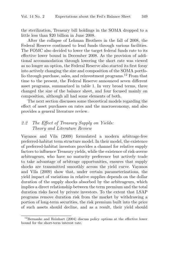
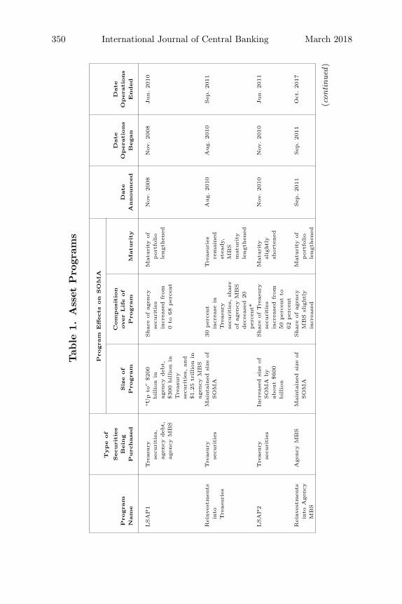
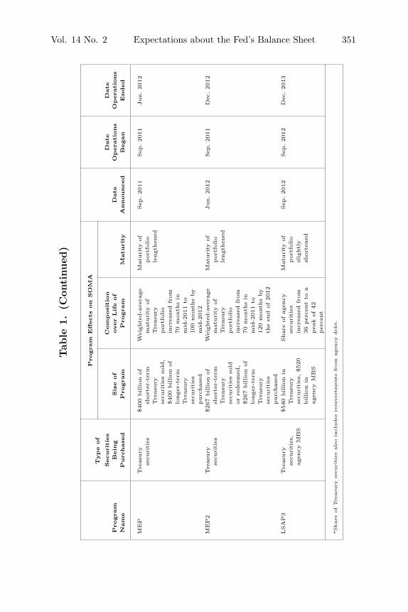
After the collapse of Lehman Brothers in the fall of 2008, theFederal Reserve continued to lend funds through various facilities.The FOMC also decided to lower the target federal funds rate to itseffective lower bound in December 2008. As the provision of addi-tional accommodation through lowering the short rate was viewedas no longer an option, the Federal Reserve also started its first forayinto actively changing the size and composition of the SOMA portfo-lio through purchase, sales, and reinvestment programs.12 From thattime to the present, the Federal Reserve announced seven differentasset programs, summarized in table 1. In very broad terms, threechanged the size of the balance sheet, and four focused mainly oncomposition, although all had some elements of both.
The next section discusses some theoretical models regarding theeffect of asset purchases on rates and the macroeconomy, and alsoprovides a general literature review.
2.2 The Effect of Treasury Supply on Yields:Theory and Literature Review
Vayanos and Vila (2009) formulated a modern arbitrage-freepreferred-habitat term structure model. In their model, the existenceof preferred-habitat investors provides a channel for relative supplyfactors to influence Treasury yields, while the existence of risk-aversearbitrageurs, who have no maturity preference but actively tradeto take advantage of arbitrage opportunities, ensures that supplyshocks are transmitted smoothly across the yield curve. Vayanosand Vila (2009) show that, under certain parameterizations, theyield impact of variations in relative supplies depends on the dollarduration of the supply shocks absorbed by the arbitrageurs, whichimplies a direct relationship between the term premium and the totalduration risks faced by private investors. To the extent that LSAPprograms remove duration risk from the market by withdrawing aportion of long-term securities, the risk premium built into the priceof such assets should decline, and as a result, their yield should
12Bernanke and Reinhart (2004) discuss policy options at the effective lowerbound for the short-term interest rate.
350 International Journal of Central Banking March 2018
Tab
le1.
Ass
etP
rogr
ams
Type
of
Pro
gra
mEffects
on
SO
MA
Securi
ties
Com
posi
tion
Date
Date
Pro
gra
mB
ein
gSiz
eof
over
Life
of
Date
Opera
tions
Opera
tions
Nam
eP
urc
hase
dP
rogra
mP
rogra
mM
atu
rity
Announced
Began
Ended
LSA
P1
Tre
asu
ryse
curi
ties
,agen
cydeb
t,agen
cyM
BS
“U
pto
”$200
billion
inagen
cydeb
t,$300
billion
inTre
asu
ryse
curi
ties
,and
$1.2
5tr
illion
inagen
cyM
BS
Share
ofagen
cyse
curi
ties
incr
ease
dfr
om
0to
68
per
cent
Matu
rity
of
port
folio
length
ened
Nov
.2008
Nov
.2008
Jun.2010
Rei
nves
tmen
tsin
toTre
asu
ries
Tre
asu
ryse
curi
ties
Main
tain
edsi
zeof
SO
MA
30
per
cent
incr
ease
inTre
asu
ryse
curi
ties
,sh
are
ofagen
cyM
BS
dec
rease
d20
per
cent*
Tre
asu
ries
rem
ain
edst
eady,
MB
Sm
atu
rity
length
ened
Aug.2010
Aug.2010
Sep
.2011
LSA
P2
Tre
asu
ryse
curi
ties
Incr
ease
dsi
zeof
SO
MA
by
about
$600
billion
Share
ofTre
asu
ryse
curi
ties
incr
ease
dfr
om
50
per
cent
to62
per
cent
Matu
rity
slig
htl
ysh
ort
ened
Nov
.2010
Nov
.2010
Jun.2011
Rei
nves
tmen
tsin
toA
gen
cyM
BS
Agen
cyM
BS
Main
tain
edsi
zeof
SO
MA
Share
ofagen
cyM
BS
slig
htl
yin
crea
sed
Matu
rity
of
port
folio
length
ened
Sep
.2011
Sep
.2011
Oct
.2017
(con
tinu
ed)
Vol. 14 No. 2 Expectations about the Fed’s Balance Sheet 351
Tab
le1.
(Con
tinued
)
Type
of
Pro
gra
mEffects
on
SO
MA
Securi
ties
Com
posi
tion
Date
Date
Pro
gra
mB
ein
gSiz
eof
over
Life
of
Date
Opera
tions
Opera
tions
Nam
eP
urc
hase
dP
rogra
mP
rogra
mM
atu
rity
Announced
Began
Ended
MEP
Tre
asu
ryse
curi
ties
$400
billion
of
short
er-t
erm
Tre
asu
ryse
curi
ties
sold
,$400
billion
of
longer
-ter
mTre
asu
ryse
curi
ties
purc
hase
d
Wei
ghte
d-a
ver
age
matu
rity
of
Tre
asu
ryport
folio
incr
ease
dfr
om
70
month
sin
mid
-2011
to100
month
sby
mid
-2012
Matu
rity
of
port
folio
length
ened
Sep
.2011
Sep
.2011
Jun.2012
MEP2
Tre
asu
ryse
curi
ties
$267
billion
of
short
er-t
erm
Tre
asu
ryse
curi
ties
sold
or
redee
med
,$267
billion
of
longer
-ter
mTre
asu
ryse
curi
ties
purc
hase
d
Wei
ghte
d-a
ver
age
matu
rity
of
Tre
asu
ryport
folio
incr
ease
dfr
om
70
month
sin
mid
-2011
to120
month
sby
the
end
of2012
Matu
rity
of
port
folio
length
ened
Jun.2012
Sep
.2011
Dec
.2012
LSA
P3
Tre
asu
ryse
curi
ties
,agen
cyM
BS
$540
billion
inTre
asu
ryse
curi
ties
,$520
billion
inagen
cyM
BS
Share
ofagen
cyse
curi
ties
incr
ease
dfr
om
36
per
cent
toa
pea
kof42
per
cent
Matu
rity
of
port
folio
slig
htl
ysh
ort
ened
Sep
.2012
Sep
.2012
Dec
.2013
*Share
ofTre
asu
ryse
curi
ties
als
oin
clu
des
rein
vest
ments
from
agency
debt.
352 International Journal of Central Banking March 2018
decline. The removal of duration risk should generate reactions ofyields across much of the maturity spectrum—not just on the yieldsof purchased securities but on those of adjacent maturities as well.
Motivated by this theory, Li and Wei (2013) propose and estimatean arbitrage-free term structure model with supply factors includingthe private holdings of Treasury and agency MBS securities. Theyshow that these supply factors have important explanatory poweron the term premium beyond that embedded in traditional yield-curve factors. They also derive a formula that links the term pre-mium to current and expected future shocks to these supply factors.As a result, their model can be used to evaluate an asset purchaseprogram’s term premium effect based on the program’s projectedimpacts over time on these supply factors.
Of course, there are other plausible modeling approaches thatdiffer from the one we have chosen here. While the Li-Wei paperemphasizes the duration risk channel through which the FederalReserve’s asset programs work on reducing longer term rates, otherpapers have emphasized additional channels. For example, Krishna-murthy and Vissing-Jørgensen (2011) offer evidence that Treasurysupplies could also affect interest rates through what they call “thesafety premium channel.” Another example is D’Amico and King(2013); their work emphasizes the “scarcity channel,” or the avail-able supply of nearby maturities. D’Amico et al. (2012) also focuson the scarcity channel in their analysis; they couple this channelwith the duration channel to arrive at their final estimates of theterm premium effects of the programs.
Finally, other approaches emphasize the “signaling” channel,whereby announcements of purchases by the central bank signalthat accommodative federal funds rate policy would remain in placefor some time. Researchers, including Bauer and Rudebusch (2014),illustrate the importance of this channel. Our modeling approachspecifically abstracts from this channel, as we focus on the term pre-mium effect of asset purchases. However, as will be explained furtherbelow, our modeling approach does indirectly incorporate marketexpectations for the federal funds rate. In particular, investors typi-cally expect a link between the timing of any federal funds rate tight-ening and the timing when the Federal Reserve will allow securitiesto mature off its balance sheet. If any LSAP program announce-ment simultaneously lowered market expectations for the path of
Vol. 14 No. 2 Expectations about the Fed’s Balance Sheet 353
the federal funds rate, our modeling approach would suggest thatthe balance sheet would remain larger for longer and, as such, theterm premium effect would be magnified. All told, then, while ourterm premium effect estimate does not reflect a signaling channel,it does incorporate at least some of the effect on rates attributableto expectations for a lower federal funds rate path.
There are also alternative choices for modeling private holdingsof securities. One example is in Chung et al. (2011), which usesthe differences in the SOMA-to-GDP ratio from a long-run aver-age as a proxy for changes in private holdings of securities dueto LSAPs, and as such, uses balance sheet projections to evaluateLSAPs. That said, their approach has a few shortcomings. Specif-ically, they approximate the balance sheet contours by looking atthe current par value of SOMA holdings and assume that SOMAholdings in excess of one year remaining maturity trend towards along-run level of 5 percent of nominal GDP. This approximation isreasonable for a “rough estimate” of the TPE associated with theLSAP programs, but the results depend critically on the assumptionfor the steady-state SOMA-to-GDP ratio, which changes over time.In addition, while their methodology likely gives similar results tothose presented here for the LSAP1 and LSAP2 purchase programs,it cannot evaluate the effect of the MEP or any asset purchase pro-grams that change the duration of SOMA but not the nominal valueof the portfolio. That methodology also fails to take into account anyendogenous, cyclical variations in the SOMA-to-GDP ratio.
3. The Model
This section reviews the two aspects of our modeling efforts: theterm structure model with supply factors, and the construction ofthe path of private-sector holdings of securities. We discuss each inturn.
3.1 Modeling the Term Premium Effect
Li and Wei (2013) assume that yields are driven by five state vari-ables, denoted by ft, that include two yield-curve factors (level andslope), one Treasury supply factor (total private holdings of Treasurysecurities in terms of ten-year equivalents and as a ratio of nominal
354 International Journal of Central Banking March 2018
GDP), and two agency MBS supply factors (the par amount of totalprivate holdings of MBS as a ratio of nominal GDP and averageMBS duration), numbered 1 through 5.
The inclusion of these supply factors is motivated by thepreferred-habitat term structure model as in Vayanos and Vila(2009). That model has two types of private participants in theTreasury market: preferred-habitat investors, who hold only a par-ticular maturity segment of the Treasury yield curve and are riskneutral, and risk-averse arbitrageurs, who trade to take advantageof arbitrage opportunities and have no maturity preference. Vayanosand Vila (2009) show that in such a model, bond holdings of the arbi-tragers can affect the equilibrium bond risk premiums. The supplyfactors included in Li and Wei (2013) as well as in this paper canbe justified by the additional assumption that the preferred-habitatinvestors consist of the U.S. Treasury and the Federal Reserve, whilethe arbitrageurs correspond to the entire private sector.13
The state variables are assumed to follow a first-order vectorautoregressive process:
ft+1 = c + ρft + Σεt+1, (1)
with the following restrictions:
ρ =
⎡⎢⎢⎢⎢⎣
ρ11ρ2100
ρ51
ρ12ρ22000
00
ρ3300
000ρ440
0000
ρ55
⎤⎥⎥⎥⎥⎦,
∑=
⎡⎢⎢⎢⎢⎣
σ11000
σ51
0σ22000
00
σ3300
000σ440
0000
σ55
⎤⎥⎥⎥⎥⎦,
where the non-zero ρ51 captures the feedback effect from the level ofinterest rates to average MBS duration. The restriction that Treas-ury and MBS holdings factors do not load on past yield factors(ρij = 0, 3 ≤ i ≤ 4, 1 ≤ j ≤ 2) reflects the empirical evidence thatthe net issuance of both Treasury securities and of agency MBS doesnot react strongly to interest rates in the short run.14
13The same assumption is used by Hamilton and Wu (2012).14The Treasury’s stated debt-management policy is that it does not “time the
market”—or seek to take advantage of low interest rates—when it issues secu-rities. Instead, the Treasury strives to lower its borrowing costs over time by
Vol. 14 No. 2 Expectations about the Fed’s Balance Sheet 355
The one-period nominal short rate is assumed to be linear in thefactors
y1t = a1 + b′1ft, (2)
with the restriction that it only loads on the yield factors:
b1 =[b11 b12 0 0 0
]′.
Under this restriction, shocks to supply factors do not affectinterest rate expectations but can affect bond yields through theterm premium channel only. This assumption captures the fact thatthe supply of Treasury and MBS securities is not an importantconsideration when the Fed determines the short-term interest rate.
The stochastic discount factor is conditionally log-normal,
log Mt = −y1t − 12λ′
tλt − λ′tεt+1, (3)
with the market prices of risk also assumed to be affine in the factors:
λt = λ0 + λ1ft. (4)
We impose the restriction that the supply factors do not carrytheir own risk premiums but can affect term premiums by changingthe risk premiums on the yield factors. As a result, we can restrictthe last three rows of b1 to be zero. This assumption reflects ourprior that Treasury and MBS supplies are unlikely to be a source ofundiversifiable risk that should be priced on its own. Imposing theserestrictions on the short rate and risk premiums also helps reducethe number of parameters that needs to estimated and avoid theoverfitting problem.
Under all these assumptions, it is relatively easy to solve for theprice Pn
t of an n-period zero-coupon bond at time t by recursivelysolving the relation
Pnt = Et(MtP
n−1t+1 ), (5)
relying on a “regular and predictable” preannounced schedule of auctions. Whilethe gross issuance of MBS responds strongly to the level of rates in a refinanceboom sparked by declining interest rates, the net supply of MBS stays aboutunchanged as old mortgages and MBS are replaced with new ones.
356 International Journal of Central Banking March 2018
with the terminal condition P 0t = 1. The resulting bond prices are
exponential linear functions of the state vector:
Pnt = exp(An + Bnft), (6)
with
An+1 = An + B′n (c − Σλ0) +
12B′
nΣΣ′Bn − a1 and (7)
Bn+1 = (ρ − Σλ1)′Bn − b1, (8)
and the initial conditions A1 = −a1 and B1 = −b1. Bond yields arethen given by
ynt = an + bnft, (9)
where an = −An
n and bn = −Bn
nLi and Wei (2013) estimate this model using monthly data on
Treasury yields, private holdings of Treasury and agency MBS, andaverage MBS durations from March 1994 to July 2007, which pro-vides model-implied loadings of yields on the factors bn. Given theseloading estimates, the impact of an asset purchase program canbe easily estimated by first calculating the expected shocks to thefirst two supply factors—private holdings of Treasury securities andagency MBS—associated with each program, and then multiplyingit by the term premium loadings; the MBS average duration factor isendogenously determined inside the model but not directly affectedby the asset purchase programs.
This simple approach, however, treats the purchases as one-period shocks to these two supply variables with the implicit assump-tion that following the shocks, those supply variables will resumetheir evolution over time according to their historical dynamics. Incontrast, the asset purchase programs are usually implemented overa period of time, resulting in predictable or expected changes to boththe levels and the dynamics of the Treasury and MBS private hold-ings factors during and after the purchases. Therefore, the LSAPprograms in practice represent a series of expected shocks to supplyfactors and are modeled as such in and Li and Wei (2013). In par-ticular, they show that the cumulative effect of a series of expected
Vol. 14 No. 2 Expectations about the Fed’s Balance Sheet 357
supply shocks on yields over the life of the bond can be measuredby the following formula:
ynt − yn
t = bsnus
t +T−t∑i=1
n − i
nbsn−i(u
st+i − ρssus
t+i−1)
≈ bsnus
t +T−t∑i=1
n − i
nbsn−i(u
st+iu
st+i−1), (10)
where ynt − yn
t is the difference in the bond yield with and withoutthe expected supply shock to the Treasury and MBS private hold-ings, bs
n denotes the loadings of yields on these two supply factors,us
t = [uTsyt , uMBS
t ] denotes the exogenous shocks to these two sup-ply factors at time t, and ρss denotes the autoregressive matrix ofthe supply variables. For Treasury securities, uTsy
t is the differencebetween Federal Reserve holdings of Treasury securities (in termsof ten-year equivalents and as a percentage of nominal GDP) in ascenario without the asset purchase program and a scenario withthe program, while for agency MBS, uMBS
t is the difference betweenFederal Reserve agency MBS holdings (in par amount and as a per-centage of nominal GDP) in a scenario without the asset purchaseprogram and a scenario with the program.15
As noted in equation (10), the term premium effect dependsnot only on the current supply shock us
t but also on the expectedfuture path of us. In Li and Wei (2013), as an illustrative usage ofthe model, the us path is constructed simply as three phases foreach asset program: a smooth increase during the program imple-mentation phase, staying at this level for two years (the holdingphase), and then a smooth decline over time that dissipates overfive years (the unwinding phase). Here, we model the evolution ofthe us by making it consistent with market participants’ views on theevolution of Treasury issuance and Federal Reserve holdings, withthe latter accounting for the expected unwind of monetary policyaccommodation provided by the balance sheet.16
15Keeping the total amount outstanding constant, the changes in private hold-ings are equal in magnitude but opposite in sign to changes in Federal Reserveholdings.
16More details of the construction of us are discussed below.
358 International Journal of Central Banking March 2018
3.2 Modeling the Federal Reserve’s Balance Sheet
As discussed above, the term premium effect relies on the projectedpath of shocks to private-sector holdings of securities. We constructthis path by projecting the evolution of total Treasury issuance andFederal Reserve holdings of securities.17 Both are critical to evaluateaccurately the evolution of supply shocks discussed above.
The remainder of this section briefly reviews the constructionof the Federal Reserve’s holdings of securities; more specifics of themethodology can be found in Carpenter et al. (2015) and in theappendix.
To estimate the TPE for a given asset program upon implemen-tation, we project how the SOMA portfolio evolved in two scenarios:(i) a projection of SOMA holdings immediately after the onset of theprogram (using expectations by market participants at that point intime) that includes the asset purchases to be studied; and (ii) a pro-jection of SOMA holdings immediately prior to the announcementand implementation of the asset program under consideration butwith no additional asset purchases (the counterfactual). An impor-tant counterfactual that we construct reflects the possible evolutionof the balance sheet without any asset purchases at all. This coun-terfactual is a scenario where the economy evolved as market par-ticipants expected in October 2008; that is, without asset purchasesand without a severe recession. This translated to a somewhat stan-dard Federal Reserve balance sheet, with small asset holdings thatprimarily support currency in circulation.
For each scenario, we project the evolution of the balance sheetreflecting in part the maturity profile of the securities held in theportfolio. This evolution is based on the announced maturity struc-ture of the asset purchase programs, the projection of the compo-sition of total Treasury debt outstanding, and the growth in thesize of the balance sheet attributable to factors other than the assetpurchases.
Another key part of modeling the effect of asset purchase pro-grams is the assumption surrounding the removal of balance sheet
17We assume that total securities outstanding are exogenous to the FederalReserve’s asset programs. This is consistent with the Treasury not altering theirfunding patterns after the initiation of the various Federal Reserve’s asset pur-chase programs.
Vol. 14 No. 2 Expectations about the Fed’s Balance Sheet 359
policy accommodation. For programs announced before 2013, webase our projections on the general principles for the exit strategythat the FOMC outlined in the minutes of the June 2011 FOMCmeeting. At that time, the Committee stated that it intended totake steps in the following order:
(i) Cease reinvesting some or all payments of principal on thesecurities holdings in the SOMA.
(ii) Modify forward guidance on the path of the federal funds rateand initiate temporary reserve-draining operations aimed atsupporting the implementation of increase in the federal fundsrate when appropriate.
(iii) Raise the target federal funds rate.(iv) Sell agency securities over a period of three to five years.(v) Once sales begin, normalize the size of the balance sheet over
two to three years.18
However, the Policy Normalization Principles and Plans releasedin September 2014 suggest that (i) ceasing reinvestment will notoccur until after liftoff and (ii) MBS sales would not be a promi-nent part of the early stages of policy normalization. As such, werely on these revised Principles and Plans for the open-ended assetpurchase program and subsequent reinvestments. More broadly, theassumptions regarding the removal of policy accommodation affectthe contour of the balance sheet and, therefore, the amount ofaccommodation provided: as the balance sheet with the asset pur-chases comes to resemble that without them, policy accommodationwanes.
To complete the normalization strategy, we make a few additionalassumptions. We tie changes in the SOMA portfolio to the date thefederal funds rate rises from its effective lower bound. For programsimplemented prior to the open-ended purchases, we assume that thereinvestment of securities ends six months before this date and weassume that sales of agency securities begin six months after thefederal funds rate begins to rise. For the open-ended purchase pro-gram implemented over 2012 to 2014 and for the estimate of the
18Minutes of the Federal Open Market Committee, June 21–22, 2011, availableat http://www.federalreserve.gov/monetarypolicy/files/fomcminutes20110622.pdf.
360 International Journal of Central Banking March 2018
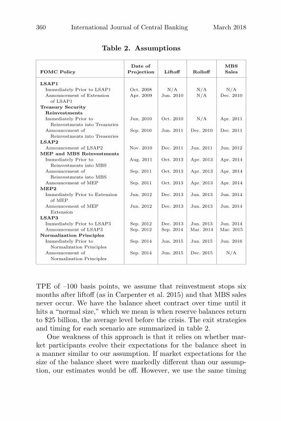
Table 2. Assumptions
Date of MBSFOMC Policy Projection Liftoff Rolloff Sales
LSAP1Immediately Prior to LSAP1 Oct. 2008 N/A N/A N/AAnnouncement of Extension
of LSAP1Apr. 2009 Jun. 2010 N/A Dec. 2010
Treasury SecurityReinvestmentsImmediately Prior to
Reinvestments into TreasuriesJun. 2010 Oct. 2010 N/A Apr. 2011
Announcement ofReinvestments into Treasuries
Sep. 2010 Jun. 2011 Dec. 2010 Dec. 2011
LSAP2Announcement of LSAP2 Nov. 2010 Dec. 2011 Jun. 2011 Jun. 2012
MEP and MBS ReinvestmentsImmediately Prior to
Reinvestments into MBSAug. 2011 Oct. 2013 Apr. 2013 Apr. 2014
Announcement ofReinvestments into MBS
Sep. 2011 Oct. 2013 Apr. 2013 Apr. 2014
Announcement of MEP Sep. 2011 Oct. 2013 Apr. 2013 Apr. 2014MEP2
Immediately Prior to Extensionof MEP
Jun. 2012 Dec. 2013 Jun. 2013 Jun. 2014
Announcement of MEPExtension
Jun. 2012 Dec. 2013 Jun. 2013 Jun. 2014
LSAP3Immediately Prior to LSAP3 Sep. 2012 Dec. 2013 Jun. 2013 Jun. 2014Announcement of LSAP3 Sep. 2012 Sep. 2014 Mar. 2014 Mar. 2015
Normalization PrinciplesImmediately Prior to
Normalization PrinciplesSep. 2014 Jun. 2015 Jun. 2015 Jun. 2016
Announcement ofNormalization Principles
Sep. 2014 Jun. 2015 Dec. 2015 N/A
TPE of –100 basis points, we assume that reinvestment stops sixmonths after liftoff (as in Carpenter et al. 2015) and that MBS salesnever occur. We have the balance sheet contract over time until ithits a “normal size,” which we mean is when reserve balances returnto $25 billion, the average level before the crisis. The exit strategiesand timing for each scenario are summarized in table 2.
One weakness of this approach is that it relies on whether mar-ket participants evolve their expectations for the balance sheet ina manner similar to our assumption. If market expectations for thesize of the balance sheet were markedly different than our assump-tion, our estimates would be off. However, we use the same timing
Vol. 14 No. 2 Expectations about the Fed’s Balance Sheet 361
assumptions as in the Federal Reserve Bank of New York publication“Domestic Open Market Operations in 2011.” Furthermore, theFederal Reserve Bank of New York also posts its securities holdingsat the CUSIP level on its website, making it possible for marketparticipants to construct their own views on the evolution of theportfolio.
That said, because of the careful attention paid to the evolutionof the balance sheet, the methodology used in this paper can incor-porate an unanticipated change in the amount and/or compositionof SOMA holdings that occurs while a program is ongoing and adjustthe estimated path for balance sheet accommodation going forwardaccordingly. This is in sharp contrast to an event study, which can-not fully describe the evolution of a program over time and can onlyprovide snapshots of expectations for policy accommodation. Thisdistinction can be important when modeling programs that changeover time, and we will see an example of this change in the discus-sion of LSAP3 below. In addition, the current methodology is ableto estimate the downward pressure Federal Reserve policy is havingon interest rates at any point in time, even after a LSAP programhas been completed and conventional policy has moved the federalfunds rate above zero.
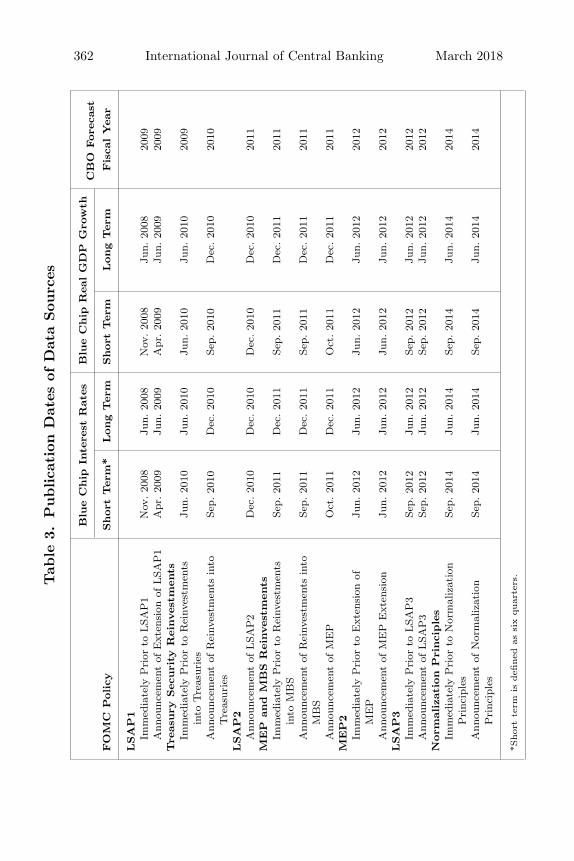
In addition to these assumptions, we need assumptions on inter-est rates and debt outstanding in order to construct the FederalReserve’s and the private sector’s holdings of Treasury securities interms of ten-year equivalents, with the private-sector holdings beingthe supply input for the term structure model. For interest rates,we rely on the Blue Chip Survey of Professional Forecasters fortheir views on the paths of the federal funds and ten-year Treasuryrates immediately before the implementation of the policy action weconsider. The five-year long-run annual projections from this datasource are released twice a year, in June and December. In addition,these projections include a five-year average for the selected variablesfor the years after the individual annual projections, resulting in aten-year projection. As a result, for policy interventions announcedin intervening months, we inspect the short-run projections thatcover six quarters into the future that are produced monthly andinterpolate these projections on a case-by-case basis, as describedin table 3. Furthermore, for each of the balance sheet scenarios, weproject total Treasury debt outstanding as well as the composition of
362 International Journal of Central Banking March 2018Tab
le3.
Publica
tion
Dat
esof
Dat
aSou
rces
Blu
eC
hip
Inte
rest
Rat
esB
lue
Chip
Rea
lG
DP
Gro
wth
CB
OFore
cast
FO
MC
Policy
Short
Ter
m*
Long
Ter
mShort
Ter
mLong
Ter
mFis
calY
ear
LSA
P1
Imm
edia
tely
Pri
orto
LSA
P1
Nov
.20
08Ju
n.20
08N
ov.20
08Ju
n.20
0820
09A
nnou
ncem
ent
ofE
xten
sion
ofLSA
P1
Apr
.20
09Ju
n.20
09A
pr.20
09Ju
n.20
0920
09Tre
asury
Sec
uri
tyR
einves
tmen
tsIm
med
iate
lyP
rior
toR
einv
estm
ents
into
Tre
asur
ies
Jun.
2010
Jun.
2010
Jun.
2010
Jun.
2010
2009
Ann
ounc
emen
tof
Rei
nves
tmen
tsin
toTre
asur
ies
Sep.
2010
Dec
.20
10Se
p.20
10D
ec.20
1020
10
LSA
P2
Ann
ounc
emen
tof
LSA
P2
Dec
.20
10D
ec.20
10D
ec.20
10D
ec.20
1020
11M
EP
and
MB
SR
einves
tmen
tsIm
med
iate
lyP
rior
toR
einv
estm
ents
into
MB
SSe
p.20
11D
ec.20
11Se
p.20
11D
ec.20
1120
11
Ann
ounc
emen
tof
Rei
nves
tmen
tsin
toM
BS
Sep.
2011
Dec
.20
11Se
p.20
11D
ec.20
1120
11
Ann
ounc
emen
tof
ME
PO
ct.20
11D
ec.20
11O
ct.20
11D
ec.20
1120
11M
EP
2Im
med
iate
lyP
rior
toE
xten
sion
ofM
EP
Jun.
2012
Jun.
2012
Jun.
2012
Jun.
2012
2012
Ann
ounc
emen
tof
ME
PE
xten
sion
Jun.
2012
Jun.
2012
Jun.
2012
Jun.
2012
2012
LSA
P3
Imm
edia
tely
Pri
orto
LSA
P3
Sep.
2012
Jun.
2012
Sep.
2012
Jun.
2012
2012
Ann
ounc
emen
tof
LSA
P3
Sep.
2012
Jun.
2012
Sep.
2012
Jun.
2012
2012
Norm
aliz
atio
nP
rinci
ple
sIm
med
iate
lyP
rior
toN
orm
aliz
atio
nP
rinc
iple
sSe
p.20
14Ju
n.20
14Se
p.20
14Ju
n.20
1420
14
Ann
ounc
emen
tof
Nor
mal
izat
ion
Pri
ncip
les
Sep.
2014
Jun.
2014
Sep.
2014
Jun.
2014
2014
*Shor
tte
rmis
defi
ned
assi
xqu
arte
rs.
Vol. 14 No. 2 Expectations about the Fed’s Balance Sheet 363
Treasury debt so we can project ten-year equivalents of both SOMAholdings and private-sector holdings. We use the Congressional Bud-get Office’s deficit forecast close to the time of the inception of theprogram to project Treasury debt outstanding. For the constructionof the maturity structure of Treasury debt, we rely on forecasts byWrightson Research for Treasury issuance, as well as policy state-ments by the Treasury on the expected evolution of the maturity ofTreasury debt over time.
4. The Effect of the Asset Programs
Given the models and assumptions outlined in section 3, we canconstruct the estimated term premium effect of each of the sevenprograms upon inception and at any other point of time. We illus-trate the main points using three different types of programs: thefirst asset purchase program, which represented a change in thesize and composition of the portfolio, with a calendar-based termi-nation date; the maturity extension program, which represented achange in only the composition of the portfolio; and the open-endedasset purchase program, which represented a change in the size andcomposition of the portfolio, but the termination date was tied tomacroeconomic outcomes and thus expectations for its ending couldchange over time. We compare our estimates to other studies, high-lighting different assumptions that can be responsible for variationsacross the estimates. Then we consider the term premium effect as ofNovember 2015 for all the programs and parse out the effect to thevarious programs. Finally, we discuss the confidence band aroundour estimates.
4.1 LSAP1: November 2008 and March 2009
Our first exercise demonstrates the use of our framework for a pro-gram that expands the Federal Reserve’s portfolio, changes its com-position, and has a known (even if updated) end date. The firstlarge-scale asset purchase program, announced in November 2008and expanded in March 2009, included purchases of $1.25 trillion ofagency MBS, about $175 billion of agency debt, and $300 billion in
364 International Journal of Central Banking March 2018
longer-dated Treasury securities.19 Markets reacted to the announce-ments of these programs. Upon the first announcement of the pro-gram, as documented in Gagnon et al. (2011), the ten-year Treasuryrate declined 7 basis points. The second announcement generatedan even larger 40 basis point decline in the ten-year Treasury rate.These reductions in the ten-year rate may have reflected changesin investors’ beliefs about the size and composition of the FederalReserve’s balance sheet, expectations for privately available secu-rities in the future, and general improvement in market function-ing. To estimate the TPE associated with LSAP1, we need twoSOMA projections—the counterfactual scenario where no LSAP1was implemented, and the scenario with LSAP1.20 The differencebetween the paths of SOMA holdings in these two scenarios repre-sents supposed supply shocks to private investors that were gener-ated by the LSAP1 program, i.e., the us path in our term premiummodel. Finally, we plug the us path into our model for the estimatedTPE.
4.1.1 LSAP1 Projection
The projection for the Federal Reserve’s balance sheet at the timewhen the first LSAP occurred is constructed using expectations forinterest rates and other key variables at the time of the implementa-tion of the program. It is helpful to remember that at the inceptionof LSAP1, the Committee stated that all purchases would be com-pleted by December 2009. As the program wore on, the Committeerevised its estimate to the first quarter of 2010 “in order to promotea smooth transition in markets.”21 As a result, the projections herereflect the earlier completion date of the LSAP1 program. Anotherassumption at the time of LSAP1 was that as the agency securities
19Holdings of agency MBS actually peaked at a lower level than the $1.25trillion, owing to prepayments on securities that were purchased earlier in theprogram.
20Projections for GDP, interest rates, and public debt use forecasts immediatelyprior to LSAP1.
21FOMC statement, December 19, 2009, available at http://www.federalreserve.gov/newsevents/press/monetary/20091216a.htm. This revision to theexpected end date of the purchases would be captured in the time-varying LSAPof this model if we reestimated the TPE at that juncture.
Vol. 14 No. 2 Expectations about the Fed’s Balance Sheet 365
prepaid or matured, these securities would roll off the portfolio, i.e.,there was no expectation of reinvestment at this time.
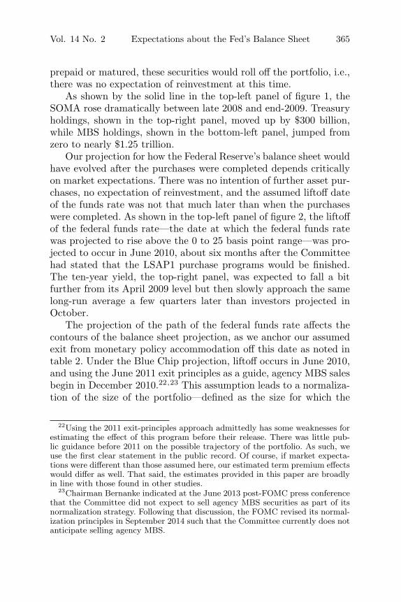
As shown by the solid line in the top-left panel of figure 1, theSOMA rose dramatically between late 2008 and end-2009. Treasuryholdings, shown in the top-right panel, moved up by $300 billion,while MBS holdings, shown in the bottom-left panel, jumped fromzero to nearly $1.25 trillion.
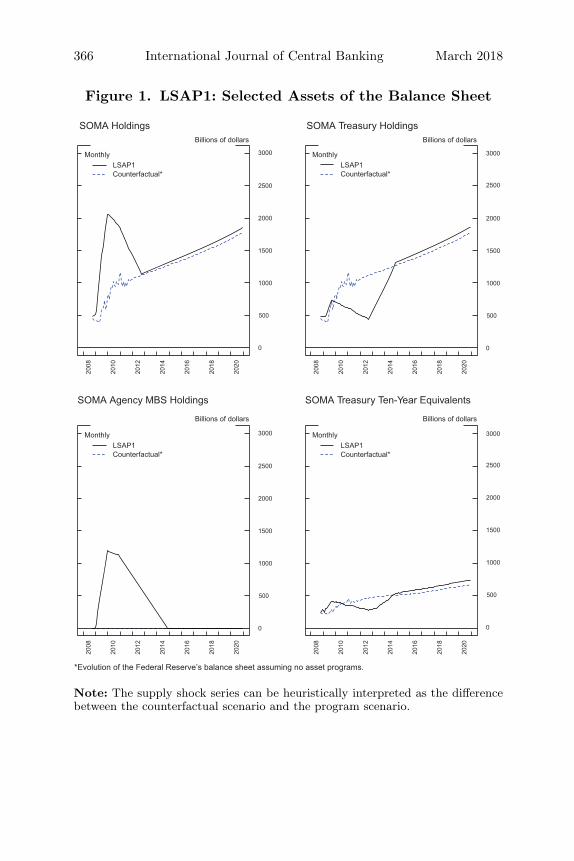
Our projection for how the Federal Reserve’s balance sheet wouldhave evolved after the purchases were completed depends criticallyon market expectations. There was no intention of further asset pur-chases, no expectation of reinvestment, and the assumed liftoff dateof the funds rate was not that much later than when the purchaseswere completed. As shown in the top-left panel of figure 2, the liftoffof the federal funds rate—the date at which the federal funds ratewas projected to rise above the 0 to 25 basis point range—was pro-jected to occur in June 2010, about six months after the Committeehad stated that the LSAP1 purchase programs would be finished.The ten-year yield, the top-right panel, was expected to fall a bitfurther from its April 2009 level but then slowly approach the samelong-run average a few quarters later than investors projected inOctober.
The projection of the path of the federal funds rate affects thecontours of the balance sheet projection, as we anchor our assumedexit from monetary policy accommodation off this date as noted intable 2. Under the Blue Chip projection, liftoff occurs in June 2010,and using the June 2011 exit principles as a guide, agency MBS salesbegin in December 2010.22,23 This assumption leads to a normaliza-tion of the size of the portfolio—defined as the size for which the
22Using the 2011 exit-principles approach admittedly has some weaknesses forestimating the effect of this program before their release. There was little pub-lic guidance before 2011 on the possible trajectory of the portfolio. As such, weuse the first clear statement in the public record. Of course, if market expecta-tions were different than those assumed here, our estimated term premium effectswould differ as well. That said, the estimates provided in this paper are broadlyin line with those found in other studies.
23Chairman Bernanke indicated at the June 2013 post-FOMC press conferencethat the Committee did not expect to sell agency MBS securities as part of itsnormalization strategy. Following that discussion, the FOMC revised its normal-ization principles in September 2014 such that the Committee currently does notanticipate selling agency MBS.
366 International Journal of Central Banking March 2018
Figure 1. LSAP1: Selected Assets of the Balance Sheet
Monthly LSAP1
Counterfactual*
Monthly LSAP1
Counterfactual*
Monthly LSAP1
Counterfactual*
Monthly LSAP1
Counterfactual*
SOMA Holdings Billions of dollars
3000
SOMA Treasury Holdings Billions of dollars
3000
2500 2500
2000 2000
1500 1500
1000 1000
500 500
0 0
SOMA Agency MBS Holdings
Billions of dollars
3000
SOMA Treasury Ten-Year Equivalents
Billions of dollars
3000
2500 2500
2000 2000
1500 1500
1000 1000
500 500
0 0
*Evolution of the Federal Reserve’s balance sheet assuming no asset programs.
2008
20
08
2010
20
10
2012
20
12
2014
20
14
2016
20
16
2018
20
18
2020
20
20
2008
20
08
2010
20
10
2012
20
12
2014
20
14
2016
20
16
2018
20
18
2020
20
20
Note: The supply shock series can be heuristically interpreted as the differencebetween the counterfactual scenario and the program scenario.
Vol. 14 No. 2 Expectations about the Fed’s Balance Sheet 367
Figure 2. LSAP1: Interest Rates
Quarterly LSAP1
Counterfactual*
Quarterly LSAP1
Counterfactual*
QuarterlyLSAP1
Federal Funds Rate percent
7
Ten-Year Treasury Rate percent
7
6
6
5
54
3 4
2
3
1
0 2
Term Premium Effect basis points
0
−10
−20
−30
−40
−50
2009 2010 2011 2012 2013 2014 2015 2016 2017 2018 2019 2020
2010
2012
2014
2016
2018
2020
2010
2012
2014
2016
2018
2020
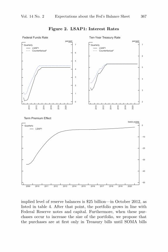
implied level of reserve balances is $25 billion—in October 2012, aslisted in table 4. After that point, the portfolio grows in line withFederal Reserve notes and capital. Furthermore, when these pur-chases occur to increase the size of the portfolio, we propose thatthe purchases are at first only in Treasury bills until SOMA bills
368 International Journal of Central Banking March 2018
Table 4. Dates for Key Balance Sheet Projections
Treasury BillsReserves = Are One-Third
FOMC Policy Date $25 Billion MBS = 0 of Portfolio
LSAP1 Apr. 2009 Oct. 2012 Nov. 2014 Apr. 2013Reinvestments into
Treasury SecuritiesSep. 2010 Jun. 2013 Nov. 2015 Feb. 2014
LSAP2 Nov. 2010 Jan. 2015 May 2016 Dec. 2015Reinvestment into
Agency MBSSecurities
Sep. 2011 Apr. 2016 Mar. 2018 Feb. 2017
MEP Sep. 2011 Jan. 2017 Mar. 2018 Jan. 2018Extended MEP Jun. 2012 Aug. 2017 May 2018 Aug. 2018LSAP3 Sep. 2012 Sep. 2018 Feb. 2019 Aug. 2019Normalization
PrinciplesSep. 2014 N/A* N/A* N/A*
*Occurs outside of the projection horizon.
reach one-third of total Treasury securities held in the portfolio—roughly in line with the composition of the portfolio before the startof the financial crisis. Once this ratio of one-third bills, two-thirdnotes and bonds is reached, purchases continue so that this ratiostays constant. These assumptions are embedded in the projectionsshown in figure 1.
Putting the interest rate paths together with SOMA Treasuryholdings gives us a path for SOMA Treasury ten-year equivalents,shown in the bottom-right panel of figure 1. This ten-year equiva-lents path and SOMA MBS (par value) holdings are the two inputsinto the term premium model for LSAP1.
4.1.2 LSAP1 Counterfactual
To estimate the TPE associated with LSAP1, we need to look at howmuch larger projected SOMA holdings were with the asset purchases(LSAP1 projection) than in a scenario where no LSAP1 was imple-mented (LSAP1 counterfactual). In this counterfactual scenario weassume a counterfactual scenario that is close to what was expectedby Blue Chip forecasters immediately prior to LSAP1. At that time,as indicated by the forecasters’ projections, they assumed a quick
Vol. 14 No. 2 Expectations about the Fed’s Balance Sheet 369
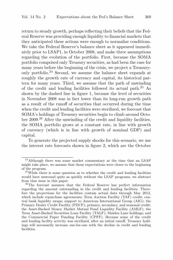
return to steady growth, perhaps reflecting their beliefs that the Fed-eral Reserve was providing enough liquidity to financial markets thatthey anticipated these actions were enough to normalize conditions.We take the Federal Reserve’s balance sheet as it appeared immedi-ately prior to LSAP1, in October 2008, and make three assumptionsregarding the evolution of the portfolio. First, because the SOMAportfolio comprised only Treasury securities, as had been the case formany years before the beginning of the crisis, we project a Treasury-only portfolio.24 Second, we assume the balance sheet expands atroughly the growth rate of currency and capital, its historical pat-tern for many years. Third, we assume that the path of unwindingof the credit and lending facilities followed its actual path.25 Asshown by the dashed line in figure 1, because the level of securitiesin November 2008 was in fact lower than its long-run growth pathas a result of the runoff of securities that occurred during the timewhen the credit and lending facilities were sterilized, we forecast thatSOMA’s holdings of Treasury securities begin to climb around Octo-ber 2009.26 After the unwinding of the credit and liquidity facilities,the SOMA portfolio grows at a constant rate, in line with growthof currency (which is in line with growth of nominal GDP) andcapital.
To generate the projected supply shocks for this scenario, we usethe interest rate forecasts shown in figure 2, which are the October
24Although there was some market commentary at the time that an LSAPmight take place, we assume that those expectations were closer to the beginningof the program.
25While there is some question as to whether the credit and lending facilitieswould have unwound quite as quickly without the LSAP programs, we abstractfrom that issue in this paper.
26The forecast assumes that the Federal Reserve has perfect informationregarding the amount outstanding in the credit and lending facilities. There-fore the projections for the facilities contain actual data through May 2012,which include repurchase agreements; Term Auction Facility (TAF) credit; cen-tral bank liquidity swaps; support to American International Group (AIG); thePrimary Dealer Credit Facility (PDCF); primary, secondary, and seasonal credit;the Asset-Backed Money Market Mutual Fund Liquidity Facility (AMLF); theTerm Asset-Backed Securities Loan Facility (TALF); Maiden Lane holdings; andthe Commercial Paper Funding Facility (CPFF). Because some of the creditand lending facility activity was sterilized, after an initial runoff, Treasury hold-ings will necessarily increase one-for-one with the decline in credit and lendingfacilities.
370 International Journal of Central Banking March 2018
2008 and June 2008 Blue Chip forecasts for the near term (six quar-ters) and longer term, respectively. The target federal funds ratewas expected to decline 25 basis points from its level at the time,and bottom out at 1 percent. The funds rate was then expected toclimb steadily to about 4.5 percent, near its long-run average andsomewhat lower than it had been immediately preceding the crisis.As shown in the top-right panel, the ten-year rate was expected toclimb as well, reaching a long-run value of about 5.25 percent by theend of 2012. Using these interest rates with the projected SOMATreasury holdings path, the SOMA Treasury ten-year equivalentsprojection is shown in the bottom-right panel of figure 1.
4.1.3 LSAP1 Term Premium Effect
With the LSAP1 and LSAP1 counterfactual projections, we can con-struct our supply shocks for our TPE model as the counterfactualvalue minus the LSAP1 value for both SOMA MBS holdings andSOMA Treasury ten-year equivalents, displayed in the bottom pan-els of figure 1. Since the Federal Reserve never held MBS prior tothe financial crisis, the projected value of uMBS is just the negativeof the amount of Federal Reserve holdings normalized by nominalGDP. For Treasury ten-year equivalents, one can see that projectedTreasury holdings are actually lower in the LSAP1 scenario thanthose in the counterfactual from mid-2010 through mid-2014, reflect-ing the fact that LSAP1’s purchases of MBS holdings boost theSOMA value, and Treasury holdings are not needed to offset growthin currency and capital. Looking at the long run, actual currencygrowth was much faster than what would have been projected inOctober 2008—likely a result of precautionary demand for dollar-denominated bank notes. Consequently, the balance sheet is perma-nently larger in the LSAP1 scenario than in the counterfactual.
As shown in the bottom panel of figure 2 and reported in row1, column 1 of table 5, the initial impact of the LSAP1 programwas to push down the ten-year Treasury yield by about 35 basispoints. This estimate is almost identical to the announcement effectbased on event studies, as discussed above, and our estimate is cer-tainly well within confidence bands around other studies’ estimates,as reported in table 6. In particular, D’Amico and King (2013) reporta 20 basis point decline attributable to the Treasury portion of the
Vol. 14 No. 2 Expectations about the Fed’s Balance Sheet 371
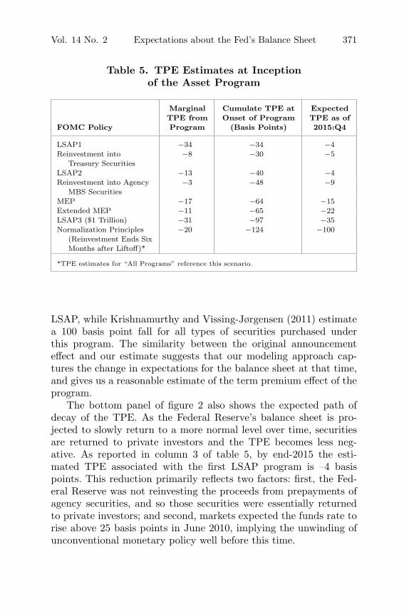
Table 5. TPE Estimates at Inceptionof the Asset Program
Marginal Cumulate TPE at ExpectedTPE from Onset of Program TPE as of
FOMC Policy Program (Basis Points) 2015:Q4
LSAP1 −34 −34 −4Reinvestment into
Treasury Securities−8 −30 −5
LSAP2 −13 −40 −4Reinvestment into Agency
MBS Securities−3 −48 −9
MEP −17 −64 −15Extended MEP −11 −65 −22LSAP3 ($1 Trillion) −31 −97 −35Normalization Principles
(Reinvestment Ends SixMonths after Liftoff)*
−20 −124 −100
*TPE estimates for “All Programs” reference this scenario.
LSAP, while Krishnamurthy and Vissing-Jørgensen (2011) estimatea 100 basis point fall for all types of securities purchased underthis program. The similarity between the original announcementeffect and our estimate suggests that our modeling approach cap-tures the change in expectations for the balance sheet at that time,and gives us a reasonable estimate of the term premium effect of theprogram.
The bottom panel of figure 2 also shows the expected path ofdecay of the TPE. As the Federal Reserve’s balance sheet is pro-jected to slowly return to a more normal level over time, securitiesare returned to private investors and the TPE becomes less neg-ative. As reported in column 3 of table 5, by end-2015 the esti-mated TPE associated with the first LSAP program is –4 basispoints. This reduction primarily reflects two factors: first, the Fed-eral Reserve was not reinvesting the proceeds from prepayments ofagency securities, and so those securities were essentially returnedto private investors; and second, markets expected the funds rate torise above 25 basis points in June 2010, implying the unwinding ofunconventional monetary policy well before this time.
372 International Journal of Central Banking March 2018
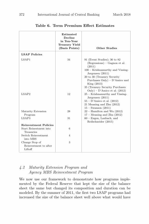
Table 6. Term Premium Effect Estimates
EstimatedDecline
in Ten-YearTreasury Yield(Basis Points) Other Studies
LSAP Policies
LSAP1 34 91 (Event Studies); 36 to 82(Regressions) – Gagnon et al.(2011)
100 – Krishnamurthy and Vissing-Jørgensen (2011)
20 to 30 (Treasury SecurityPurchases Only) – D’Amico andKing (2013)
35 (Treasury Security PurchasesOnly) – D’Amico et al. (2012)
LSAP2 12 25 – Krishnamurthy and Vissing-Jørgensen (2011)
55 – D’Amico et al. (2012)21 Meaning and Zhu (2012)15 – Swanson (2011)
Maturity ExtensionProgram
28 22 – Hamilton and Wu (2012)17 – Meaning and Zhu (2012)
LSAP3 31 60 – Engen, Laubach, andReifschneider (2015)
Reinvestment PoliciesStart Reinestment into
Treasuries6
Switch Reinvestmentinto MBS
4
Change Stop ofReinvestment to afterLiftoff
3
4.2 Maturity Extension Program andAgency MBS Reinvestment Program
We now use our framework to demonstrate how programs imple-mented by the Federal Reserve that kept the size of the balancesheet the same but changed its composition and duration can bemodeled. By the summer of 2011, the first two LSAP programs hadincreased the size of the balance sheet well above what would have
Vol. 14 No. 2 Expectations about the Fed’s Balance Sheet 373
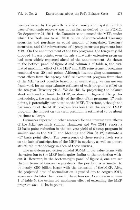
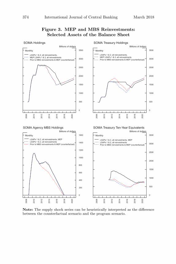
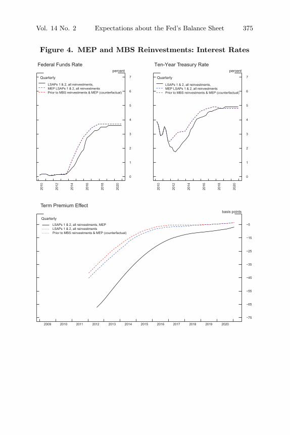
been expected by the growth rate of currency and capital, but thepace of economic recovery was not as fast as desired by the FOMC.On September 21, 2011, the Committee announced the MEP, underwhich the Desk was to sell $400 billion of shorter-dated Treasurysecurities and purchase an equal amount of long-dated Treasurysecurities, and the reinvestment of agency securities payments intoMBS. On the announcement of the two programs, the ten-year yielddropped 7 basis points, even though a maturity extension programhad been widely expected ahead of the announcement. As shownin the bottom panel of figure 3 and column 1 of table 5, the esti-mated maximum effect of the MEP and MBS reinvestment programscombined was –20 basis points. Although disentangling an announce-ment effect from the agency MBS reinvestment program from thatof the MEP is not possible based on an event study, we can use ourframework for an approximate estimate of each program’s effect onthe ten-year Treasury yield. We do this by projecting the balancesheet with and without the MEP, as shown in figure 4. Using thismethodology, the vast majority of the effect of the programs, 17 basispoints, is potentially attributed to the MEP. Therefore, although thepar amount of the MEP program was less than the second LSAPprogram, the impact on the term premium is estimated to be about1/2 times as large.
Estimates reported in other research for the interest rate effectsof the MEP are fairly similar. Hamilton and Wu (2012) report a22 basis point reduction in the ten-year yield of a swap program insimilar size as the MEP, and Meaning and Zhu (2012) estimate a–17 basis point effect. The convergence of these results likely restson the lack of anticipation of the MEP in markets, as well as a morestructured methodology in each of these studies.
The near-term projection of total SOMA in par value terms withthe extension to the MEP looks quite similar to the projection with-out it. However, in the bottom-right panel of figure 4, one can seethat in terms of ten-year equivalents, the portfolio is estimated tobe nearly $306 billion larger with the extension of the MEP. Also,the projected date of normalization is pushed out to August 2017,seven months later than prior to the extension. As shown in column1 of table 5, the estimated maximum effect of extending the MEPprogram was –11 basis points.
374 International Journal of Central Banking March 2018
Figure 3. MEP and MBS Reinvestments:Selected Assets of the Balance Sheet
Monthly
LSAPs 1 & 2, all reinvestments, MEP LSAPs 1 & 2, all reinvestments
Prior to MBS reinvestments & MEP (counterfactual)
Monthly
LSAPs 1 & 2, all reinvestments, MEP LSAPs 1 & 2, all reinvestments Prior to MBS reinvestments & MEP (counterfactual)
Monthly
LSAPs 1 & 2, all reinvestments, MEP LSAPs 1 & 2, all reinvestments
Prior to MBS reinvestments & MEP (counterfactual)
Monthly
LSAPs 1 & 2, all reinvestments, MEP LSAPs 1 & 2, all reinvestmentsPrior to MBS reinvestments & MEP (counterfactual)
SOMA Holdings Billions of dollars
3500
SOMA Treasury Holdings Billions of dollars
3500
3000 3000
2500 2500
2000 2000
1500 1500
1000 1000
500 500
0 0
SOMA Agency MBS Holdings Billions of dollars
1600
SOMA Treasury Ten-Year Equivalents Billions of dollars
3500
1400 3000
1200 2500
1000 2000
800
6001500
4001000
200 500
0 0
2008
20
08
2010
20
10
2012
20
12
2014
20
14
2016
20
16
2018
20
18
2020
20
20
2008
20
08
2010
20
10
2012
20
12
2014
20
14
2016
20
16
2018
20
18
2020
20
20
Note: The supply shock series can be heuristically interpreted as the differencebetween the counterfactual scenario and the program scenario.
Vol. 14 No. 2 Expectations about the Fed’s Balance Sheet 375
Figure 4. MEP and MBS Reinvestments: Interest Rates
Quarterly
LSAPs 1 & 2, all reinvestments, MEP LSAPs 1 & 2, all reinvestments
Prior to MBS reinvestments & MEP (counterfactual)
Quarterly
LSAPs 1 & 2, all reinvestments, MEP LSAPs 1 & 2, all reinvestments Prior to MBS reinvestments & MEP (counterfactual)
Quarterly LSAPs 1 & 2, all reinvestments, MEP
LSAPs 1 & 2, all reinvestments Prior to MBS reinvestments & MEP (counterfactual)
Federal Funds Rate percent
7
Ten-Year Treasury Rate percent
7
6 6
5 5
4 4
3 3
2 2
1 1
0 0
Term Premium Effect basis points
−5
−15
−25
−35
−45
−55
−65
−75
2009 2010 2011 2012 2013 2014 2015 2016 2017 2018 2019 2020
2010
2012
2014
2016
2018
2020
2010
2012
2014
2016
2018
2020
376 International Journal of Central Banking March 2018
4.3 LSAP3: September 2012
Our third exercise demonstrates how changes in expectations aboutthe macroeconomy and Federal Reserve policy can alter the effects ofa program. On September 13, 2012 the FOMC released its statementfollowing the scheduled September policy meeting. The statementannounced the third round of large-scale asset purchases by stating:“the Committee agreed today to increase policy accommodation bypurchasing additional agency mortgage-backed securities at a pace of$40 billion per month. . . . These actions, which together will increasethe Committee’s holdings of longer-term securities by about $85 bil-lion each month. . . should put downward pressure on longer-terminterest rates.” This statement incorporated the purchases includedunder the ongoing MEP program of $45 billion per month, whichwas scheduled to run through December. After the December FOMCmeeting, the Committee released its statement stating “the Com-mittee will continue purchasing additional agency mortgage-backedsecurities at a pace of $40 billion per month. The Committee alsowill purchase longer-term Treasury securities . . . initially at a paceof $45 billion per month.” This continuation of Treasury asset pur-chases beyond the extension of the MEP marked the beginning ofthe full-scale LSAP3 asset purchase program.
Unlike LSAP1 and LSAP2, LSAP3 was announced as an open-ended program with no set size for the total amount of purchases. Forour assumptions on the amount of purchases the market expected,we use the primary dealer survey released after the announcementof the program in September 2012. According to those reported esti-mates, which we assume for our projection, purchases were expectedto commence in the month following the FOMC announcement(October 2012) and continue that pace through the end of 2013before ceasing. Moreover, at the time of the announcement of theprogram, the Committee had maintained its commitment to sellagency MBS as part of the policy normalization process. Total pur-chases in our projection are $520 billion of MBS and $540 billion ofTreasury securities. The actual size of the program far exceeds thisamount.27 The counterfactual for this program uses the Blue Chip
27In the September 2012 primary dealer survey, some dealers did indicate theyexpected a taper of asset purchases before the end of the program, but this wasnot a dominant view.
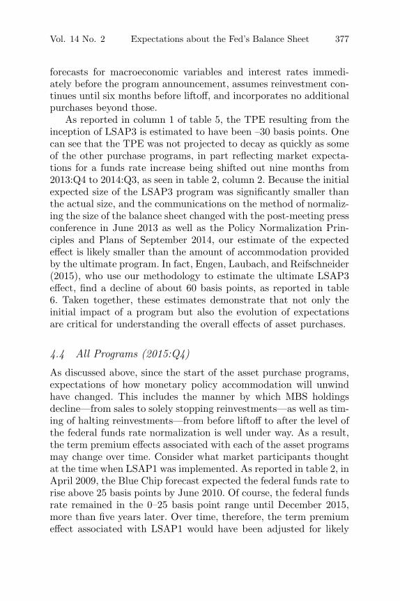
Vol. 14 No. 2 Expectations about the Fed’s Balance Sheet 377
forecasts for macroeconomic variables and interest rates immedi-ately before the program announcement, assumes reinvestment con-tinues until six months before liftoff, and incorporates no additionalpurchases beyond those.
As reported in column 1 of table 5, the TPE resulting from theinception of LSAP3 is estimated to have been –30 basis points. Onecan see that the TPE was not projected to decay as quickly as someof the other purchase programs, in part reflecting market expecta-tions for a funds rate increase being shifted out nine months from2013:Q4 to 2014:Q3, as seen in table 2, column 2. Because the initialexpected size of the LSAP3 program was significantly smaller thanthe actual size, and the communications on the method of normaliz-ing the size of the balance sheet changed with the post-meeting pressconference in June 2013 as well as the Policy Normalization Prin-ciples and Plans of September 2014, our estimate of the expectedeffect is likely smaller than the amount of accommodation providedby the ultimate program. In fact, Engen, Laubach, and Reifschneider(2015), who use our methodology to estimate the ultimate LSAP3effect, find a decline of about 60 basis points, as reported in table6. Taken together, these estimates demonstrate that not only theinitial impact of a program but also the evolution of expectationsare critical for understanding the overall effects of asset purchases.
4.4 All Programs (2015:Q4)
As discussed above, since the start of the asset purchase programs,expectations of how monetary policy accommodation will unwindhave changed. This includes the manner by which MBS holdingsdecline—from sales to solely stopping reinvestments—as well as tim-ing of halting reinvestments—from before liftoff to after the level ofthe federal funds rate normalization is well under way. As a result,the term premium effects associated with each of the asset programsmay change over time. Consider what market participants thoughtat the time when LSAP1 was implemented. As reported in table 2, inApril 2009, the Blue Chip forecast expected the federal funds rate torise above 25 basis points by June 2010. Of course, the federal fundsrate remained in the 0–25 basis point range until December 2015,more than five years later. Over time, therefore, the term premiumeffect associated with LSAP1 would have been adjusted for likely
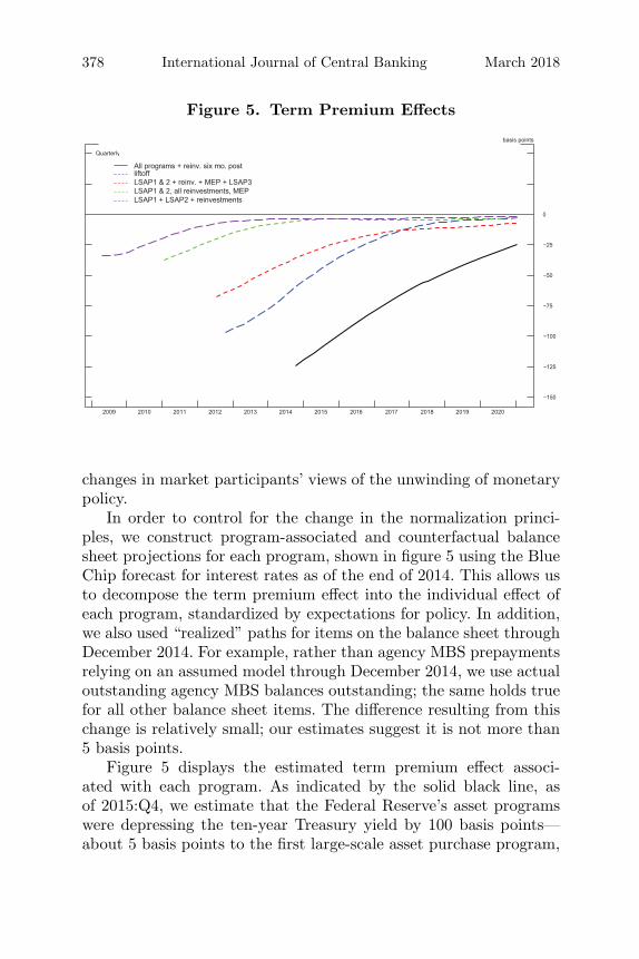
378 International Journal of Central Banking March 2018
Figure 5. Term Premium Effects
basis points
0
−25
−50
−75
−100
−125
−150
2009 2010 2011 2012 2013 2014 2015 2016 2017 2018 2019 2020
Quarterly
All programs + reinv. six mo. post liftoff LSAP1 & 2 + reinv. + MEP + LSAP3 LSAP1 & 2, all reinvestments, MEP LSAP1 + LSAP2 + reinvestments
changes in market participants’ views of the unwinding of monetarypolicy.
In order to control for the change in the normalization princi-ples, we construct program-associated and counterfactual balancesheet projections for each program, shown in figure 5 using the BlueChip forecast for interest rates as of the end of 2014. This allows usto decompose the term premium effect into the individual effect ofeach program, standardized by expectations for policy. In addition,we also used “realized” paths for items on the balance sheet throughDecember 2014. For example, rather than agency MBS prepaymentsrelying on an assumed model through December 2014, we use actualoutstanding agency MBS balances outstanding; the same holds truefor all other balance sheet items. The difference resulting from thischange is relatively small; our estimates suggest it is not more than5 basis points.
Figure 5 displays the estimated term premium effect associ-ated with each program. As indicated by the solid black line, asof 2015:Q4, we estimate that the Federal Reserve’s asset programswere depressing the ten-year Treasury yield by 100 basis points—about 5 basis points to the first large-scale asset purchase program,
Vol. 14 No. 2 Expectations about the Fed’s Balance Sheet 379
a negligible amount to the second, about 20 basis points each tothe maturity extension program and its continuation, a little over20 basis points to the third, and the remainder to the reinvestmentprograms. Although one of the main drivers in differences of the pro-grams is the change in expectations regarding interest rates, thereare also differences that result from using realized balance sheetquantities instead of projected ones. For example, the projection atthe time of LSAP1 had much slower agency MBS prepayments thanwhat actually occurred, as interest rates declined much more thanwhat was expected at the time of the implementation of LSAP1.Consequently, the realized term premium effect was likely a bitsmaller than the projected term premium effect at the inceptionof the program.
To summarize, the yield on the ten-year Treasury has fallenabout 150 basis points since the start of the LSAP1 program.Although there have been many factors that have affected yieldsfrom 2008:Q4 to 2015:Q4, we would potentially attribute slightlyless than two-thirds of the drop to the asset programs by the FederalReserve.
4.5 Confidence Bands around the Estimates
Our TPE estimate depends critically on the assumed path of howthe Federal Reserve’s unconventional monetary policy is expected tounwind and, hence, how the net supply of assets return back to pri-vate investors. It also depends importantly on the model we use andthe parameter estimates. To explore one aspect of the uncertaintyaround our estimate, figure 6 presents the 90 percent confidenceinterval around the point estimate for the cumulative effect of allthe programs, which captures the sampling uncertainty for a givenmodel and given balance sheet paths.28 As can be seen in the figure,the confidence interval suggests that the TPE effect could have beenas large as 140 basis points or as small as 56 basis points. Theseconfidence bands are in line with the literature on asset purchases,
28We use a delta method on the term premium effect (TPE) equation (10)together with estimated standard errors of model parameters to calculate thestandard errors of the TPE estimates. The 90 percent confidence interval of theTPE estimates is then calculated assuming that the model parameters and thusTPE estimates are normally distributed.
380 International Journal of Central Banking March 2018
Figure 6. Effect of Balance Sheet Operations on theTen-Year Treasury Term Premium
Quarterly basis points
0 0
−20 −20
−40 −40
−60 −60
−80 −80
−100 −100
−120 −120
−140 −140
−160 −160
2015 2016 2017 2018 2019 2020
Source: Li and Wei (2013) and Ihrig et al. (2015).Note: Shaded area indicates a 90 percent confidence interval for the cumulativeeffect of all programs beginning in 2015:Q4.
suggesting that our estimates are potentially in line with a range ofother methodologies.
5. Conclusion
This paper provides a novel application of a term structure modelthat includes supply effects to evaluate the effect of the FederalReserve’s recent unconventional monetary policy on interest ratesboth at inception and over time. Overall, our results suggest thata large portion of the decline in interest rates from April 2009 toOctober 2014 may be attributed to the Federal Reserve’s asset pro-grams. And, as of this writing, there remains notable downwardpressure on Treasury yields from unconventional policies taken sev-eral years ago. We highlight the importance of expectations of theFederal Reserve’s balance sheet and of interest rates on the impactof the asset programs, as well as the necessity of careful applicationof an implied Federal Reserve portfolio strategy to calculating theseeffects.
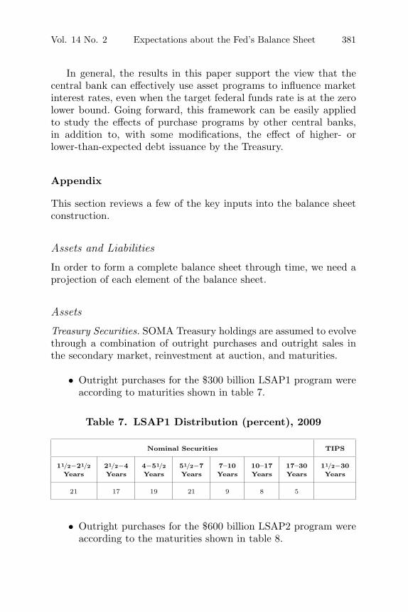
Vol. 14 No. 2 Expectations about the Fed’s Balance Sheet 381
In general, the results in this paper support the view that thecentral bank can effectively use asset programs to influence marketinterest rates, even when the target federal funds rate is at the zerolower bound. Going forward, this framework can be easily appliedto study the effects of purchase programs by other central banks,in addition to, with some modifications, the effect of higher- orlower-than-expected debt issuance by the Treasury.
Appendix
This section reviews a few of the key inputs into the balance sheetconstruction.
Assets and Liabilities
In order to form a complete balance sheet through time, we need aprojection of each element of the balance sheet.
Assets
Treasury Securities. SOMA Treasury holdings are assumed to evolvethrough a combination of outright purchases and outright sales inthe secondary market, reinvestment at auction, and maturities.
• Outright purchases for the $300 billion LSAP1 program wereaccording to maturities shown in table 7.
Table 7. LSAP1 Distribution (percent), 2009
Nominal Securities TIPS
11/2−21/2 21/2−4 4−51/2 51/2−7 7–10 10–17 17–30 11/2−30Years Years Years Years Years Years Years Years
21 17 19 21 9 8 5
• Outright purchases for the $600 billion LSAP2 program wereaccording to the maturities shown in table 8.
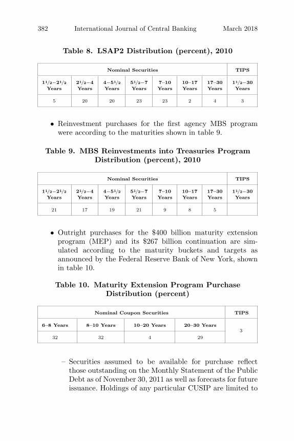
382 International Journal of Central Banking March 2018
Table 8. LSAP2 Distribution (percent), 2010
Nominal Securities TIPS
11/2−21/2 21/2−4 4−51/2 51/2−7 7–10 10–17 17–30 11/2−30Years Years Years Years Years Years Years Years
5 20 20 23 23 2 4 3
• Reinvestment purchases for the first agency MBS programwere according to the maturities shown in table 9.
Table 9. MBS Reinvestments into Treasuries ProgramDistribution (percent), 2010
Nominal Securities TIPS
11/2−21/2 21/2−4 4−51/2 51/2−7 7–10 10–17 17–30 11/2−30Years Years Years Years Years Years Years Years
21 17 19 21 9 8 5
• Outright purchases for the $400 billion maturity extensionprogram (MEP) and its $267 billion continuation are sim-ulated according to the maturity buckets and targets asannounced by the Federal Reserve Bank of New York, shownin table 10.
Table 10. Maturity Extension Program PurchaseDistribution (percent)
Nominal Coupon Securities TIPS
6–8 Years 8–10 Years 10–20 Years 20–30 Years3
32 32 4 29
– Securities assumed to be available for purchase reflectthose outstanding on the Monthly Statement of the PublicDebt as of November 30, 2011 as well as forecasts for futureissuance. Holdings of any particular CUSIP are limited to
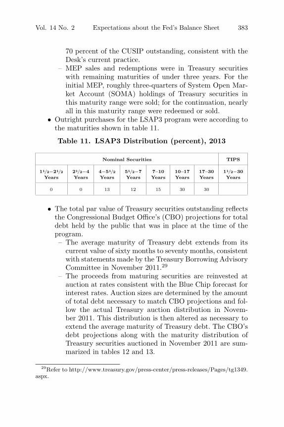
Vol. 14 No. 2 Expectations about the Fed’s Balance Sheet 383
70 percent of the CUSIP outstanding, consistent with theDesk’s current practice.
– MEP sales and redemptions were in Treasury securitieswith remaining maturities of under three years. For theinitial MEP, roughly three-quarters of System Open Mar-ket Account (SOMA) holdings of Treasury securities inthis maturity range were sold; for the continuation, nearlyall in this maturity range were redeemed or sold.
• Outright purchases for the LSAP3 program were according tothe maturities shown in table 11.
Table 11. LSAP3 Distribution (percent), 2013
Nominal Securities TIPS
11/2−21/2 21/2−4 4−51/2 51/2−7 7–10 10–17 17–30 11/2−30Years Years Years Years Years Years Years Years
0 0 13 12 15 30 30
• The total par value of Treasury securities outstanding reflectsthe Congressional Budget Office’s (CBO) projections for totaldebt held by the public that was in place at the time of theprogram.– The average maturity of Treasury debt extends from its
current value of sixty months to seventy months, consistentwith statements made by the Treasury Borrowing AdvisoryCommittee in November 2011.29
– The proceeds from maturing securities are reinvested atauction at rates consistent with the Blue Chip forecast forinterest rates. Auction sizes are determined by the amountof total debt necessary to match CBO projections and fol-low the actual Treasury auction distribution in Novem-ber 2011. This distribution is then altered as necessary toextend the average maturity of Treasury debt. The CBO’sdebt projections along with the maturity distribution ofTreasury securities auctioned in November 2011 are sum-marized in tables 12 and 13.
29Refer to http://www.treasury.gov/press-center/press-releases/Pages/tg1349.aspx.
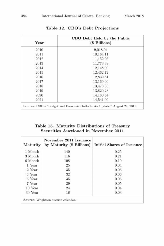
384 International Journal of Central Banking March 2018
Table 12. CBO’s Debt Projections
CBO Debt Held by the PublicYear ($ Billions)
2010 9,018.942011 10,164.112012 11,152.932013 11,773.392014 12,148.092015 12,462.722016 12,839.812017 13,169.092018 13,473.332019 13,820.232020 14,180.642021 14,541.09
Source: CBO’s “Budget and Economic Outlook: An Update,” August 24, 2011.
Table 13. Maturity Distributions of TreasurySecurities Auctioned in November 2011
November 2011 IssuanceMaturity by Maturity ($ Billions) Initial Shares of Issuance
1 Month 140 0.253 Month 116 0.216 Month 108 0.191 Year 25 0.042 Year 35 0.063 Year 32 0.065 Year 35 0.067 Year 29 0.0510 Year 24 0.0430 Year 16 0.03
Source: Wrightson auction calendar.
Vol. 14 No. 2 Expectations about the Fed’s Balance Sheet 385
Agency Securities. The agency securities portfolio is assumed toevolve due to a combination of purchases, sales, and prepayments.
• Consistent with the FOMC’s statement after the September2011 FOMC meeting, principal payments from SOMA agencyMBS and debt are reinvested in agency MBS. We use a cur-rent coupon model to estimate the coupon on newly purchasedMBS securities based on the consensus long-run Blue Chipforecast for the ten-year Treasury rate.
• Prepayments on settled agency MBS holdings are generatedby applying the realized prepayment rate on the SOMA hold-ings of MBS for historical values, then smoothed into a stan-dard prepayment rate for projected values. This prepaymentrate is calculated using a Richard and Roll (1989) prepaymentmodel, which assumes prepayments are a function of the ratioof the coupon rate on the agency MBS securities and the pre-vailing level of the mortgage rate. The higher this ratio, thefaster the prepayment speed.
• Prepayments on anticipated future purchases of agency MBSfollow the Richard and Roll (1989) model for the life of thesecurity.
• Under scenarios with securities sales, sales of agency securitiesbegin six months after the first increase in the federal fundsrate and last for four years. This timing is consistent withthat laid out in the June 2011 FOMC minutes; however, theexact timing is merely illustrative and chosen so as to be easilyimplementable in our projections.
• Under these assumptions, and given the maturity schedule foragency debt securities, the volume of sales necessary to reduceholdings of these securities to zero over the four-year periodonly requires a six-month period of minimal sales near the endof those four years.
Premiums and Discounts. A premium (discount) is the amountpaid above (below) the par value of a security. We use straight-lineamortization of these premiums and discounts over the expected lifeof current SOMA holdings. We derive new premiums and discountsfrom outright Treasury purchases by using the difference between

386 International Journal of Central Banking March 2018
the assumed coupon of the security being purchased and the corre-sponding market interest rate, as given by the yield-curve estimatesshown in table 14.30 We assume that agency MBS are purchased at aprice 2 percent above par value, and therefore book some premiumson these asset purchases.
Liabilities
Reserve Balances. Reserve balances are the residual of assets lessother liabilities less capital in the balance sheet projection. In gen-eral, increases in the level of Federal Reserve assets add reserve bal-ances. By contrast, increases in the levels of liability items, such asFederal Reserve notes in circulation or other liabilities, or increasesin the level of Reserve Bank capital, drain reserve balances.
A minimum level of $25 billion is set for reserve balances, roughlyequal to the level of reserve balances before the start of the finan-cial crisis. To maintain reserve balances at this level, first Treasurybills are purchased. Purchases of bills continue until these securitiescomprise one-third of the Federal Reserve’s total Treasury securityholdings—about the average level prior to the crisis. Once this levelis reached, the Federal Reserve buys notes and bonds in additionto bills to maintain an approximate composition of the portfolio ofone-third bills and two-thirds coupon securities.
Currency. Federal Reserve notes in circulation are assumed togrow at the same rate as nominal GDP. We use the consensus BlueChip forecasts for real GDP growth and the price level to form theforecast for nominal GDP growth. Because this is an annual fore-cast, we use the annual growth rate as the annualized quarterlygrowth rate for the second and third quarters of each year, and theninterpolate growth rates for the first and fourth quarters of the year.
30There is a slight inconsistency in our methodology: the yield curve used toprice securities purchases is different from the yield curve used to determine theterm premium effect of these purchases. No matter what, there would be someinconsistency between the two, unless we solved for a fixed point for the yieldchange (changes in the term premium affect the level of premiums, which thenaffects the size of the Federal Reserve’s balance sheet, which then affects the levelof the term premium). In addition, we only have Blue Chip projected rates toconstruct a forward-looking yield curve. To solve this problem, we use a simpleyield curve based on historical relationships between the federal funds rate, theten-year rate, and various tenors of the yield curve.
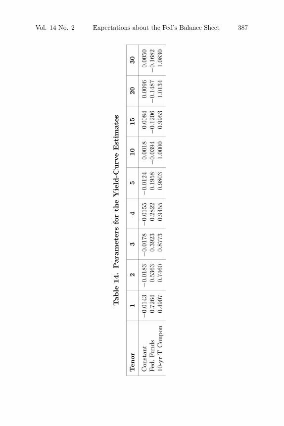
Vol. 14 No. 2 Expectations about the Fed’s Balance Sheet 387
Tab
le14
.Par
amet
ers
for
the
Yie
ld-C
urv
eEst
imat
es
Ten
or1
23
45
1015
2030
Con
stan
t−
0.01
43−
0.01
83−
0.01
78−
0.01
55−
0.01
240.
0018
0.00
840.
0096
0.00
50Fe
d.Fu
nds
0.72
640.
5363
0.39
230.
2822
0.19
58−
0.03
94−
0.12
06−
0.14
87−
0.16
8210
-yr
TC
oupo
n0.
4907
0.74
600.
8773
0.94
550.
9803
1.00
000.
9953
1.01
341.
0830
388 International Journal of Central Banking March 2018
Other Liabilities. The Federal Reserve conducts reverse repur-chases (RRPs) with foreign official and international accounts, andother counterparties. The volume of RRPs that is conducted withforeign official and international accounts is assumed to stay con-stant at its most recent historical monthly level, depending on theprojection period. The portion that is conducted with others isassumed to stay at zero over the projection period.
The Treasury General Account (TGA) cash balance is projectedto stay constant at $84 billion, which is the average level of the TGAsince the LSAP programs began through 2016:Q1.
We maintain the (Supervisory Formula Approach, SFA) balanceat its current level of zero throughout the forecast, consistent withthe Treasury Borrowing Advisory Committee’s recommendation notto resume the program at this time.31
Capital
Federal Reserve capital grows 15 percent per year, in line with theaverage rate of growth preceding the financial crisis.
References
Bauer, M. D., and G. D. Rudebusch. 2014. “The Signaling Channelfor Federal Reserve Bond Purchases.” International Journal ofCentral Banking 10 (3, September): 233–89.
Bernanke, B., and V. Reinhart. 2004. “Conducting Monetary Policyat Very Low Short-Term Interest Rates.” American EconomicReview 94 (2, May): 85–90.
Carpenter, S., J. Ihrig, E. Klee, D. Quinn, and A. Boote. 2015.“The Federal Reserve’s Balance Sheet: A Primer and Projec-tions.” International Journal of Central Banking 11 (2, March):237–84.
Christensen, J., J. Lopez, and G. Rudebusch. 2015. “A Probability-Based Stress Test of Federal Reserve Assets and Income.” Jour-nal of Monetary Economics 73 (July): 26–43.
31Refer to “Minutes of the Meeting of the Treasury Borrowing Advisory Com-mittee, the Securities Industry and Financial Markets Association, November1, 2011,” available for download at http://www.treasury.gov/press-center/press-releases/Pages/tg1349.aspx.
Vol. 14 No. 2 Expectations about the Fed’s Balance Sheet 389
Chung, H., J.-P. Laforte, D. Reifschneider, and J. C. Williams. 2011.“Estimating the Macroeconomic Effects of the Fed’s Asset Pur-chases.” FRBSF Economic Letter No. 2011-03 (January 31).
———. 2012. “Have We Underestimated the Likelihood and Sever-ity of Zero Lower Bound Events?” Journal of Money, Credit andBanking 44 (s1): 47–82.
D’Amico, S., W. English, D. Lopez-Salido, and E. Nelson. 2012.“The Federal Reserve’s Large-scale Asset Purchase Programmes:Rationale and Effects.” Economic Journal 122 (564): F415–F446.
D’Amico, S., and T. King. 2013. “Flow and Stock Effects of Large-Scale Treasury Purchases: Evidence on the Importance of LocalSupply.” Journal of Financial Economics 108 (2): 425–48.
Engen, E., T. Laubach, and D. Reifschneider. 2015. “The Macroeco-nomic Effects of the Federal Reserve’s Unconventional MonetaryPolicies.” FEDS Paper No. 2015-005 (January).
Gagnon, J., M. Raskin, J. Remache, and B. Sack. 2011. “TheFinancial Market Effects of the Federal Reserve’s Large-ScaleAsset Purchases.” International Journal of Central Banking 7(1, March): 3–43.
Greenlaw, D., J. D. Hamilton, P. Hooper, and F. S. Mishkin. 2013.“Crunch Time: Fiscal Crises and the Role of Monetary Policy.”NBER Working Paper No. 19297.
Greenwood, R., and D. Vayanos. 2014. “Bond Supply and ExcessBond Returns.” Review of Financial Studies 27 (3): 663–713.
Hamilton, J., and J. C. Wu. 2012. “The Effectiveness of AlternativeMonetary Policy Tools in a Zero Lower Bound Environment.”Journal of Money, Credit and Banking 44 (s1): 3–46.
Ihrig, J., E. E. Meade, and G. Weinbach. 2015. “Rewriting MonetaryPolicy 101: What’s the Fed’s Preferred Post-Crisis Approach toRaising Interest Rates?” Journal of Economic Perspectives 29(4, Fall): 177–98.
Krishnamurthy, A., and A. Vissing-Jørgensen. 2011. “The Effectsof Quantitative Easing on Interest Rates: Channels and Implica-tions for Policy.” Brookings Papers on Economic Activity (Fall):215–80.
Li, C., and M. Wei. 2013. “Term Structure Modeling with Sup-ply Factors and the Federal Reserve’s Large Scale Asset Pur-chase Programs.” International Journal of Central Banking 9(1, March): 3–39.
390 International Journal of Central Banking March 2018
Meaning, J., and F. Zhu. 2012. “The Impact of Federal Reserve AssetPurchase Programmes: Another Twist.” BIS Quarterly Review(March): 23–30.
Richard, S. F., and R. Roll. 1989. “Prepayments on Fixed-RateMortgage-Backed Securities.” Journal of Portfolio Management15 (3, Spring): 73–82.
Swanson, E. T. 2011. “Let’s Twist Again: A High-Frequency Event-Study Analysis of Operation Twist and Its Implications forQE2.” Brookings Papers on Economic Activity (Spring): 151–88.
Vayanos, D., and J.-L. Vila. 2009. “A Preferred-Habitat Model ofthe Term Structure of Interest Rates.” NBER Working PaperNo. 15487 (November).