PHYSICS 2240 Date: 9/27/2013

Experiment: 4

Kirchhoff’s Circuit Laws

Shabuktagin Photon Khan

Introduction

The objective of the experiment is to verify the laws for a resistive circuit using a DC input and

for a time varying RC circuit. Kirchhoff’s current law and Kirchhoff’s voltage law are verified

through “Y” circuit and RC circuit. The DC portion and the RC portion of the lab are each stand-

alone labs.

Theory

Kirchhoff’s Rules (sometimes called laws) state

1) Junction Rule: the total current flowing into any point is zero at all times where we use

the convention that current into a point is positive and current out of the point is negative.

This rule is also known as Kirchhoff’s current law. In other words, the algebraic sum of

all the currents at any node is zero.

(summation of current) ∑ I = 0 Equation: 1

2) Loop Rule: the sum of the voltage drops around any closed loop must equal zero where

the drop is negative if the voltage decreases and positive if the voltage increases in the

direction that one goes around the loop. This rule is also known Kirchhoff’s voltage law.

In other words, Kirchhoff’s voltage law states that the algebraic sum of all the voltages

around any closed path is zero.

(summation of voltage) ∑ V = 0 Equation: 2

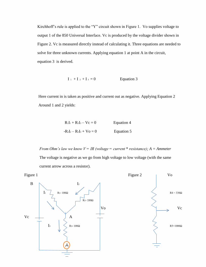
Kirchhoff’s rule is applied to the “Y” circuit shown in Figure 1. Vo supplies voltage to

output 1 of the 850 Universal Interface. Vc is produced by the voltage divider shown in

Figure 2. Vc is measured directly instead of calculating it. Three equations are needed to

solve for three unknown currents. Applying equation 1 at point A in the circuit,

equation 3 is derived.

I 1 + I 2 + I 3 = 0 Equation 3

Here current in is taken as positive and current out as negative. Applying Equation 2

Around 1 and 2 yields:

R1I1 + R3I3 – Vc = 0 Equation 4

-R2I2 – R3I3 + Vo = 0 Equation 5

From Ohm’s law we know V = IR (voltage = current * resistance); A = Ammeter

The voltage is negative as we go from high voltage to low voltage (with the same

current arrow across a resistor).

Figure 1 Figure 2 Vo

B I2

I1 R1= 100Ω R4 = 330Ω

R2= 330Ω

Vo Vc

Vc A

I3 R3= 100Ω R5=1000Ω

Experimental Procedure

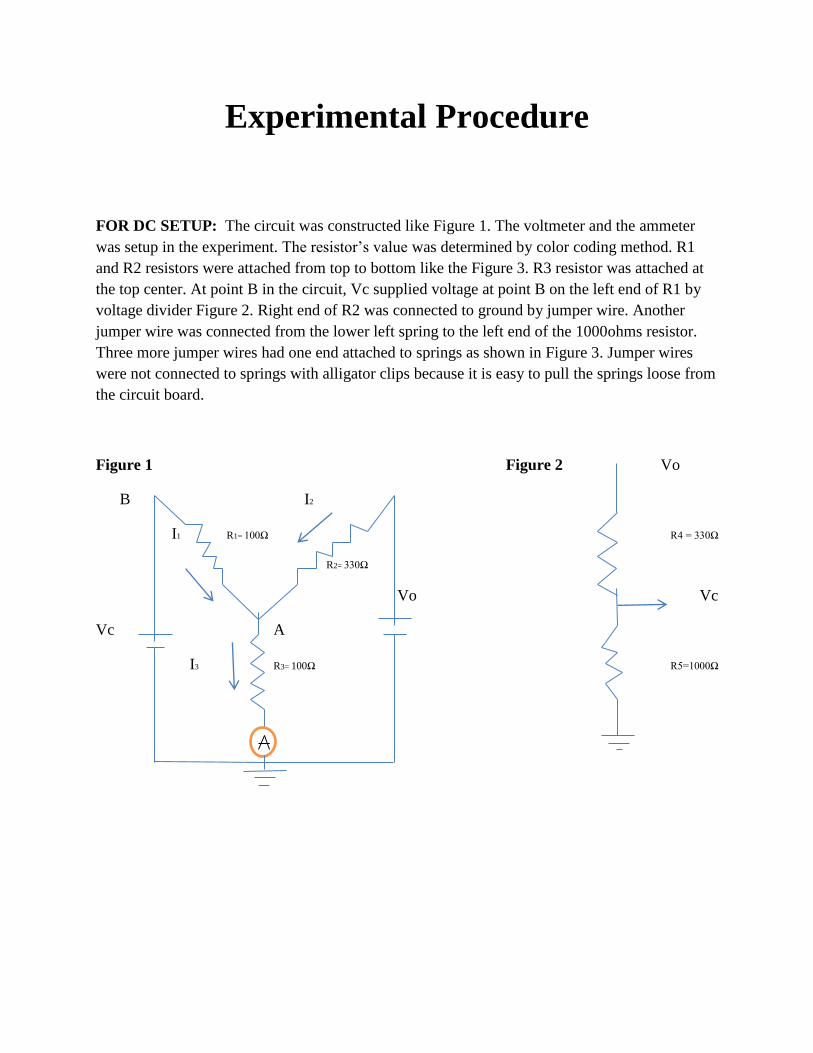
FOR DC SETUP: The circuit was constructed like Figure 1. The voltmeter and the ammeter

was setup in the experiment. The resistor’s value was determined by color coding method. R1

and R2 resistors were attached from top to bottom like the Figure 3. R3 resistor was attached at

the top center. At point B in the circuit, Vc supplied voltage at point B on the left end of R1 by

voltage divider Figure 2. Right end of R2 was connected to ground by jumper wire. Another

jumper wire was connected from the lower left spring to the left end of the 1000ohms resistor.

Three more jumper wires had one end attached to springs as shown in Figure 3. Jumper wires

were not connected to springs with alligator clips because it is easy to pull the springs loose from

the circuit board.

Figure 1 Figure 2 Vo

B I2

I1 R1= 100Ω R4 = 330Ω

R2= 330Ω

Vo Vc

Vc A

I3 R3= 100Ω R5=1000Ω

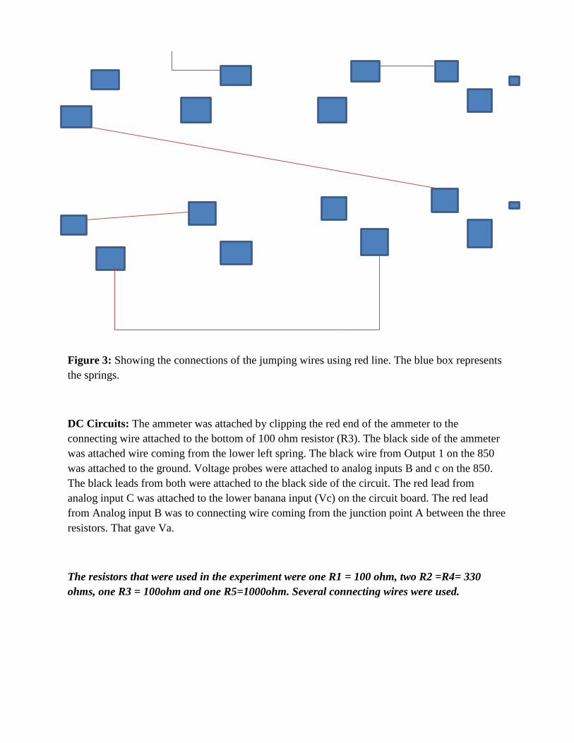
Figure 3: Showing the connections of the jumping wires using red line. The blue box represents

the springs.

DC Circuits: The ammeter was attached by clipping the red end of the ammeter to the

connecting wire attached to the bottom of 100 ohm resistor (R3). The black side of the ammeter

was attached wire coming from the lower left spring. The black wire from Output 1 on the 850

was attached to the ground. Voltage probes were attached to analog inputs B and c on the 850.

The black leads from both were attached to the black side of the circuit. The red lead from

analog input C was attached to the lower banana input (Vc) on the circuit board. The red lead

from Analog input B was to connecting wire coming from the junction point A between the three

resistors. That gave Va.

The resistors that were used in the experiment were one R1 = 100 ohm, two R2 =R4= 330

ohms, one R3 = 100ohm and one R5=1000ohm. Several connecting wires were used.

Dc current procedure: Dc waveform was set at 850 for Output 1. Dc voltage of 15V was set up.

Then record button was pressed and waited for few seconds. Afterwards the value of voltage and

current was recorded.

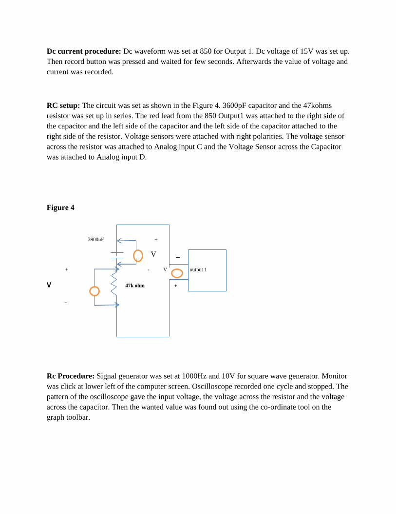
RC setup: The circuit was set as shown in the Figure 4. 3600pF capacitor and the 47kohms

resistor was set up in series. The red lead from the 850 Output1 was attached to the right side of

the capacitor and the left side of the capacitor and the left side of the capacitor attached to the

right side of the resistor. Voltage sensors were attached with right polarities. The voltage sensor

across the resistor was attached to Analog input C and the Voltage Sensor across the Capacitor

was attached to Analog input D.

Figure 4

3900uF +

V _

+ - V output 1 V 47k ohm + _

Rc Procedure: Signal generator was set at 1000Hz and 10V for square wave generator. Monitor

was click at lower left of the computer screen. Oscilloscope recorded one cycle and stopped. The

pattern of the oscilloscope gave the input voltage, the voltage across the resistor and the voltage

across the capacitor. Then the wanted value was found out using the co-ordinate tool on the

graph toolbar.

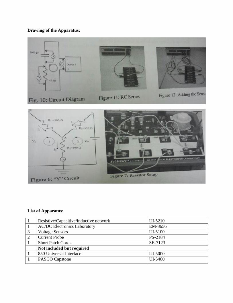
Drawing of the Apparatus:

List of Apparatus:

1 Resistive/Capacitive/inductive network UI-5210

1 AC/DC Electronics Laboratory EM-8656

3 Voltage Sensors UI-5100

2 Current Probe PS-2184

1 Short Patch Cords SE-7123

Not included but required

1 850 Universal Interface UI-5000

1 PASCO Capstone UI-5400

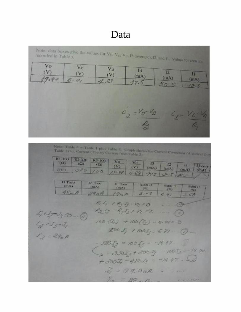
Data

Analysis

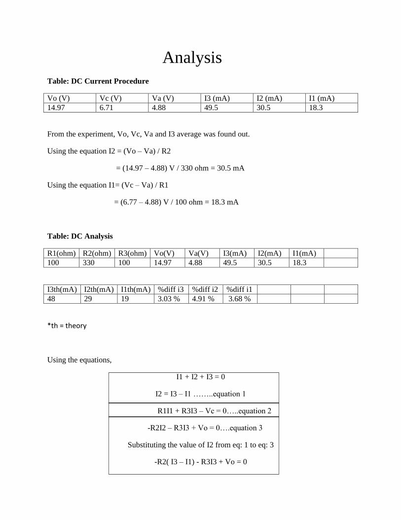
Table: DC Current Procedure

Vo (V) Vc (V) Va (V) I3 (mA) I2 (mA) I1 (mA)

14.97 6.71 4.88 49.5 30.5 18.3

From the experiment, Vo, Vc, Va and I3 average was found out.

Using the equation I2 = (Vo – Va) / R2

= (14.97 – 4.88) V / 330 ohm = 30.5 mA

Using the equation I1= (Vc – Va) / R1

= (6.77 – 4.88) V / 100 ohm = 18.3 mA

Table: DC Analysis

R1(ohm) R2(ohm) R3(ohm) Vo(V) Va(V) I3(mA) I2(mA) I1(mA)

100 330 100 14.97 4.88 49.5 30.5 18.3

I3th(mA) I2th(mA) I1th(mA) %diff i3 %diff i2 %diff i1

48 29 19 3.03 % 4.91 % 3.68 %

*th = theory

Using the equations,

I1 + I2 + I3 = 0

I2 = I3 – I1 ……..equation 1

R1I1 + R3I3 – Vc = 0…..equation 2

-R2I2 – R3I3 + Vo = 0….equation 3

Substituting the value of I2 from eq: 1 to eq: 3

-R2( I3 – I1) - R3I3 + Vo = 0

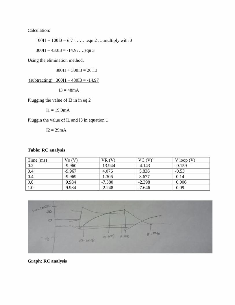
Calculation:

100I1 + 100I3 = 6.71……..eqn 2 ….multiply with 3

300I1 – 430I3 = -14.97….eqn 3

Using the elimination method,

300I1 + 300I3 = 20.13

(subtracting) 300I1 – 430I3 = -14.97

I3 = 48mA

Plugging the value of I3 in in eq 2

I1 = 19.0mA

Pluggin the value of I1 and I3 in equation 1

I2 = 29mA

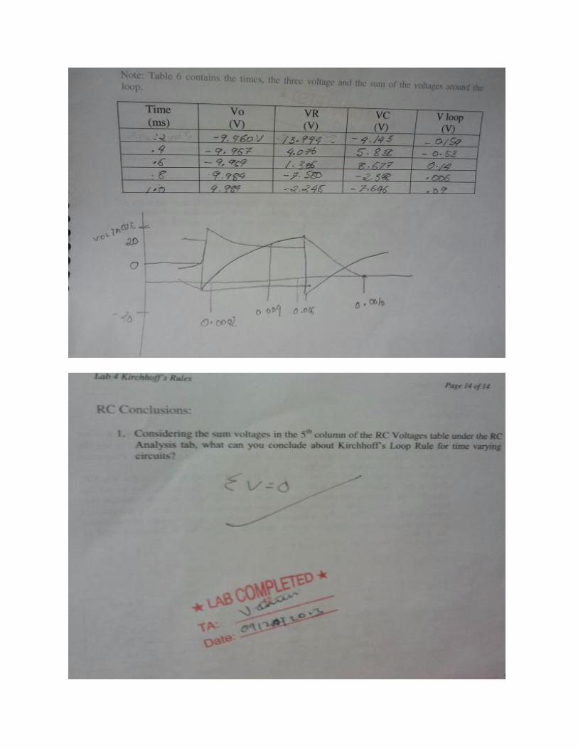
Table: RC analysis

Time (ms) Vo (V) VR (V) VC (V)` V loop (V)

0.2 -9.960 13.944 -4.143 -0.159

0.4 -9.967 4.076 5.836 -0.53

0.4 -9.969 1.306 8.677 0.14

0.8 9.984 -7.580 -2.398 0.006

1.0 9.984 -2.248 -7.646 0.09

Graph: RC analysis

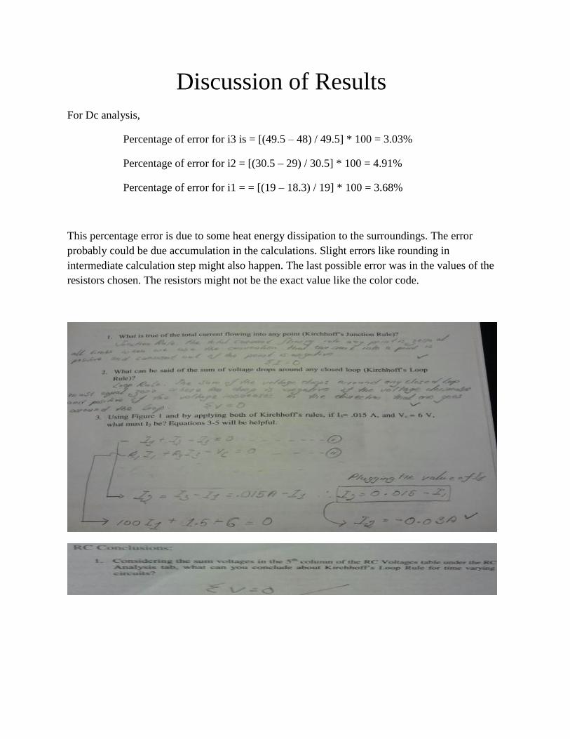
Discussion of Results

For Dc analysis,

Percentage of error for i3 is = [(49.5 – 48) / 49.5] * 100 = 3.03%

Percentage of error for i2 = [(30.5 – 29) / 30.5] * 100 = 4.91%

Percentage of error for i1 = = [(19 – 18.3) / 19] * 100 = 3.68%

This percentage error is due to some heat energy dissipation to the surroundings. The error

probably could be due accumulation in the calculations. Slight errors like rounding in

intermediate calculation step might also happen. The last possible error was in the values of the

resistors chosen. The resistors might not be the exact value like the color code.

Conclusions

The purpose of this lab was to prove the Kirchhoff’s law. Ohm’s law, KVL and KCL are three of

the most basic techniques for the analysis of linear circuits. A circuit was given with unknown

voltages and unknown currents. The voltage and current values were measured and placed into

KVL and KCL equations to determine whether it follows the Kirchhoff’s law or not. The

calculated and measured values of current were compared with theoretical value. The percentage

error was small. Hence the test was considered valid. The errors could be eliminated using

shorter connecting wires. Error could be reduced using by not rounding up the voltage or current

values. The method could be better if we used breadboard to build the circuit. Therefore, the

method we used was precise and accurate.