Experimental Comparison of Bohm-like Theories with Different Primary Ontologies

Arthur O. T. Pang,1, ∗ Hugo Ferretti,1 Noah Lupu-Gladstein,1 Weng-Kian Tham,1 Aharon

Brodutch,1, † Kent Bonsma-Fisher,1, 2, ‡ J. E. Sipe,1, § and Aephraim M. Steinberg1, 3, ¶

1Department of Physics and Centre for Quantum Information Quantum ControlUniversity of Toronto, 60 St George St, Toronto, Ontario, M5S 1A7, Canada

2National Research Council of Canada, 100 Sussex Dr, Ottawa, Ontario, K1A 0R6, Canada3Canadian Institute for Advanced Research, Toronto, Ontario, M5G 1M1, Canada

(Dated: November 19, 2020)

The de Broglie-Bohm theory is a hidden-variable interpretation of quantum mechanics whichinvolves particles moving through space along deterministic trajectories. This theory singles outposition as the primary ontological variable. Mathematically, it is possible to construct a similartheory where particles are moving through momentum-space, and momentum is singled out as theprimary ontological variable. In this paper, we construct the putative particle trajectories for a two-slit experiment in both the position and momentum-space theories by simulating particle dynamicswith coherent light. Using a method for constructing trajectories in the primary and non-primaryspaces, we compare the phase-space dynamics offered by the two theories and show that they donot agree. This contradictory behaviour underscores the difficulty of selecting one picture of realityfrom the infinite number of possibilities offered by Bohm-like theories.

I. INTRODUCTION

Bohm’s hidden-variable interpretation of quantum me-chanics [1, 2], also known as Bohmian mechanics or deBroglie-Bohm theory [3, 4], is an alternative formulationof quantum mechanics with a clear deterministic ontol-ogy, and experimental predictions that match those ofquantum theory. The theory continues to attract atten-tion as a provocative demonstration that a deterministic,no-collapse interpretation of quantum mechanics is pos-sible [5–11]. As is the case in classical physics, Bohmianparticles have well defined properties at all times. InBohmian theory all properties can be determined fromthe particle’s actual position and the guiding wave, givingposition special ontological significance. Wiseman [12]showed that it is possible to experimentally extract thevelocities attributed to Bohmian particles by taking con-ditional averages of weak measurements on an ensembleof post-selected systems. Extending his ideas, some ofthe present authors and others were recently able to con-struct the putative Bohmian trajectories in various two-slit experiments [7, 8, 10, 11].

The choice of position as the primary ontological vari-able introduces an asymmetry which is foreign to bothclassical and quantum mechanics. In classical Hamil-tonian mechanics, position and momentum act as thecanonical phase space variables and are both equally im-portant in formulating the theory, and in orthodox quan-tum mechanics position and momentum are treated onequal footing. So the importance placed on position inthe Bohmian approach was one of the main criticisms of

∗ arthur.pang@mail.utoronto.ca† brodutch@physics.utoronto.ca‡ kent.bonsma-fisher@nrc-cnrc.gc.ca§ sipe@physics.utoronto.ca¶ steinberg@physics.utoronto.ca

Bohm’s work by the pioneers of quantum theory [13].Shortly after Bohm’s paper appeared, Epstein [14, 15]pointed out that there is nothing inherent in the formu-lation that requires position to be the primary ontolog-ical variable, and that other possible choices can leadto other results - i.e. different ontological descriptions -while still yielding experimental predictions identical tothose of quantum theory.

In this paper, we demonstrate how different choices ofthe primary ontological variable can lead to qualitativelydifferent trajectories. Using light in a double-slit setupto simulate the mechanics of massive particles [16], andbuilding on a previously demonstrated approach [7, 8], weconstruct the trajectories in both Bohm’s theory (whichwe refer to as x-Bohm) and an alternative theory in whichmomentum is the primary ontological variable (p-Bohm).The differences between the trajectories in the two the-ories illustrate why the results of previous experiments[7, 8] should be understood as specific instances of themany possible ontological descriptions of the same sys-tem. Selecting one out of the multitude of possible theo-ries – with their conflicting phase-space dynamics of thestate of the system – requires supplementary assumptionsor assertions [5, 12, 17], emphasizing one of the featuresin Bohm’s approach that some would consider a weak-ness.

We begin in Sec. II by describing some of the basicfeatures of the x-Bohm and p-Bohm theories, and themethod for constructing trajectories through a sequenceof weak and strong measurements. In Sec. III we lay outthe details of our experiment, including the specifics ofthe lens system and the weak measurement procedure.The results of the experiments, including plots of thetrajectories and phase space snapshots at the near andfar field are presented in Sec. IV for both the x-Bohmand p-Bohm theories. The implications of our results arediscussed in Sec. V.

arX

iv:1

910.

1340

5v3

[qu

ant-

ph]

17

Nov

202

0

2

II. BOHMIAN THEORY

Contrary to classical mechanics, which allows for thedeterministic prediction of the motion of particles, quan-tum mechanics only offers statistical predictions for theresults of measurements. Yet in 1952 David Bohm in-troduced [1, 2] a deterministic dynamical theory thatits advocates argue provides an underlying descriptionmore fundamental than quantum mechanics [17, 18]. Inhis generalization and extension of earlier ideas by deBroglie [17], the positions of particles play the role ofhidden-variables; their motion is characterized by well-defined trajectories, as the particles are “guided” by theSchrodinger wave. In this approach, position variables,together with the Schrodinger wave, have a special signif-icance as the primary ontological variables; the momentaof particles simply follow from their velocities, which aredetermined by the gradient of the Schrodinger wave atthe positions of the particles. The symmetry of posi-tion and momentum that characterizes orthodox quan-tum mechanics is broken, with position variables morefundamental than momentum variables.

Shortly after Bohm’s work appeared, Epstein [14, 15]noted that different choices of the primary ontologicalvariable can lead to different theories. In particular,one could work with the momentum representation ofthe wave function and build a theory where particlesare characterized fundamentally by their momenta1. Incontrast to Bohm’s original theory, which we refer to as“x-Bohm,” in Epstein’s proposal, which we refer to as a“p-Bohm” theory, it is momentum that has primary onto-logical status. In his reply to Epstein [19], Bohm pointedout technical difficulties in implementing a “p-Bohm” ap-proach when the Hamiltonian involved the Coulomb po-tential. But he also argued that an “x-Bohm” approach,where particle position and the coordinate representationof the wave function are the primary ontological vari-ables, seemed more favored because “in all fields otherthan the quantum theory, space and time have thus farstood out as the natural frame for the description of theprogress of physical phenomena.” [19] Nevertheless, al-ternate approaches were developed further a few decadeslater by Bohm and his collaborators [20], and a gen-eral framework for such theories was discussed by Hol-land [4, 21, 22] and others [23, 24].

In the rest of this section we sketch both x-Bohm andp-Bohm theory, discuss the trajectories that follow fromeach, and show how – under the assumption that one ofthe theories is correct – its associated trajectories can berevealed by weak measurements. We begin with trajec-tories of the primary ontological variable of the particles– position for x-Bohm and momentum for p-Bohm – andthen turn to the trajectories that can be associated with

1 The possibility of a velocity-based theory had already been raisedby Pauli at the 1927 Solvay conference in response to de Broglie’spilot wave theory [1, 17].

non-primary variables. This allows us to compare the twotheories by contrasting their predictions for trajectoriesin the same space. We focus on the one-dimensional mo-tion of a single particle, where the classical Hamiltonianas a function of position and momentum is H(x, p), anddenote the coordinate wave function by ψ(x, t) and the

momentum wave function by ψ(p, t). The Schrodingerequations for these two wave functions are

ih∂

∂tψ(x, t) =H

(x,−ih ∂

∂x

)ψ(x, t) (1)

ih∂

∂tψ(p, t) =H

(ih∂

∂p, p

)ψ(p, t). (2)

A. Position Ontological Bohmian Theory (x-Bohm)

In Bohm’s original theory [1, 2], the particle’s posi-tion and the wave function ψ(x, t) constitute the objec-tively real elements from which all other properties canbe derived2. In describing an ensemble of experimen-tal runs, at some initial time (t = 0) each particle isassumed to have a definite position according to a prob-ability distribution function |ψ(x, 0)|2, and each particleis guided through space by the wave function. Writingψ (x, t) = Rx (x, t) exp [iSx (x, t) /h], where Rx (x, t) andSx (x, t) are real functions of position and time, for aHamiltonian of the form H(x, p) = p2/2m + V (x) theguidance equation is

vx (x, t) =1

2m

∂Sx(x, t)

∂x, (3)

and the trajectory for each particle is given by

dx (t)

dt= vx (x (t) , t) . (4)

Since the expression (3) for the velocity vx(x, t) can alsobe written as [4]

vx (x, t) =jx (x, t)

|ψ (x, t)|2, (5)

where jx(x, t) is the usual probability current density oforthodox quantum mechanics,

jx (x, t) =h

2mi

(ψ∗ (x, t)

∂ψ (x, t)

∂x− ψ (x, t)

∂ψ∗ (x, t)

∂x

),

(6)

2 For an N -particle system the wave function is a function overthe 3N -dimensional configuration space of the system, and sincethe wave function is granted ontological significance that config-uration space must be taken as the underlying arena of reality;the wave function and a point in this configuration space, iden-tifying the positions of all N particles, are best taken to identifythe ontology of the theory.

3

it follows that as the particles in the ensemble move,and as ψ(x, t) evolves according to Schrodinger’s equation(1), the evolution of the distribution function character-izing the positions of the particles follows the evolutionof |ψ(x, t)|2.

Although the Bohmian trajectories had been studiedtheoretically and discussed in the literature since 1952(see, e.g., Philippidis et al. [6]), it seems it was not untilWiseman’s work in 2007 [12] that a strategy for identi-fying them experimentally was investigated. Wisemanpointed out that the expression (3) for the velocity of aparticle at x, which can be written as [4]

vx (x, t) =1

mRe

[〈x| p |ψ (t)〉〈x|ψ (t)〉

], (7)

where p is the momentum operator (〈x|p|x′〉 = −ih∂δ(x−x′)/∂x), can be connected with the theory of weak mea-surements introduced by Aharonov, Albert, and Vaid-man (AAV) [25]. Weak measurements are those withsmall back action and consequently high uncertainty, andWiseman noted that the expression (7) corresponds tothe operational prescription of a weak momentum mea-surement followed immediately by a strong (projective)position measurement. The apparent simultaneous mea-surement of two conjugate variables respects the un-certainty relations since the momentum measurement isweak, and consequently the measurement scenario mustbe repeated many times with the averaging done sepa-rately for every final value of position. This fits neatlyinto the Bohmian perspective in general: Since all vari-ables in the theory are uniquely determined by the pri-mary ontological variable, it could be argued that ensem-ble averaging is justified as long as post-selection ontothe primary ontological value for each experimental runis sufficiently accurate and the measurement back actionfrom the weak measurement is sufficiently small.

Of course, the identification of the right-hand-side of(7) with a weak momentum measurement followed by astrong position measurement can be made operationally,independent of any proposed explanation of quantum me-chanics in terms of a deeper theory. Nonetheless, thetrajectories that are predicted by x-Bohm theory can beformally constructed from the results of weak measure-ments; this has been done by Kocsis et al. [7] for a singleparticle in a double-slit interferometer, and by Mahleret al. [8] for entangled particles. Advocates of x-Bohmtheory then identify these constructed trajectories withtrajectories that are held to really exist.

B. Momentum Ontological Bohmian Theory(p-Bohm)

In p-Bohm theory one adopts momentum as the pri-mary ontological variable, and the fundamental dynamicstake place in momentum-space. Here one relies on themomentum representation of the wave function ψ(p, t),and for Hamiltonians of the form H(x, p) = p2/2m+V (x)

there is no general expression for the time derivativevp(p, t) of the momentum of a Bohmian particle,

dp (t)

dt= vp (p (t) , t) , (8)

which would be analogous to the corresponding expres-sion (3) for the time derivative vx(x, t) of the positionof a Bohmian particle in x-Bohm theory. This can betraced to the fact that all such Hamiltonians exhibit thesame dependence on p but, depending on the potential,can have very different dependences on x; thus, whileSchrodinger’s equation in configuration space (1) involvesonly second derivatives with respect to x, Schrodinger’sequation in momentum-space (2) can involve any num-ber of derivatives with respect to p. Nonetheless, onecan look for an expression for vp(p, t) analogous to theexpression (5) for vx(x, t), writing

vp(p, t) =jp(p, t)∣∣∣ψ(p, t)

∣∣∣2 , (9)

where jp(p, t) is a current density in momentum-space.In a one-dimensional problem it must satisfy

∂jp(p, t)

∂p= − ∂

∂t

(∣∣∣ψ(p, t)∣∣∣2) , (10)

and since the right-hand-side is determined by theSchrodinger equation in momentum-space (2), a uniquejp(p, t) can be identified,

jp(p, t) =2

h

∫ p

−∞Im

(ψ∗(p′, t)

(V (ih

∂

∂p′)ψ(p′, t)

))dp′,

(11)

under the physically reasonable assumption thatjp(p, t) → 0 as |p| → ∞ [23]. The situation is morecomplicated in higher dimensions; in three dimensions,for example, the continuity equation for a momentumcurrent density jp(p, t) only restricts the divergence ofjp(p, t) and not its curl, and it is not immediately clearhow it should be assigned. The range of possible choicesfor current densities in general de Broglie-Bohm theo-ries, and the criteria one might want to apply in makinga choice, have been investigated by Struyve and Valen-tini [23]. Our focus in this paper will be on free particles

(V (x) = 0), where the distribution∣∣∣ψ(p, t)

∣∣∣2 of Bohmian

particles in momentum-space is time independent, andfrom (9,11), and in agreement with physical intuition,we have vp(p, t) = 0.

C. Trajectories in a non-primary space

Although a Bohmian theory is deterministic, with awell-defined evolution of dynamical variables once the ini-tial conditions are specified, the phase space description

4

of dynamics so useful in classical theories is at first sightnot a natural one here. A Bohmian theory always iden-tifies a primary ontological variable, which in x-Bohmtheory is particle position. Of course, in this theory onecan multiply the velocity of the Bohmian particle – whichis determined once the wave function and the particle po-sition are specified – by the mass of the particle and soidentify a particle momentum. But it has a diminishedstatus in x-Bohm theory compared to its role in classi-cal dynamics, for the initial momentum of the particlecannot be specified independently of the initial positionof the particle. The proper arena of dynamics seems tobe configuration space, in which the particle position is apoint and over which the wave function is defined, ratherthan phase space.

The situation is more drastic for p-Bohm theory, es-pecially in the case of a classically free particle thatwe consider here. Momentum is the primary ontologi-cal variable, the proper arena of dynamics is clearly thespace associated with momentum, and for a free particlethe momentum of the Bohmian particle does not change.The non-primary variable of particle position does noteven seem to arise, and in this theory one can even won-der whether or not the question of what each particleis doing in configuration space is meaningful. Thus inboth the x-Bohm and p-Bohm theories the significanceof phase-space is unclear without proper treatment of thenon-primary variables.

In his consideration of the status of variables inBohmian theories, Holland [4, 21] suggested a strategyfor identifying the values of variables other than the pri-mary ontological variable, thus allowing in general for avisualization of the underlying dynamics in phase space.For one-dimensional systems and in our notation, if weconsider a “ξ-Bohm theory,” where here ξ is an eigen-

value of a Hermitian operator ξ that we take to havecontinuous eigenvalues, the value ω of a continuous vari-able associated with a Hermitian operator ω is taken tobe

ωξ(ξ, t) = Re

[〈ξ| ω |ψ (t)〉〈ξ|ψ (t)〉

](12)

at time t, if the ket is |ψ(t)〉 and the primary ontologicalvariable has value ξ. Holland did not take this suggestionto be at the level of a new postulate, and even consideredother approaches for some physical systems. Nonetheless,the proposal has the physically comforting feature thatthe average of the values granted to a variable ω over anensemble of Bohmian particles described by a ξ-Bohmtheory does agree with the expectation value of the op-erator associated with that variable in the ket describingthe ensemble,

〈ψ(t)|ω|ψ(t)〉 =

∫ωξ(ξ, t) |〈ξ|ψ(t)〉|2 dξ. (13)

As an example, consider momentum in an x-Bohm the-ory. For a particle at position x at time t, from (12) we

see that the value of momentum that would be assignedis

px(x, t) = Re

[〈x| p |ψ (t)〉〈x|ψ (t)〉

]. (14)

Comparing with the x-Bohm expression (7) for vx(x, t),we find

px(x, t) = mvx(x, t), (15)

as would be physically expected. Yet we can now also as-sign evolving position variables to particles in a p-Bohmtheory, for the prescription (12) gives

xp(p, t) = Re

[〈p| x |ψ (t)〉〈p|ψ (t)〉

], (16)

and following xp(p, t) as t advances allows us to assign atrajectory in real space to a Bohmian particle in p-Bohmtheory with momentum p.

Remarkably, Holland’s prescription (12) is preciselythat which operationally characterizes a weak ω mea-

surement followed by a strong ξ measurement. Thus,just as velocities of particles in an x-Bohm theory canbe constructed by weak momentum measurements fol-lowed by strong position measurements, so the positionsof particles in a p-Bohm theory can be constructed byweak position measurements followed by strong momen-tum measurements. And so we have a route to identi-fying trajectories of Bohmian particles in “non-primary”spaces, by which we mean spaces associated with vari-ables other than the primary ontological variable. Thisis done by first constructing the trajectories of the pri-mary ontological variable, leading to an equation for ξ(t)and then using Eq. (12) to construct the trajectory givenby ω(ξ(t), t). We can experimentally construct trajecto-ries in momentum-space for particles in an x-Bohm the-ory, as indeed has already been done implicitly in [7, 8]and explicitly in [11], both relying on (15). Addition-ally, we can also experimentally construct trajectories inposition-space for particles in a p-Bohm theory. We willuse these trajectories as basis to compare the phase-spacedynamics of different Bohm-like theories, and will turnto this in the following sections.

III. EXPERIMENTAL SCHEME

In our experiment, we simulate the evolution of a mas-sive particle under x-Bohm and p-Bohm theories withlight from a laser diode, using the fact that light propa-gating in the paraxial regime can be modelled with theSchrodinger equation. The propagation of monochro-matic light can be modelled with the Helmholtz equation[26]

∇2U + |k|2U = 0, (17)

5

where U is a complex amplitude and k = (kx, ky, kz) isthe wave vector. In the paraxial regime where |k|≈ kz,this equation can be reduced to

i∂

∂zu =

−1

2|k|∂2

∂x2u, (18)

where U = u ·exp (ikzz), u is the envelope function of thepropagating light, z is the longitudinal position, and they coordinate is factored out through a separation of vari-ables. Equation (18) has the form of the one-dimensionalSchrodinger equation (1) for a free particle. Defining aneffective mass through |k|= mc/h, the correspondence ofvariables between optical and massive particle regimes issummarized in Table I. Note that we use the transverseangle θ = kx/|k|, equivalent to a normalized momentum,when plotting results.

Paraxial Light Particle in 1D[plotted units] normalized units

Transverse position: x [mm] Position: xLongitudinal position: z [m] Time: tc

Transverse angle: θ = kx

|k| [rad] Momentum: pmc

TABLE I. Variable correspondence between paraxial light anda particle in 1D. Note that in the derivations we use kx and|k| while the normalized momentum θ is used in the plots.

Drawing the analogy between Eq. (18) and theSchrodinger equation, we simulate the trajectories of par-ticles in a double-slit experiment by sending 915 nm laserlight through a double-slit apparatus, employing the ex-perimental setup outlined in Figures 1 and 2. In the restof this section we describe the details of this setup, be-ginning with the gadget used for the weak momentummeasurement and the procedure employed in the exper-imental construction of position trajectories in x-Bohm,which closely follow those outlined earlier [7, 8]. We thendescribe how the same procedure is used to constructmomentum trajectories in x-Bohm theory, and how thesetup is modified for constructing position trajectories inp-Bohm theory.

A. Weak momentum measurements

A weak measurement is performed by coupling the de-sired observable to a pointer variable, often a different de-gree of freedom of the same physical system, followed bya strong pointer variable measurement [27, 28]. Here weuse polarization as the pointer. Our observable of interestis momentum, which maps to kx for the light beam. We

use kx to denote the operator form of kx. Specifically, in

the position representation 〈x| kx |x′〉 = −i∂δ(x−x′)/∂x.As described below, the shift in polarization will be pro-portional to the weak value which can then be extractedthrough a standard polarization measurement. We usethe notation |H〉, |V 〉 for horizontal and vertical polar-

ization respectively, |D〉 = (|H〉+ |V 〉)/√

2, |A〉 = (|H〉−

X P

Slit setup System of lenses Imaging setup

X P

Beamcoupler

Translationstage

QWP/HWP/Polarizer

Lenses

Beamsplitter

Mirror

Calcitepositionx-Bohm/p-Bohm

Beamdisplacer

Camera

FIG. 1. Illustration of experimental setup in three parts. Theslit setup is used to initialize the double-slit experiment. Adiagonally-polarized beam is split into two co-propagatingbeams using a displaced Sagnac interferometer, where thebeam separation (set to 2 mm throughout the experiment)can be tuned by translating one of the mirrors. The systemof lenses is used to simulate propagation of the light along zover a large range (see Fig. 7 and Fig. 8 for further details).The two plots above the lens system indicate the intensityprofiles of the beam before and after the lens transformation.A thin piece of calcite is used to weakly couple momentumto polarization (the weak measurement). The calcite is po-sitioned before the lenses for the weak momentum measure-ment in the x-Bohm experiment and between the lenses forweak position measurement in the p-Bohm experiment. Theimaging setup, consisting of a polarizing beam displacer anda CCD camera, is used to obtain two interference patterns,one for each polarization.

|V 〉)/√

2 for diagonal and anti-diagonal respectively, and

|R〉 = (|H〉+ i |V 〉)/√

2, |L〉 = (|H〉− i |V 〉)/√

2 for right-and left-circular polarizations, respectively. The pointeris initially set to the diagonal polarization, |D〉. Polar-ization is coupled to the transverse momentum of thelight using a thin calcite crystal. The interaction can bedescribed by the Hamiltonian

HI = hgkx|k|σz (19)

where

σz =1

2(|H〉 〈H| − |V 〉 〈V |) =

1

2(|D〉 〈A|+ |A〉 〈D|) ,

(20)and g is the coupling strength. If the joint state of thetransverse position and polarization before the calcite is|Ψ〉 = |ψ〉⊗|D〉, then with a sufficiently weak interaction,i.e., sufficiently small ζkx = gtkx � 1 over a range ofinterest for kx, the joint state after the calcite is

|Ψ′〉 ≈ |ψ〉 ⊗ |D〉 − i ζ2

kx|k||ψ〉 ⊗ |A〉 . (21)

The interaction is followed by a projective x measure-ment, post-selected on the result, xf . The state of the

6

CalciteLens 2

Focal planeTranslatable

Element QWP Lens 3ImagingSetupLens 2Lens 1

55cm

f2 f3f2+f3+d

∞0m 1m

x-Bohm

Lens 3Focal plane

40cm

f2+f3f2 f3 d∞0m 1m

p-Bohm

FIG. 2. Illustration of the system of lenses configured tomake measurements for x-Bohm (top) and p-Bohm (bottom)theories. The focal lengths of the lenses are f1 = 15 cm andf2 = f3 = 10 cm from left to right, and the total length, fromLens 1 to the imaging setup, is 55 cm. Lens 1 focuses thebeam and remaps the position variable of planes from 0 m toinfinity onto the position variable of planes from 0 cm to 15 cmafter the lens, with a scaling factor. The grey axis indicatesthe correspondence between the location of the focus of Lens2 and the effective propagation distance being imaged by thelens setup. A detailed plot of the propagation distance vs thedisplacement d of Lens 2 is plotted in Figure 7. Top: Lens2 and Lens 3 map the position variable at the dotted line tothe imaging setup (solid line); Bottom: Lens 2 and Lens 3 areset to be 20 cm away from each other, forming a one-to-onetelescope.

pointer following this post-selection is

〈xf |Ψ′〉 ≈ ψ(xf )(e−i

ζ2|k| 〈kx〉w |H〉+ ei

ζ2|k| 〈kx〉w |V 〉

),

(22)where ⟨

kx

⟩w

=〈xf | kx |ψ〉〈xf |ψ〉

(23)

is the weak value, in general a complex number. The realpart of the weak value shows up as a phase shift betweenthe H and V polarizations and can be extracted by theprojective measurement σy = 1

2 (|R〉 〈R| − |L〉 〈L|). Thiscorresponds to making measurements of the right- andleft-circular intensities, resulting in

〈σy〉 = sin

(ζ

|k|Re(⟨kx

⟩w

)). (24)

B. Position trajectories in x-Bohm theory

The double-slit pattern is generated by separating aGaussian beam (1/e2 diameter of 0.55 mm) into two, us-ing a horizontally-displaced Sagnac interferometer (slit

setup in Figure 1), which gives an effective slit separa-tion of 2 mm. The light is then diagonally polarized andsent through a thin calcite crystal (0.2 mm, cut at 45 de-grees) to weakly couple the transverse momentum of thelight to polarization via a birefringent phase shift (seeSec. III A above). Importantly, the interaction Hamilto-nian (19) commutes with the Hamiltonian for free prop-agation. This implies that the calcite crystal can remainfixed at a single z position before the lens system inde-pendent of the plane of interest.

Next, the co-propagating beams traverse a system ofthree lenses (Fig. 1, middle pane), labelled Lens 1, 2,3 with respective focal lengths 15 cm, 10 cm, 10 cm (seeFigure 2). By translating Lens 2 along the z-axis, wesimulate different propagation distances for the light, re-sulting in effective distances ranging from 0.66 m to 3.5 m.In other words, the three-lens system maps what wouldhave been the transverse position of the light beam prop-agating in free space onto the transverse position at theend of the lens system3. The calibration of the lens sys-tem is discussed in Appendix B.

Finally, the co-propagating beams enter the imagingsetup (Fig. 1, right pane), where the resulting intensitypatterns at the end of the lens system were measured ona CCD camera. In addition to the intensity of the inter-ference pattern, the polarization is measured by a quar-ter wave plate and a polarization beam displacer thateffectively separates the left- and right-circularly polar-ized light in the vertical direction. Since the interferenceoccurs along the horizontal transverse axis4, the interfer-ence patterns for the left- and right-circular polarizationscan be measured independently. The intensity patternsof the two polarizations (|u|2 in Eq. (18)), given by IRand IL, differ by an amount directly related to the realpart of the weak value of transverse momentum, whichin the limit of an infinitely weak measurement can beextracted as

Re(⟨kx

⟩w

)|k|

=1

ζ

[sin−1

(IR − ILIR + IL

)− φ0

], (25)

where the sin−1 term comes from Eq. (24) and φ0 is amomentum-independent phase shift acquired in the cal-cite crystal, set by tilting the calcite; ζ = 134.49±0.13 isthe coupling strength5 which depends on the length of thecalcite. The calibration of ζ is discussed in Appendix B.Examples of measured intensity patterns for near- andfar-field propagation distances are shown in the top row

3 With our experimental parameters, λ = 915 nm, slit separations = 2 mm, and slit width w = 0.55 mm, we expect the near-to-farfield transition to occur at s

2/(λ/(πw/2)) = 0.77 m.

4 This is the axis that is horizontal and perpendicular to the axisof propagation.

5 The quantity ζ corresponds to rotation imparted to the polar-ization of light per transverse angle of the light, and is hencedimensionless.

7

of Figure 3, while measured values of the momentum, inthe same two planes, are shown in the third row of Fig-ure 3. By performing this measurement for each z-plane,we extracted ensemble-average values of the transversemomentum as a function of position, from which we con-struct particle trajectories. Experimentally constructedx-Bohm position trajectories are shown in the top row ofFigure 4, with theoretically calculated trajectories shownin the bottom row. We will discuss all experimental re-sults in greater detail in Section IV.

C. Momentum trajectories in x-Bohm theory

To construct the momentum trajectories in x-Bohm wefollow the procedure outlined in Sec. II C, where again weuse Eq. (14). In our case the momentum is proportionalto the velocity (see Eq. (15)), which implies that themeasurement performed to construct the x trajectoriesin Section III B suffices for constructing the momentumtrajectories. The resulting trajectories are shown in thefirst row of Figure 5.

Note that proportionality between velocity and mo-mentum is only valid when the potential term in theHamiltonian is independent of p. In cases where the po-tential has p and/or p2 terms, Eq. (7) is no longer valid,while Eq. (14) remains valid generically.

D. Momentum trajectories in p-Bohm theory

As described in Sec. II B, the conservation of momen-tum for a free particle implies that the p-Bohm momen-tum trajectories follow lines of constant p. There is noneed to construct these trajectories experimentally; how-ever, the relative probabilities (or density of trajectories)can be measured by making a strong p measurement. Inpractice this is accomplished by strong x measurementsin the far field, using the fact that momentum maps toposition at infinity (see Figure 8 in Appendix B). Thesame setup is used to calibrate the coupling strength ofthe weak measurement (again, see Appendix B). The re-sulting trajectories are shown in the second row of Fig-ure 5.

We emphasize that p-Bohm theory in three dimensionsis not unique, and that different theories lead to differ-ent expressions vp(p, t) for the momentum-space velocity[23]. However, in one dimension the continuity constraint(10) essentially identifies (11) as the current density inmomentum-space, which in the limit of a free particleleads via Eq. (9) to the conservation of the p-Bohm mo-mentum. The results in Fig. 5 are therefore free of anyambiguity that would affect p-Bohm theories in higherdimensions.

E. Position trajectories in p-Bohm theory

Position is a non-primary variable in p-Bohm theory,with the procedure of constructing its trajectory givenin Sec. II C using Eq. (16). This amounts to makingweak position measurements followed by a post-selectionon momentum. To perform the weak measurement, Lens2 and Lens 3 are kept at a fixed distance from one an-other, making a one-to-one telescope, and are translatedtogether (Figure 2). In this way, the transverse momen-tum between Lens 2 and Lens 3 corresponds to transverseposition in a fixed propagation plane. As such, the cal-cite crystal is placed in between Lens 2 and Lens 3 toperform a weak position measurement. Additionally, theone-to-one telescope relates the light one focal length be-fore Lens 2 to the light one focal length after Lens 3 byan identity transformation. This effectively places thefar field of the interfering beams onto the imaging setup,causing it to perform a strong momentum measurement.To read out the weak measurement, the quarter waveplate and polarization beam displacer, once again, areused to separate the left- and right-circularly polarizedcomponent of the beam in the vertical direction and, withprocedures similar to those in Section III B, we can ex-tract the weak position value post-selected on momen-tum. The fourth row of Figure 3 shows results of thecorresponding weak measurements in near- and far-fieldplanes. Position trajectories, with momentum as the pri-mary ontological variable, are constructed in the samemanner as before. Constructed trajectories are shown inthe second row of Figure 4.

IV. COMPARISON OF x-BOHM AND p-BOHMTRAJECTORIES

We now consider the x-Bohm and p-Bohm particle tra-jectories in detail. The trajectories are constructed byinterpolating data points taken at discrete z-planes rang-ing from an effective distance of 0.66 m to 3.5 m after theslits. The results presented and discussed below showthe qualitatively different behavior of the trajectories inthe two theories, especially in the near-field. The experi-mental results are in good agreement with the theoreticalpredictions, and illustrate the dependence of the ontolog-ical description on the choice of the primary ontologicalvariable.

A. Single-time position-momentum snapshots

For a given z-plane, which corresponds to an instantin time, data were taken by fixing the lenses and post-selecting on the primary ontological variable producing acomplete description of the functions p (x, t) and x (p, t)for the x-Bohm and p-Bohm theories respectively. Re-sults for two of these instants of time, one in the near-field and one in far-field, are presented in Figure 3 and

8

-3 -2 -1 0 1 2 3

Position (mm)

-2

-1

0

1

2

Mom

entu

m (

mra

d)

Weak values theoretical, near field

-5 0 5

Position (mm)

-2

-1

0

1

2

Mom

entu

m (

mra

d)

Weak values theoretical, far field

-3 -2 -1 0 1 2 3

Position (mm)

0

0.5

1

Inte

nsity

(ar

b. u

nits

)

Intensity distribution experimental, near field

-5 0 5

Position (mm)

0

1

2

3

4

Inte

nsity

(ar

b. u

nits

)

Intensity distribution experimental, far field

-3 -2 -1 0 1 2 3

Position (mm)

-2

-1

0

1

2

Mom

entu

m (

mra

d)

x-Bohm experimental result, near field

-3 -2 -1 0 1 2 3

Position (mm)

-2

-1

0

1

2

Mom

entu

m (

mra

d)

p-Bohm experimental result, near field

-5 0 5

Position (mm)

-2

-1

0

1

2M

omen

tum

(m

rad)

x-Bohm experimental result, far field

-5 0 5

Position (mm)

-2

-1

0

1

2

Mom

entu

m (

mra

d)

p-Bohm experimental result, far field

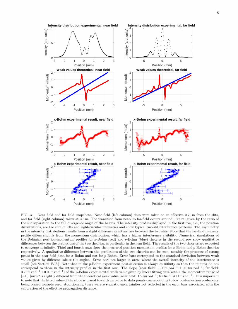
FIG. 3. Near field and far field snapshots. Near field (left column) data were taken at an effective 0.70 m from the slits,and far field (right column) taken at 3.5 m. The transition from near- to far-field occurs around 0.77 m, given by the ratio ofthe slit separation to the full divergence angle of the beams. The intensity profiles displayed in the first row, i.e., the positiondistributions, are the sum of left- and right-circular intensities and show typical two-slit interference patterns. The asymmetryin the intensity distributions results from a slight difference in intensities between the two slits. Note that the far-field intensityprofile differs slightly from the momentum distribution, which has a higher interference visibility. Numerical simulations ofthe Bohmian position-momentum profiles for x-Bohm (red) and p-Bohm (blue) theories in the second row show qualitativedifferences between the predictions of the two theories, in particular in the near field. The results of the two theories are expectedto converge at infinity. Third and fourth rows show the measured position-momentum profiles for x-Bohm and p-Bohm theoriesrespectively. A qualitative difference between the predictions of the two theories can be seen, notably the presence of strongpeaks in the near-field data for x-Bohm and not for p-Bohm. Error bars correspond to the standard deviation between weakvalues given by different calcite tilt angles. Error bars are larger in areas where the overall intensity of the interference issmall (see Section IV A). Note that in the p-Bohm experiment post-selection is always at infinity so that the minima do notcorrespond to those in the intensity profiles in the first row. The slope (near field: 1.03m rad−1 ± 0.01m rad−1; far field:3.70mrad−1±0.09mrad−1) of the p-Bohm experimental weak value given by linear fitting data within the momentum range of[−1, 1]mrad is slightly different from the theoretical weak value (near field: 1.21mrad−1; far field: 4.11mrad−1). It is importantto note that the fitted value of the slope is biased towards zero due to data points corresponding to low post-selection probabilitybeing biased towards zero. Additionally, there were systematic uncertainties not reflected in the error bars associated with thecalibration of the effective propagation distance.

9

compared with theoretical predictions. To illustrate thedifference between the two theories we begin with a nu-merically simulated plot (Figure 3, second row), where weoverlay two ontological momentum-position snapshots,based on Eq. (12). Experimental results are shown inthe third and fourth rows of Figure 3.

In x-Bohm, peaks in the momentum p (x, t) appearwhen a particle approaches a minima in the double-slitinterference pattern (i.e. the minima in the top row ofFigure 3). These peaks get progressively narrower, withwidth approaching zero, as the measurement is taken fur-ther into the far field. The asymptotic large x behaviorof the function p (x) corresponds to

p/m =x− sgn(x)w/2

t, (26)

with t being propagation time and w = 2 mm being theslit separation. This can be roughly interpreted as theconsequence of the guiding wave ψ(x, t) at the near fieldhaving two distinguishable parts with a small overlap sothat particles away from the overlap are effectively guidedby one or the other, leading to behaviour similar to whatone would observe if only one slit were open.

In p-Bohm theory, we expect a linear relation x (p) =p ·t/m. It is important to note that, experimentally, datawith momentum post-selection always projects the farfield onto the imaging setup. Similarly, the guiding waveψ(p, t) has the form of the far-field interference pattern.

Due to the nature of our measurement, the weak valueof the variable of interest is very sensitive to backgroundnoise when the post-selection probability is small. Whenbackground light and other systematic errors dominatethe measured signal, the probability of registering a mea-surement in the left- and right-circular polarization basisbecomes roughly equal. As a consequence, and by refer-ring to Eq. (25), one can see that the weak value tendsto the incorrect result of −ζ−1φ0 near the minima of theinterference patterns. As mentioned in Section III B, thevalue of φ0 in our experiment is controlled by the hor-izontal tilt angle of the calcite crystal. In an idealizednoiseless measurement, the value of φ0 exists purely as acalibration parameter of the weak measurement (see Ap-pendix B) and does not affect the measured weak value.However, with some amount of noise present in the mea-surements this is not the case. To account for this im-perfection, we measured weak values using various calcitetilts. The final weak value at each time is tabulated byaveraging measurement results with different calcite tilts.Error bars in the third and fourth row of Figure 3 cor-respond to the standard deviation of the measurementgiven a set of values for φ0. The effects of the calcitetilt are particularly pronounced in p-Bohm experiments,where the measurements at the minima go very close tozero and the standard deviation between measurementresults increases significantly.

B. Constructing Trajectories

We construct a set of trajectories for both position andmomentum in both x-Bohm and p-Bohm theory, chosenso that the density of the selected trajectories in the pri-mary ontological space corresponds to particle distribu-tion probabilities. This is possible due to the fact thatthe velocities are defined through the probability current(see Sec. II). However, there is no a priori reason toexpect this feature to be preserved in the non-primaryspace, and indeed we will see that it is not. Similarly,the trajectories in the primary space cannot cross, sincegiven a wave function, the velocity is uniquely defined bythe value of the primary ontological variable. As we willsee, the p(x, t) trajectories in x-Bohm do cross. The tra-jectories for x-Bohm and p-Bohm experiments are shownin Figures 4 and 5 respectively along with theoreticaltrajectories derived from a numerical simulation.

1. Position Trajectories

The x-Bohm position trajectories shown in the top rowof Figure 4 are very similar in nature to those obtainedearlier [7]. These trajectories originate from one of thetwo slits and, while providing the signatures of interfer-ence for the probability density, they generally divergeaway from x = 0 while displaying a rapid ‘acceleration’through each region of destructive interference, where thedensity becomes low and the ratio of flux to density cor-respondingly large. As required by the Bohmian formal-ism, the trajectories of the primary ontological variabledo not cross.

For p-Bohm, the position trajectories (Figure 4 mid-dle) originate from a single point in between the two slitsand spread out in a manner that preserves momentum,resulting in straight lines given by x = pt/m. A crossing(or in this case convergence to a point at t = 0) is pos-sible since these are not the trajectories of the primaryontological variable. Imperfect translation of Lens 2 andLens 3 causes some transverse displacement, leading toa systematic error in the weak value measurement suchthat the trajectories are displaced by a different amountat each plane. This causes the trajectories to shift in they-axis of Figure 4, resulting in the experimental weakvalues of position deviating from simple straight lines.

Apart from the obvious discrepancy between the posi-tion trajectories in x-Bohm and p-Bohm, the p-Bohm po-sition trajectories exhibit the potentially surprising phe-nomenon of originating at x = 0, rather than in eitherof the slits. That is, the initial position for all the parti-cles according to p-Bohm theory is a position which hasvanishingly low probability according to x-Bohm; more-over, a detector placed at that position would never beexpected to register a photon. Note that since the valueof position in p-Bohm is given by the weak value (14),it is different from the result of the projective positionmeasurement that is associated with the double slit or a

10

0.5 1 1.5 2 2.5 3 3.5

Propagation distance (m)

-4

-2

0

2

4

Tra

nsve

rse

disp

lace

men

t (m

m)

Experimental p-Bohm position trajectories

0.5 1 1.5 2 2.5 3 3.5

Propagation distance (m)

-4

-2

0

2

4T

rans

vers

e di

spla

cem

ent (

mm

)

Experimental x-Bohm position trajectories

0.5 1 1.5 2 2.5 3 3.5

Propagation distance (m)

-4

-2

0

2

4

Tra

nsve

rse

disp

lace

men

t (m

m)

Theoretical x-Bohm and p-Bohm position trajectories

FIG. 4. Constructed position trajectories based on x-Bohm (red) and p-Bohm (blue) theories. Top (middle) plot corresponds tox-Bohm (p-Bohm) position trajectories constructed experimentally. Bottom plot corresponds to numerical simulation of bothx-Bohm (red solid line) and p-Bohm (blue dotted line) position trajectories overlaid. x-Bohm trajectories originate from thelocation of the two slits, while p-Bohm trajectories originate from mid-point between the two slits. In the far field, trajectoriesfrom x-Bohm and p-Bohm theory converge to the same values as expected. The x-Bohm trajectories are also plotted in Figure6 (top) with one position trajectory highlighted.

11

0.5 1 1.5 2 2.5 3 3.5

Propagation distance (m)

-2

-1

0

1

2

Tra

nsve

rse

mom

entu

m (

mra

d)

Experimental p-Bohm momentum trajectories

0.5 1 1.5 2 2.5 3 3.5

Propagation distance (m)

-2

-1

0

1

2

Tra

nsve

rse

mom

entu

m (

mra

d)

Experimental x-Bohm momentum trajectories

0.5 1 1.5 2 2.5 3 3.5

Propagation distance (m)

-2

-1

0

1

2

Tra

nsve

rse

mom

entu

m (

mra

d)

Theoretical x-Bohm and p-Bohm momentum trajectories

FIG. 5. Constructed momentum trajectories based on x-Bohm (red) and p-Bohm (blue) theories. Top(middle) plot correspondsto x-Bohm(p-Bohm) momentum trajectories constructed experimentally. Bottom plot corresponds to numerical simulationof both x-Bohm (red solid line) and p-Bohm (blue solid line) momentum trajectories overlaid. In the far fields both sets oftrajectories bunch in the manner reflective of the far field interference pattern. The transverse momentum along the momentumtrajectories for x-Bohm are equal to the first derivative of the position along the position trajectories under x-Bohm, whereasthe momentum trajectories for p-Bohm are flat lines due to the conservation of momentum. Peaks in the x-Bohm trajectoriescorresponds to the crossing of the particle over an interference minimum, and their time of occurrence is highly sensitiveto the initial conditions of the primary ontological variable, causing inconsistencies between the numerically simulated andexperimentally constructed trajectories. The design of our experiment presumes conservation of momentum. As a result, themomentum trajectories given by p-Bohm cannot be anything other than flat, reflecting momentum conservation as a built inassumption in our experiment. The x-Bohm trajectories are also plotted in Figure 6 (bottom) with one momentum trajectoryhighlighted.

12

0.5 1 1.5 2 2.5 3 3.5

Propagation distance (m)

-1

-0.5

0

0.5

1T

rans

vers

e di

spla

cem

ent (

mm

)Experimental x-Bohm position trajectories, highlighted

0.5 1 1.5 2 2.5 3 3.5

Propagation distance (m)

-2

-1

0

1

2

Tra

nsve

rse

mom

entu

m (

mra

d) Experimental x-Bohm momentum trajectories, highlighted

FIG. 6. x-Bohm experimental trajectories for position (top)and momentum (bottom) with a single initial setting high-lighted for clarity. Note that the highlighted, non-primaryvariable, trajectory of momentum (bottom) corresponds tothe highlighted ontological trajectory of position (top). Peaksin the momentum trajectories correspond to the ontologicalposition trajectories crossing a minimum in the two-slit inter-ference pattern.

detector. In general, the values of non-primary variablesdo not need to agree with the results of projective mea-surements in standard quantum theory. Indeed in thep-Bohm picture, the initial state prepared in our experi-ment sets the position variable to be zero.

2. Momentum Trajectories

Next, we construct particle momentum trajectories,tracking the change of momentum over time (see Fig-ure 5). As the conservation of momentum of light infree space is an assumption used in the alignment, thep-Bohm momentum trajectories are constructed fromtheory as flat lines with a distribution derived fromthe strong momentum measurement (position in the farfield).

The x-Bohm momentum trajectory functions are pro-portional to the time derivative of the position trajec-tory functions. The peaks observed in x-Bohm momen-tum trajectories correspond to time intervals when theposition trajectories are crossing the minima of the in-terference pattern (as emphasised in Fig. 6). The timeinstances at which these peaks appear are highly sensi-tive to the initial conditions of the x-Bohm position tra-jectories, and as such, they do not align with the peakpositions in the numerical simulation. These peaks indi-cate the non-conservation of momentum in x-Bohm forindividual particle trajectories, which is analogous to theissue of p-Bohm position trajectories originating in be-

tween the two slits discussed in section IV B 1.To further explain the behaviour at the peaks, we high-

light a single trajectory line in Figure 6, where the topand bottom plots correspond to a position and momen-tum trajectory in x-Bohm for the same initial conditions.A peak in the momentum trajectory directly correspondsto the portion of the position trajectory where the par-ticle crosses a minimum in the double-slit interferencepattern.

V. DISCUSSION

When everyone is somebody, then noone’s anybody.W.S. Gilbert, The Gondoliers

The lack of an ontological interpretation has been crit-icised as a serious drawback of quantum theory sinceits early days [17]. Part of the deeper understandingthat an ontological interpretation would provide wouldbe a visualization of the underlying quantum dynamics.Apart from any philosophical considerations, such visu-alizations are arguably essential for developing the intu-ition necessary for scientific development. At the sametime, incorrect visualizations (such as those involving theaether in electrodynamics) can lead us astray. Bohm’s in-terpretation, with its deterministic particle trajectories,presents an attractive visual picture of quantum dynam-ics at the cost of some non-trivial assumptions. Amongthese is an assumption of the role of position and the co-ordinate representation of the wave function as the funda-mental variables that determine the dynamics. Indeed,in contrast to classical physics, where both the initialposition and momentum are necessary for predicting thedynamics that follows, in an x-Bohm theory the initialconditions are just the initial position of the particle,together with the initial wave function. It is thereforetempting to view the identification of the asymmetry asa profound discovery, suggesting that position is indeedmore important than other variables. One could evenhope that the realization that position plays a specialrole would lead to new experimental predictions. How-ever, as emphasized in this work, the specific choice ofposition is not unique, leaving us with an infinite numberof possible primary ontological variables – each allegedlymore fundamental than all the others – or, as Gilbert’sline above implies, with none.

Our main results show that a variation of Bohm’s the-ory (p-Bohm), one in which the primary ontological vari-able is momentum, leads to very different phase-spacedynamics. In this theory the fundamental trajectoriesare paths through momentum-space, and the equationsof motion take a form which is closer to that of New-ton’s laws, with a first time-derivative for momentum.If the underlying phase-space dynamics of both theorieswere the same, one might say that the symmetry between

13

position and momentum had been restored, removing anon-trivial assumption from Bohm’s theory. The picturesare, however, very different (see Figures 3, 4 and 5) andso, the asymmetry in a Bohm-like theory is confirmed butambiguous. One is left to wonder which of the two the-ories, or indeed of the infinite intermediate theories withother ontology, is correct, and possibly more importantlywhat is the primary ontological variable.

A striking example of this conundrum arises when weconsider a harmonic oscillator, where the Hamiltonianoperator H can be written in terms of the usual raisingand lowering operators a† and a,

H = hω

(a†a+

1

2

). (27)

We can also write

H =1

2p2θ +

1

2ω2x2θ, (28)

for any real θ, where the operators xθ and pθ are definedas

xθ =

√h

2ω

(a†eiθ + ae−iθ

), (29)

pθ = i

√hω

2

(a†eiθ − ae−iθ

). (30)

Since [xθ, pθ] = ih, we can construct what might be calleda θ−Bohm theory by taking xθ to be the “position oper-ator” for the particular θ chosen; in this representationthe Schrodinger equation is

ih∂

∂tψ(xθ, t) = − h

2

2

∂2ψ(xθ, t)

∂x2θ+

1

2ω2x2θψ(xθ, t), (31)

and following the usual Bohmian procedure and takingψ(xθ, t) = Rθ(xθ, t) exp(iSθ(xθ, t)/h), with Rθ(xθ, t) andSθ(xθ, t) both real, the guidance equation is

vθ(xθ, t) =1

2

∂Sθ(xθ, t)

∂xθ. (32)

At least following Holland’s suggestion [4], this would betaken as the value of the non-primary variable associatedwith pθ (compare Eq. (12)). Here for each θ a differentphysical picture emerges, and weak pθ measurements fol-lowed by strong xθ measurements would allow the con-struction of trajectories for each θ-Bohm theory, yieldingentirely different visualizations.

The significance of this is apparent if one considersthe Hamiltonian (27) to describe a mode of the radiationfield associated with a standing wave. Then in a stan-dard treatment [29] the operators x0 and p0 are (withinfactors) associated with the electric and magnetic fieldsrespectively. Thus in the 0-Bohm theory the ground state(or indeed any energy eigenstate) would be associatedwith an ensemble of different values of the electric fieldbut, following Holland’s suggestion, the magnetic fieldwould vanish in each member of the ensemble. On theother hand, in the π/2-Bohm theory it would be pπ/2that would correspond to the electric field and xπ/2 withthe magnetic field, and so a description of the groundstate (or indeed any energy eigenstate) in the π/2-Bohmtheory would be associated with an ensemble of differentvalues of the magnetic field, but with the electric fieldvanishing in each member of the ensemble. Yet otherdescriptions would arise for the ground state for othervalues of θ. Considering more general quantum states ofthe radiation field, weak measurements associated withone field quadrature followed by strong measurements as-sociated with the complementary quadrature would allowfor the formal construction of very different sets of tra-jectories.

What would be the physical motivation for grantingreality to one set of trajectories or the other? It has beensuggested that the question can be settled in favour of theusual position variable if one considers a potential withan x dependence more than quadratic, first by Wisemanby examining the relation between weak measurementsand the continuity equation [12], and then by Gambettaand Wiseman by examining the convergence of the con-tinuum limit of Bell’s modal dynamics and x-Bohm [5].Indeed if one were to describe the potential involvedin preparing the double slit state in our experiment, itwould have terms that are higher than quadratic. Un-fortunately the measurement of trajectories in such the-ories remains experimentally challenging even with thesimplification of a photonic simulation. We expect thatcontinued work in this direction, ideally experiments in-volving massive particles, would lead to results that shedfurther light on the question. For states of the radiationfield, weak and strong measurements of field quadratureswould extend the discussion of the kind of issues raisedhere to Bohmian descriptions of field theories.

ACKNOWLEDGMENTS

This work was supported by NSERC and the FetzerFranklin Fund of the John E. Fetzer Memorial Trust.A.M.S. is a fellow of CIFAR. We thank David Schmidfor useful discussions.

[1] D. Bohm, Phys. Rev. 85, 166 (1952). [2] D. Bohm, Phys. Rev. 85, 180 (1952).

14

[3] L. de Broglie, J. Phys. Radium 8, 225 (1927).[4] P. Holland, The Quantum Theory of Motion (Cambridge

University Press, 1993).[5] J. Gambetta and H. M. Wiseman, Found. Phys. 34, 419

(2004).[6] C. Philippidis, C. Dewdney, and B. J. Hiley, Il Nuovo

Cimento B Series 11 52, 15 (1979).[7] S. Kocsis, B. Braverman, S. Ravets, M. J. Stevens, R. P.

Mirin, L. K. Shalm, and A. M. Steinberg, Science 332,1170 (2011).

[8] D. H. Mahler, L. Rozema, K. Fisher, L. Vermeyden, K. J.Resch, H. M. Wiseman, and A. Steinberg, Science Adv.2, 1 (2016).

[9] Z.-Q. Zhou, X. Liu, Y. Kedem, J.-M. Cui, Z.-F. Li, Y.-L.Hua, C.-F. Li, and G.-C. Guo, Phys. Rev. A 95, 042121(2017).

[10] Y. Xiao, Y. Kedem, J.-S. Xu, C.-F. Li, and G.-C. Guo,Opt. Express 25, 14463 (2017).

[11] Y. Xiao, H. M. Wiseman, J.-S. Xu, Y. Kedem, C.-F. Li,and G.-C. Guo, Science Adv. 5, eaav9547 (2019).

[12] H. M. Wiseman, New Journal of Physics 9, 165 (2007).[13] T. Pinch, “What does a proof do if it does not prove?”

in The Social Production of Scientific Knowledge, editedby E. Mendelsohn, W. Peter, and R. Whitley (Springer,1977) pp. 171–215.

[14] S. T. Epstein, Phys. Rev. 89, 319 (1953).

[15] S. T. Epstein, Phys. Rev. 91, 985 (1953).[16] For commentary on simulations of massive particles using

photons see R. Flack, B. Hiley, Entropy 20, 367 (2018).[17] G. Bacciagaluppi and A. Valentini, Quantum Theory at

the Crossroads: Reconsidering the 1927 Solvay Confer-ence (Cambridge University Press, 2009).

[18] D. Bohm and B. J. Hiley, The undivided universe (Rout-letge, 1993).

[19] D. Bohm, “Comments on a letter concerning the causalinterpretation of the quantum theory [9],” (1953).

[20] M. Brown and B. Hiley, arXiv preprint quant-ph/0005026(2000).

[21] P. R. Holland, Phys. Rep. 224, 95 (1993).[22] P. R. Holland, Found. Phys. 28, 881 (1998).[23] W. Struyve and A. Valentini, J. Phys. A: Math. and

Theor. 42, 035301 (2008).[24] W. Struyve, Found. Phys. 40, 1700–1711 (2010).[25] Y. Aharonov, D. Z. Albert, and L. Vaidman, Phys. Rev.

Lett. 60, 1351 (1988).[26] B. E. A. Saleh and M. C. Teich, Fundamentals of Pho-

tonics, 2nd Edition (Wiley, 2007).[27] N. W. M. Ritchie, J. G. Story, and R. G. Hulet, Phys.

Rev. Lett. 66, 1107 (1991).[28] J. Dressel, M. Malik, F. M. Miatto, A. N. Jordan, and

R. W. Boyd, Rev. Mod. Phys. 86, 307 (2014).[29] C. C. Gerry and P. L. Knight, Introductory Quantum

Optics (Cambridge University Press, 2004) Chap. 2.

Appendix A: ABCD Matrix Transformation

To calculate the effective imaging plane, we employ the ray transfer matrix analysis on our lens system [26]. Thepropagation and thin lens matrix is given by

Mprop (d) =

(1 d0 1

), (A1a)

Mlens (f) =

(1 0− 1f 1

). (A1b)

To see the effective imaging plane at some distance y from the slits after the Lens 1, we analyze the ray matrix oflight being back propagated for a distance of y and then forward propagated through a lens and some distance f1−d.This results in a ray matrix of (

1− f1−df1

−y(

1− f1−df1

)− d+ f1

− 1f1

yf1

+ 1

). (A2)

For the position distribution of the plane after the lens to be equivalent to the effective imaging plane, we require

d =f1

1 + y/f1. (A3)

This results in the transformation matrix (f1f1+y

0

− 1f1

f1+yf1

), (A4)

which corresponds to a transformation that relates the position of the beam as a function of the position of the beambefore the transformation only and does not depend on the momentum of the beam before the transformation. Theresulting transformation also results in a scaling of f1/(f1 + y) in the position variable from the effective image plane

15

to the plane at distance f1 − d after Lens 1. Placing the focus of Lens 2 at a distance of f1 − d after Lens 1 results ina transformation matrix of (

f1(f2−d2)f2(f1+y)

− f2f1

f2(f1+y)f1

− f1f1f2+f2y

0

)(A5)

where d2 is the distance after the second lens. As one can conclude from inspecting this matrix, the momentum ofthe light after the second lens is independent of the momentum at the effective imaging plane and proportional to itsposition distribution. Placing a calcite to perform a weak momentum measurement after Lens 2 thus results in theweak position measurement at the effective image plane.

Lens 3 controls whether position or momentum of the effective imaging plane is projected onto the imaging setup.When placed one focal length away from the imaging system it transforms momentum after Lens 3, which reflects theposition of the effective imaging plane, onto the position distribution at the imaging setup. This is the configurationfor x-Bohm measurement where post-selection is performed on position. Alternatively, Lens 3 could be placed atf2 + f3 away from Lens 2. The resulting transformation with all three lenses and back propagation combined is(

0 −f11f1− f1+yf1

). (A6)

Note the absence of f2 in the equation. This is due to the fact that Lens 2 and Lens 3 are identical and they areconfigured such that a one-to-one telescope is formed. The transformation effectively places the focus of Lens 1 ontothe imaging setup, performing a momentum post-selection for measurements in p-Bohm.

Appendix B: Calibration

Our calibrartion proceedures can be split into two parts. The calibration of our lens system, where the position ofthe lenses is calibrated with the effective propagation distance, and the calibration of the weak measurement, wherethe strength of the weak measurement is determined.

1. Lens System

The effective propagation distance for the lens system is determined by comparing the ratio between the beamwaist and slit center separation to to the same ratio if the beam is propagated in free space. Since the beam fromthe double slit is generated by a displaced triangular Sagnac, it is guaranteed that the slit separation in free space isconstant, which in our case is s = 2 mm. Moreover, the individual beams would also diverge, with waist increasingaccording to w(z) = w0

√1 + (z/zr)2, where zr = 1.04 m is the Rayleigh range. The ratio is thus, as a function of

effective propagation distance,

R(T ) = w0

√1 + (z/zr)2/s. (B1)

By measuring the same ratio under the lens system and applying inversion to equation (B1), the effective propagationdistance could be found. The calibration of lens 2 is done by noting the magnification of the setup given the positionof lenses. By measuring the waist of the beam from an individual slit, as well as the distance between the centroidof individual beams from the two slits, the effective propagation distance and magnification can be calculated. Theresults of the lens calibration is shown in Figure 7.

2. Weak measurement calibration

Calibration of the strength of the weak measurement ζ is determined by performing weak measurement and post-selection on the same variable, where ω and ξ in Eq. (12) are both set to be either position or momentum whencalibrating for x-Bohm or p-Bohm, respectively. The corresponding setup and calibration results can be found inFigure 8.

16

0 5 10 15 20 25

Lens 2 distance from equilibrium (mm)

0

0.5

1

1.5

2

2.5

3

3.5

4

4.5

5

5.5

Effe

ctiv

e im

age

plan

e pr

opag

atio

n di

stan

ce (

m)

FIG. 7. Calibration of the position of the second lens from the left and the corresponding propagation distance of the effectiveimage plane. The origin position of the second lens is the place where far field is projected onto the camera. The blue verticalbars indicate the calibrated distance with uncertainty, where the uncertainty mostly originates from the beam profile of theindividual slit not being perfectly Gaussian. The orange dotted line is the fitted curve of the calibration data.

Weak X Calibration

Weak P Calibration

0 0.5 1 1.5 2 2.5 3 3.5 4

Effective propagation distance (m)

0

50

100

150

200

250

Wea

k m

easu

rem

ent s

tren

gth

(ra

d m

-1)

FIG. 8. Illustration of calcite location for calibration of weak measurement strength ζ. Top (middle) figure correspondsto the setup where we calibrate the strength of weak position (momentum) measurement, where position (momentum) ofthe effective plane is measured both weakly and strongly. While the strength of weak momentum measurement is constant(ζ = 134.49 ± 0.13), the weak position measurement strength is a function of effective propagation distance and is plotted inthe bottom figure. Error bars, mostly due to the precision of the translation stage, are too small to show.