Experimental Gasoline Markets *

Cary A. Deck Department of Economics

Walton College of Business The University of Arkansas

Fayetteville, AR 72701 Phone: (479) 575-6226 Fax: (479) 575-3241

E-mail: cdeck@walton.uark.edu

Bart J. Wilson** Interdisciplinary Center for Economic Science

George Mason University 4400 University Drive, MSN 1B2

Fairfax, VA 22030-4444 Phone: (703) 993-4845 Fax: (703) 993-4851

E-mail: bwilson3@gmu.edu

August 2003

Abstract: Zone pricing in wholesale gasoline markets is a contentious topic in the public policy debate. Refiners contend that they use zone pricing to be competitive with local rivals. Critics claim that zone pricing benefits the oil industry and harms consumers. With a controlled experiment, we investigate the competitive effects of zone pricing on consumers, retail stations, and refiners vis-à-vis the proposed policy prescription of uniform wholesale pricing to retailers. We also examine the issue of divorcement and the “rockets and feathers” phenomenon. The former is the legal restriction that refiners and retailers cannot be vertically integrated, and the latter is the perception that retail gasoline prices rise faster than they fall in response to random walk movements in the world price for oil. JEL Classifications: C9, D4, L2, L4, L9 Keywords: gasoline industry, zone pricing, vertical integration, asymmetric price adjustment,

experimental economics

* This paper has benefited from conversations with Charissa Wellford, Jeffrey Fischer, David Meyer, Mary Coleman, David Scheffman, Christopher Taylor, Michelle Burtis, and the anonymous reviewers for the FTC Working Paper Series. We thank Jeffrey Kirchner for writing the software for the experiments. The authors gratefully acknowledge financial support from the Federal Trade Commission and the National Science Foundation. This report reflects the opinions of the authors and does not necessarily reflect the position of the Federal Trade Commission or any individual Commissioner. ** Corresponding author.

1. Introduction

Few industries evoke such strong sentiments by consumers, retailers, wholesalers, and

policy makers as gasoline. The structure of the gasoline industry is extremely complex, making

the impact of common practices unclear and thus the focus of much public scrutiny. The

practice of zone pricing has been a particularly contentious topic in the public policy debate for

the past several years.1 Zone pricing is the industry term to describe the practice of refiners

setting different wholesale prices for retail gasoline stations that operate in different geographic

areas or zones. Refiners contend, as Chevron does on its website, that they employ zone pricing

to “price our wholesale gasoline to our dealers at prices that will allow them to be competitive in

relation to their nearby competition.”2 However, state legislators and attorneys general propose

legislation to ban zone pricing claiming that it “only benefits the oil industry, to the detriment of

consumers.”3

Another controversial issue that is debated in the gasoline industry is divorcement, the

legal restriction that refiners and retailers cannot be vertically integrated. Maryland was the first

state to pass such legislation in 1974 with a handful of other states following suit. A 2000 report

from Bill Lockyer, the Attorney General for the State of California, states that “members of the

Task Force believe the key to enhancing competition at the retail level is to eliminate vertical

integration by petroleum companies (p. 33).” However, in a prepared statement made before a

subcommittee of the U.S. Senate, Hastings (2002a) testified that “Divorcement will not lead to

lower prices, and may increase inefficiency (p. 7).”

The objective of our study is to design an environment that captures the essential

components of wholesale and retail gasoline markets and to use a controlled experiment to test

these opposing viewpoints. Within the confines of the laboratory, the impact of zone pricing and

divorcement can be evaluated while holding the geographic markets, production and delivery

costs, and the associated consumer demographics constant.4 Additionally, we can also preclude

1 For example, Maryland set up The Governor’s Task Force on Gasoline Zone pricing in 2000. The task force’s report in September of 2001 promotes a prohibition on zone pricing. See Isaac, Oaxaca, and Reynolds (1998) for a detailed discussion of retail price differentials in Arizona. 2 http://www.chevron.com/about/currentissues/gasoline/pricing_qanda/gasoline_pricing_qa.shtm#7. This view is also supported by Comanor and Riddle (2003) who examine the California market in the late 1990s. 3 See “Testimony of Connecticut Attorney General Richard Blumenthal Before the House Judiciary Committee,” http://www.house.gov/judiciary/blum0407.htm, April 7, 2000. The California State Assembly recently considered banning zone pricing (see Douglas (2003)). 4 Smith (1994) lists evaluation of policy proposals as one reason to conduct experiments.

2

entry at the retail level, thus setting a condition most unfavorable to zone pricing in terms of its

potential harm to consumers. Experimental economics is an ideal tool for addressing zone

pricing. Currently, gasoline wholesalers are free, as Shepard (1993, p. 63) notes, to charge

“station-specific” wholesale prices. In an experiment, we can control the extent, if any, to which

zone pricing can be employed in situations where explicit collusion among the wholesalers is not

possible. Allowing zone pricing in one treatment serves as a benchmark for evaluating the

complementary treatment, banning zone pricing by mandating uniform wholesale prices. Such a

comparison affords a direct examination of the welfare effects of the proposed legislation on

consumers, retailers, and wholesalers. Similarly, we can vary the degree of vertical integration

to assess the impact of divorcement. A chief advantage of a controlled laboratory study is that we

can precisely measure buyer welfare, which cannot be done in naturally occurring gasoline

markets because consumer preferences are not observable. With an experiment we also have

precise data on the actual transaction prices paid by consumers as opposed to just posted prices at

retail stations.

With our data set, we also explore the phenomenon that retail gasoline prices adjust

asymmetrically to cost shocks, yet another topic that has led to much public outcry. Several

papers have found that gasoline prices rise more rapidly than they fall (see Johnson, 2002; Reilly

and Witt, 1998; Borenstein et al., 1997; Castanias and Johnson, 1993; and Bacon, 1991).5 Even

though the data suggest that the asymmetry is relatively short lived (see Johnson, 2002), when

prices climb quickly, the popular press is filled with stories about price gouging, exploitation of

market power and the possibility of collusion. Of course, there are less pejorative explanations

as well. One such gasoline spike occurred in the Midwest during the spring of 2000. Bulow,

Fischer, Creswell, and Taylor (2003) study this period and determine that the price response was

due to supply interruptions and argue against the possibility of collusive explanations. Further,

they conclude that such episodes are likely to occur with increasing frequency as more and more

5 As Peltzman (2000) reports, this phenomenon is not unique to gasoline. It thus remains unclear why consumers respond so strongly to changes in gasoline prices. One potential explanation is that unlike other products, consumers process a large volume of gasoline price information daily even when they are not considering a purchase due to the prominence of posted pricing in this market. Conspicuous price information for an extensively used product may make it easier for people to detect price changes when retailer cost changes are less obvious.

3

localities place constraints on gasoline blends.6 Chouinard and Perloff (2002) find that the price

of crude oil is the only major factor explaining the recent movement of gasoline prices.

Other explanations for asymmetric responses include inventory costs, menu costs, trigger

pricing strategies, and consumer search costs (see Johnson 2002, Castanias and Johnson 1993

and references therein). Using weekly gasoline prices from Los Angeles between 1968 and

1971, Castanias and Johnson (1993) argue that the data closely match the predictions of Maskin

and Tirole’s (1988) adjustment model. Johnson (2002) argues that empirical data from the mid

to late 1990s are consistent with a search cost model. This search cost hypothesis asserts that

when prices are falling consumers have less incentive to search out new retailers, making it less

attractive for rivals to lower prices. To explore the impact of search costs, Johnson compares

unleaded price responses to the responses of diesel prices with the underlying assumption that

consumers in diesel markets such as trucking companies engage in more search. Our laboratory

investigation allows direct empirical evidence to be collected on asymmetric price responses and

their indicatives of anticompetitive behavior, while explicitly controlling factors such as buyer

search and menu costs.

2. Industry Background

The first step in the production and delivery of gasoline is the extraction of crude oil.

Oil is then traded in a global market and transported to refineries. At the refinery, oil is

converted into gasoline and other products including diesel fuel, asphalt and jet fuel. Gasoline is

then piped to various distribution terminals. In the U.S., these terminals are located throughout

the country near most major metropolitan areas. At this point in the process, gasoline is a pure

commodity in that the supplier is indistinguishable and, in fact, pipe lines carry gasoline from

multiple suppliers. At the terminal, gasoline is collected in large holding tanks by the various

wholesalers operating in the proximity. At this point in the process brand specific additives are

inserted.7 The price of gasoline from these holding facilities is referred to as the rack price. The

gasoline is then shipped by tanker truck to individual retail locations.

6 The Midwest gas spike of 2000 centered on the implementation of a new standard for cleaner burning reformulated gasoline. 7 Unbranded gasoline is gasoline with no branded additives. Special gasoline blends such as the CARB gasoline required for California are produced at the refinery.

4

Recently the industry has experienced considerable consolidation with the merging of

large integrated companies such as BP and Amoco and Exxon and Mobil. Using simulations

Manuszak (2001) investigates refiner mergers.8 His model predicts that the merged wholesaler

will increase its price but its rivals will not alter behavior significantly. As stations are not

expected to change their mark-ups, retail prices would remain unchanged except at stations

affiliated with the merged refiner, which simply pass the higher prices on to the final consumer.

Not only can consolidation change the number of competitors, it can also change the

degree of vertical integration present in a given geographic market as there are several different

contractual arrangements between retail outlets and refiners. Branded stations must sell the

specified brand of gasoline. Some branded stations are company operated, meaning that the

refiner owns the retail outlet and sets retail prices. Alternatively, a branded station can be either

a lessee dealer or a dealer owned station in which case the retail outlet sets the retail price but it

is obligated to buy the refiner’s brand of gas. The difference between a lessee dealer and a dealer

owned station pertains to the ownership of the retail facility. The price of gasoline delivered to a

station is referred to as a Dealer Tank Wagon (DTW) price. In practice, refiners can engage in

zone pricing by setting the DTW price to reflect market conditions in very specific geographic

locations, possibly as small as a single station. Under these types of arrangements, the stations

can either be supplied directly by the refiner or can purchase gas from a branded jobber. The

term jobber refers to an intermediary that delivers gas from the rack to the retail location.9 A

fourth category of retailer is the independent station. Independent stations typically sell

unbranded gasoline. They are also free to set their own retail prices and can acquire gas directly

from the terminal or via a jobber with the constraint that only a branded jobber can deliver

branded gasoline.10 While a small percentage of independent stations are dealer supplied, most

are supplied by jobbers.

Hastings (2002b) uses ARCO’s acquisition of the independent chain Thrifty in southern

California to examine the impact of a reduction in the number of non-integrated independent

8 Manuszak (2001) uses data from two Hawaiian islands where vertical integration is limited. 9 Like refiners, jobbers can also set station-specific prices. 10 During rack inversions, a situation in which branded rack prices are below unbranded rack prices, wholesalers of branded gasoline can place limits on the quantity jobbers acquire at the terminal effectively preventing independent stations from acquiring the cheaper branded gasoline. In addition, in times of shortages, unbranded stations are typically supplied last.

5

retailers in the market.11 Comparing prices before and after ARCO’s branding of Thrifty outlets,

Hastings finds that retailers who had competed against the independent chain raised prices

relative to retailers who had not been competing directly with Thrifty. One should be careful to

note that the welfare effects of such a merger are unclear. While prices rose in some locations,

consumers in these locations now have an additional brand of gasoline. If consumers have a

preference for the branded gasoline, then this situation actually could generate additional utility.

Hastings also observes no retail price differential due to the new ARCO store being either

a company operated or dealer operated station. This finding argues against the divorcement

proposals issued by several communities that would force wholesalers and retailers of branded

gasoline to be separate. In the event that the retailers have market power,12 forcing retailers to be

independent of the wholesaler could lead to a double marginalization problem, resulting in

higher retail prices for non-integrated outlets. Barron and Umbeck (1984) and Vita (2000) find

support for this hypothesis.

While vertical separation may have unfavorable price implications for consumers, the

situations in which such separation will be observed are less clear. In a study comparing outlet

ownership structure and the non-gasoline aspects of the outlet, Shepard (1993) finds that stations

where monitoring is relatively more straightforward tend to be company operated and vice versa.

An alternative explanation for vertical integration is risk sharing between the retailer and the

wholesaler. However, Lafontaine and Slade (1997) do not find support for this explanation in

their data. Slade (1998) examines a principle agent problem explanation as well as strategic

motives for separation.13 She argues that separation is a dominant strategy and points to agency

costs as the reason some stations remain integrated. Using 1983 gasoline data from Vancouver,

Slade does find that in situations where the gains from separation are predicted to be the largest,

the ownership is more likely to be separated.14

Given the complexity of the gasoline industry and the incompleteness of naturally

occurring field data, it is not surprising that there is ambiguity about the effects of certain

actions. For example, the estimation results of Slade (1998) are based upon a linear demand 11 Hastings (2002b) also investigates the impact of a reduction in the overall number of competitors but concludes that the elimination of a competitor is not responsible for the observed 5 cents per gallon price increase. 12 Hastings (2002b, p. 6) notes that “Borenstein, Cameron, and Gilbert (1997), Borenstein and Shepard (1996), and Slade (1992) provide empirical evidence consistent with local retail market power.” 13 The basis of the strategic motives for vertical separation is a theoretical paper by Rey and Stiglitz (1995). 14 The predicted profitability of the ownership structure is based upon estimates of own price and cross price elasticities.

6

curve which “facilitates testing in the absence of reliable data on marginal cost (p. 92).” Further,

many factors change simultaneously thus making the process of disentangling effects difficult.

Hastings (2002b) compares prices pre- and post-merger. The underlying assumption is that

changes in local market characteristics are the same across the local markets. Thus changes pre-

and post-merger are attributable to either city wide trends or ownership structure. Additionally,

Hastings faces a potential endogeneity problem in identifying the effects of (a) acquiring the

chain and (b) changing the ownership structure of specific stations. Both were not random

choices, but were part of the profit-maximizing decision by ARCO to acquire Thrifty in the first

place. Also, there is a lack of information about consumer behavior including preferences and

search patterns. Many of the empirical studies discussed above are based upon assumptions

about buyer behavior. For example, Johnson (2002) hypothesizes that gasoline consumers

search relatively infrequently. Hastings (2002b) proposes two alternative structures of consumer

preferences to guide her analysis. In contrast, the laboratory provides an environment in which

factors such as buyer preferences and search patterns can be held constant. By exogenously

manipulating the strategic capabilities of wholesalers, policies such as zone pricing and

divorcement can be directly evaluated. Further, in the laboratory direct evidence can be gathered

about responsiveness of the retail prices to supply shocks including changes in crude oil prices

and the impact of changes in the number or composition of competitors. Beyond profits and

retail prices, laboratory studies can also evaluate social welfare which is not possible in the field

as data are not available as to the value consumers receive from purchasing gasoline.

3. A Vertical Model of Gasoline Markets

Our model of the gasoline industry consists of N refiners who compete to sell branded15

gasoline to R gasoline retailers,16 who in turn compete to sell gasoline to final consumers. Only

refiner i can sell its branded gasoline bi. The cost per unit to refiner i for supplying gasoline of

type bi is ci. Based upon the types of contracts that exist in the retail gasoline market, each retail

station is constrained to sell a specific brand of gasoline at an exogenously determined location

on a grid. The location of outlet ρ is given by an integer pair, (s, a) where s ∈ {1, 2,…, S} and a

15 As the primary focus of this paper is on zone pricing, divorcement, and asymmetric price responses, the environment is simplified by only considering branded gasoline. The impact of branded versus unbranded gasoline is beyond the scope of this paper. 16 R and r are used to denote retail level players and the Greek versions, Ρ and ρ of these letters denote the retail outlets. These groups are not isomorphic as a retailer can operate multiple outlets.

7

∈ {1, 2,…, A}. Thus each station rbas i),,(ρ is indexed by location, brand, and retailer identity r

∈ R. Note that identifying the location and the retailer is not redundant as multiple outlets can

operate at the same location. It is quite common for two stations to be located on opposite sides

of the street at the same intersection. Further, the retailer identity and the brand type are not

redundant as there could be multiple retailers selling the same brand, as would occur in a market

with both company operated and lessee dealer stations. The per unit price charged to a consumer

by a retail outlet is ribas

p),,(ρ

.

Each buyer has a value v for one unit of gasoline. Buyers in the market are characterized

by brand preference and location. A fraction ibω of the buyers have a preference for brand bi,

meaning that these buyers gain additional utility 0>ibβ if they consume brand bi. The fraction

of consumers who do not have a brand preference is defined as 0bω with ∑

=

−=N

nbb n

11

0ωω . For

customers with no brand preference we define 00

≡bβ . To distinguish the location of a

consumer from the location of a retailer, the buyer’s location is denoted by the pair (σ, α) where

σ ∈ {1, 2,…, S} and α ∈ {1, 2,…, A}. The percentage of buyers at a particular location is

determined by the density function )(⋅f defined over the S × A possible locations

with 1),( =ΣΣ asfas

. Buyers incur a travel cost )(⋅d which is increasing and convex in the

distance traveled. In this model, distance is defined by the norm

ασασ −+−=) asas ),(,,( which gives the number intersections a buyer located at (σ, α)

must travel to reach the retail station rbas i),,(ρ .17

In naturally occurring economies, gasoline retailers must first acquire inventory from the

refiner before selling the gasoline to the consumer. This sequencing puts the refiners that are not

vertically integrated in a theoretically advantageous position relative to their stations, but

generates the typical double marginalization problem. In the downstream market, retailers

maximize their profits conditioned on upstream prices. The upstream refiners are able to

incorporate retailer reaction when setting DTW prices.18

17 As the retailers and consumers are located on a grid, this taxi cab metric provides a more natural notion of distance than does the standard Euclidian metric. 18 In what follows we use the terms wholesale price and DTW price interchangeably.

8

A buyer with a preference for brand j attempts to

)),(,a(s,( max),,(),,(

),,(

ασβςρρ

ρ)−−+

Ρ∈dpv r

ibasjr

ibasribas

bj

subject to 0)),(,a(s,(),,(),,(

≥)−−+ ασβςρρ

dpv ribasj

ribas

bj

where ρς j is an indicator function that takes on the value 1 if station rbas i),,(ρ sells brand j and is 0

otherwise.19 The problem is similar for buyers with no brand preference. If the consumer cannot

achieve a nonnegative utility from buying from any retailer, then the consumer does not purchase

gasoline and receives a utility of 0. In the event that two stations offer the same total utility to a

buyer, a buyer with a preference for bi selects an outlet selling this brand over an outlet selling

any other brand. Otherwise such ties are broken randomly.

A retailer’s problem is to set prices at the retail outlets it operates so as to maximize its

expected profit. Let ribas

w),,(ρ

denote the per unit price charged by refiner i to a retail outlet rbas i),,(ρ

for gasoline of type i. In addition to the cost of gasoline, a retailer incurs an additional cost of

ribas

e),,(ρ

.20 This cost is interpretable as an effort cost or as the cost associated with operating

service bays or convenience stores. Refiner i’s problem is to set ribas

w),,(ρ

for all rbas i),,(ρ ∈ Ρ to

maximize profits. The equilibrium solution is a set of optimal prices for the refiners and the

retailers.21

In the gasoline industry, gasoline is delivered to retailers by tanker trucks. The retailer

then holds this gasoline in its inventory and sells the product to consumers over some period of

time. To incorporate this into the model, we suppose that when a retailer sells out of gasoline, a

tanker delivers K units of gasoline at a per unit price determined as described above. Each

19 To include search costs, the buyer’s problem becomes one of maximizing expected benefits net of search costs based upon the buyer’s beliefs about the distribution of prices. Again, as the primary focus of this paper is on zone pricing, divorcement, and asymmetric price responses, we simplify the environment by not incorporating search costs. 20 For simplicity, the role of the jobber has been suppressed in this model. The price charged by each retailer can be considered to include delivery or this additional cost could be thought of as a separate jobber fee. 21 The specified model is a generalization of the spatial model originally due to Hotelling (1929) and subsequently extended by numerous researchers, see e.g., Salop (1979), Scholer (1993), Vandenbosch and Weinberg (1995), Veendorp and Anjum (1995), Irmen and Thisse (1998), and Heywood, Monaco and Rothschild (2001). For equilibrium solution techniques the reader is referred to these works and papers cited therein. In these models, retailers only compete against their nearest rivals. Not only does a spatial model intuitively capture the gasoline market quite well, use of such a model is further justified by the results of Pinkse, Slade and Brett (2002) who conclude that retail gasoline competition is in fact very localized.

9

period, one buyer enters the market at a randomly chosen location and considers purchasing a

single unit of gasoline. A retailer only refills its tanks once it sells K units.

Before discussing our experimental design we briefly comment on the objective of this

section. This section constructs a model of wholesale and retail gasoline markets that captures

the essential features of naturally occurring markets. In particular, we chose those elements

(agents, variables, and actions) that are necessary to generate data to address the questions posed

in Sections 1 and 2. Our methodological objective for the experiment on which the model is

based is heuristic or exploratory in nature (Smith, 1982), and hence we are more interested in the

richness of the strategic interactions in these markets than in sharply defined predictions of a

model. If out of this complexity emerges a distinct order of outcomes in the experiment, theory

would play a critical role in summarizing the statement of the observed behavioral regularities.

But that is beyond the scope of this paper.

4. Experimental Design and Procedures

Our laboratory gasoline markets consist of N = 4 refiners that each produce branded

gasoline and R = 4 retailers who each operate 2 locations on a 7 × 7 grid. To the subjects, each

brand is distinguished by its color: b1 = blue, b2 = pink, b3 = green, and b4 = red. Figure 1 depicts

the location and brand for each retail station.22

Buyers are assumed to be uniformly distributed over the grid,491),( =asf . Further, the

likelihood that a buyer prefers brand i is 20.0=ibω and the benefit a buyer who prefers brand i

received from purchasing it is 25=ibβ . As each buyer has an inelastic demand for 1 unit valued

at v = 240 and has an insignificant impact upon the market, truthfully revealing robots serve as

the final consumers. With the market shown in Figure 1, there is a “center” area at (s, a) = (4, 4)

where each of the four branded retailers are “clustered”. Each retailer also operates an outlet in a

relatively “isolated” area in the “corner” of the grid. These two types of areas are meant to

address the claim of refiners that they use zone pricing to be competitive with their local rivals.23

The cost of traveling is 24)( xxd = for x = 0, 1, …, 12. Given that 265=+ vibβ , no

consumer is willing to travel further than 8 blocks to purchase gasoline and would only be 22 The information was presented graphically to the subjects. 23 See footnote 2.

10

willing to travel 7 intersections to a non-preferred brand outlet. The buyers have complete

information about current retail prices.24 Each laboratory session lasts 1200 periods. In each

period, which is every 1.7 seconds, a robot buyer from a randomly drawn location enters the

market, observes retail prices and makes a purchase decision.

We consider three experimental treatments to identify the impact of banning zone pricing

and limiting vertical integration in retail gasoline markets. In the zone pricing (or baseline)

treatment, refiners have the ability to set ribas

w),,(ρ

for each rbas i),,(ρ ∈ Ρ, as described in the

preceding section. In this treatment, each retailer observes two location specific wholesale prices

but could not shift inventory between locations.25 Our uniform pricing treatment represents the

environment after legislation banning zone pricing is enacted. In terms of the model described

above, the uniform pricing treatment imposes the restriction that iww ribas

=),,(ρ

for every station

selling bi. It is important to note that uniform pricing at the wholesale level does not imply

uniform retail prices. In both the zone pricing and uniform pricing treatments, refiners are able

to change wholesale prices throughout the 1200 periods. We measure the effects of divorcement

by comparing the baseline treatment with a company operated (company-op) treatment. In the

company-op treatment all of the retail stations are vertically integrated, which essentially

removes the intermediary and eliminates double marginalization. This is operationalized by

automatically setting ribas

w),,(ρ

= ci.26 In all three treatments, the non-gasoline expenses of each

retailer are 10),,(

=ribas

eρ

.

For the first 600 periods, icib ∀= 100 . In the remaining 600 periods, the refiners’ costs

follow a random walk to simulate changes in price for crude oil on the world market. The

stochastic shocks are distributed as N(0, 15). The number of periods until the next permanent

shock are distributed as U[20, 35]. This means that the refiners’ costs change every 34 to 60

seconds. The subjects are not given this information on the nature of the cost shocks. To reduce

intersession variation, we hold the set of cost realizations constant across all sessions.

24 This assumption could be relaxed; however, a priori one would expect that search costs could have the same price increasing effect in both the zone pricing and the uniform pricing treatments. 25 Generally, stations are contractually prohibited from shifting inventory in natural contexts. 26 The price setting role of the refiner is eliminated in the company-op treatment and hence no subjects are placed in the role of refiner in these sessions.

11

Retailer r sets ribas

p),,(ρ

and could adjust this price at any time during the 1200 periods.

Retailers and refiners observe all current retail prices including those set by rival outlets.

However, the current DTW prices are known only by the refiner and the associated retailer. At

the beginning of sessions in the zone and uniform treatments, refiners set initial wholesale

prices, which the branded retailers are forced to accept for the initial inventory of K = 10 units.

Once a location stocks out, the retailer completely replenishes its inventory of K = 10 units at the

current wholesale price. In the event that wholesale prices fall, it is possible that a retail outlet

has gas in its inventory that cost more than current rival retail prices. To avoid the retailer

having to fully absorb losses, the refiners can offer rebates to the retailers for unsold units in

inventory.

We conducted a total of twelve laboratory sessions, four in each treatment. Each session

lasted no longer than 90 minutes and consisted of 8 subjects in the zone and uniform treatments

and 4 subjects in the company-op treatment, who were recruited from undergraduate classes in

economics, management, and engineering at George Mason University. In each session subjects

were randomly assigned a role.27 Prior to beginning the actual experiment, subjects were given

ample opportunity to ask questions. Each subject only participated in one session and received

US$1 for every 800 of experimental profit. The average payoff across all subjects was $18.25,

including $5 for showing up on time. Subjects received their payments in private at the

conclusion of the session.

5. Experiment Findings

In what follows we present the results of our experiment as a series of nine findings. We

break down the discussion of the results into two subsections. The first subsection covers the

results from the first 600 periods with stable wholesale costs. We control for learning effects by

focusing our attention on the last half these periods (301-600). For this set of periods we first

estimate the comparative static effects of the zone and uniform pricing treatments and the

27 To avoid the potentially loaded terms associated with gasoline markets, the refiners and station owners were referred to as suppliers and store owners, respectively, who were buying and selling a fictitious product. A copy of the instructions is available from the authors upon request. In an attempt to aid comprehension of the environment, prior to beginning the experiment, each subject experienced the opposite role for 300 periods (except in the company-op treatment for which there is only one role). That is, a refiner (retailer) first read the instructions and participated as a retailer (refiner) for 300 periods, before reading the instructions as a refiner (retailer) and participating for 1200 periods as a refiner (retailer).

12

location effect of corner and center stations. Then we consider the effects of divorcement by

estimating the comparative static effects of lessee dealers with zone pricing versus vertically

integrated, company-owned stations. The second subsection analyzes the dynamic adjustment of

station prices when the wholesale costs are nonstationary in periods 601-1200.

5.1 Comparative Static Effects with Constant Wholesale Costs

5.1.1 Zone versus Uniform Pricing

As an introduction, consider the qualitative results reported in Figures 2 and 3. Figure 2

displays average wholesale prices for the four sessions in each of the two treatments. It is

evident that the refiners have endogenously adopted zone pricing to the retail stations when

permitted. The average wholesale price to the corner stations is 174 versus 147 to the center

stations. When the refiners are forced to charge uniform prices, the average wholesale price is

151, but it is unclear how meaningful this average is considering that there is a large variation in

refiner prices across and within sessions. Wholesale prices in two of the uniform pricing

sessions are as high as the average corner station wholesale prices under zone pricing. In another

uniform pricing session, wholesale prices are approximately equal to average center wholesale

prices under zone pricing. Average wholesale prices in the remaining uniform pricing session

are below the average center wholesale prices with zone pricing.

Figure 3, which contains histograms of all of the posted retail prices, reveals that

consumers do not see lower retail prices with uniform wholesale pricing. The mode for the

corner stations is 200 in both the zone and uniform treatments. The posted prices are slightly

higher in the uniform treatment, as there is considerably more mass distributed across the 210-

230 bins in the uniform treatment. The effect of a uniform pricing policy on retail prices is

considerably more striking at the central stations. The entire distribution of posted prices shifts

to the right under uniform wholesale pricing. The mode in the uniform treatment is 190, whereas

the mode is only 150 with zone pricing.

We first assess the effect of zone and uniform pricing on the transaction prices in each

market. Unlike field studies which rely on posted prices, our dataset contains the actual prices

paid by each buyer. The quantitative results are derived by analyzing the data with a linear

mixed-effects model for repeated measures.28 The treatment effect (Zone vs. Uniform wholesale

28 See Longford (1993) for a description of this technique commonly employed in experimental sciences.

13

pricing) and location effect (Center vs. Corner station) and an interaction effect are modeled as

zero-one fixed effects, while the 8 independent sessions and the 4 subjects within each session

are modeled as random effects, ei and irζ , respectively. Specifically, we estimate the model

tiriiiritir CornerUniformCornerUniformeicerP llll εβββζµ +×+++++= 321 ,

where ),0(~ 21σNei , ),0(~ 2

2σζ Nir , and ),0(~ 2,3 itir N σε l . The sessions are indexed by i; the

subjects acting as retailers within each session are indexed by r = 1, 2, 3, 4; and the repeated

periods are indexed by t (e.g., t = 301, 302, …, 600). lCorner = 0 if l = (s, a) = (4, 4) and 1

otherwise. The dependent variable tiricerP l is the transaction price received by subject r in

session i at station location l in period t. We also accommodate heteroskedastic errors by

session when estimating the model via maximum likelihood.

Estimates of the treatment and location effects are easy to compute with this

specification. The intercept µ is the expected price in the zone pricing treatment at the center

location, µ + β1 is the expected price in the uniform pricing treatment at a center location, µ + β2

is the expected price in the zone pricing treatment at the corner location, and µ + β1 + β2 + β3 is

the expected price in the uniform pricing treatment at a corner location.

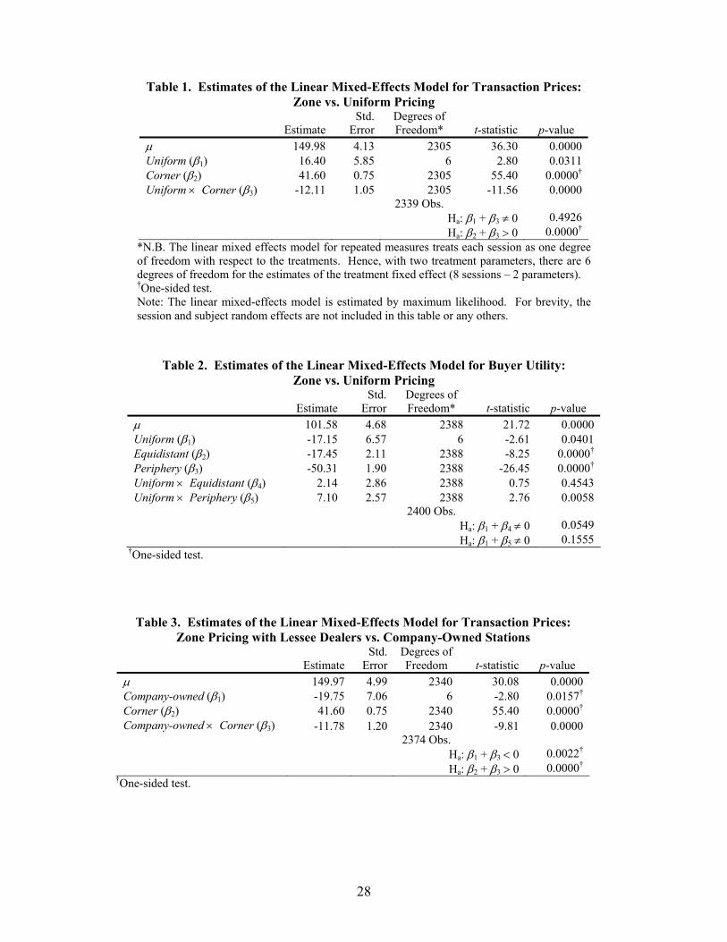
Finding 1: Retail transaction prices are statistically higher in the isolated areas than in the clustered area. Uniform pricing in the wholesale market increases retail transaction prices in the clustered area, but has no significant effect on transaction prices in the isolated areas. Evidence: The mixed effects estimation results presented in Table 1 provide the quantitative

support for this finding. The average retail transaction price with zone pricing at the wholesale

level is µ̂ = 149.98 at a station in the clustered area and 2ˆˆ βµ + = 191.58 in an isolated area, a

27.7% increase. This effect of location is highly significant ( 2β̂ = 41.60, p-value = 0.0000).

With uniform pricing in the wholesale market, the average retail transaction price is 1ˆˆ βµ + =

166.38 at a station in the center and 321ˆˆˆˆ βββµ +++ =195.87 in the corner. Again the effect of

location is highly significant ( 32ˆˆ ββ + = 29.49, p-value=0.0000). The uniform pricing treatment

effect of 1β̂ = 16.40 at center stations is statistically significant (p-value = 0.0311) and nontrivial

in economic terms—uniform pricing at the wholesale level increases retail transaction prices in

14

the clustered area by 10.9%. Transaction prices in the isolated stations are slightly higher with

uniform pricing than with zone pricing ( 31ˆˆ ββ + = 4.29), but this effect is statistically

insignificant (p-value = 0.4926).

Given the data generated by our experiment we are able to determine that high retail

prices in the isolated areas are not the result of high wholesale prices with zone pricing, but

rather the cause of high wholesale prices. Figure 4 plots average wholesale prices and average

posted retail prices by location for the first 300 periods when subjects are learning about the

competitive pressures or lack thereof. Notice that, unlike Figure 2, wholesale prices to corner

stations have a noticeable upward trend in the zone pricing treatment. Over the first 100 periods,

corner station retail prices are very high. As the refiners recognize that these isolated stations are

very profitable at those prices, the refiners use zone pricing to capture some of the rents from the

corner stations. The clustered area stands in rather marked contrast. As station prices tumble due

to the competition, wholesale prices also fall as the refiners use zone pricing to be more

competitive. Only after station prices stabilize around period 250 do wholesale prices start to

rise as refiners attempt to capture the retailer profits in the clustered area. Ultimately, the

refiners capture more of the profits with zone pricing, but not to the detriment of consumers.

Also, we are able to gain insight as to why uniform pricing in the wholesale market

actually increases transaction prices for consumers in the clustered area. Fundamentally, the

reason is that uniform wholesale pricing forces the refiner to forgo profits in the corner to be

competitive in the center. Thus refiners forced to sell at a uniform price have an incentive to

keep wholesale prices elevated relative to the central wholesale prices with zone pricing. This is

demonstrated in Figure 5, which plots the red refiner’s wholesale price and red retailer’s posted

price for the center red branded station and the average decision by their counterparts for one

session. At the beginning of the session, the red refiner’s price quickly plummets from 231 to

120 and the red center station (s, a) = (4, 4) eventually follows suit. The refiner observes that

there are substantial profits accruing at the red corner station (s, a) = (6, 6) and in period 176

raises the wholesale price to 200. When in period 190 the red center station restocks at the new

wholesale price of 200, the station owner is forced to raise the center station’s retail price. The

red retailer maintains a high price at the center location because it cannot compete with the other

central stations which have average retail prices below the red retailer’s wholesale price. As the

15

red station will not sell these higher-cost units, competition in the center is weakened and

gradually the prices of the other refiners and stations drift upwards. The end result is that

uniform pricing at the wholesale level stymies retail competition in the clustered center.

Moreover, we note that it only takes one refiner’s unilateral action to initiate this process of

mitigating competition.

Our second finding considers the effect of mandating uniform wholesale pricing on buyer

utility. The ability to collect direct measures of consumer welfare and conduct this analysis is

another major benefit of a laboratory study over a field study where such measures cannot be

collected. Again, we use a linear mixed-effects model to estimate the quantitative effects of the

treatment (Zone vs. Uniform Pricing) on buyer utility. We classify each buyer as one of three

types: interior, equidistant, and periphery. Interior buyers are those closest to the center stations.

These buyers originate at one of the following intersections: (4, 3), (4, 4), (4, 5), (3, 4), or (5, 4).

A buyer is equidistant from the center stations and at least one corner station if it originates at (4,

1), (4, 2), (4, 6), (4, 7), (1, 4), (2, 4), (6, 4), (7, 4), (3, 3), (3, 5), (5, 3) or (5, 5). All other buyers

are relatively isolated, being located closer to a corner station, and are categorized as periphery

buyers. The treatment effect, buyer types (Interior, Equidistant, and Periphery) and interaction

effects are modeled as zero-one fixed effects. The sessions are again treated as random effects,

ei, so that the model we estimate is

ittiti

ttiiit

PeripheryUniformttanEquidisUniform Periphery ttanEquidisUniformetyBuyerUtili

εβββββµ

+×+×+++++=

54

321

where ),0(~ 21σNei and ),0(~ 2

,2 iit N σε . The sessions are indexed by i and the repeated periods

by t (e.g., t = 301, 302, …, 600). BuyerUtilityit is the utility that the buyer achieved in the

market. We also include heteroskedastic errors by session in the maximum likelihood estimation

of the model.

Finding 2: Uniform pricing in the wholesale market decreases buyer welfare for the interior and equidistant buyers, but has no significant effect on periphery buyers. Evidence: Table 2 reports the quantitative support for this finding. The average buyer utility for

interior buyers with zone pricing is µ̂ = 101.58 but with uniform wholesale pricing, buyer

welfare drops by 1β̂− = 17.15, a 16.9% decrease that is statistically significant (p-value =

0.0491). With zone pricing, equidistant buyers are worse off than interior buyers because they

16

have further to travel to the lower-price center stations ( 2β̂ = –17.45, p-value = 0.0000).

However, with uniform wholesale pricing, the welfare for these buyers is even lower than

equidistant buyers in the zone pricing treatment ( 41ˆˆ ββ + = –15.01, p-value = 0.0549). The point

estimates indicate that periphery buyers are harmed by uniform pricing ( 51ˆˆ ββ + = –10.05), but

this effect is statistically insignificant (p-value = 0.1555).

These first two findings directly counter the claims that zone pricing harms consumers

and that uniform pricing would benefit consumers. Uniform pricing in the wholesale market

raises the actual prices that consumers pay and reduces the welfare to all buyers except those on

the periphery. Our next finding reports the impact of uniform wholesale pricing on station and

refiner profits.

Finding 3: Uniform pricing significantly increases station profits, but has no effect on refiner profits. Evidence: Figure 6 provides the qualitative support for this finding. Each marker represents the

profits for one station owner from both the center and corner stations plotted against the

associated refiner’s profits. It is clear from the figure that station owner profits increase

substantially with uniform wholesale pricing. The average station owner earns profits of 801

with zone pricing and 2304 with uniform pricing. For the quantitative support for this finding,

we use a Wilcoxon rank sum test to compare the total station owner profits of the four zone

pricing sessions with the total station owner profits of the four uniform sessions. We reject the

null hypothesis of equal station owner profits with a two-sided test (W = 26, n = 4, m = 4, p-value

= 0.0286). Average refiner profits are slightly lower with uniform pricing, 2616 versus 3006

with zone pricing, but a Wilcoxon rank sum test indicates that this difference is not statistically

significant (W = 17, n = 4, m = 4, p-value = 0.8857).

In sum, we find that uniform wholesale pricing (a) reduces consumer welfare by

increasing the prices that buyers pay at the clustered stations, relative to retail prices under zone

pricing, (b) has no statistical effect on consumer welfare and prices for buyers that are in isolated

areas, (c) increases station owner profits, and (d) has no statistical effect on refiner profits.

17

5.1.2 Zone Pricing (Lessee Dealers) versus Company-owned Stations

The effects of vertical integration are also rather striking. Figure 7 displays histograms of

the posted retail prices. The mode for the corner stations is 200 in both the zone and company-

owned treatments; however, there is considerably more mass in the left tail of the company-

owned treatments. The effect of vertical integration on retail prices is considerably more

conspicuous at the center stations. The entire distribution of posted prices shifts to the left with

company-owned stations. The mode with lessee dealers is only 120, whereas the mode is 150

under zone pricing with lessee dealers.

For our quantitative analysis, we estimate a linear mixed effects for transaction prices.

The treatment effect (Lessee Dealers with Zone Pricing vs. Company-Owned Stations) and

location effect (Center vs. Corner station) and an interaction effect are modeled as zero-one

fixed effects, while the 8 independent sessions and the 4 retailers within each session are

modeled as random effects.

Finding 4: Retail transaction prices with company-owned stations are statistically lower in both the clustered area and the isolated areas than in the zone pricing treatment. Evidence: The mixed effects estimation results presented in Table 3 provide the quantitative

support for this finding. With company-owned stations, the average retail transaction price is

1ˆˆ βµ + = 130.22 at a station in the center, which is 13.2% lower than transaction prices with

lessee dealers ( µ̂ = 149.97). This effect is statistically significant ( 1β̂ = -19.75, p-value =

0.0157). In isolated areas, transaction prices with company-owned stations are -( 31ˆˆ ββ + ) =

31.53 less than transaction prices with lessee dealers. This effect is also statistically significant

(p-value = 0.0022), reducing transaction prices by 16.5% from a level of 21ˆˆ βµ + = 191.58 with

lessee dealers to 3211ˆˆˆˆ βββµ +++ = 160.04 with company-owned stations.

Finding 4 reports the extent to which a double markup by refiners and stations raises the

prices that consumers pay vis-à-vis a single markup by company-owned stations. This finding

complements the field studies of Barron and Umbeck (1984) and Vita (2000) and a laboratory

study by Durham (2000), which also find that prices are lower with vertical integration than

18

without. Our next finding quantifies the additional utility buyers receive from eliminating the

double markup with company-owned stations.

Finding 5: Relative to the zone pricing treatment, pricing with company-owned stations increases buyer welfare for all types of buyers: interior, equidistant, and periphery. Evidence: Table 4 reports that with company-owned stations the utility of interior and

equidistant buyers increases by 1β̂ = 20.45 (p-value = 0.0241). (The point estimate for

equidistant buyers, 4β̂ , is small and highly insignificant.) The utility of periphery buyers

increases by 51ˆˆ ββ + = 25.94 (p-value = 0.0084). These absolute increases in buyer welfare

translate into percentage increases of 20.1%, 24.4%, and 50.6% in buyer welfare for the interior,

equidistant, and periphery buyers, respectively.

5.2 Dynamic Adjustments with Nonstationary Wholesale Costs

We now turn our attention to how prices dynamically adjust to nonstationary costs.

Figure 8 depicts wholesale costs, average retail prices, and average retailer costs (net of

10),,(

=ribas

eρ

) for the selling a unit from inventory in period t. It is clear that retail prices more

closely follow the station’s cost of gasoline than the wholesale costs. The noticeable lagged

response of retail prices to changes in wholesale costs is presumably due to the inventories of the

stations. In this subsection we investigate how retail prices adjust to changes in station costs. In

particular, we investigate whether station prices respond symmetrically or adjust faster to cost

increases than to decreases.

As a first step, we must determine whether a long run relationship exists between station

prices pt and costs ct (wholesale prices).29 If both pt and ct are nonstationary with a unit root, i.e.,

integrated of order 1, I(1), then we can operationalize the hypothesis of a long run (equilibrium)

relationship between pt and ct using the concept of cointegration developed by Engle and

Granger (1987). Station prices and costs are said to be cointegrated if a linear combination of the

two series is stationary, I(0). If pt and ct have a long run equilibrium relationship, then the short

run dynamics of the cointegrated system also have an error-correction representation. An error-

29 For ease of exposition we are dropping the location, retailer identity, and brand subscripts from per period prices and costs.

19

correction model of the first differences (∆pt and ∆ct) includes a term that reflects the current

“error” in the levels of pt and ct in achieving long-run equilibrium. To test whether prices adjust

asymmetrically or symmetrically to changes in cost, we follow Granger and Lee (1989) in

estimating a non-symmetric error correction model, namely,

tttttt zzpcp ξφφαα +++∆+∆=∆ +−−−− 12111211 ,

where ),0(~ 2σξ Nt , zt-1 is the error-correction term, and )0 ,max( 11 −+− = tt zz . If prices adjust

symmetrically, the speed of the adjustment to the long run equilibrium is captured

by 01 1 <<− φ , with .02 =φ If prices respond faster to cost increases than decreases, then

01 1 <<− φ and 02 >φ .

We begin this analysis by considering station prices and costs averaged across all

sessions and subjects for each station location (corner and center) and treatment (zone, uniform,

and company-owned), as depicted in Figure 8. Augmented Dickey-Fuller tests fail to reject the

null hypothesis for all series. Given that the each of series are found to be I(1), we now consider

whether a long run equilibrium exists between prices and costs for each location in each

treatment. This is our sixth finding.

Finding 6: With zone wholesale pricing and company-owned retail pricing, a long run relationship exists between station prices and station costs for both center and corner stations; however no such relationships exist with uniform pricing. Evidence: Table 5 reports the results of Johansen cointegration tests, which serve as the

qualitative support for this finding.30 Likelihood ratio (LR) tests of the number of cointegrating

equations indicate that there is 1 cointegrating equation at the 1% level of significance for both

corner and center stations with zone wholesale pricing and that there is 1 cointegrating equation

at the 5% level of significance for both corner and center stations with company-owned retail

pricing. However, the LR tests reject any cointegration with uniform pricing at the 5% level of

significance for either locale.

Finding 6 indicates that a long run equilibrium between station prices and costs with zone

wholesale pricing and with company-owned retail pricing. Shocks to costs, both positive and 30 Schwarz criteria indicate that a one period lag is superior to any other lag specification from two to thirty. The test assumption also assumes no deterministic trend in the data since none was included in the induced wholesale costs.

20

negative, are passed-through to customers via changes in station prices according to a stable long

run relationship between the two series. In contrast, we find that uniform wholesale pricing

breaks down the long run relationship between costs and prices at both center and corner

stations. This means that any relationship implied by a regression of prices on costs in levels is

spurious. Changes in costs still may lead to changes in prices, as Figure 8 faintly shows, but

there is no short run adjustment of prices toward a long run relationship with costs when costs

experience a shock. Uniform pricing purges the responsiveness of retail prices to cost changes,

the negative implication being that when wholesale costs fall, retail prices do not follow. This

also means that retail prices are insulated to increases in wholesale costs, but we also observe in

Finding 2 that uniform wholesale pricing generates high retail prices in the clustered area.

Our seventh finding addresses the “rockets and feathers” phenomenon in the retail

gasoline industry with zone wholesale pricing (7a) and company-owned retail pricing (7b),

where a long run equilibrium relationship exists.

Finding 7a: Station prices in the clustered area adjust quickly and asymmetrically to changes in costs with zone pricing. Station prices in isolated areas adjust more slowly, but symmetrically to changes in costs. Evidence: Table 6 and Figure 9 provide the support for this finding. Table 6 reports the

estimates of the error-correction model for the average station prices and costs across all sessions

and subjects by treatment. The error-correction term is highly significant and is largely

responsible for explaining the adjustment of prices (p-value < 0.0001 for both center and corner

stations). When the error-correction term is positive (i.e., costs are lower relative to what is

specified in the long run equilibrium given prices), the speed of adjustment for center stations is

considerably slower ( 21ˆˆ φφ + = -0.176 + 0.128 = -.048) than when error-correction term is

negative ( 1̂φ = -0.176). Figure 9 plots the adjustment of prices to positive and negative cost

shocks of 10 experimental dollars. For the center stations, over 90% of an increase in costs is

reflected in the price in just 11 periods (or just 18.7 seconds of experiment time), but in the same

amount of time only 40% of a decrease in costs is passed-through. In fact, it takes 45 periods (or

76.5 seconds) for 90% of a cost decrease to be reflected in the price at center stations. The speed

of adjustment for corner stations is slower than for center stations ( 1̂φ = -0.047) and is symmetric

( 2̂φ is statistically insignificant with a p-value = 0.1650).

21

Finding 7b: With company-owned retail pricing, station prices adjust symmetrically and much more slowly to changes in station costs. Evidence: As reported in Table 6, the error-correction term 1̂φ is significant for both center and

corner stations (p-value = 0.0001 and 0.0353, respectively), but 2̂φ is statistically insignificant

(p-values = 0.9522 and 0.7719). Figure 9 indicates that the adjustment of prices to positive and

negative cost shocks is rather slow. For the center stations, 90% of an increase in costs is

reflected in the price in 123 periods, and at corner stations it takes 152 periods for 90% of a cost

increase to be reflected in the price.

Having found at an aggregate level that prices adjust asymmetrically at the center stations

with zone wholesale pricing, we continue to exploit our dataset to investigate asymmetric price

responses to costs. First, we estimate error-correction models for the center stations at the

session level and then for each individual station owner in each of the four zone pricing

sessions.31 In the interest of brevity, we focus on the estimates at the session level but only

classify the individual station owners by whether 2̂φ is (a) statistically positive, (b) statistically

not different than zero, (c) statistically negative, or by (d) not having cointegrated prices and

costs.

Finding 8: At the session level, station prices in the clustered area adjust asymmetrically to changes in costs with zone pricing. Individual station owners are predominantly and equally classified as one of two behavioral types: asymmetric and symmetric adjusters.

Evidence: Table 8 reports that prices rise faster than they fall in response to cost changes in three

of the four sessions ( 2̂φ > 0 with p-values = 0.0051, 0.0740, and 0.0000). In the fourth session,

prices actually fall faster than they rise ( 2̂φ < 0 with p-value = 0.0107). The sessions that adjust

faster to cost increases contain at least one station owner who is classified as an asymmetric

adjuster with 2̂φ statistically greater than 0, as reported in Table 8. The fourth session contains

three symmetric adjusters and one station owner who decreases prices faster than he increases 31 Augmented Dickey-Fuller tests for all series fail to reject the null hypothesis of a unit root, and unless otherwise noted, Johansen cointegration tests indicate that all pairs of price and cost series are cointegrated. The Schwarz criteria also continue to indicate that 1 lag is superior to any other lag specification.

22

them in response to cost changes. Of the 16 station owners, 6 respond faster to cost increases

than to decreases and 6 respond symmetrically.

Finding 8 begs the question as to whether there are any reasons why some station owners

adjust asymmetrically while others adjust symmetrically. Using a meta-analysis of several

industries, Peltzman (2000) uncovers a stylized fact that more volatile input prices are correlated

with less price asymmetries. In our laboratory experiment we can directly test whether the

volatility of wholesale prices set by refiners affects the price adjustment behavior of station

owners. This comprises our final finding.

Finding 9: The volatility of wholesale prices is uncorrelated with whether or not a station owner adjusts prices asymmetrically or symmetrically. However, during regimes of increasing wholesale costs, more volatile wholesale prices are correlated with station owners who respond more quickly to wholesale price increases than to wholesale price decreases. Evidence: Using a Wilcoxon rank sum statistic we test whether the variance of the change in

wholesale prices is correlated with a station owner being classified as an asymmetric ( 2̂φ > 0) or

symmetric ( 2̂φ = 0) price adjuster. Specifically, we compare the variance of wholesale price

changes for periods 601-1200 for the 6 asymmetric price adjusters to the 6 symmetric price

adjusters and find that there is no statistical difference (W = 43, n = 6, m = 6, p-value = 0.5887).

However, if we separately measure the variance of price changes when wholesale costs are rising

(periods 778-853 and 1053-1200), volatility of wholesale prices is larger for the asymmetric

price adjusters than for symmetric price adjusters (W = 27, n = 6, m = 6, p-value = 0.0649).

When wholesale costs are falling in periods 601-777 and 854-1052, there is no statistical

difference in the volatility of wholesale prices for the different retail types (W = 43, n = 6, m = 6,

p-value = 0.5887).

The implication of Finding 9 is that refiners who have greater volatility in wholesale

prices during periods of rising crude oil costs cause their station owners to increases their prices

more quickly than these same individuals decrease their retail prices when wholesale prices and

oil prices are falling.

23

6. Conclusion

The gasoline industry is an intricate system, making the implications of policies such as

prohibiting zone pricing and vertical integration unclear from anecdotal evidence alone.

However, such topics are regularly debated in the political arena. Consumers and media

routinely scrutinize retail gasoline prices looking for evidence of anticompetitive behavior. The

sheer magnitude and social interest in this market has led numerous research studies of the

industry. Unfortunately, this field research must rely on incomplete information. In this study

we detail a laboratory investigation of the gasoline industry, focusing specifically on uniform

pricing at the wholesale level, divorcement, and asymmetric retail price responses to cost shocks.

Our study provides a series of insights into the effect of zone pricing. In many situations

our results provide support for hypotheses formalized by previous researchers. First, prices in

relatively isolated areas are higher than prices in areas with a clustering of stations. Contrary to

the claims expressed by proponents of uniform pricing legislation, uniform wholesale pricing

actually increases prices in the more competitive area and simultaneously does not alter prices in

more isolated geographic areas that are less competitive. Due to this behavior, uniform pricing

actually reduces the welfare of buyers who are closest to the center area, as well as those who are

on the border of the center and isolated areas. The buyer losses are not the refiners’ gains. In

fact we find that refiners’ profits are unaffected by the uniform pricing. Instead, it is the retailers

that are extracting surplus from the consumers. The data offer a simple explanation for this

result. Under uniform pricing, the refiners offer a price that is above the center area zone

wholesale price and below the isolated area zone wholesale price. These refiners are balancing

extracting economic rents from the isolated stations and remaining viable in the competitive,

center area. Thus, a refiner’s gains in the center area, due to higher wholesale prices, are offset

by reduced earnings in the isolated markets where wholesale prices have decreased and profits

are unchanged. With uniform pricing the retailers do not gain a profit margin in the center area

but do receive a larger margin in the isolated regions where retail prices are unchanged but

wholesale prices have declined.

On the issue of divorcement we find that company-owned stations eliminate the double

markup of prices. From this we can conclude that divorcement legislation harms consumers. All

buyers, in clustered or isolated areas, pay lower prices and have substantially higher utility when

stations are company-owned. This price finding in the laboratory (buyer utility cannot be

24

directly measured in field studies) affirms the results from field studies, lending credence to our

other findings.

Numerous studies have demonstrated an asymmetry in gasoline price responses. In the

laboratory we are able to investigate this pattern while controlling for collusion, menu costs, and

buyer search. With zone pricing, the practice in place when previous studies evaluated

asymmetric price responses, we find that retail prices and retail costs are cointegrated, i.e., a long

term equilibrium relationship exists between the two series. Our data indicate that prices in the

center area adjust more quickly to costs increases than to cost decreases, but we find that in

isolated areas price responses are symmetric. At the market (session) level we find that

responses are influenced by the idiosyncrasies of individual retailers, some of whom respond

symmetrically and some of whom respond asymmetrically. Further, a retailer’s type is not

correlated with the volatility of its wholesaler’s prices. However, retailers who observe more

volatile wholesale prices during periods of increasing wholesale costs (or world oil prices) are

more likely to respond asymmetrically. With company-owned stations, prices adjust

symmetrically to cost shocks. Further, this response is substantially slower in the company-

owned treatment than with zone pricing.

In addition to benefiting retailers at the expense of consumers, another effect of uniform

pricing is the destruction of the long term relationship between retail prices and costs. Formally,

we find that with uniform wholesale pricing, retail costs and prices are not cointegrated and

therefore any reduction in wholesale costs, say due to changes in the world price for oil, would

not necessarily be reflected in retail prices.

As with any empirical study, the inherent specificity of a data set is determined by such

details as the environment and institution, and raises the typical issues of inferring broader

implications from the results. Further research would be useful in examining how the exogenous

location and number of stations, as well as endogenous and costly entry and exit, affect our

findings. Along the lines of Shepard (1993), it would also be useful to explore the endogenous

formation of vertical relationships in laboratory markets.

25

References

Bacon, Robert W., “Rockets and Feathers: The Asymmetric Speed of Adjustment of UK Retail

Gasoline Prices to Cost Changes.” Energy Economics v13, 1991, pp. 211-8.

Barron, John M. and Umbeck, John R., “The Effects of Different Contractual Arrangements: The

Case of Retail Gasoline Markets.” Journal of Law and Economics v27, 1984, pp. 313-28.

Borenstein, Severin and Shepard, Andrea, “Dynamic Pricing in Retail Gasoline Markets.”

RAND Journal of Economics v27, 1996, pp. 429-51.

Borenstein, Severin; Cameron, A. Colin and Gilbert, Richard, “Do Gasoline Prices Respond

Asymmetrically to Crude Oil Price Changes?” Quarterly Journal of Economics v112,

1997, pp. 305-39.

Bulow, Jeremy; Fischer, Jeffrey; Creswell, Jay and Taylor, Christopher, “U.S. Midwest Gasoline

Pricing and the Spring 2000 Price Spike.” The Energy Journal, v24 (3), 2003, pp. 121-

149.

Castanias, Rick and Johnson, Herb, “Gas Wars: Retail Gasoline Fluctuations.” Review of

Economics and Statistics v75, 1993, pp. 171-74

Chouinard, Hayley and Perloff, Jeffrey M., “Gasoline Price Differences: Taxes, Pollution

Regulations, Mergers, Market Power, and Market Conditions.” Working Paper,

University of California at Berkeley, 2001.

Comanor, William and Riddle, Jon, “The Costs of Regulation: Branded Open Supply and

Uniform Pricing of Gasoline.” International Journal of the Economics of Business, v10

(2), 2003, pp. 123-144.

Douglas, Elizabeth, “Station Owners Pump Fists at Oil Companies,” L. A. Times, May 7, 2003.

Durham, Yvonne, “An Experimental Examination of Double Marginalization and Vertical

Relationships.” Journal of Economic Behavior and Organization, v42 (2), 2000, pp.207-

229.

Engle, Robert and Granger, Clive, “Co-integration and Error Correction: Representation,

Estimation, and Testing.” Econometrica v55, 1987, pp. 251-76

Granger, Clive and Lee, T. H., “Investigation of Production, Sales and Inventory Relationships

Using Multicointegration and Non-symmetric Error Correction Models.” Journal of

Applied Econometrics v4, December 1989, pp. S145-59.

Hastings, Justine, “Prepared Statement Before the Committee on Governmental Affairs,”

26

Permanent Subcommittee on Investigations, United States Senate, May 2, 2002a.

Hastings, Justine, “Vertical Relationships and Competition in Retail Gasoline Markets.”

Working Paper, Dartmouth University, 2002b.

Heywood, John S.; Monaco, Kristen, and Rothschild, R., “Spatial Price Discrimination and

Merger: The N-Firm Case.” Southern Economic Journal v67 2001, pp. 672-84.

Hotelling, Harold, “Stability in Competition.” Economic Journal v39, 1929, pp. 41-57.

Irmen, Andreas and Thisse Jacques-Fracois, “Competition in Multi-Characteristic Space:

Hotelling Was Almost Right.” Journal of Economic Theory v78, 1998, pp. 76-102.

Isaac, Mark; Oaxaca, Ronald and Reynolds, Stanley, “Competition and Pricing in the Arizona

Gasoline Market.” working paper, University of Arizona, 1998.

Johnson, Ronald, “Search Costs, Lags, and Prices at the Pump.” Review of Industrial

Organization v20, 2002, pp. 33-50.

Lafontaine, Francine and Slade, Margaret E., “Retail Contracting: Theory and Practice.” Journal

of Industrial Economics v45, 1997, pp. 1-25.

Lockyer, Bill. “Report on Gasoline Pricing in California.” Office of the Attorney General of the

State of California, May 2000.

Longford, N. T., Random Coefficient Models. New York: Oxford University Press, 1993.

Manuszak, Mark, “The Impact of Upstream Mergers on Retail Gasoline Markets.” working

paper, Carnegie Mellon University, 2001.

Maskin, Eric and Tirole, Jean, “A Theory of Dynamic Oligopoly, II: Price Competition, Kinked

Demand Curves, and Edgeworth Cycles.” Econometrica v56, 1988, pp. 571-99.

Peltzman, Sam, “Prices Rise Faster Than They Fall.” Journal of Political Economy v108, 2000,

pp. 466-502.

Pinkse, Joris; Slade, Margaret E., and Brett, Craig, “Spatial Price Competition: A

Semiparametric Approach.” Econometrica v70, 2002, pp. 1111-53.

Reilly, Barry and Witt, Robert, “Petrol Price Asymmetries Revisited.” Energy Economics v20,

1998, pp. 297-308.

Rey, Patrick and Stiglitz, Joseph. “The Role of Exclusive Territories in Producers' Competition.”

RAND Journal of Economics v26, 1995, pp. 431-51.

Salop, S., “Monopolistic Competition With Outside Goods,” Bell Journal of Economics v10,

1979, pp. 141-156.

27

Scholer, Klaus, “Consistent Conjectural Variations in a Two-Dimensional Spatial Market.”

Regional Science and Urban Economics v23, 1993, pp. 765-78.

Shepard, Andrea, “Contractual Form, Retail Price, and Asset Characteristics in Gasoline

Retailing.” RAND Journal of Economics v24, 1993, pp. 58-77.

Slade, Margaret E., “Vancouver’s Gasoline-Price Wars: An Empirical Exercise in Uncovering

Supergame Strategies.” Review of Economic Studies v59, 1992, pp. 257-76.

Slade, Margaret E., “Strategic Motives for Vertical Separation: Evidence from Retail Gasoline

Markets.” Journal of Law, Economics, and Organization v14, 1998, pp. 84-113.

Smith, Vernon L., “Microeconomic Systems as an Experimental Science,” American Economic

Review v72, 1982, pp. 923-55.

Smith, Vernon L., “Economics in the Laboratory.” Journal of Economic Perspectives v8, 1994,

pp. 113-31.

Vandenbosch, Mark and Charles Weinberg, “Product and Price Competition in a Two-

Dimensional Vertical Differentiation Model.” Marketing Science v14, 1995, pp. 224-49.

Veendorp, E. and Majeed Anjum, “Differentiation in a Two-Dimensional Market.” Regional

Science and Urban Economics v25, 1995, pp. 75-83.

Vita, Michael G., “Regulatory Restrictions on Vertical Integration and Control: The Competitive

Impact of Gasoline Divorcement Policies.” Journal of Regulatory Economics v18, 2000,

pp. 217-33.

28

Table 2. Estimates of the Linear Mixed-Effects Model for Buyer Utility: Zone vs. Uniform Pricing

Estimate

Std. Error

Degrees of Freedom*

t-statistic

p-value

µ 101.58 4.68 2388 21.72 0.0000 Uniform (β1) -17.15 6.57 6 -2.61 0.0401 Equidistant (β2) -17.45 2.11 2388 -8.25 0.0000† Periphery (β3) -50.31 1.90 2388 -26.45 0.0000† Uniform × Equidistant (β4) 2.14 2.86 2388 0.75 0.4543 Uniform × Periphery (β5) 7.10 2.57 2388 2.76 0.0058

2400 Obs. Ha: β1 + β4 ≠ 0 0.0549 Ha: β1 + β5 ≠ 0 0.1555

†One-sided test.

Table 1. Estimates of the Linear Mixed-Effects Model for Transaction Prices: Zone vs. Uniform Pricing

Estimate

Std. Error

Degrees of Freedom*

t-statistic

p-value

µ 149.98 4.13 2305 36.30 0.0000 Uniform (β1) 16.40 5.85 6 2.80 0.0311 Corner (β2) 41.60 0.75 2305 55.40 0.0000† Uniform × Corner (β3) -12.11 1.05 2305 -11.56 0.0000

2339 Obs. Ha: β1 + β3 ≠ 0 0.4926 Ha: β2 + β3 > 0 0.0000†

*N.B. The linear mixed effects model for repeated measures treats each session as one degree of freedom with respect to the treatments. Hence, with two treatment parameters, there are 6 degrees of freedom for the estimates of the treatment fixed effect (8 sessions – 2 parameters). †One-sided test. Note: The linear mixed-effects model is estimated by maximum likelihood. For brevity, the session and subject random effects are not included in this table or any others.

Table 3. Estimates of the Linear Mixed-Effects Model for Transaction Prices: Zone Pricing with Lessee Dealers vs. Company-Owned Stations

Estimate

Std. Error

Degrees of Freedom

t-statistic

p-value

µ 149.97 4.99 2340 30.08 0.0000 Company-owned (β1) -19.75 7.06 6 -2.80 0.0157† Corner (β2) 41.60 0.75 2340 55.40 0.0000† Company-owned × Corner (β3) -11.78 1.20 2340 -9.81 0.0000

2374 Obs. Ha: β1 + β3 < 0 0.0022† Ha: β2 + β3 > 0 0.0000†

†One-sided test.

29

Table 5. Johansen Cointegration Tests of the Equation: pt = β0 + β1ct Treatment and Location

Eigenvalue

LR

statistic

5% Critical Value

1% Critical Value

No. of Cointegrating

Equations Zone Pricing, Center Stations 0.087171 55.27 19.96 24.60 0** 0.001219 0.73 9.24 12.97 1 Zone Pricing, Corner Stations 0.054853 35.43 19.96 24.60 0** 0.002834 1.70 9.24 12.97 1 Uniform Pricing, Center Stations 0.027930 18.03 19.96 24.60 0 0.001816 1.09 9.24 12.97 1 Uniform Pricing, Corner Stations 0.016531 10.91 19.96 24.60 0 0.001572 0.94 9.24 12.97 1 Company-Owned, Center Stations 0.042158 26.86 19.96 24.60 0* 0.001847 1.11 9.24 12.97 1 Company-Owned, Corner Stations 0.036239 22.91 19.96 24.60 0* 0.001403 0.84 9.24 12.97 1

* Denotes rejection of the hypothesis at 5% significance level. ** Denotes rejection of the hypothesis at 1% significance level.

Table 4. Estimates of the Linear Mixed-Effects Model for Buyer Utility: Zone Pricing with Lessee Dealers vs. Company-Owned Stations

Estimate

Std. Error

Degrees of Freedom*

t-statistic

p-value

µ 101.59 5.82 2388 17.44 0.0000 Company-owned (β1) 20.45 8.26 6 2.47 0.0241† Equidistant (β2) -17.45 2.11 2388 -8.25 0.0000† Periphery (β3) -50.32 1.90 2388 -26.44 0.0000† Company-owned × Equidistant (β4) 0.05 3.11 2388 0.02 0.4940† Company-owned × Periphery (β5) 5.49 2.81 2388 1.96 0.0253†

2400 Obs. Ha: β1 + β4 > 0 0.0216† Ha: β1 + β5 > 0 0.0084†

†One-sided test.

30

Table 6. Estimates of Error-Correction Model for ∆pt

Estimate

Std. Error

t-statistic

p-value

Zone Pricing All Center Stations ∆ct-1 -0.098 0.052 -1.87 0.0620 ∆pt-1 0.009 0.039 0.23 0.8182 zt-1 -0.176 0.026 -6.82 0.0000

+−1tz 0.128 0.035 3.67 0.0003

2R = 0.10

Zone Pricing All Corner Stations ∆ct-1 0.022 0.044 0.49 0.6243 ∆pt-1 -0.001 0.040 -0.23 0.8182 zt-1 -0.047 0.010 -4.60 0.0000

+−1tz 0.020 0.014 1.39 0.1650

2R = 0.06 Company-Owned All Center Stations

∆ct-1 0.052 0.066 0.79 0.4298 ∆pt-1 0.092 0.040 2.28 0.0230 zt-1 -0.065 0.016 -3.98 0.0001

+−1tz -0.002 0.026 -0.06 0.9522

2R = 0.05 Company-Owned All Corner Stations

∆ct-1 -0.006 0.066 -0.09 0.9283 ∆pt-1 0.038 0.041 0.92 0.3579 zt-1 -0.039 0.018 -2.11 0.0353

+−1tz 0.007 0.025 0.29 0.7719

2R = 0.01

31

Table 7. Estimates of Error-Correction Model for ∆pt by Session for Center Stations

Estimate

Std. Error

t-statistic

p-value

Session 1 ∆ct-1 -0.048 0.047 -1.01 0.3129 ∆pt-1 0.008 0.040 0.20 0.8415 zt-1 -0.152 0.027 -5.65 0.0000

+−1tz 0.101 0.036 2.81 0.0051

2R = 0.07

Session 2 ∆ct-1 -0.177 0.069 -2.55 0.0110 ∆pt-1 -0.042 0.040 -1.05 0.2941 zt-1 -0.086 0.026 -3.32 0.0010

+−1tz 0.061 0.034 1.79 0.0740

2R = 0.04 Session 3 ∆ct-1 -0.174 0.051 -3.41 0.0007 ∆pt-1 0.015 0.039 0.38 0.7041 zt-1 -0.244 0.029 -8.49 0.0000

+−1tz 0.178 0.041 4.37 0.0000

2R = 0.13

Session 4 ∆ct-1 -0.127 0.047 -2.68 0.0076 ∆pt-1 0.002 0.038 0.04 0.9681 zt-1 -0.086 0.014 -6.19 0.0000

+−1tz -0.062 0.024 -2.56 0.0107

2R = 0.10

32

Table 8. Types of Station Owners Asymmetric

2̂φ > 0 Symmetric

2̂φ = 0 Asymmetric

2̂φ < 0 pt and ct are

not cointegrated

Session 1

X* No. Subjects 3 1

Session 2 X

No. Subjects 1 1 2** Session 3 X

No. Subjects 2 1 1 Session 4 X

No. Subjects 3 1 Totals 6 6 2 2

*See Table 7 for estimates. **The refiners for these station owners maintained somewhat high prices that did not vary much over time.

1st St.

2nd St.

3rd St.

4th St.

5th St.

1st Ave. 2nd Ave. 3rd Ave. 4th Ave. 5th Ave. 6th Ave. 7th Ave.

6th St.

7th St.

1),4,4( 1b ρ

1),2,2( 1b ρ

3),4,4( 3b ρ

4),4,4( 4b ρ

3),6,2( 3b ρ

4),6,6( 4b ρ2

),2,6( 2b ρ

2),4,4( 2b ρ

1st St.

2nd St.

3rd St.

4th St.

5th St.

1st Ave. 2nd Ave. 3rd Ave. 4th Ave. 5th Ave. 6th Ave. 7th Ave.

6th St.

7th St.

1),4,4( 1b ρ

1),2,2( 1b ρ

3),4,4( 3b ρ

4),4,4( 4b ρ

3),6,2( 3b ρ

4),6,6( 4b ρ2

),2,6( 2b ρ

2),4,4( 2b ρ

Figure 1. Geographic Depiction of the Laboratory Retail Gasoline Market

33

Zone Pricing to Corner Stations

90

110

130

150

170

190

210

301 326 351 376 401 426 451 476 501 526 551 576Period

Pric

e

Wholesale Cost

Uniform Pricing to Center and Corner Stations

90

110

130

150

170

190

210

301 326 351 376 401 426 451 476 501 526 551 576

Period

Pric

e

Wholesale Cost

Zone Pricing to Center Stations

90

110

130

150

170

190

210

301 326 351 376 401 426 451 476 501 526 551 576Period

Pric

e

Wholesale Cost

Figure 2. Average Wholesale Prices by Session

Corner Stations with Uniform Pricing

0200400600800

10001200140016001800

110 130 150 170 190 210 230 250 MorePrice Bins

Freq

uenc

y

Corner Stations with Zone Pricing

0200400600800

10001200140016001800

110 130 150 170 190 210 230 250 MorePrice Bins

Freq

uenc

y

Center Stations with Zone Pricing

0200400600800

10001200140016001800

110 130 150 170 190 210 230 250 MorePrice Bins

Freq

uenc

y

Center Stations with Uniform Pricing

0200400600800

10001200140016001800

110 130 150 170 190 210 230 250 MorePrice Bins

Freq

uenc

y

Figure 3. Histograms of Station Posted Prices: Zone vs. Uniform Pricing

34

100

120

140

160

180

200

220

1 26 51 76 101 126 151 176 201 226 251 276

Period

Pric

e

Corner Station PriceWholesale Price to Corner StationsCenter Station PriceWholesale Price to Center Stations

Figure 4. Average Wholesale and Station Prices with Zone Pricing in Periods 1-300

100

120

140

160

180

200

220

240

260

1 26 51 76 101 126 151 176 201 226 251 276 301 326 351 376 401

Period

Pric

e

Red Station PriceRed Wholesale PriceAverage Other Station PricesAverage Other Wholesale Prices

Figure 5. Example of How High Prices Arise in the Center with Uniform Wholesale Prices

35

0

1000

2000

3000

4000

5000

6000

7000

0 1000 2000 3000 4000 5000 6000 7000

Station Profits

Ref

iner

Pro

fits Zone, Session 1

Zone, Session 2Zone, Session 3Zone, Session 4Uniform, Session 1Uniform, Session 2Uniform, Session 3Uniform, Session 4

Figure 6. Station vs. Refiner Profits for Periods 301-600

Corner Stations with Zone Pricing

0200400600800

10001200140016001800

110 130 150 170 190 210 230 250 MorePrice Bins

Freq

uenc

y

Center Stations with Zone Pricing

0200400600800

10001200140016001800

110 130 150 170 190 210 230 250 MorePrice Bins

Freq

uenc

y

Company-Owned Center Stations

0200400600800

10001200140016001800

110 130 150 170 190 210 230 250 MorePrice Bins

Freq

uenc

y

Company-Owned Corner Stations

0200400600800

10001200140016001800

110 130 150 170 190 210 230 250 MorePrice Bins

Freq

uenc

y

Figure 7. Histograms of Station Posted Prices: Zone Pricing (Lessee Dealer) vs. Company-Owned Stations

36

Zone Pricing to Center Stations

50

100

150

200

250

601 651 701 751 801 851 901 951 1001 1051 1101 1151Period

Pric

e

PricesCostsWholesale Cost

Zone Pricing to Corner Stations

50

100

150

200

250

601 651 701 751 801 851 901 951 1001 1051 1101 1151Period

Pric

e

PricesCostsWholesale Cost

Uniform Pricing to Corner Stations

50

100

150

200

250

601 651 701 751 801 851 901 951 1001 1051 1101 1151Period

Pric

e

PricesCostsWholesale Cost

Uniform Pricing to Center Stations

50

100

150

200

250

601 651 701 751 801 851 901 951 1001 1051 1101 1151Period

Pric

e

PricesCostsWholesale Cost

Company-Owned Pricing to Corner Stations

50

100

150

200

250

601 651 701 751 801 851 901 951 1001 1051 1101 1151Period

Pric

e

PricesCostsWholesale Cost

Company-Owned Pricing to Center Stations

50

100

150

200

250

601 651 701 751 801 851 901 951 1001 1051 1101 1151Period

Pric

e

PricesCostsWholesale Cost

Figure 8. Station Prices and Costs in Periods 601-1200

37

-10

-8

-6

-4

-2

0

2

4

6

8

10

1 2 3 4 5 6 7 8 9 10 11 12 13 14 15 16 17 18 19 20 21 22 23 24 25 26 27 28 29 30Periods

Adj

ustm

ent o

f Pri

ces t

o C

ost D

ecre

ases

C

ost I

ncre

ases Center Stations

Corner Stations

Zone Pricing Treatment

-10

-8

-6

-4

-2

0

2

4

6

8

10

1 2 3 4 5 6 7 8 9 10 11 12 13 14 15 16 17 18 19 20 21 22 23 24 25 26 27 28 29 30Periods

Adj

ustm

ent o

f Pri

ces t

o C

ost D

ecre

ases

C

ost I

ncre

ases

Center StationsCorner Stations

Company-Owned Treatment

Figure 9. Adjustment of Station Prices to a 10 Experimental Dollar Innovation in Cost