EPPP DP No. 2014-03 The Determinants of Margins in Gasoline Markets Thomas Porcher Simon Porcher Mars 2014 D

ISC

US

SIO

N P

AP

ER S

ERIE

S

Chaire Economie des Partenariats Public-Privé Institut d’Administration des Entreprises

The Determinants of Margins in Gasoline Markets1

Thomas Porcher ESG Management School

Simon Porcher

Université Paris Est Créteil, IRG

Abstract

When studying oligopolies, a tension exists between models supporting tacit collusion and those supporting the non-collusive behavior of firms. Using a panel on retail fuel margins in France over more than twenty years, we find mitigated evidence of collusive behavior in the retail gasoline industry. On the one hand, we find lower margins when demand is expected to increase in the next period, which is a standard prediction for the non-cooperative models. On the other hand, we also find evidence of tacit collusion as margins respond to input cost changes in the manner that the tacit collusion models predict: margins decline when the expected marginal cost increases. Our results leave open the question of collusion in the retail gasoline market.

!!!!!!!!!!!!!!!!!!!!!!!!!!!!!!!!!!!!!!!!!!!!!!!!!!!!!!!!!!!!!1 Corresponding author: thomasporcher@hotmail.com. Thomas Porcher is an associate professor of economics at ESG Management School. Simon Porcher is an assistant professor at Université Paris Est, IRG. All remaining errors are ours.

1. Introduction

Gasoline markets have been a focus of intensive research within the petroleum industry. Researchers and governments are intrigued by the incomplete pass-through between crude oil price changes and retail prices, market power at the retail level and regulation. At the crossroads of the determinants of margins and the study of collusive behaviors, few studies have focused on the link between margins and future demand when marginal costs are not stable (see Houde [2011] for a literature review and Borenstein and Shepard [1996] for the baseline article on this subject).

Numerous models have been developed to empirically distinguish between collusive and non-collusive pricing behaviors. In supergame models with repeated play, firms can sustain implicit collusion by adjusting their current margins in response to changes in expected demand. For example, in the Haltiwanger-Harrington [1991] model, a firm has incentives to deviate from the implicit collusion when demand increases because near-term profits are weighted more heavily when evaluating a firm’s present and future global profits. Margins therefore respond positively to changes in expected demand, ceteris paribus. Such an argument is similar to the “price wars during booms” prediction of Rotemberg and Saloner [1986]. In the gasoline market, marginal costs – proxied by the crude oil price or the price after refining – move regularly. Collusion is more difficult to sustain when demand is declining or costs are increasing.

Our approach exploits the insights from the theoretical background of these supergame models to test for collusive pricing in retail gasoline markets by focusing on retail margins in the industry. Margins in the gasoline markets are interesting to study because they can have strong welfare impacts on citizens. Our study clearly computes price-cost margins at the national level using monthly data from 1990 onward in France. Due to the structure of the gasoline market, where demand and retail prices are highly predictable in the short term, the industry appears to be a natural candidate for a test of the level of collusion.

Our results provide insight on the magnitude of the impact of collusive behavior in gasoline markets. In our simplest estimates, an increase in the expected demand by 10 kilotons per day decreases margins by 0.65 cents, representing an elasticity of -0.5. Such a level of elasticity reveals a non-collusive behavior: when demand is expected to increase in the next period, gas stations decrease their margins to attract consumers. However, when future marginal costs are expected to decrease, current margins are higher, as predicted by the collusive models. Indeed, in tacit collusion, margins increase with expected future collusive profits. When marginal costs are expected to rise in the next period, the collusive profits are expected to decline and thereby lower the future cost of punishment. Our results show that on average, gasoline retailers do not act as the tight oligopoly that we might imagine, even though they tend to increase their overall margins.

In the following section, we present a literature review on models of price dynamics. In Section 3, we discuss the data and the econometric estimations. Section 5 presents the results. A brief conclusion follows.

2. Theoretical Background

Our empirical model is built on several theoretical assumptions drawn from collusion models. As in Borenstein and Shepard [1996], we assume that margins respond to current and future input prices and to changes in demand conditions. This assumption is based on two articles on supergame models in tacit collusion. In the “price wars during booms” model developed by Rotemberg and Saloner [1986], firms sustain implicit collusion by adjusting current margins in response to anticipated changes in demand. In this model, colluding oligopolies are likely to behave more competitively in periods of high demand because the gains from defection in the current period are high relative to the expected future cost of being punished for the defection. Thus, increases in demand lower the oligopoly’s prices monotonically. The oligopoly only increases output in response to higher demand while keeping price constant. In this case, profits increase when demand goes up. Therefore, a deviating firm can capture a share of an unusually large market by decreasing prices. The highest collusive margins will be higher in period t than in t-1.

Haltiwanger-Harrington [1991] formulate a model in which a firm has incentives to deviate from the implicit collusion when demand increases because the near-term profits are weighted more heavily in evaluating the firm’s present and future global profits. In this model, margins respond positively to changes in expected demand, ceteris paribus. As noted by Borenstein and Shepard [1996], both models imply that margins are affected by expectations about future marginal costs. When input prices are expected to rise, the expected marginal profits will decline and it will reduce the potential loss from future punishment. Therefore, a firm that expects marginal cost to increase has higher incentives to defect in the current period and thus to decrease margins.

However, those theoretical results are reversed when there are switching costs for consumers. Klemperer [1987] develops a model in which consumers are loyal to their gas stations, thus leading firms to set prices that attract consumers in the next period. In the first period, stations want to attract consumers to sell to them in the next period, especially if demand is expected to increase in the next period. If demand remains the same and marginal costs are expected to rise, margins would decrease tomorrow, resulting in higher margins today. The model implies that margins are lower when demand is increasing and higher when cost is increasing.

Price dynamics can also be explained by Edgeworth cycles (Maskin and Tirole, [1988]). In this formulation, prices follow an asymmetric cycle in which price increases are fast and large and are then followed by a sequence of small decreases. In this game of oligopolistic price competition, asymmetric price cycles are generated from equilibrium behavior: firms repeatedly steal market demand from one another by cutting their prices down to marginal cost. Firms then sequentially increase prices back to the top of the cycle and begin undercutting again. As summarized by Noel [2011], the empirical literature strongly favors the theory that the asymmetric price cycles in retail gasoline markets are generated by an Edgeworth price cycles process, indicating stronger competition and benefiting consumers with lower and more efficient prices than the stable price equilibrium.

Before proceeding to the empirical test of these predictions, it is important to provide some insight regarding the retail gasoline market in France. In the last thirty years, competition in the retail gasoline industry has been characterized by two different effects. On the one hand, medium

and large supermarkets significantly entered the retail gasoline markets, and they now represent 62% of volume sold; in 1980, their share was only 12%. According to technical reports, medium and large supermarkets are usually characterized by lower margins. On the other hand, the number of independent gasoline distributors has decreased by a factor of four during the same period. Oil majors have also lost influence in favor of medium and large supermarkets. The next section investigates the data to provide some additional insight into the retail gasoline industry in France.

3. Data and Estimation Issues

Our dataset is a time-series, national level dataset of retail gasoline prices, oil prices, refined oil prices and consumption from 1990 to 2013. Data are extracted from the French National Institute for Statistics (INSEE) and the Environment Ministry. Because France is characterized by a dichotomous fuel market, we collected data on diesel – which accounts for 80% of sales – and premium gasoline – which represents the majority of the remaining demand for fuel. For the purpose of our estimation procedure, we use two different margins. Retail margin (MARGIN) is defined as the retail price minus the refined oil price (“Rotterdam price”). Retail price and refined oil price are the mean observed prices for a given month at the national level. Our dataset does not allow us to control for the transportation costs between terminals and station operators because the prices for these transactions are not publicly available. For our purposes, the Rotterdam price is the best proxy for marginal costs. In alternative specifications, we perform robustness checks by substituting Rotterdam prices with crude oil prices. Indeed, crude oil prices are a proxy for marginal costs, but they exclude refining and transportation. Descriptive statistics are in Table (1).

Figures 1 and 2 depict the monthly movement in retail, refined and crude oil prices for our main sample. As is obvious in the graph, a large proportion of the volatility in the retail and Rotterdam prices is the result of shocks to the price of crude oil. Although it is not clear from the figures, several articles demonstrate that retail prices respond with a lag to price shocks to crude oil (see the landmark article by Borenstein et al. [1997]). Such lags imply that the Rotterdam prices are influenced by both current and past crude oil price movements. Such a relationship is integrated in the econometric models.

Another question that is raised is whether margins are stable over time. Figure 3 depicts the evolution of margins between January 1990 and September 2013. It can be observed that margins were far from stable in the short run, but overall, they tended to grow between 1990 and 2013. Such an increase in margins suggests that competition has not been as intense as it is sometimes argued by the majors. However, we observe strong changes in margins from month to month that could reflect price adjustments or a strategic behavior by firms when demand and marginal costs vary.

Table 1: Descriptive Statistics

Diesel Variables Mean Standard

Deviation Min Max

Expected demand (kt) EDEMAND

7.64 1.45 4.43 9.86

Demand (kt) DEMAND

7.64 1.47 4.47 10.43

Expected marginal cost (cents per liter) EMC

26.38 16.73 6.60 65.78

Marginal cost (cents per liter) MC

26.38 16.82 6.82 65.19

Crude oil (cents per liter) CRUDE

22.36 15.02 5.27 59.77

Premium Expected demand (kt) EDEMAND

3.48 0.97 1.55 5.44

Demand (kt) DEMAND

3.48 0.97 1.66 5.65

Expected marginal cost (cents per liter) EMC

29.18 19.26 8.08 78.29

Marginal cost (cents per liter) MC

26.38 16.82 6.82 65.19

Expected demand (kt) EDEMAND

7.64 1.45 4.43 9.86

Figure 1: Evolution of the Price of Diesel, Rotterdam and Crude Oil

Note: This figure depicts the evolution of the price per liter of diesel, Rotterdam and crude oil between January 1990 and September 2013 in France. The blue line depicts the diesel price, the red line graphs the Rotterdam price and the green line represents the crude oil price.

Figure 2: Evolution of the Price of Diesel, Rotterdam and Crude Oil

Note: This figure depicts the evolution of the price per liter of premium gasoline, Rotterdam and crude oil between January 1990 and September 2013 in France. The blue line depicts the premium gasoline price, the red line graphs the Rotterdam price and the green line represents the crude oil price.

Figure 3: Evolution of the Margins for Diesel and Premium Gasoline

Note: This figure depicts the evolution of the margins per liter of diesel and premium gasoline between January 1990 and September 2013 in France.

National data can obscure our analysis of the competition at the local level. However, at the industry level, we can conclude from the previous graphs that we do not observe “price wars” as predicted by the Maskin and Tirole’s [1988] model in which competing firms undercut one another and eventually relent. From Figures 1 and 2, we observe rapid increases and decreases in prices, while in Edgeworth cycles, the prices are undercut slowly as a result of a competitive process before a large increase to restore margins. However, our data indicate a high stability of margins, suggesting significant collusion at the industry level. A simple OLS regression of gasoline prices on refined oil prices plus time fixed effects gives a 0.998 R-squared. Gasoline prices are therefore highly predictable when using cost data.

Figure 4: Evolution of Diesel Consumption in Kilotons

Note: This figure depicts the evolution of diesel consumption in kilotons for the period from 2000-2012 in France. Each color represents one year. The overall consumption is increasing. The trend shows that for every year, consumption decreases in January compared with December and then increases in March, with peaks in July and October.

The data on gasoline consumption indicate the total retail volume of gasoline sold in France at the month level. As shown in Figures 4 and 5, movements in the quantity of gasoline consumed per month are much more regular than the movements in price. Figures 4 and 5 depict demand seasonality during the 2000s for diesel and premium gasoline, respectively. We can observe long-term movements in consumption and seasonal patterns within each year. Because of the increased selling of cars using diesel, diesel consumption has grown over the last twelve years. Conversely, the long-term evolution of premium gasoline consumption is decreasing. Within a given year, seasonality is clearly observed: while consumption falls in January, the annual peak is generally in June.

This dataset allows us to compute price-cost margins in the industry and to link those margins to demand and marginal costs. Our empirical method allows us to compute predictions about demand depending on the present and past retail prices as well as past demand. Furthermore, we calculate the predicted marginal costs by regressing refined oil prices over a set of explanatory variables such as the level of crude oil prices. We then compute a simple econometric model:

MARGINt = �0 + �1 DEMANDt + �2 EDEMANDt+1 + �3 MCt + �4 EMCt+1 + �5 �MCt + � t (1)

where MARGINt represents the margin, DEMANDt is the demand, EDEMANDt+1 is the expected demand for the next period, MCt represents the marginal cost, EMCt+1 is the expected marginal cost for the next period and �MCt is the variation in marginal costs from month to month for a given month t. Because using a standard OLS approach might be parsimonious, we use different approaches, including ARCH and Newey-West regressions. In some extensions, we

also regress demand and expected demand with retail prices and then marginal cost and expected marginal cost with the level of crude oil prices.

Estimating Equations (1) and (2) requires us to construct variables that represent expected volume and marginal costs. To construct these two variables, we assume that the retail fuel industry forms its expectations for next-period demand based on the current and past sales volume observed in each market. Such an assumption is highly credible because volume changes are largely caused by seasonal shifts in consumption patterns that are not linked to changes in retail prices. The equations used to estimate the expected values are presented in Appendix A.1.

Figure 5: Evolution of Premium Gasoline Consumption in Kilotons

Note: This figure depicts the evolution of premium gasoline consumption in kilotons for the period from 2000-2012 in France. Each color represents one year. The overall consumption is increasing. The trend shows that for every year, consumption decreases in January compared with December and then increases in March, with peaks in July and October.

In alternative specifications, we add lagged changes in refined prices, lagged changes in retail prices and lagged changes in consumption. This specification is derived from the standard VAR treatment, as is shown by Borenstein and Shepard [1996]:

MARGINt = �0 + �1 DEMANDt + �2 EDEMANDt+1 + �3 MCt-1 + �4 EMCt+1 + �5 �MC+t + �6 �MC-t + �5 �MC+t-1 + �6 �MC-t-1 + �7 CRUDEt-1 + �8 �CRUDE+t + �9 �CRUDE-t + �10

�CRUDE+t-1 + �11 �CRUDE-t-1 + � t (2)

4. Results

The results of our models are reported in Tables (2) and (3) for diesel and premium gasoline, respectively. Controlling for current demand and wholesale prices, we find that current margins decrease with expected next-period demand and with expected next-period marginal costs. In all

specifications of Table (2), the coefficient for expected demand is significant and different from zero at the 1% significance level. In Table (3), expected demand is not significant, but demand has a negative impact on margins. For a given month, the effect of an expected increase in diesel demand of 10 kilotons per day decreases margins by 0.39 to 0.6 cents, depending on the specification. This impact is quite low compared with the average margin of 8.73 cents in our sample. The average consumption is 2,322.4 kilotons per month; thus, an increase of 10 kilotons per day implies a 13% increase in the overall monthly consumption. Such an increase in expected demand leads to a 4% to 7% decrease in the margins for the current month. Note, however, that our margins are overstating the true margins of the retail gasoline industry because we do not account for transportation costs and the different operating costs at individual gas stations. Our model therefore invalidates the Rotember-Saloner hypothesis.

Figure 6 depicts the effect of normalized demand on the normalized margins implied by Model (1) and reported in Table (2). Demand is normalized by the mean demand over the period, and predicted margins are normalized by the mean margin. Using predictions allows us to isolate the response of the margins to demand. We observe a negative relationship between margins and demand. Most interestingly, we find a clear decline in margins during peak demand periods such as June-July and September-October. By the same token, we observe high margins during December and January when demand is declining. The graph shows that margins tend to be lower when near-term demand is increasing. For example, national consumption is the same, on average, in February and November, but the increase in demand in March compared with the decline in demand in December causes margins to be higher in November than in February. Our results therefore confirm the simulations of Haltiwanger and Harrington [1991], but they do not fit with the overall observation that prices are largely procyclical. On the contrary, our results demonstrate a contracyclical pattern of price to demand. Such a result is consistent with the Klemperer’s [1987] model, in which consumers are partially “locked in” by the switching costs that they face in the second period.

Our estimated effect of marginal price on margins is less straightforward than in the theoretical models we introduce. Our estimates for diesel reported in Table (2) show that the expected marginal cost has a negative impact on margins, but the effect is not always significant. The various specifications for premium gasoline reported in Table (3) do not show a stable effect for the expected marginal cost. The relationship is negative and significant in Model (1) but positive and almost always significant in Models (2) to (4). According to our results, the retail gasoline industry responds positively to an increase in marginal costs but negatively to future increases in marginal costs. Thus, the impact of the evolution of marginal costs on prices is consistent with the results of Borenstein and Shepard [1996].

Estimates of the lagged changes in Models (2) and (4) exhibit results that are consistent with the literature on asymmetric price adjustments. We would expect the industry to have a higher tendency to increase its margins than to decrease them. Decreases in marginal costs are associated with a higher impact on margins than increases in marginal costs.

Figure 6: Estimated Effect of Volume on Margins, Diesel

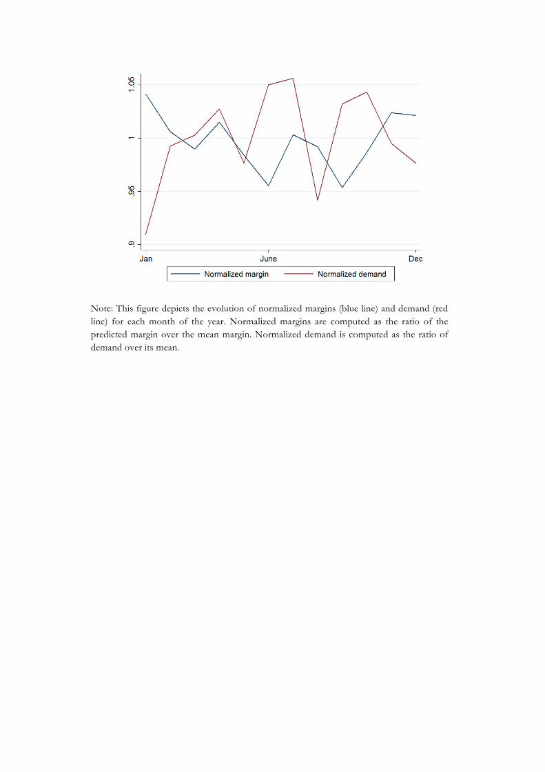
Note: This figure depicts the evolution of normalized margins (blue line) and demand (red line) for each month of the year. Normalized margins are computed as the ratio of the predicted margin over the mean margin. Normalized demand is computed as the ratio of demand over its mean.

Table 1: Estimations of Equations (1) and (2) and Alternative Specifications for Diesel

(1) (2) (3) (4) Variables Margins Margins Margins Margins EDEMANDt+1 -0.648*** -0.389** -0.519*** -0.527*** (0.225) (0.163) (0.177) (0.170) DEMANDt -0.358*** -0.284*** -0.609*** -0.359*** (0.118) (0.104) (0.147) (0.104) EMCt+1 -0.229*** 0.0393 -0.00206 -0.0174 (0.055) (0.145) (0.0592) (0.0778) MCt 0.205*** 0.0577 0.0691 (0.052) (0.0521) (0.0602) MCt-1 0.164* (0.0871) CRUDEt-1 -0.182** (0.0847) �MC+t -0.219 -0.180*** (0.185) (0.0613) �MC-t -0.221** -0.288*** (0.104) (0.0578) �MC+t-1 -0.0926 0.0640 (0.118) (0.0555) �MC-t-1 -0.0124 0.000583 (0.0570) (0.0488) �CRUDE+t 0.0562 (0.100) �CRUDE-t -0.0240 (0.137) �CRUDE+t-1 0.160 (0.112) �CRUDE-t-1 0.0545 (0.0908) �DEMANDt 0.219** (0.0975) � MCt -0.231*** (0.0396) �DEMAND+t 0.674*** (0.176) �DEMAND-t 0.351** (0.156) �DEMAND+t-1 -0.784*** (0.189) �DEMAND-t-1 -0.815*** (0.202) Constant 23.14*** 16.03*** 19.47*** 24.81*** (2.490) (2.396) (2.256) (2.832) Observations 282 282 282 282 R-squared 0.860 0.897 0.892 0.901

Note: This table reports how margins are impacted by marginal costs and demand. All of the models are OLS specifications. All of the regressions include year fixed effects. Robust standard errors are presented in parentheses with *** p<0.01, ** p<0.05 and * p<0.1.

Table 2: Estimations of Equations (1) and (2) and Alternative Specifications for Premium

(1) (2) (3) (4) Variables Margins Margins Margins Margins EDEMANDt+1 0.126 -0.200 0.0957 -0.0727 (0.472) (0.414) (0.401) (0.423) DEMANDt -0.887*** -0.958*** -1.184*** -1.05*** (0.284) (0.268) (0.350) (0.358) EMCt+1 -0.242*** 0.403** 0.157 0.321* (0.0563) (0.158) (0.108) (0.182) MCt 0.240*** -0.0373 -0.155 (0.0530) (0.0859) (0.130) MCt-1 -0.186* (0.104) CRUDEt-1 -0.0564 (0.120) �MC+t -0.493** -0.249*** (0.191) (0.0795) �MC-t -0.622*** -0.424*** (0.223) (0.132) �MC+t-1 -0.0182 0.0572 (0.110) (0.0775) �MC-t-1 -0.0898 -0.0875 (0.118) (0.0919) �CRUDE+t 0.0755 (0.162) �CRUDE-t -0.176 (0.130) �CRUDE+t-1 0.214 (0.228) �CRUDE-t-1 -0.0344 (0.161) �DEMANDt 0.367 (0.338) � MCt -0.283*** (0.0683) �DEMAND+t 0.284 (0.630) �DEMAND-t 0.0445 (0.592) �DEMAND+t-1 0.00480 (0.510) �DEMAND-t-1 0.109 (0.651) Constant 17.90*** 3.348 10.50*** 6.847 (1.440) (4.227) (2.679) (5.055) Observations 280 280 280 280 R-squared 0.765 0.802 0.794 0.797

Note: This table reports how margins are impacted by marginal costs and demand. All of the models are OLS specifications. All of the regressions include year fixed effects. Robust standard errors are presented in parentheses with *** p<0.01, ** p<0.05 and * p<0.1.

The results of our study are interesting for at least two reasons. First, they shed light on the determinants of margins in this oligopoly. However, whether margins reveal collusive or non-collusive behavior remains an open question. Margins tend to decrease when next-period demand increases, as predicted by the non-collusive models. However, marginal costs have a negative impact on margins, as predicted by the collusive models. Second, the results suggest that firm behavior does not follow the single-period Nash equilibrium solution but is characterized by both anti-cooperative and pro-cooperative movements. Our results show that on average, gasoline retailers do not act as the tight oligopoly that we might imagine, even though they tend to increase their overall margins.

5. Conclusion

Using a panel on retail fuel margins in France over more than twenty years, we found mitigated evidence of collusive behavior in the retail gasoline industry. On the one hand, we find lower margins when demand is expected to increase in the next period, a prediction that is standard to the non-cooperative models. On the other hand, we find evidence for tacit collusion as margins respond to input cost changes in the manner that the tacit collusion models predict: margins decline when the expected marginal costs increase.

The results are not surprising because the retail gasoline industry is not the tight oligopoly that has been supposed in some formal models. For example, switching costs are an important factor to be considered. However, the large inelasticity of demand for gasoline makes the industry a good candidate for setting prices that reflect a high level of market power. Our results are useful for studying competition at the industry level.

References

Borenstein, S. and A. Shepard, “Dynamic Pricing in Retail Gasoline Markets”, The Rand Journal of Economics, 27(3), 429-451, 1996.

Klemperer, P., “The Competitiveness of Markets with Switching Costs”, The Rand Journal of Economics, 18(1), 137-150, 1987.

Haltiwanger J. and J.J. Harrington, “The Impact of Cyclical Demand Movement on Collusive Behavior”, The Rand Journal of Economics, 22(2), 89-116, 1991.

Houde, J-F., “Gasoline Markets” in The New Palgrave Dictionary of Economics, edited by S. N. Durlauf and L.E. Blume, Online Edition, 2011.

Maskin, E. and J. Tirole, “A Theory of Dynamic Oligopoly, ii: Price Competition, Kinked Demand Curves, and Edgeworth Cycles”, Econometrica, 56(3), 571-599, 1988.

Noel, M.D., “Edgeworth Price Cycles” in The New Palgrave Dictionary of Economics, edited by S. N. Durlauf and L.E. Blume, Online Edition, 2011.

Rotemberg, J.J. and G. Saloner, “A Supergame-Theoretic Model of Price Wars During Booms”, The American Economic Review, 76(3), 390-407, 1986.

Appendix

A.1. Equations Used to Estimate Expected Demand and Expected Marginal Costs

We compute simple econometric models for expected demand and marginal costs. To construct the expected demand, we assume that the industry builds its expectations for the evolution of consumption based on the current and past levels of demand. The model is then:

Demandt = �0 + �1 Demandt-1 + �2 Pricet-1 + � + � t

where Demandt is consumption for a given month t, Pricet-1 is the retail price paid by consumers net of taxes at t-1 and � includes the month and year fixed effects. The fitted values of this equation are then used to compute the expected demand.

Computing the expected marginal costs allows us to use more of the available information and to use a full lag structure. The following model is estimated:

MCt = �0 + �1 MCt-1 + �2 � MC+t-1 + �3 � MC-

t-1 + �4 � MC+t-2 + �5 � MC-

t-2 + �+ � t

where MCt is the marginal cost for a given month t, � MC+t-1 is the interaction term between the

variation of marginal costs and a dummy that equals 1 if the marginal costs have increased between t-1 and the previous period, � MC-

t-1 is the interaction term between the variation of marginal costs and a dummy that equals 1 if the marginal costs have decreased between t-1 and the previous period and � includes the month and year fixed effects. The expected marginal costs for the next period for a given month t are the fitted values from estimating this equation. Note that when we consider Rotterdam prices as the marginal costs, we also include the t-1 and t-2 interaction terms for crude oil prices and the lagged crude oil price. Such a specification is analogous to that used by Borenstein and Shepard [1996]. The results are reported in Table A.1 for demand and Table A.2 for marginal costs.

Table A.1: Estimates of Demand, Diesel and Premium

(1) (2) Variables Demand,

Diesel Demand, Premium

Demandt-1 -0.287*** -0.062 (0.0669) (0.0897) Pricet-1 0.435 -2.328*** (1.320) (0.573) Constant 889.8*** 1690.99*** (87.85) (158.611) Observations 368 279 R-squared 0.990 0.984

Note: This table reports how demand responds to past evolutions in marginal costs. All of the models are OLS specifications. Model (1) uses data on diesel, and Model (2) uses data on premium gasoline. All of the regressions include month and year fixed effects. Robust standard errors are presented in parentheses with *** p<0.01, ** p<0.05 and * p<0.1.

Table A.2: Estimates of Marginal Costs, Diesel and Premium

(1) (2) (3) Variables Rotterdam Crude oil Crude oil Rotterdamt-1 0.485*** 0.729*** (0.167) (0.062) Crudet-1 0.327* 0.675*** 0.675*** (0.187) (0.0682) (0.0682) � Crude+t-1 -0.564** -0.063 -0.161 (0.236) (0.142) (0.189) � Crude+t-2 -0.262 -0.208 0.0711 (0.304) (0.1534) (0.164) � Crude-t-1 0.418 0.067 0.344** (0.270) (0.169) (0.154) � Crude-t-2 0.327 0.159 0.224 (0.219) (0.131) (0.158) � Rotterdam+t-1 0.760*** 0.202 (0.238) (0.157) � Rotterdam+t-2 0.421 -0.065 (0.281) (0.162) � Rotterdam-t-1 -0.155 0.581*** (0.198) (0.159) � Rotterdam-t-2 -0.0539 0.101 (0.135) (0.122) Constant 3.968*** 6.159*** 7.378*** (0.930) (1.383) (1.498) Observations 366 366 366 R-squared 0.989 0.985 0.981

Note: This table reports how marginal costs respond to past evolutions in demand. All of the models are OLS specifications. Model (1) uses data on diesel, and Model (2) uses data on premium gasoline. All of the regressions include month and year fixed effects. Robust standard errors are presented in parentheses with *** p<0.01, ** p<0.05 and * p<0.1.