Embed Size (px)
Citation preview
Aalborg Universitet
Experimental Set-up and Full-scale measurements in the ‘Cube'
Kalyanova, Olena; Heiselberg, Per
Publication date:2008
Document VersionPublisher's PDF, also known as Version of record
Link to publication from Aalborg University
Citation for published version (APA):Kalyanova, O., & Heiselberg, P. (2008). Experimental Set-up and Full-scale measurements in the ‘Cube'.Department of Civil Engineering, Aalborg University. DCE Technical reports No. 34
General rightsCopyright and moral rights for the publications made accessible in the public portal are retained by the authors and/or other copyright ownersand it is a condition of accessing publications that users recognise and abide by the legal requirements associated with these rights.
- Users may download and print one copy of any publication from the public portal for the purpose of private study or research. - You may not further distribute the material or use it for any profit-making activity or commercial gain - You may freely distribute the URL identifying the publication in the public portal -
Take down policyIf you believe that this document breaches copyright please contact us at [email protected] providing details, and we will remove access tothe work immediately and investigate your claim.
Downloaded from vbn.aau.dk on: February 12, 2022
Department of Civil Engineering
ISSN 1901-726X DCE Technical Report No. 034
Experimental Set-up and Full-scale measurements in ‘the Cube’
Technical Report
O. Kalyanova P. Heiselberg
2
DCE Technical Report No. 034
Experimental Set-up and Full-scale measurements in the ‘Cube’
by
O. Kalyanova P. Heiselberg
May 2008
© Aalborg University
Aalborg University Department of Civil Engineering
Indoor Environmental Engineering Research Group
3
Scientific Publications at the Department of Civil Engineering Technical Reports are published for timely dissemination of research results and scientific work carried out at the Department of Civil Engineering (DCE) at Aalborg University. This medium allows publication of more detailed explanations and results than typically allowed in scientific journals. Technical Memoranda are produced to enable the preliminary dissemination of scientific work by the personnel of the DCE where such release is deemed to be appropriate. Documents of this kind may be incomplete or temporary versions of papers—or part of continuing work. This should be kept in mind when references are given to publications of this kind. Contract Reports are produced to report scientific work carried out under contract. Publications of this kind contain confidential matter and are reserved for the sponsors and the DCE. Therefore, Contract Reports are generally not available for public circulation. Lecture Notes contain material produced by the lecturers at the DCE for educational purposes. This may be scientific notes, lecture books, example problems or manuals for laboratory work, or computer programs developed at the DCE. Theses are monograms or collections of papers published to report the scientific work carried out at the DCE to obtain a degree as either PhD or Doctor of Technology. The thesis is publicly available after the defence of the degree. Latest News is published to enable rapid communication of information about scientific work carried out at the DCE. This includes the status of research projects, developments in the laboratories, information about collaborative work and recent research results.
Published 2008 by Aalborg University Department of Civil Engineering Sohngaardsholmsvej 57, DK-9000 Aalborg, Denmark Printed in Denmark at Aalborg University ISSN 1901-726X DCE Technical Report No. 034

4
5
INDEX
11.. AN OUTDOOR TEST FACILITY ‘THE CUBE’.............................................................6 1.1 FOREWORD.......................................................................................................................6 1.2 GEOGRAPHY AND SITE LOCATION ....................................................................................6 1.3 ‘THE CUBE’, THE MAIN PRINCIPLES OF OPERATION........................................................7 1.4 GEOMETRY AND CONSTRUCTIONS OF ‘THE CUBE’...........................................................9 1.5 GROUND REFLECTION ....................................................................................................12 1.6 OPTICAL PROPERTIES OF THE SURFACES IN THE TEST FACILITY ....................................13
22.. PRELIMINARY EXPERIMENTS ...................................................................................14 2.1 “CALIBRATION” OF THE TEST FACILITY .........................................................................14
2.1.1 Tightness of ‘the Cube’ .........................................................................................14 2.1.2 Transmission heat losses of ‘the Cube’ ................................................................15
2.2 MEASUREMENT TECHNIQUES.........................................................................................17 2.2.1 Measurements of the air temperature under the direct solar irradiation............17
2.2.1.1 METHODS ..................................................................................................................... 18 2.2.1.2 RESULTS ....................................................................................................................... 19
2.2.2 Measurements of the air speed with the hot-sphere anemometer under the direct solar irradiation.....................................................................................................................21
2.2.2.1 Testing the dynamic properties of the hot-sphere anemometers ................................... 22 2.2.2.2 Testing of the hot-sphere performance when exposed to the solar radiation ................ 22 2.2.2.3 Testing of the hot-spheres for measurements of the flow direction .............................. 24 2.2.2.4 Summary ......................................................................................................................... 26
2.2.3 Calibration of openings.........................................................................................26 2.2.3.1 The discharge coefficient................................................................................................ 28
33.. THE FULL-SCALE MEASUREMENTS.........................................................................31 3.1 MODES OF THE DSF PERFORMANCE IN THE EXPERIMENTS............................................31 3.2 THE EXPERIMENTAL SET-UP ..........................................................................................32
3.2.1 Temperature ..........................................................................................................32 3.2.1.1 Temperature measurements in the Experiment room .................................................... 33 3.2.1.2 Temperature measurements in the DSF ......................................................................... 34 3.2.1.3 Measurement of inlet and outlet air temperature ........................................................... 37
3.2.2 Air flow rate in the DSF cavity .............................................................................37 3.2.2.1 Experimental setup ......................................................................................................... 39
3.2.3 Solar radiation.......................................................................................................42 3.2.4 Wind velocity profile .............................................................................................44 3.2.5 Air humidity ...........................................................................................................46 3.2.6 Climate data from the Danish Meteorological Institute (DMI) ...........................46 3.2.7 Power loads to the experiment room ....................................................................46
3.2.7.1 Cooling load.................................................................................................................... 46 3.2.7.2 Heating load.................................................................................................................... 47
3.3 EXPERIMENTAL DATA TREATMENT................................................................................47 APPENDIX.....................................................................................................................................1
Physical properties of the constructions .................................................................................3 Walls’ properties................................................................................................................................. 3 Windows’ properties........................................................................................................................... 4
Optical properties of the surfaces in the test facility ..............................................................5

6
11.. AN OUTDOOR TEST FACILITY ‘THE CUBE’
1.1 FOREWORD
‘The Cube’ is an outdoor test facility located at the main campus of Aalborg University. It has been built in the fall of 2005 with the purpose of detailed investigations of the DSF performance, development of the empirical test cases for validation and further improvements of various building simulation software for the modelling of buildings with double skin facades in the frame of IEA ECBCS ANNEX 43/SHC Task 34, Subtask E- Double Skin Facade. The test facility is designed to be flexible for a choice of the DSF operational modes, natural or mechanical flow conditions, different types of shading devices etc. Moreover, the superior control of the thermal conditions in the room adjacent to the DSF and the opening control allow to investigate the DSF both as a part of complete ventilation system and as a separate element of building construction. The test facility is equipped to allow measurements of any power supplied to the experimental zone in order to maintain the necessary thermal conditions. An accuracy of these measurements is justified by the quality of the facility construction: ‘the Cube’ is very well insulated and tight.
1.2 GEOGRAPHY AND SITE LOCATION
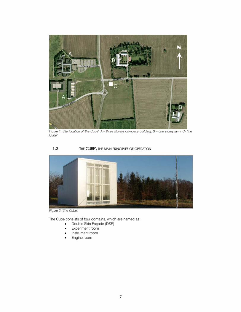
The experimental test facility ‘the Cube’ is located in the suburban area, in a neighbourhood of a few company buildings and farms (Figure 1). Windows of the double skin façade face to the South. The following coordinates define its’ geographical location: Time zone +1 hr MGT Degrees of longitude 9.93 East Degrees of latitude 57.05 North Altitude 19 m Table 1.Geographical and site parameters of ‘the Cube’.
7
Figure 1. Site location of 'the Cube'. A – three storeys company building, B – one storey farm, C- ‘the Cube’.
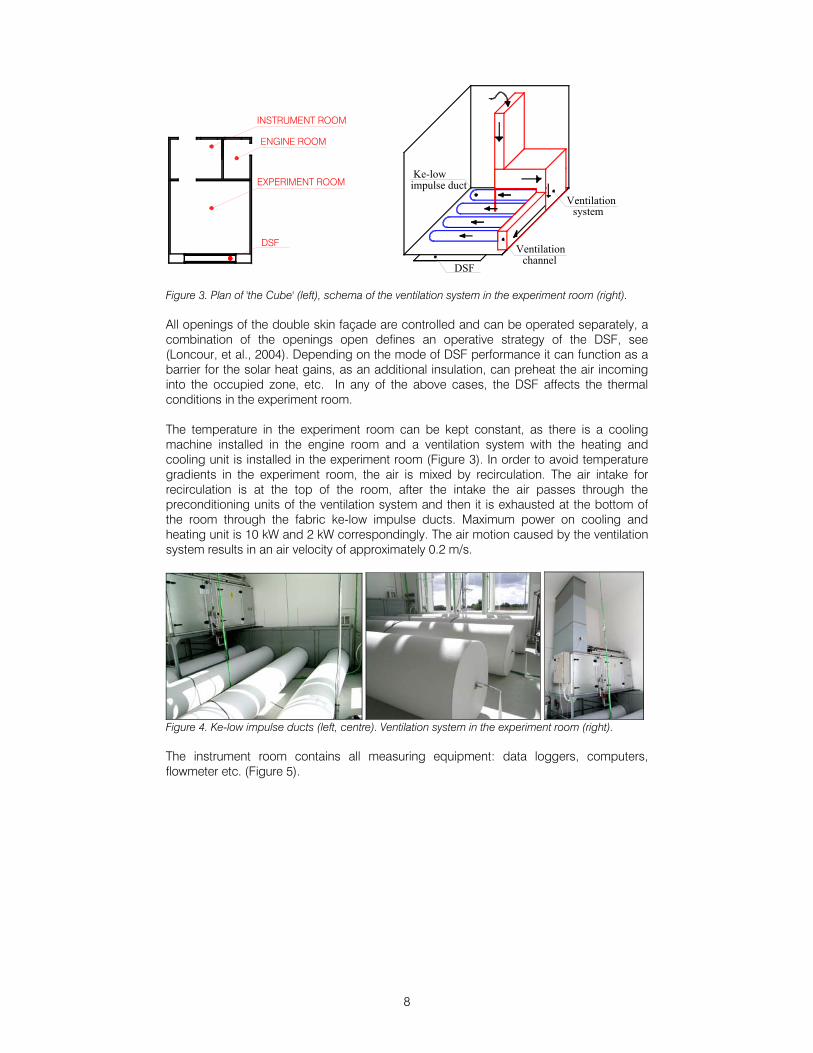
1.3 ‘THE CUBE’, THE MAIN PRINCIPLES OF OPERATION
Figure 2. 'The Cube'. The Cube consists of four domains, which are named as:
• Double Skin Façade (DSF) • Experiment room • Instrument room • Engine room
A
A
B
B
C
N
8
DSF
ENGINE ROOM
INSTRUMENT ROOM
EXPERIMENT ROOM
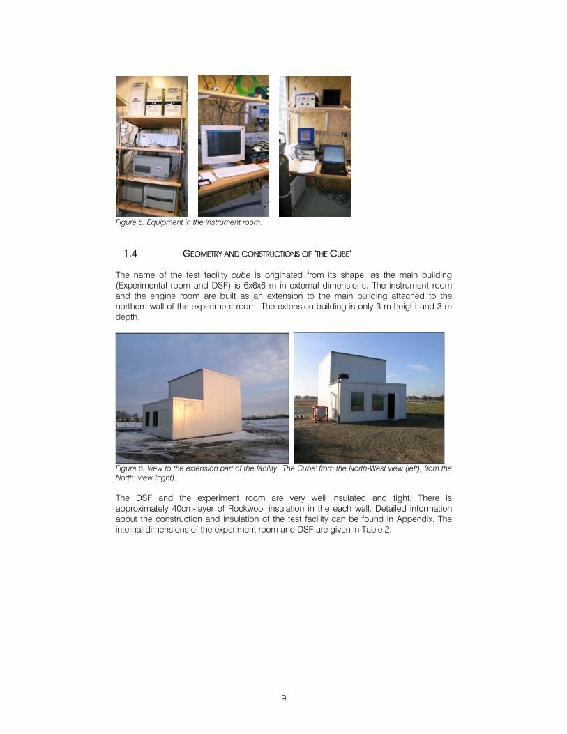
Figure 3. Plan of 'the Cube' (left), schema of the ventilation system in the experiment room (right). All openings of the double skin façade are controlled and can be operated separately, a combination of the openings open defines an operative strategy of the DSF, see (Loncour, et al., 2004). Depending on the mode of DSF performance it can function as a barrier for the solar heat gains, as an additional insulation, can preheat the air incoming into the occupied zone, etc. In any of the above cases, the DSF affects the thermal conditions in the experiment room. The temperature in the experiment room can be kept constant, as there is a cooling machine installed in the engine room and a ventilation system with the heating and cooling unit is installed in the experiment room (Figure 3). In order to avoid temperature gradients in the experiment room, the air is mixed by recirculation. The air intake for recirculation is at the top of the room, after the intake the air passes through the preconditioning units of the ventilation system and then it is exhausted at the bottom of the room through the fabric ke-low impulse ducts. Maximum power on cooling and heating unit is 10 kW and 2 kW correspondingly. The air motion caused by the ventilation system results in an air velocity of approximately 0.2 m/s.
Figure 4. Ke-low impulse ducts (left, centre). Ventilation system in the experiment room (right). The instrument room contains all measuring equipment: data loggers, computers, flowmeter etc. (Figure 5).
DSF
Ventilationchannel
Ventilationsystem
Ke-low impulse duct
9
Figure 5. Equipment in the instrument room.
1.4 GEOMETRY AND CONSTRUCTIONS OF ‘THE CUBE’
The name of the test facility cube is originated from its shape, as the main building (Experimental room and DSF) is 6x6x6 m in external dimensions. The instrument room and the engine room are built as an extension to the main building attached to the northern wall of the experiment room. The extension building is only 3 m height and 3 m depth.
Figure 6. View to the extension part of the facility. 'The Cube' from the North-West view (left), from the North view (right). The DSF and the experiment room are very well insulated and tight. There is approximately 40cm-layer of Rockwool insulation in the each wall. Detailed information about the construction and insulation of the test facility can be found in Appendix. The internal dimensions of the experiment room and DSF are given in Table 2.
10
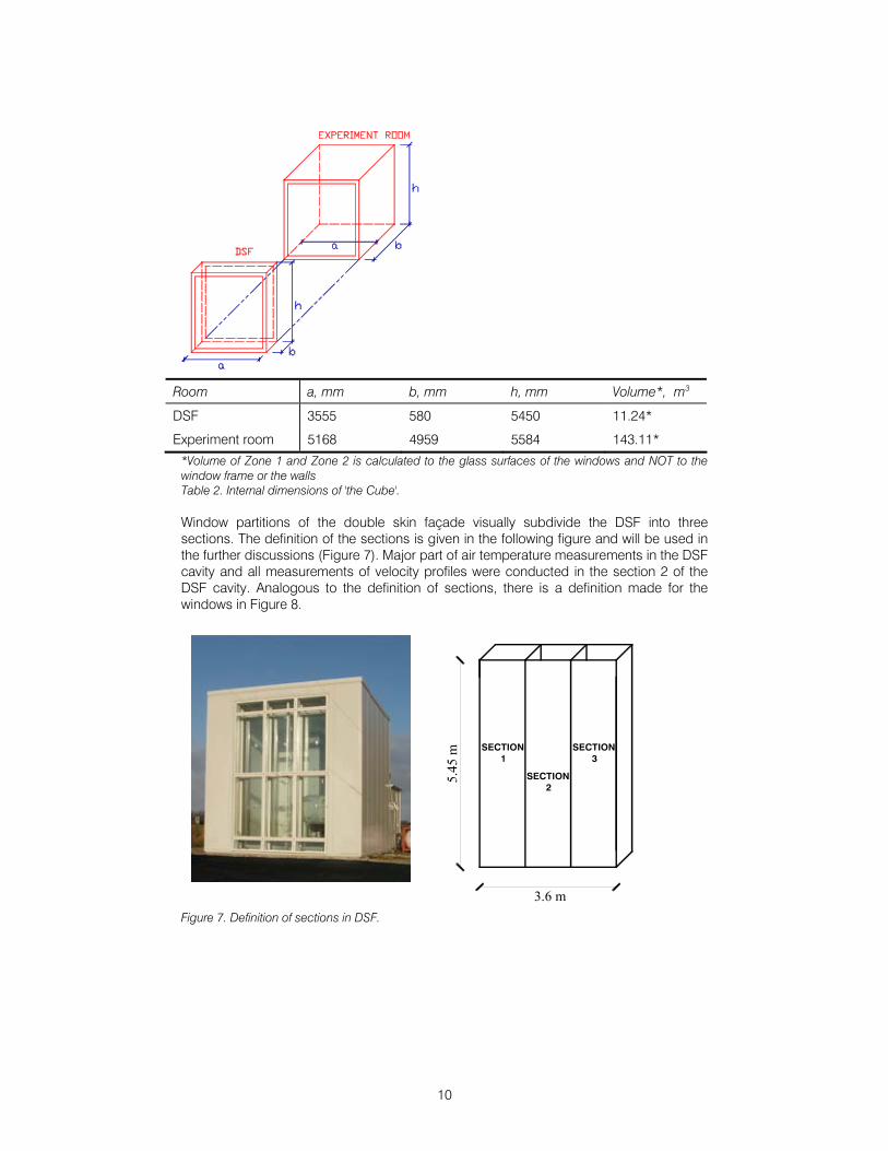
*Volume of Zone 1 and Zone 2 is calculated to the glass surfaces of the windows and NOT to the window frame or the walls Table 2. Internal dimensions of 'the Cube'. Window partitions of the double skin façade visually subdivide the DSF into three sections. The definition of the sections is given in the following figure and will be used in the further discussions (Figure 7). Major part of air temperature measurements in the DSF cavity and all measurements of velocity profiles were conducted in the section 2 of the DSF cavity. Analogous to the definition of sections, there is a definition made for the windows in Figure 8.
3.6 m
5.45
m SECTION 1
SECTION 2
SECTION 3
Figure 7. Definition of sections in DSF.
Room a, mm b, mm h, mm Volume*, m3
DSF 3555 580 5450 11.24*
Experiment room 5168 4959 5584 143.11*
11
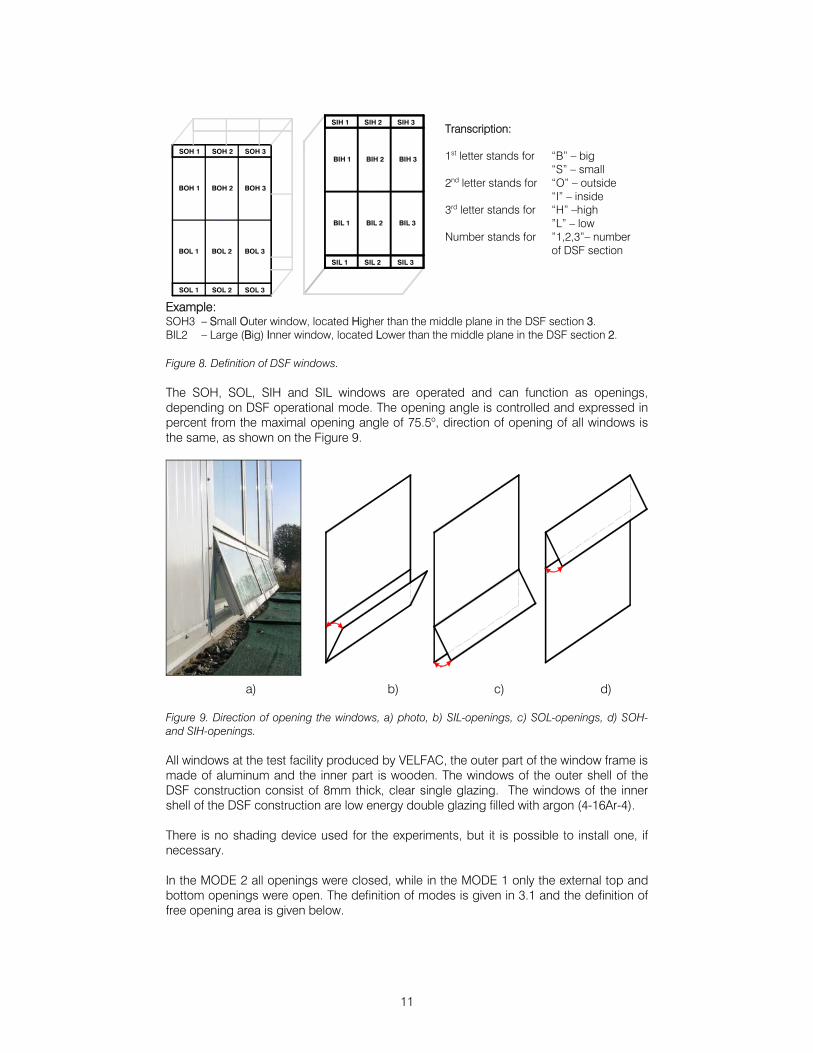
SOL 1 SOL 2 SOL 3
SOH 1 SOH 2 SOH 3
BOH 1 BOH 2 BOH 3
BOL 1 BOL 2 BOL 3
SIL 1 SIL 2 SIL 3
SIH 1 SIH 2 SIH 3
BIH 1 BIH 2 BIH 3
BIL 1 BIL 2 BIL 3
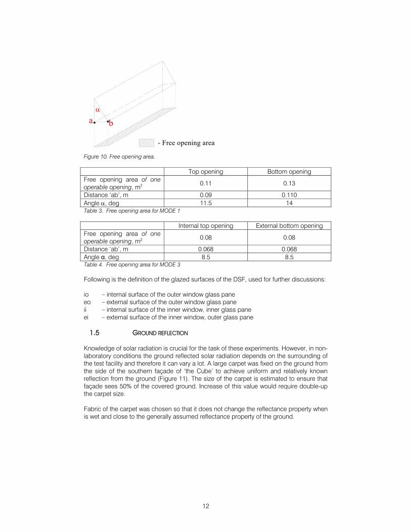
Example: SOH3 – Small Outer window, located Higher than the middle plane in the DSF section 3. BIL2 – Large (Big) Inner window, located Lower than the middle plane in the DSF section 2. Figure 8. Definition of DSF windows. The SOH, SOL, SIH and SIL windows are operated and can function as openings, depending on DSF operational mode. The opening angle is controlled and expressed in percent from the maximal opening angle of 75.5o, direction of opening of all windows is the same, as shown on the Figure 9.
Figure 9. Direction of opening the windows, a) photo, b) SIL-openings, c) SOL-openings, d) SOH- and SIH-openings. All windows at the test facility produced by VELFAC, the outer part of the window frame is made of aluminum and the inner part is wooden. The windows of the outer shell of the DSF construction consist of 8mm thick, clear single glazing. The windows of the inner shell of the DSF construction are low energy double glazing filled with argon (4-16Ar-4). There is no shading device used for the experiments, but it is possible to install one, if necessary. In the MODE 2 all openings were closed, while in the MODE 1 only the external top and bottom openings were open. The definition of modes is given in 3.1 and the definition of free opening area is given below.
Transcription: 1st letter stands for “B” – big “S” – small 2nd letter stands for “O” – outside “I” – inside 3rd letter stands for “H” –high ”L” – low Number stands for ”1,2,3”– number of DSF section
a) b) c) d)
12
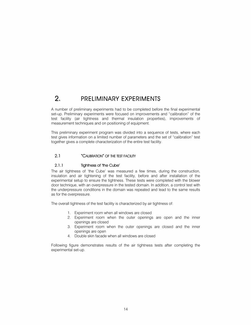
- Free opening area
a bα
Figure 10. Free opening area. Top opening Bottom opening Free opening area of one operable opening, m2 0.11 0.13
Distance ‘ab’, m 0.09 0.110 Angle α, deg 11.5 14 Table 3. Free opening area for MODE 1 Internal top opening External bottom opening Free opening area of one operable opening, m2 0.08 0.08
Distance ‘ab’, m 0.068 0.068 Angle α, deg 8.5 8.5 Table 4. Free opening area for MODE 3 Following is the definition of the glazed surfaces of the DSF, used for further discussions: io – internal surface of the outer window glass pane eo – external surface of the outer window glass pane ii – internal surface of the inner window, inner glass pane ei – external surface of the inner window, outer glass pane
1.5 GROUND REFLECTION
Knowledge of solar radiation is crucial for the task of these experiments. However, in non-laboratory conditions the ground reflected solar radiation depends on the surrounding of the test facility and therefore it can vary a lot. A large carpet was fixed on the ground from the side of the southern façade of ‘the Cube’ to achieve uniform and relatively known reflection from the ground (Figure 11). The size of the carpet is estimated to ensure that façade sees 50% of the covered ground. Increase of this value would require double-up the carpet size. Fabric of the carpet was chosen so that it does not change the reflectance property when is wet and close to the generally assumed reflectance property of the ground.

13
Figure 11. Illustration of the ground carpet in front of ‘the Cube’.
1.6 OPTICAL PROPERTIES OF THE SURFACES IN THE TEST FACILITY
Absorption, reflection and transmission properties of the most exposed to solar radiation surfaces in the DSF and experiment room were tested at the EMPA Materials Science & Technology Laboratory. Available information about the optical properties of surfaces can be found in Appendix as a function of the wave length. The spectral data in the wave length interval 250-2500nm is given there for the following surfaces:
• Glazing • Ceiling and wall surface finishing in the DSF • Ceiling and wall surface finishing in the experiment room • Carpet in front of ‘the Cube’
14
22.. PRELIMINARY EXPERIMENTS
A number of preliminary experiments had to be completed before the final experimental set-up. Preliminary experiments were focused on improvements and “calibration” of the test facility (air tightness and thermal insulation properties), improvements of measurement techniques and on positioning of equipment. This preliminary experiment program was divided into a sequence of tests, where each test gives information on a limited number of parameters and the set of “calibration” test together gives a complete characterization of the entire test facility.
2.1 “CALIBRATION” OF THE TEST FACILITY
2.1.1 Tightness of ‘the Cube’ The air tightness of ‘the Cube’ was measured a few times, during the construction, insulation and air tightening of the test facility, before and after installation of the experimental setup to ensure the tightness. These tests were completed with the blower door technique, with an overpressure in the tested domain. In addition, a control test with the underpressure conditions in the domain was repeated and lead to the same results as for the overpressure. The overall tightness of the test facility is characterized by air tightness of:
1. Experiment room when all windows are closed 2. Experiment room when the outer openings are open and the inner
openings are closed 3. Experiment room when the outer openings are closed and the inner
openings are open 4. Double skin facade when all windows are closed
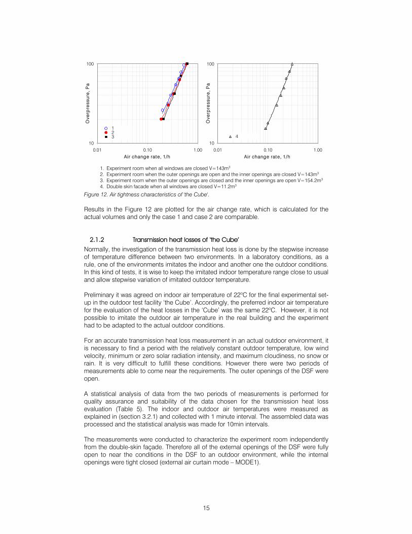
Following figure demonstrates results of the air tightness tests after completing the experimental set-up.
15
10
100
0.01 0.10 1.00Air change rate, 1/h
Ove
rpre
ssu
re,
Pa
123
10
100
0.01 0.10 1.00Air change rate, 1/h
Ove
rpre
ssu
re,
Pa
4
Figure 12. Air tightness characteristics of 'the Cube'. Results in the Figure 12 are plotted for the air change rate, which is calculated for the actual volumes and only the case 1 and case 2 are comparable.
2.1.2 Transmission heat losses of ‘the Cube’ Normally, the investigation of the transmission heat loss is done by the stepwise increase of temperature difference between two environments. In a laboratory conditions, as a rule, one of the environments imitates the indoor and another one the outdoor conditions. In this kind of tests, it is wise to keep the imitated indoor temperature range close to usual and allow stepwise variation of imitated outdoor temperature. Preliminary it was agreed on indoor air temperature of 22oC for the final experimental set-up in the outdoor test facility ‘the Cube’. Accordingly, the preferred indoor air temperature for the evaluation of the heat losses in the ‘Cube’ was the same 22oC. However, it is not possible to imitate the outdoor air temperature in the real building and the experiment had to be adapted to the actual outdoor conditions. For an accurate transmission heat loss measurement in an actual outdoor environment, it is necessary to find a period with the relatively constant outdoor temperature, low wind velocity, minimum or zero solar radiation intensity, and maximum cloudiness, no snow or rain. It is very difficult to fulfill these conditions. However there were two periods of measurements able to come near the requirements. The outer openings of the DSF were open. A statistical analysis of data from the two periods of measurements is performed for quality assurance and suitability of the data chosen for the transmission heat loss evaluation (Table 5). The indoor and outdoor air temperatures were measured as explained in (section 3.2.1) and collected with 1 minute interval. The assembled data was processed and the statistical analysis was made for 10min intervals. The measurements were conducted to characterize the experiment room independently from the double-skin façade. Therefore all of the external openings of the DSF were fully open to near the conditions in the DSF to an outdoor environment, while the internal openings were tight closed (external air curtain mode – MODE1).
1. Experiment room when all windows are closed V=143m3 2. Experiment room when the outer openings are open and the inner openings are closed V=143m3 3. Experiment room when the outer openings are closed and the inner openings are open V=154.2m3 4. Double skin facade when all windows are closed V=11.2m3
16
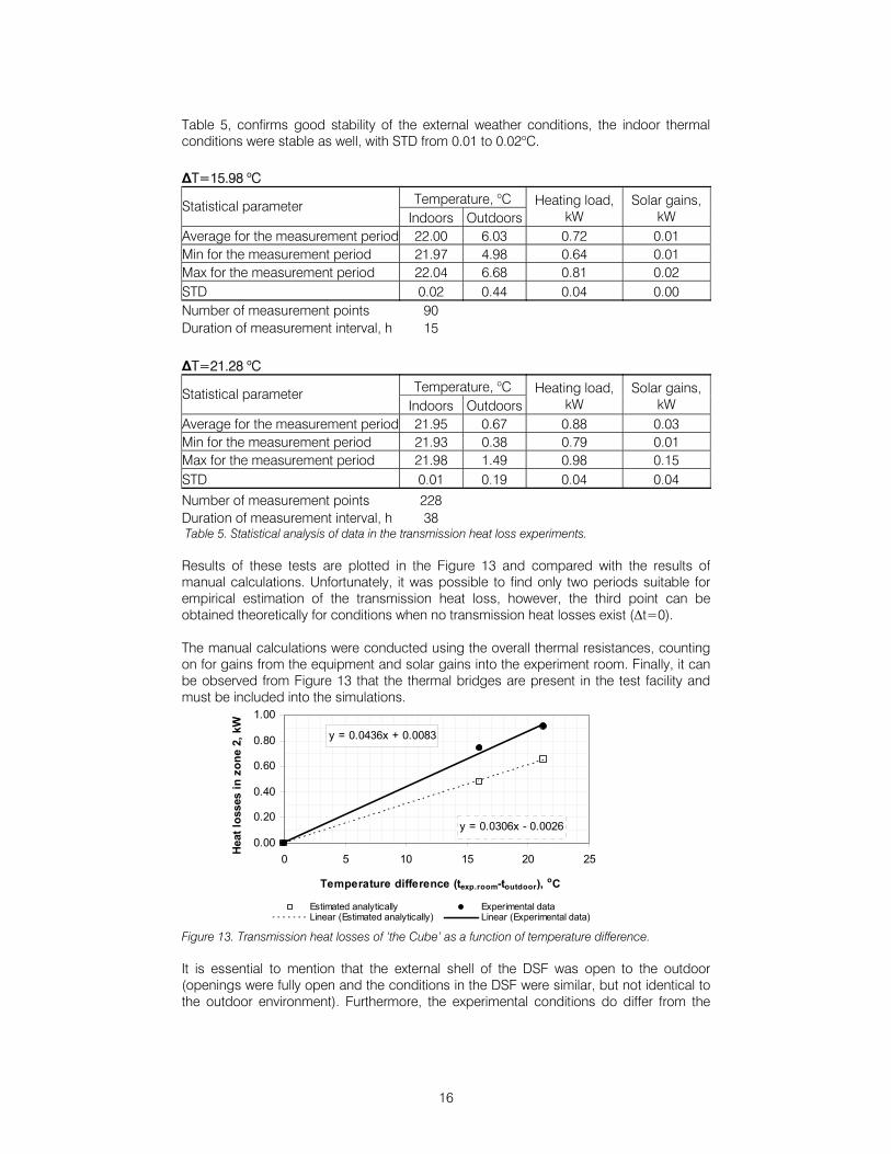
Table 5, confirms good stability of the external weather conditions, the indoor thermal conditions were stable as well, with STD from 0.01 to 0.02oC. ΔT=15.98 oC
Temperature, oC Statistical parameter Indoors Outdoors
Heating load, kW
Solar gains, kW
Average for the measurement period 22.00 6.03 0.72 0.01 Min for the measurement period 21.97 4.98 0.64 0.01 Max for the measurement period 22.04 6.68 0.81 0.02 STD 0.02 0.44 0.04 0.00 Number of measurement points 90 Duration of measurement interval, h 15 ΔT=21.28 oC
Temperature, oC Statistical parameter Indoors Outdoors
Heating load, kW
Solar gains, kW
Average for the measurement period 21.95 0.67 0.88 0.03 Min for the measurement period 21.93 0.38 0.79 0.01 Max for the measurement period 21.98 1.49 0.98 0.15 STD 0.01 0.19 0.04 0.04
Number of measurement points 228 Duration of measurement interval, h 38 Table 5. Statistical analysis of data in the transmission heat loss experiments. Results of these tests are plotted in the Figure 13 and compared with the results of manual calculations. Unfortunately, it was possible to find only two periods suitable for empirical estimation of the transmission heat loss, however, the third point can be obtained theoretically for conditions when no transmission heat losses exist (Δt=0). The manual calculations were conducted using the overall thermal resistances, counting on for gains from the equipment and solar gains into the experiment room. Finally, it can be observed from Figure 13 that the thermal bridges are present in the test facility and must be included into the simulations.
y = 0.0306x - 0.0026
y = 0.0436x + 0.0083
0.00
0.20
0.40
0.60
0.80
1.00
0 5 10 15 20 25
Temperature difference (texp.room-toutdoor), oC
Hea
t los
ses
in z
one
2, k
W
Estimated analytically Experimental dataLinear (Estimated analytically) Linear (Experimental data)
Figure 13. Transmission heat losses of ‘the Cube’ as a function of temperature difference. It is essential to mention that the external shell of the DSF was open to the outdoor (openings were fully open and the conditions in the DSF were similar, but not identical to the outdoor environment). Furthermore, the experimental conditions do differ from the
17
ideal situation and there is a risk of rim or snow layer on the roof of the test facility during the measurement with Δt=21.28oC.
2.2 MEASUREMENT TECHNIQUES
Since a long time ago, experiments became a common practice for a scientist. Nowadays, there is a lot of literature exists and the principles of the various measurement techniques are well developed, characterized and in most of the cases their application is already evaluated and rated. However, the situation is different when unusual experimental conditions are applied. Measurements in a real building are different from the measurement in the laboratory. One must adapt the measurement program to the outdoor conditions, to disturbances of experiments and to possible limits in a number of test sequences. Detailed measurement in a full-size building is also different from the scale-models, as it requires large amount of equipment. Besides, the reliable experimental data obtained in outdoor conditions often implies high sampling frequencies; otherwise an essential data can be lost. All of this together, results in a vast amount of data to be processed and analyzed. And, finally, measurements in a DSF building or in the DSF itself aren’t an easy matter, most of the measurement techniques are developed for the conventional buildings and can’t be directly applied in DSF, as even the air temperature can become difficult to measure accurately in the DSF cavity. On account of these concerns, a set of tests was completed to improve a quality of measurements in ‘the Cube’.
2.2.1 Measurements of the air temperature under the direct solar irradiation
The presence of the direct solar radiation is an essential element for the façade operation, but it can heavily affect measurements of air temperature and may lead to errors of high magnitude using bare thermocouples and even adopting shielding devices. An accurate air temperature measurement is crucial for prediction, evaluation and control of the dynamic performance of the façade, as a significant part of the complete ventilation system. Another distinctive element of the double skin facades is application of shading devices in the cavity in order to prevent glare and penetration of solar heat gains into the occupied zone. Depending on type of shading in the ventilated cavity, the surface of the shading device is heated up to 65oC. Location of the temperature sensor nearby the shading device may lead to serious measurement errors if the temperature sensor is unprotected. In the field of meteorology the problem of accuracy in temperature measurements was recognized over 150 years ago (Erell, et al. 2005), a screen, designed by Stevenson, is now widely used to measure air temperature in the field. Moreover, some meteorologists even suggest a standard methodology for dealing with this sort of errors. It is essential that the experts dealing with the issues of occupants’ thermal comfort consider developing of similar guidance for measurements of air temperature under the shortwave or long-wave radiation loads.
18
This section describes the experimental setup to find the best suitable technique for accurate measurements of air temperature when exposed to solar radiation.
2.2.1.1 METHODS
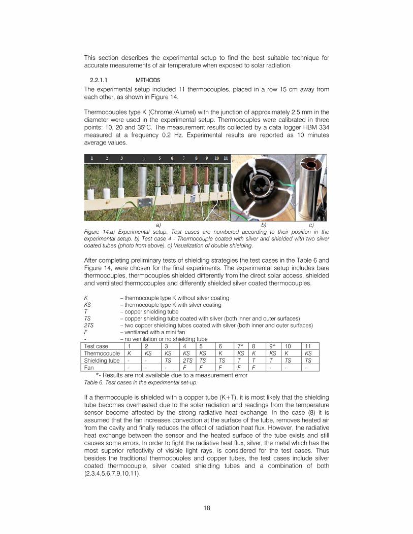
The experimental setup included 11 thermocouples, placed in a row 15 cm away from each other, as shown in Figure 14. Thermocouples type K (Chromel/Alumel) with the junction of approximately 2.5 mm in the diameter were used in the experimental setup. Thermocouples were calibrated in three points: 10, 20 and 35oC. The measurement results collected by a data logger HBM 334 measured at a frequency 0.2 Hz. Experimental results are reported as 10 minutes average values.
a) b) c) Figure 14.a) Experimental setup. Test cases are numbered according to their position in the experimental setup. b) Test case 4 - Thermocouple coated with silver and shielded with two silver coated tubes (photo from above). c) Visualization of double shielding. After completing preliminary tests of shielding strategies the test cases in the Table 6 and Figure 14, were chosen for the final experiments. The experimental setup includes bare thermocouples, thermocouples shielded differently from the direct solar access, shielded and ventilated thermocouples and differently shielded silver coated thermocouples. K – thermocouple type K without silver coating KS – thermocouple type K with silver coating T – copper shielding tube TS – copper shielding tube coated with silver (both inner and outer surfaces) 2TS – two copper shielding tubes coated with silver (both inner and outer surfaces) F – ventilated with a mini fan - – no ventilation or no shielding tube Test case 1 2 3 4 5 6 7* 8 9* 10 11 Thermocouple K KS KS KS KS K KS K KS K KS Shielding tube - - TS 2TS TS TS T T T TS TS Fan - - - F F F F F - - -
*- Results are not available due to a measurement error Table 6. Test cases in the experimental set-up. If a thermocouple is shielded with a copper tube (K+T), it is most likely that the shielding tube becomes overheated due to the solar radiation and readings from the temperature sensor become affected by the strong radiative heat exchange. In the case (8) it is assumed that the fan increases convection at the surface of the tube, removes heated air from the cavity and finally reduces the effect of radiation heat flux. However, the radiative heat exchange between the sensor and the heated surface of the tube exists and still causes some errors. In order to fight the radiative heat flux, silver, the metal which has the most superior reflectivity of visible light rays, is considered for the test cases. Thus besides the traditional thermocouples and copper tubes, the test cases include silver coated thermocouple, silver coated shielding tubes and a combination of both (2,3,4,5,6,7,9,10,11).
19
In the experimental setup shown in Figure 14 the mini fans are located at the bottom of a shielding tube and the air is sucked in the direction from the top to the bottom of the tubes. In a case of double shielding, Figure 14, one mini fan ventilates both of the cavities. Shielding tubes have the following dimensions: for the inner tube Ø25mm and length 100mm, tubes of the same dimensions were used in the other test cases. The outer tube in the test case 4: Ø60mm and length 130mm. The experimental setup was placed outdoors, in the open flat country facing south. Due to necessity to run the fans connected to the electricity the experiments were run only at the day time.
2.2.1.2 RESULTS
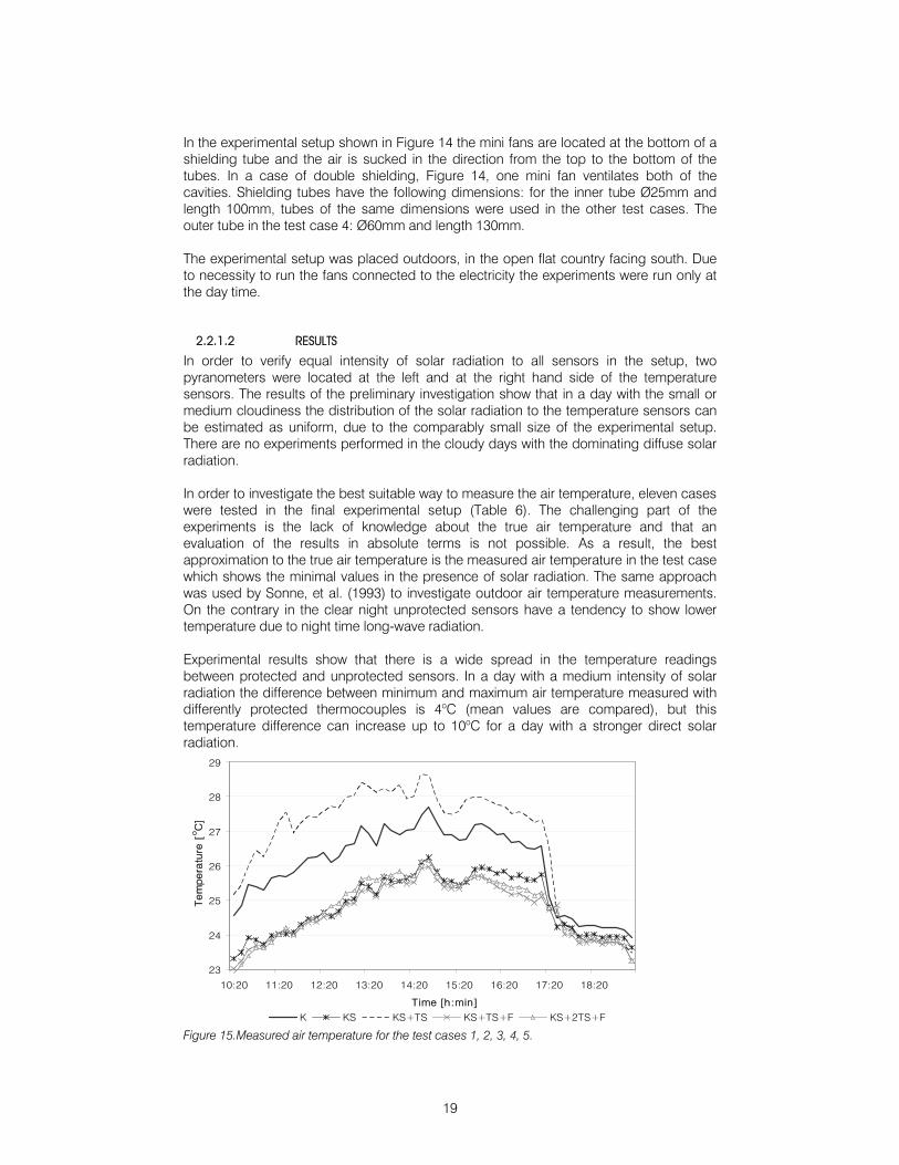
In order to verify equal intensity of solar radiation to all sensors in the setup, two pyranometers were located at the left and at the right hand side of the temperature sensors. The results of the preliminary investigation show that in a day with the small or medium cloudiness the distribution of the solar radiation to the temperature sensors can be estimated as uniform, due to the comparably small size of the experimental setup. There are no experiments performed in the cloudy days with the dominating diffuse solar radiation. In order to investigate the best suitable way to measure the air temperature, eleven cases were tested in the final experimental setup (Table 6). The challenging part of the experiments is the lack of knowledge about the true air temperature and that an evaluation of the results in absolute terms is not possible. As a result, the best approximation to the true air temperature is the measured air temperature in the test case which shows the minimal values in the presence of solar radiation. The same approach was used by Sonne, et al. (1993) to investigate outdoor air temperature measurements. On the contrary in the clear night unprotected sensors have a tendency to show lower temperature due to night time long-wave radiation. Experimental results show that there is a wide spread in the temperature readings between protected and unprotected sensors. In a day with a medium intensity of solar radiation the difference between minimum and maximum air temperature measured with differently protected thermocouples is 4oC (mean values are compared), but this temperature difference can increase up to 10oC for a day with a stronger direct solar radiation.
23
24
25
26
27
28
29
10:20 11:20 12:20 13:20 14:20 15:20 16:20 17:20 18:20
Time [h:min]
Te
mp
era
ture
[ oC
]
K KS KS+TS KS+TS+F KS+2TS+F Figure 15.Measured air temperature for the test cases 1, 2, 3, 4, 5.
20
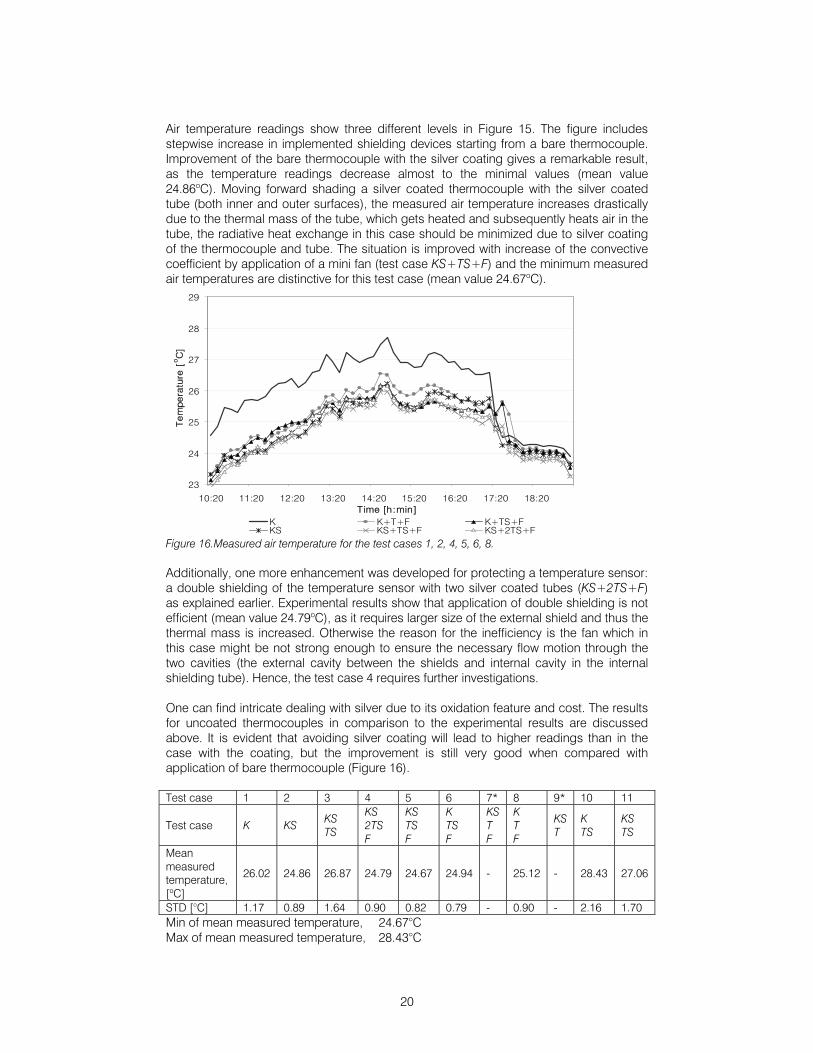
Air temperature readings show three different levels in Figure 15. The figure includes stepwise increase in implemented shielding devices starting from a bare thermocouple. Improvement of the bare thermocouple with the silver coating gives a remarkable result, as the temperature readings decrease almost to the minimal values (mean value 24.86oC). Moving forward shading a silver coated thermocouple with the silver coated tube (both inner and outer surfaces), the measured air temperature increases drastically due to the thermal mass of the tube, which gets heated and subsequently heats air in the tube, the radiative heat exchange in this case should be minimized due to silver coating of the thermocouple and tube. The situation is improved with increase of the convective coefficient by application of a mini fan (test case KS+TS+F) and the minimum measured air temperatures are distinctive for this test case (mean value 24.67oC).
23
24
25
26
27
28
29
10:20 11:20 12:20 13:20 14:20 15:20 16:20 17:20 18:20Time [h:min]
Te
mp
era
ture
[ oC
]
K K+T+F K+TS+FKS KS+TS+F KS+2TS+F
Figure 16.Measured air temperature for the test cases 1, 2, 4, 5, 6, 8. Additionally, one more enhancement was developed for protecting a temperature sensor: a double shielding of the temperature sensor with two silver coated tubes (KS+2TS+F) as explained earlier. Experimental results show that application of double shielding is not efficient (mean value 24.79oC), as it requires larger size of the external shield and thus the thermal mass is increased. Otherwise the reason for the inefficiency is the fan which in this case might be not strong enough to ensure the necessary flow motion through the two cavities (the external cavity between the shields and internal cavity in the internal shielding tube). Hence, the test case 4 requires further investigations. One can find intricate dealing with silver due to its oxidation feature and cost. The results for uncoated thermocouples in comparison to the experimental results are discussed above. It is evident that avoiding silver coating will lead to higher readings than in the case with the coating, but the improvement is still very good when compared with application of bare thermocouple (Figure 16). Test case 1 2 3 4 5 6 7* 8 9* 10 11
Test case K KS KS TS
KS 2TS F
KS TS F
K TS F
KS T F
K T F
KS T
K TS
KS TS
Mean measured temperature, [oC]
26.02 24.86 26.87 24.79 24.67 24.94 - 25.12 - 28.43 27.06
STD [°C] 1.17 0.89 1.64 0.90 0.82 0.79 - 0.90 - 2.16 1.70 Min of mean measured temperature, 24.67°C Max of mean measured temperature, 28.43°C
21
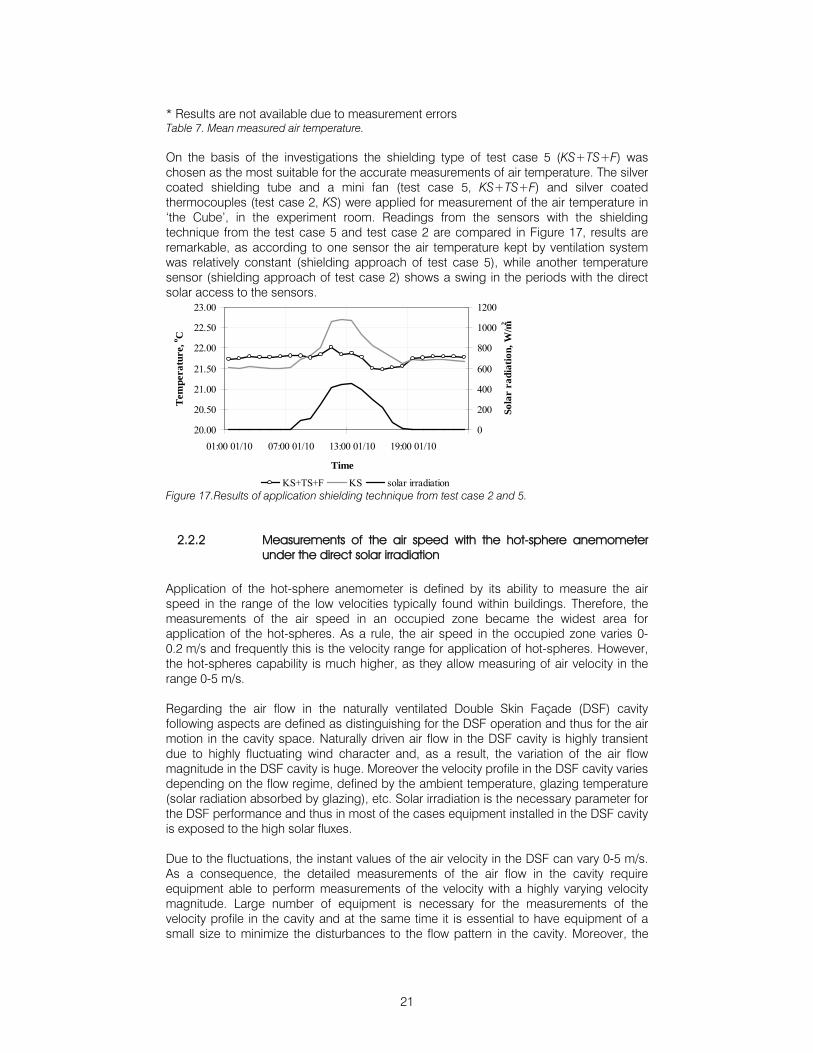
* Results are not available due to measurement errors Table 7. Mean measured air temperature. On the basis of the investigations the shielding type of test case 5 (KS+TS+F) was chosen as the most suitable for the accurate measurements of air temperature. The silver coated shielding tube and a mini fan (test case 5, KS+TS+F) and silver coated thermocouples (test case 2, KS) were applied for measurement of the air temperature in ‘the Cube’, in the experiment room. Readings from the sensors with the shielding technique from the test case 5 and test case 2 are compared in Figure 17, results are remarkable, as according to one sensor the air temperature kept by ventilation system was relatively constant (shielding approach of test case 5), while another temperature sensor (shielding approach of test case 2) shows a swing in the periods with the direct solar access to the sensors.
20.00
20.50
21.00
21.50
22.00
22.50
23.00
01:00 01/10 07:00 01/10 13:00 01/10 19:00 01/10
Time
Tem
pera
ture
, o C
0
200
400
600
800
1000
1200
Sola
r ra
diat
ion,
W/m
2
KS+TS+F KS solar irradiation Figure 17.Results of application shielding technique from test case 2 and 5.
2.2.2 Measurements of the air speed with the hot-sphere anemometer under the direct solar irradiation
Application of the hot-sphere anemometer is defined by its ability to measure the air speed in the range of the low velocities typically found within buildings. Therefore, the measurements of the air speed in an occupied zone became the widest area for application of the hot-spheres. As a rule, the air speed in the occupied zone varies 0-0.2 m/s and frequently this is the velocity range for application of hot-spheres. However, the hot-spheres capability is much higher, as they allow measuring of air velocity in the range 0-5 m/s. Regarding the air flow in the naturally ventilated Double Skin Façade (DSF) cavity following aspects are defined as distinguishing for the DSF operation and thus for the air motion in the cavity space. Naturally driven air flow in the DSF cavity is highly transient due to highly fluctuating wind character and, as a result, the variation of the air flow magnitude in the DSF cavity is huge. Moreover the velocity profile in the DSF cavity varies depending on the flow regime, defined by the ambient temperature, glazing temperature (solar radiation absorbed by glazing), etc. Solar irradiation is the necessary parameter for the DSF performance and thus in most of the cases equipment installed in the DSF cavity is exposed to the high solar fluxes. Due to the fluctuations, the instant values of the air velocity in the DSF can vary 0-5 m/s. As a consequence, the detailed measurements of the air flow in the cavity require equipment able to perform measurements of the velocity with a highly varying velocity magnitude. Large number of equipment is necessary for the measurements of the velocity profile in the cavity and at the same time it is essential to have equipment of a small size to minimize the disturbances to the flow pattern in the cavity. Moreover, the
22
equipment must be able to respond adequately to the fluctuations and also to be able to coup with the high solar loads. The described conditions in the DSF cavity are very different from the conditions in an occupied zone, but still, according to the tests described in this section the hot-sphere anemometers are an excellent choice for the measurements in the DSF cavity. It is demonstrated, how the hot sphere anemometer respond to fluctuations, to exposure to the high solar fluxes and how the hot-sphere anemometers can be used for distinguishing of the flow direction in the DSF cavity. Results of these tests were applied for measurements in ’the Cube’.
2.2.2.1 Testing the dynamic properties of the hot-sphere anemometers
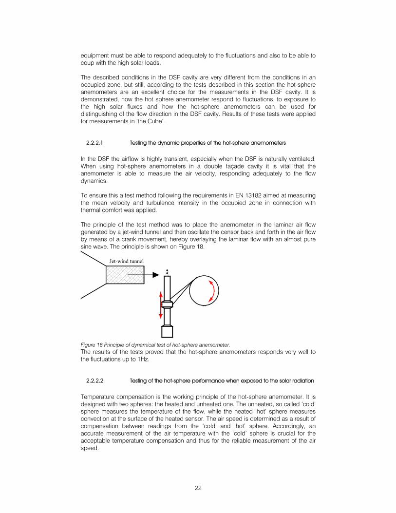
In the DSF the airflow is highly transient, especially when the DSF is naturally ventilated. When using hot-sphere anemometers in a double façade cavity it is vital that the anemometer is able to measure the air velocity, responding adequately to the flow dynamics. To ensure this a test method following the requirements in EN 13182 aimed at measuring the mean velocity and turbulence intensity in the occupied zone in connection with thermal comfort was applied. The principle of the test method was to place the anemometer in the laminar air flow generated by a jet-wind tunnel and then oscillate the censor back and forth in the air flow by means of a crank movement, hereby overlaying the laminar flow with an almost pure sine wave. The principle is shown on Figure 18.
Jet-wind tunnel
Figure 18.Principle of dynamical test of hot-sphere anemometer. The results of the tests proved that the hot-sphere anemometers responds very well to the fluctuations up to 1Hz.
2.2.2.2 Testing of the hot-sphere performance when exposed to the solar radiation
Temperature compensation is the working principle of the hot-sphere anemometer. It is designed with two spheres: the heated and unheated one. The unheated, so called ‘cold’ sphere measures the temperature of the flow, while the heated ‘hot’ sphere measures convection at the surface of the heated sensor. The air speed is determined as a result of compensation between readings from the ‘cold’ and ‘hot’ sphere. Accordingly, an accurate measurement of the air temperature with the ‘cold’ sphere is crucial for the acceptable temperature compensation and thus for the reliable measurement of the air speed.
23
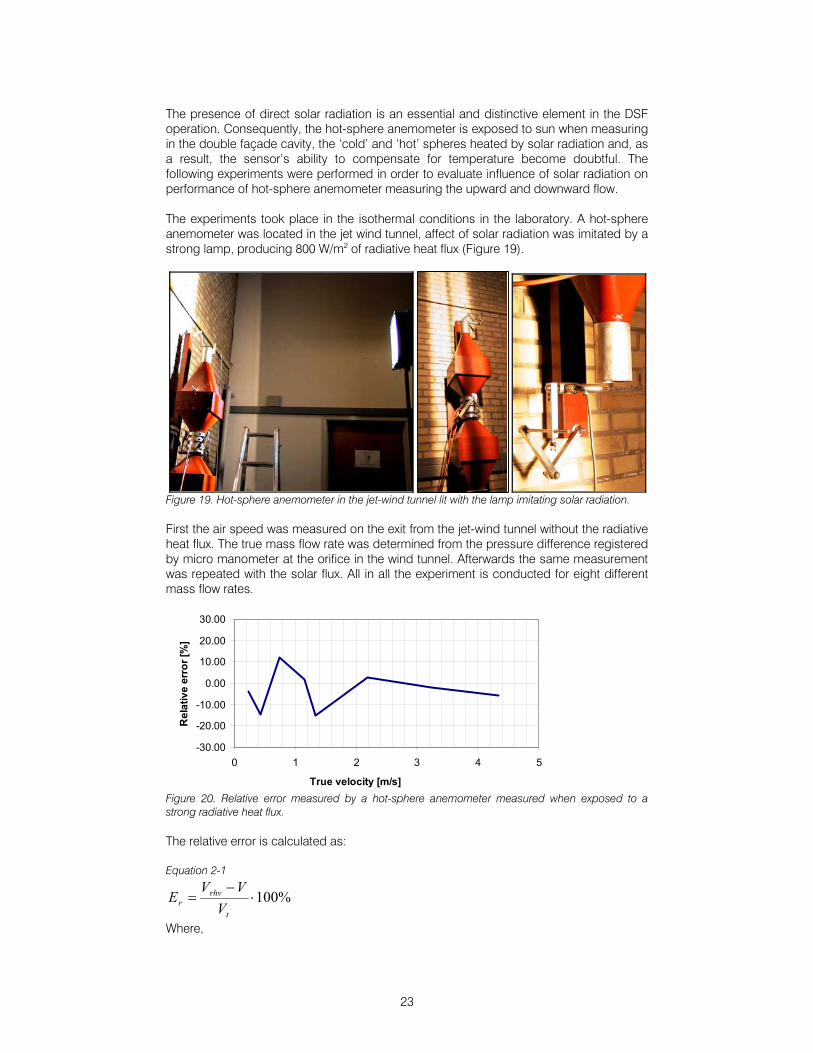
The presence of direct solar radiation is an essential and distinctive element in the DSF operation. Consequently, the hot-sphere anemometer is exposed to sun when measuring in the double façade cavity, the ‘cold’ and ‘hot’ spheres heated by solar radiation and, as a result, the sensor’s ability to compensate for temperature become doubtful. The following experiments were performed in order to evaluate influence of solar radiation on performance of hot-sphere anemometer measuring the upward and downward flow. The experiments took place in the isothermal conditions in the laboratory. A hot-sphere anemometer was located in the jet wind tunnel, affect of solar radiation was imitated by a strong lamp, producing 800 W/m2 of radiative heat flux (Figure 19).
Figure 19. Hot-sphere anemometer in the jet-wind tunnel lit with the lamp imitating solar radiation. First the air speed was measured on the exit from the jet-wind tunnel without the radiative heat flux. The true mass flow rate was determined from the pressure difference registered by micro manometer at the orifice in the wind tunnel. Afterwards the same measurement was repeated with the solar flux. All in all the experiment is conducted for eight different mass flow rates.
-30.00
-20.00
-10.00
0.00
10.00
20.00
30.00
0 1 2 3 4 5
True velocity [m/s]
Rel
ativ
e er
ror [
%]
Figure 20. Relative error measured by a hot-sphere anemometer measured when exposed to a strong radiative heat flux. The relative error is calculated as: Equation 2-1
%100⋅−
=t
rhvr V
VVE
Where,
24
Er - relative error Vrhf - velocity measured with the radiation heat flux V - velocity measured without radiation heat flux Vt - true air velocity in the jet-wind tunnel calculated from orifice If there is any influence of radiation on the performance of the anemometer then it ought to be strongest in the range of low velocities. According to the Figure 20, there is no consistency in the measured relative error. The magnitude of the error varies a lot, and even in the range of the low velocities it is not possible to identify any regularity. One can conclude that the hot-sphere anemometer doesn’t change the performance when exposed to direct solar radiation. This can be explained by two factors. The first one is the surface of the spheres which has very high reflectance property and it is possible that the major part of solar radiation approaching the sphere is reflected. Moreover, the ‘cold’ and ‘hot’ spheres must be heated up equally as both of them are equally exposed, and, as the main principle of the hot-sphere anemometer is the temperature compensation, then equally heated spheres would not affect the temperature compensation. According to the above conclusion the hot-sphere anemometers were used for measurements of the velocity profile in the double façade cavity in the outdoor test facility ‘The Cube’.
2.2.2.3 Testing of the hot-spheres for measurements of the flow direction
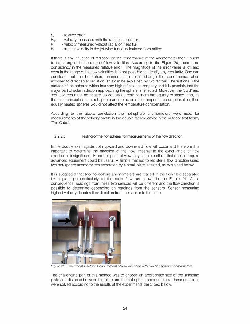
In the double skin façade both upward and downward flow will occur and therefore it is important to determine the direction of the flow, meanwhile the exact angle of flow direction is insignificant. From this point of view, any simple method that doesn’t require advanced equipment could be useful. A simple method to register a flow direction using two hot-sphere anemometers separated by a small plate is tested, as explained below. It is suggested that two hot-sphere anemometers are placed in the flow filed separated by a plate perpendicularly to the main flow, as shown in the Figure 21. As a consequence, readings from these two sensors will be different and the flow direction is possible to determine depending on readings from the sensors. Sensor measuring highest velocity denotes flow direction from the sensor to the plate.
Figure 21. Experimental setup: Measurement of flow direction with two hot-sphere anemometers. The challenging part of this method was to choose an appropriate size of the shielding plate and distance between the plate and the hot-sphere anemometers. These questions were solved according to the results of the experiments described below.
25
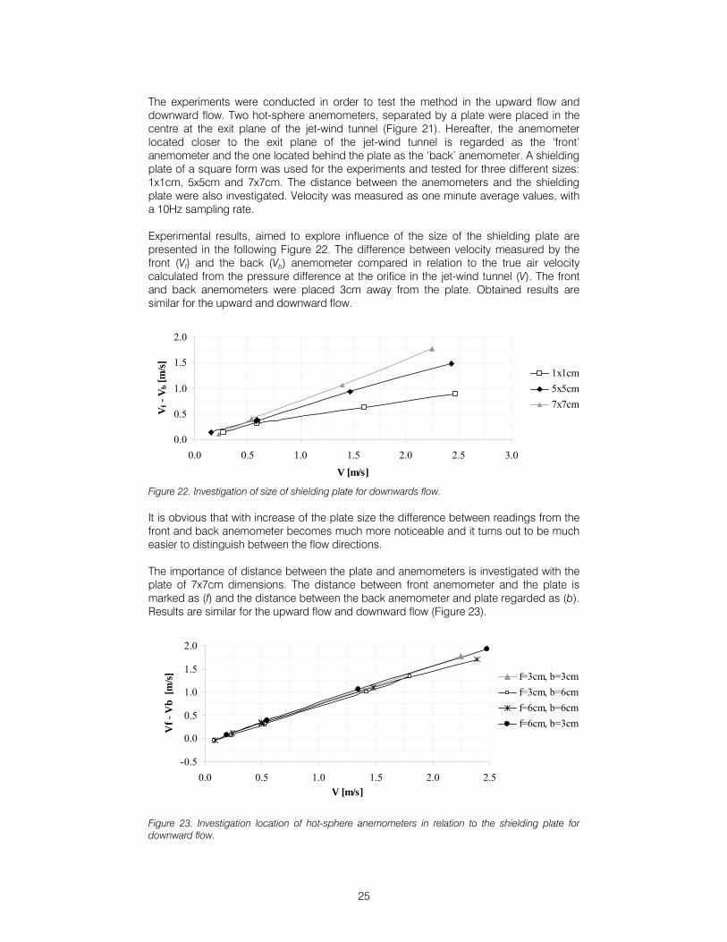
The experiments were conducted in order to test the method in the upward flow and downward flow. Two hot-sphere anemometers, separated by a plate were placed in the centre at the exit plane of the jet-wind tunnel (Figure 21). Hereafter, the anemometer located closer to the exit plane of the jet-wind tunnel is regarded as the ‘front’ anemometer and the one located behind the plate as the ‘back’ anemometer. A shielding plate of a square form was used for the experiments and tested for three different sizes: 1x1cm, 5x5cm and 7x7cm. The distance between the anemometers and the shielding plate were also investigated. Velocity was measured as one minute average values, with a 10Hz sampling rate. Experimental results, aimed to explore influence of the size of the shielding plate are presented in the following Figure 22. The difference between velocity measured by the front (Vf) and the back (Vb) anemometer compared in relation to the true air velocity calculated from the pressure difference at the orifice in the jet-wind tunnel (V). The front and back anemometers were placed 3cm away from the plate. Obtained results are similar for the upward and downward flow.
0.0
0.5
1.0
1.5
2.0
0.0 0.5 1.0 1.5 2.0 2.5 3.0
V [m/s]
Vf -
Vb [
m/s] 1x1cm
5x5cm7x7cm
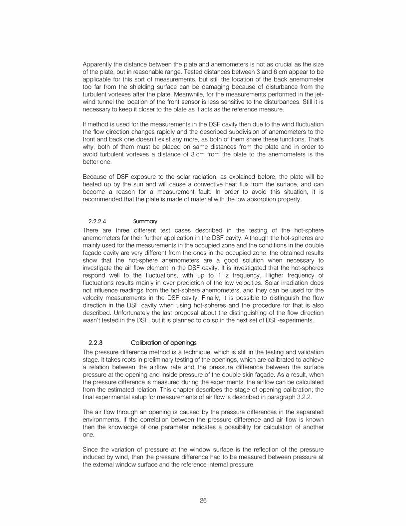
Figure 22. Investigation of size of shielding plate for downwards flow. It is obvious that with increase of the plate size the difference between readings from the front and back anemometer becomes much more noticeable and it turns out to be much easier to distinguish between the flow directions. The importance of distance between the plate and anemometers is investigated with the plate of 7x7cm dimensions. The distance between front anemometer and the plate is marked as (f) and the distance between the back anemometer and plate regarded as (b). Results are similar for the upward flow and downward flow (Figure 23).
-0.5
0.0
0.5
1.0
1.5
2.0
0.0 0.5 1.0 1.5 2.0 2.5V [m/s]
Vf -
Vb
[m/s] f=3cm, b=3cm
f=3cm, b=6cmf=6cm, b=6cmf=6cm, b=3cm
Figure 23. Investigation location of hot-sphere anemometers in relation to the shielding plate for downward flow.
26
Apparently the distance between the plate and anemometers is not as crucial as the size of the plate, but in reasonable range. Tested distances between 3 and 6 cm appear to be applicable for this sort of measurements, but still the location of the back anemometer too far from the shielding surface can be damaging because of disturbance from the turbulent vortexes after the plate. Meanwhile, for the measurements performed in the jet-wind tunnel the location of the front sensor is less sensitive to the disturbances. Still it is necessary to keep it closer to the plate as it acts as the reference measure. If method is used for the measurements in the DSF cavity then due to the wind fluctuation the flow direction changes rapidly and the described subdivision of anemometers to the front and back one doesn’t exist any more, as both of them share these functions. That's why, both of them must be placed on same distances from the plate and in order to avoid turbulent vortexes a distance of 3 cm from the plate to the anemometers is the better one. Because of DSF exposure to the solar radiation, as explained before, the plate will be heated up by the sun and will cause a convective heat flux from the surface, and can become a reason for a measurement fault. In order to avoid this situation, it is recommended that the plate is made of material with the low absorption property.
2.2.2.4 Summary
There are three different test cases described in the testing of the hot-sphere anemometers for their further application in the DSF cavity. Although the hot-spheres are mainly used for the measurements in the occupied zone and the conditions in the double façade cavity are very different from the ones in the occupied zone, the obtained results show that the hot-sphere anemometers are a good solution when necessary to investigate the air flow element in the DSF cavity. It is investigated that the hot-spheres respond well to the fluctuations, with up to 1Hz frequency. Higher frequency of fluctuations results mainly in over prediction of the low velocities. Solar irradiation does not influence readings from the hot-sphere anemometers, and they can be used for the velocity measurements in the DSF cavity. Finally, it is possible to distinguish the flow direction in the DSF cavity when using hot-spheres and the procedure for that is also described. Unfortunately the last proposal about the distinguishing of the flow direction wasn’t tested in the DSF, but it is planned to do so in the next set of DSF-experiments.
2.2.3 Calibration of openings The pressure difference method is a technique, which is still in the testing and validation stage. It takes roots in preliminary testing of the openings, which are calibrated to achieve a relation between the airflow rate and the pressure difference between the surface pressure at the opening and inside pressure of the double skin façade. As a result, when the pressure difference is measured during the experiments, the airflow can be calculated from the estimated relation. This chapter describes the stage of opening calibration; the final experimental setup for measurements of air flow is described in paragraph 3.2.2. The air flow through an opening is caused by the pressure differences in the separated environments. If the correlation between the pressure difference and air flow is known then the knowledge of one parameter indicates a possibility for calculation of another one. Since the variation of pressure at the window surface is the reflection of the pressure induced by wind, then the pressure difference had to be measured between pressure at the external window surface and the reference internal pressure.
27
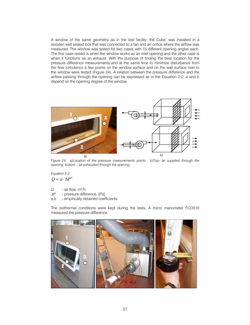
A window of the same geometry as in the test facility ‘the Cube’ was installed in a wooden well sealed box that was connected to a fan and an orifice where the airflow was measured. The window was tested for two cases with 15 different opening angles each. The first case tested is when the window works as an inlet opening and the other case is when it functions as an exhaust. With the purpose of finding the best location for the pressure difference measurements and at the same time to minimize disturbance from the flow turbulence a few points on the window surface and on the wall surface next to the window were tested (Figure 24). A relation between the pressure difference and the airflow passing through the opening can be expressed as in the Equation 2-2, a and b depend on the opening degree of the window.
a) Figure 24. a)Location of the pressure measurements points. b)Top- air supplied through the opening, bottom – air exhausted through the opening. Equation 2-2
bPaQ Δ⋅= Q - air flow, m3/h ΔP - pressure difference, [Pa] a,b - empirically obtained coefficients The isothermal conditions were kept during the tests. A micro manometer FCO510 measured the pressure difference.
b)
1
2
3
1
2
3
28
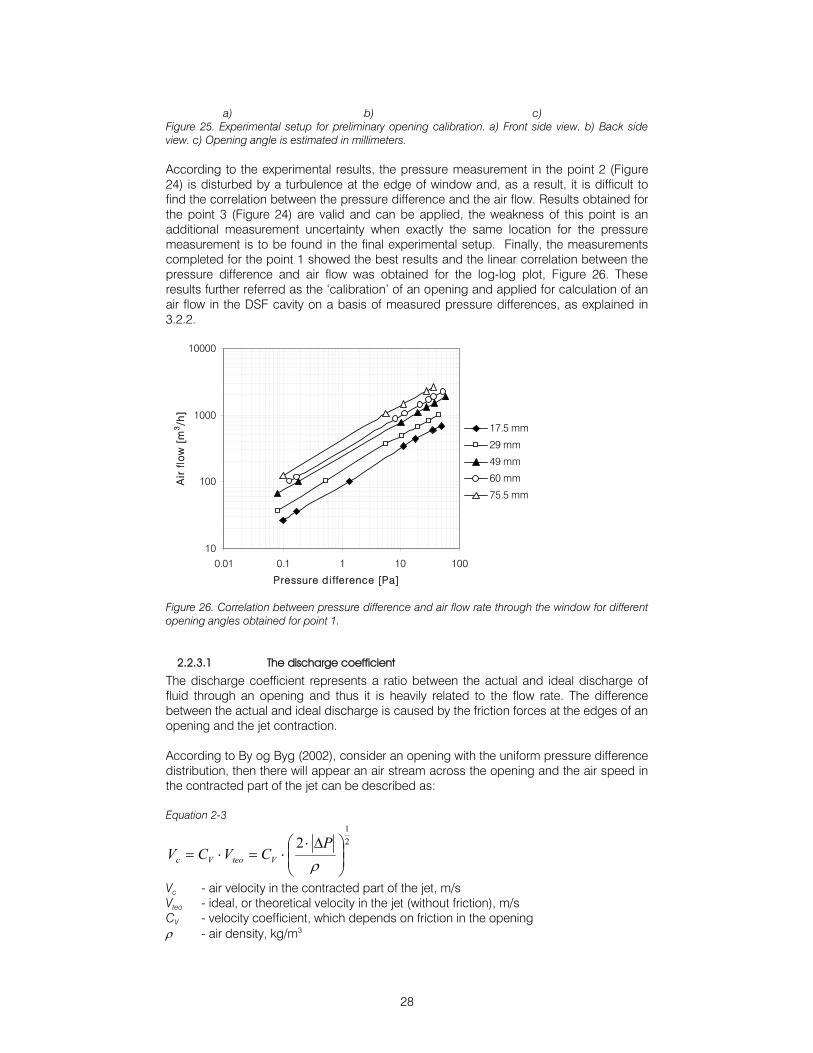
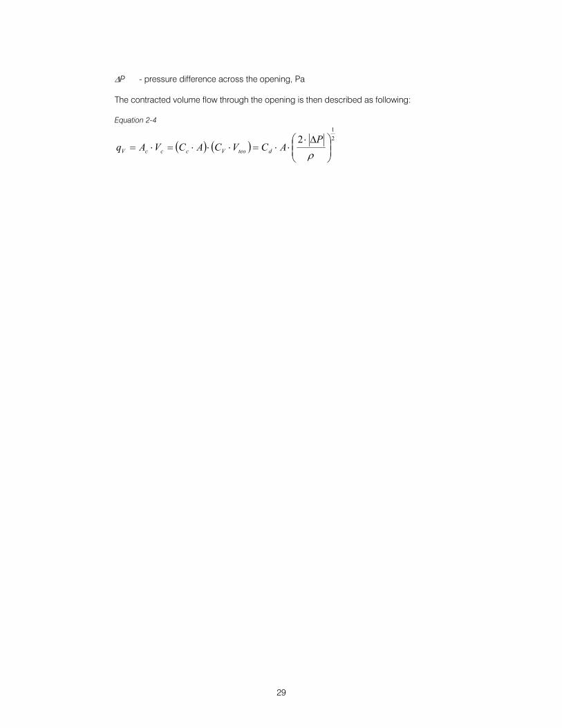
a) b) c) Figure 25. Experimental setup for preliminary opening calibration. a) Front side view. b) Back side view. c) Opening angle is estimated in millimeters. According to the experimental results, the pressure measurement in the point 2 (Figure 24) is disturbed by a turbulence at the edge of window and, as a result, it is difficult to find the correlation between the pressure difference and the air flow. Results obtained for the point 3 (Figure 24) are valid and can be applied, the weakness of this point is an additional measurement uncertainty when exactly the same location for the pressure measurement is to be found in the final experimental setup. Finally, the measurements completed for the point 1 showed the best results and the linear correlation between the pressure difference and air flow was obtained for the log-log plot, Figure 26. These results further referred as the ‘calibration’ of an opening and applied for calculation of an air flow in the DSF cavity on a basis of measured pressure differences, as explained in 3.2.2.
10
100
1000
10000
0.01 0.1 1 10 100
Pressure d i fference [Pa]
Air
flo
w [
m3/h
]
17.5 mm
29 mm
49 mm
60 mm
75.5 mm
Figure 26. Correlation between pressure difference and air flow rate through the window for different opening angles obtained for point 1.
2.2.3.1 The discharge coefficient
The discharge coefficient represents a ratio between the actual and ideal discharge of fluid through an opening and thus it is heavily related to the flow rate. The difference between the actual and ideal discharge is caused by the friction forces at the edges of an opening and the jet contraction. According to By og Byg (2002), consider an opening with the uniform pressure difference distribution, then there will appear an air stream across the opening and the air speed in the contracted part of the jet can be described as: Equation 2-3
21
2⎟⎟⎠
⎞⎜⎜⎝
⎛ Δ⋅⋅=⋅=
ρP
CVCV VteoVc
Vc - air velocity in the contracted part of the jet, m/s Vteo - ideal, or theoretical velocity in the jet (without friction), m/s CV - velocity coefficient, which depends on friction in the opening ρ - air density, kg/m3
29
ΔP - pressure difference across the opening, Pa The contracted volume flow through the opening is then described as following: Equation 2-4
( ) ( )21
2⎟⎟⎠
⎞⎜⎜⎝
⎛ Δ⋅⋅⋅=⋅⋅⋅=⋅=
ρP
ACVCACVAq dteoVcccV
30
Then: Equation 2-5
cVd CCC ⋅=
Where, qv - volume flow, m3/s Ac - contracted area of the jet, m2
A - geometry correct area of the opening, m2
Cc - contraction coefficient of the jet for the particular opening Cd - discharge coefficient of the particular opening Considering the experimental data available from the above section 2.2.3, one is able to calculate the discharge coefficient for every opening degree, as following: Equation 2-6
ρP
A
qC V
dΔ⋅
⋅
=2
The discharge coefficients in the experimental set-up were calculated, according to the above expression and the results of calculations were further used in the empirical test case specification, see Kalyanova & Heiselberg (2007).
31
33.. THE FULL-SCALE MEASUREMENTS
The content of this section is addressed to the full-scale experiments conducted in the experimental test facility ‘the Cube’, in a period September-December, 2006. Experimental results contain of three modes of the DSF performance:
• MODE 1: External air curtain mode (01.10.2006 – 15.10.2006) • MODE 2: Transparent insulation mode (19.10.2006 - 06.11.2006) • MODE 3: Preheating mode (09-11-2006 - 30-11-2006)
Certainly, the application of the results set the main constrains in a design of the experimental setup. Besides the measurements in the DSF, both the weather conditions and the conditions in the experiment room as a reflection of the DSF performance were registered.
3.1 MODES OF THE DSF PERFORMANCE IN THE EXPERIMENTS
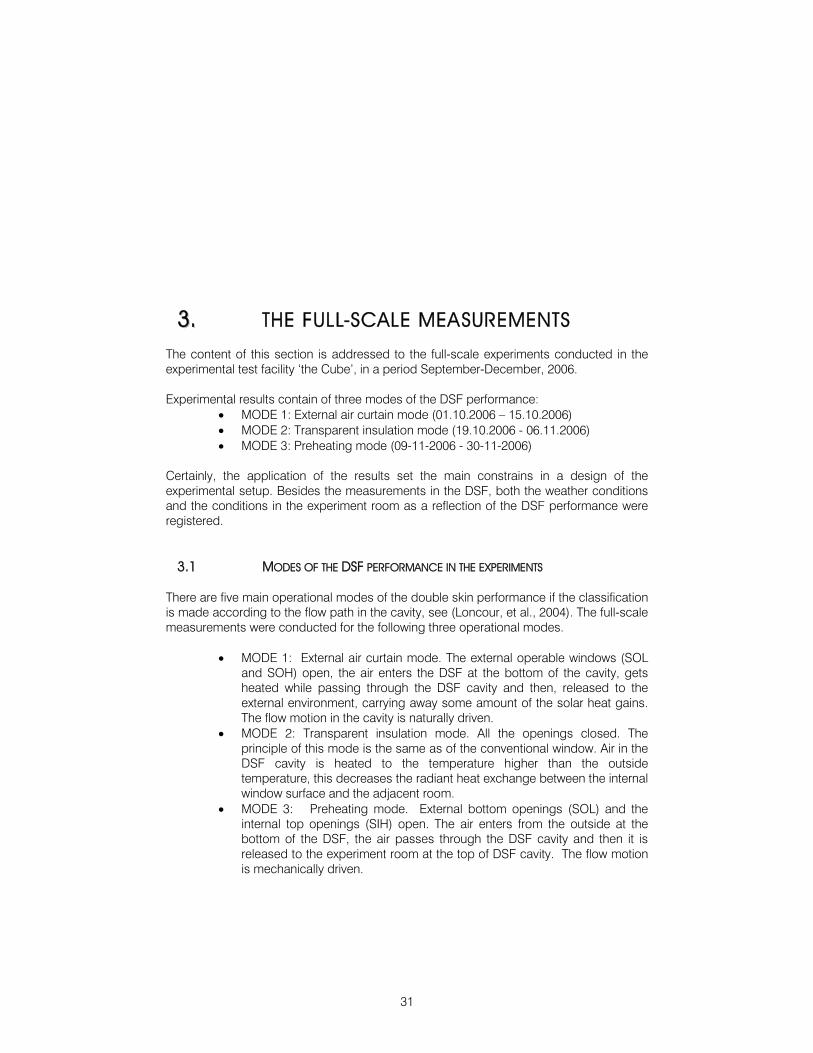
There are five main operational modes of the double skin performance if the classification is made according to the flow path in the cavity, see (Loncour, et al., 2004). The full-scale measurements were conducted for the following three operational modes.
• MODE 1: External air curtain mode. The external operable windows (SOL and SOH) open, the air enters the DSF at the bottom of the cavity, gets heated while passing through the DSF cavity and then, released to the external environment, carrying away some amount of the solar heat gains. The flow motion in the cavity is naturally driven.
• MODE 2: Transparent insulation mode. All the openings closed. The principle of this mode is the same as of the conventional window. Air in the DSF cavity is heated to the temperature higher than the outside temperature, this decreases the radiant heat exchange between the internal window surface and the adjacent room.
• MODE 3: Preheating mode. External bottom openings (SOL) and the internal top openings (SIH) open. The air enters from the outside at the bottom of the DSF, the air passes through the DSF cavity and then it is released to the experiment room at the top of DSF cavity. The flow motion is mechanically driven.
32
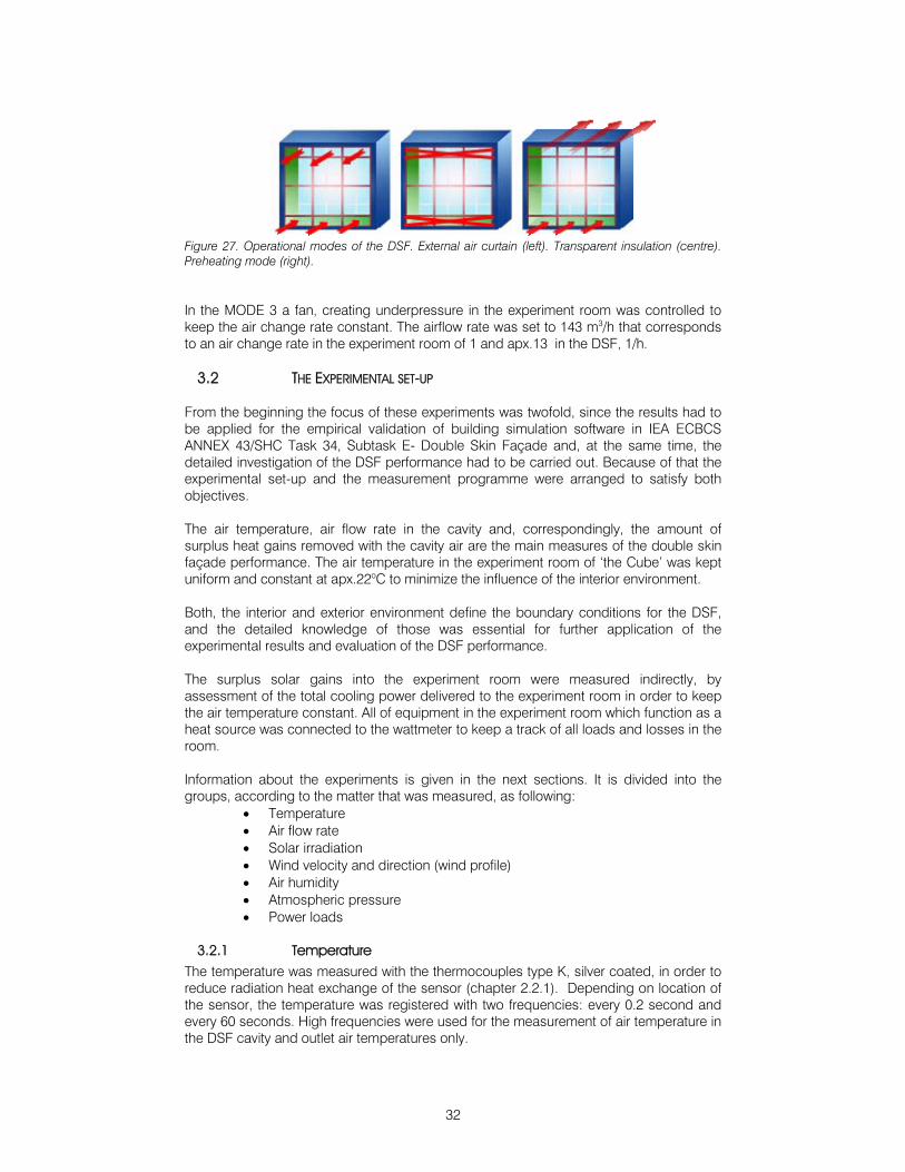
Figure 27. Operational modes of the DSF. External air curtain (left). Transparent insulation (centre). Preheating mode (right).
In the MODE 3 a fan, creating underpressure in the experiment room was controlled to keep the air change rate constant. The airflow rate was set to 143 m3/h that corresponds to an air change rate in the experiment room of 1 and apx.13 in the DSF, 1/h.
3.2 THE EXPERIMENTAL SET-UP
From the beginning the focus of these experiments was twofold, since the results had to be applied for the empirical validation of building simulation software in IEA ECBCS ANNEX 43/SHC Task 34, Subtask E- Double Skin Façade and, at the same time, the detailed investigation of the DSF performance had to be carried out. Because of that the experimental set-up and the measurement programme were arranged to satisfy both objectives. The air temperature, air flow rate in the cavity and, correspondingly, the amount of surplus heat gains removed with the cavity air are the main measures of the double skin façade performance. The air temperature in the experiment room of ‘the Cube’ was kept uniform and constant at apx.22oC to minimize the influence of the interior environment. Both, the interior and exterior environment define the boundary conditions for the DSF, and the detailed knowledge of those was essential for further application of the experimental results and evaluation of the DSF performance. The surplus solar gains into the experiment room were measured indirectly, by assessment of the total cooling power delivered to the experiment room in order to keep the air temperature constant. All of equipment in the experiment room which function as a heat source was connected to the wattmeter to keep a track of all loads and losses in the room. Information about the experiments is given in the next sections. It is divided into the groups, according to the matter that was measured, as following:
• Temperature • Air flow rate • Solar irradiation • Wind velocity and direction (wind profile) • Air humidity • Atmospheric pressure • Power loads
3.2.1 Temperature
The temperature was measured with the thermocouples type K, silver coated, in order to reduce radiation heat exchange of the sensor (chapter 2.2.1). Depending on location of the sensor, the temperature was registered with two frequencies: every 0.2 second and every 60 seconds. High frequencies were used for the measurement of air temperature in the DSF cavity and outlet air temperatures only.
33
The air temperature was measured in the engine room (tc 11, where tc xx – is a sign for a thermocouple with the number xx), instrument room (tc 4), DSF, experiment room. The outside air temperature was measured in 2 points (tc 67, tc 77), at the height 2 m above the ground (thermocouples). The ground temperature, underneath of foundation in the experiment room (tc 51, tc 52).
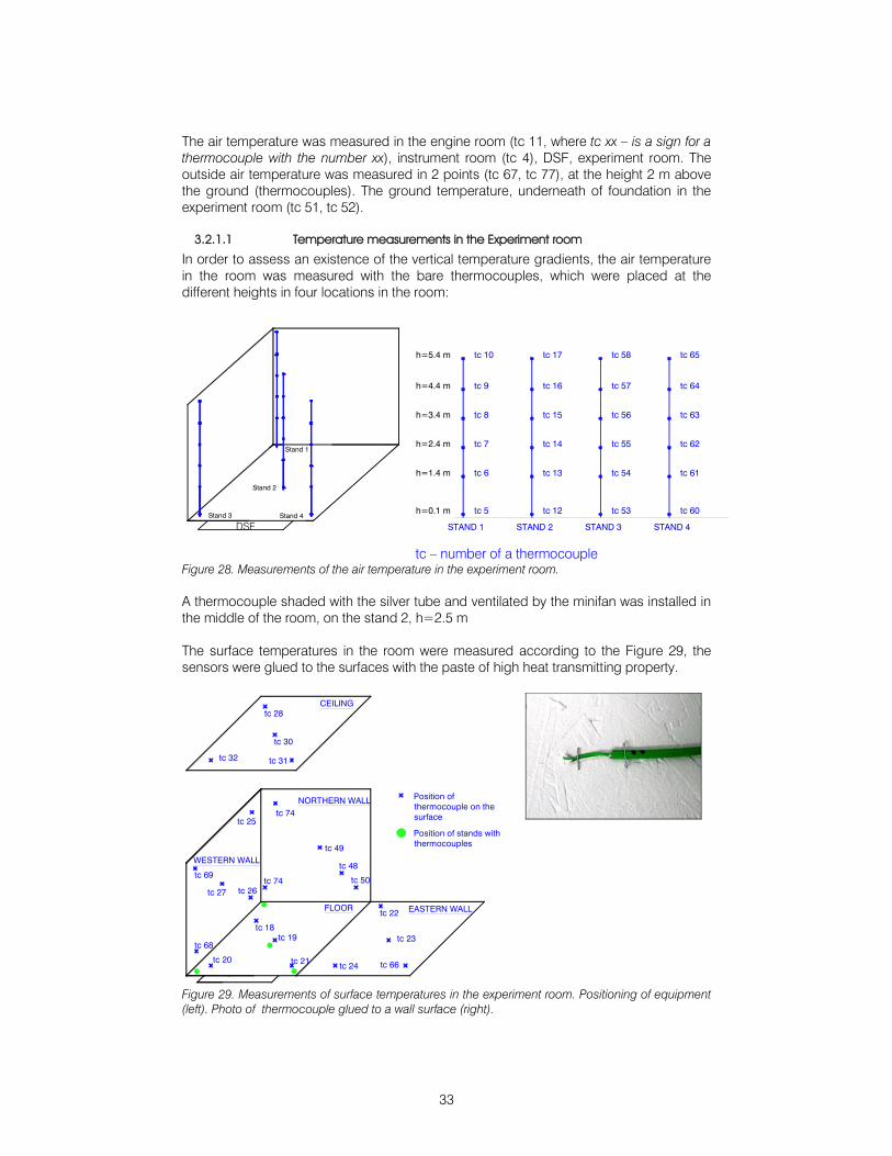
3.2.1.1 Temperature measurements in the Experiment room
In order to assess an existence of the vertical temperature gradients, the air temperature in the room was measured with the bare thermocouples, which were placed at the different heights in four locations in the room:
STAND 1
tc 5
tc 6
tc 7
tc 8
tc 9
tc 10
h=0.1 m
h=1.4 m
h=5.4 m
h=4.4 m
h=3.4 m
h=2.4 m
tc 17
tc 16
tc 15
tc 14
tc 13
tc 12
STAND 2 STAND 3
tc 53
tc 54
tc 55
tc 56
tc 57
tc 58 tc 65
tc 64
tc 63
tc 62
tc 61
tc 60
STAND 4
tc – number of a thermocouple Figure 28. Measurements of the air temperature in the experiment room. A thermocouple shaded with the silver tube and ventilated by the minifan was installed in the middle of the room, on the stand 2, h=2.5 m The surface temperatures in the room were measured according to the Figure 29, the sensors were glued to the surfaces with the paste of high heat transmitting property.
tc 31
tc 30
tc 28
tc 32
CEILING
WESTERN WALL
tc 66
tc 22
tc 23
tc 24tc 21
tc 19
tc 20
tc 18
tc 26tc 27
tc 25
tc 68
tc 69
FLOOR
NORTHERN WALL
tc 74 tc 50
tc 48
tc 49
tc 74
EASTERN WALL
Position of stands with thermocouples
Position of thermocouple on the surface
Figure 29. Measurements of surface temperatures in the experiment room. Positioning of equipment (left). Photo of thermocouple glued to a wall surface (right).
DSF Stand 4 Stand 3
Stand 2
Stand 1
34
3.2.1.2 Temperature measurements in the DSF
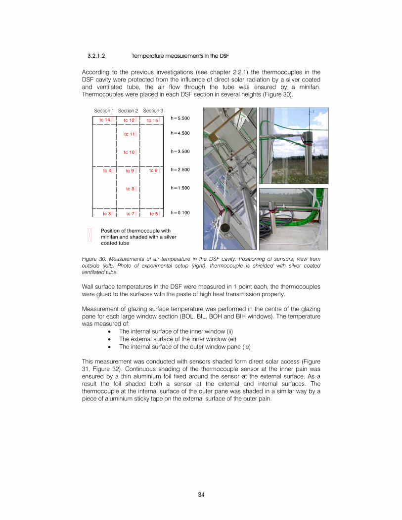
According to the previous investigations (see chapter 2.2.1) the thermocouples in the DSF cavity were protected from the influence of direct solar radiation by a silver coated and ventilated tube, the air flow through the tube was ensured by a minifan. Thermocouples were placed in each DSF section in several heights (Figure 30).
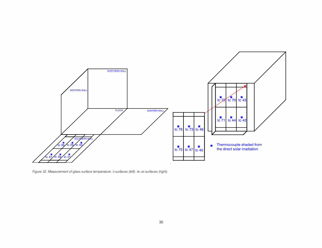
Figure 30. Measurements of air temperature in the DSF cavity. Positioning of sensors, view from outside (left). Photo of experimental setup (right), thermocouple is shielded with silver coated ventilated tube. Wall surface temperatures in the DSF were measured in 1 point each, the thermocouples were glued to the surfaces with the paste of high heat transmission property. Measurement of glazing surface temperature was performed in the centre of the glazing pane for each large window section (BOL, BIL, BOH and BIH windows). The temperature was measured of:
• The internal surface of the inner window (ii) • The external surface of the inner window (ei) • The internal surface of the outer window pane (ie)
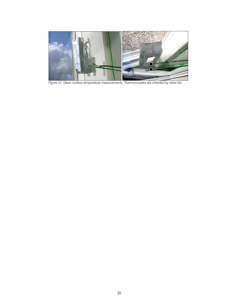
This measurement was conducted with sensors shaded form direct solar access (Figure 31, Figure 32). Continuous shading of the thermocouple sensor at the inner pain was ensured by a thin aluminium foil fixed around the sensor at the external surface. As a result the foil shaded both a sensor at the external and internal surfaces. The thermocouple at the internal surface of the outer pane was shaded in a similar way by a piece of aluminium sticky tape on the external surface of the outer pain.
Section 1 Section 2 Section 3
h=0.100
h=1.500
h=2.500
h=3.500
h=4.500
h=5.500
tc 5tc 7tc 3
tc 8
tc 4 tc 9 tc 6
tc 10
tc 11
tc 12tc 14 tc 15
Position of thermocouple with minifan and shaded with a silver coated tube
35
Figure 31. Glass surface temperature measurements. Thermocouples are shielded by silver foil.
36
SOUTHERN WALL
WESTERN WALL
tc 29
tc 39
tc 40
tc 41tc 37
tc 36
FLOOR
NORTHERN WALL
EASTERN WALL
.
tc 72 tc 70 tc 43
tc 42tc 44tc 71
tc 76 tc 73 tc 46
tc 75 tc 47 tc 45
Thermocouple shaded from the direct solar irradiation
Figure 32. Measurement of glass surface temperature. ii-surfaces (left). ie-,ei-surfaces (right).
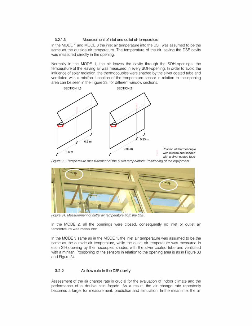
3.2.1.3 Measurement of inlet and outlet air temperature
In the MODE 1 and MODE 3 the inlet air temperature into the DSF was assumed to be the same as the outside air temperature. The temperature of the air leaving the DSF cavity was measured directly in the opening. Normally in the MODE 1, the air leaves the cavity through the SOH-openings, the temperature of the leaving air was measured in every SOH-opening. In order to avoid the influence of solar radiation, the thermocouples were shaded by the silver coated tube and ventilated with a minifan. Location of the temperature sensor in relation to the opening area can be seen in the Figure 33, for different window sections.
Position of thermocouple with minifan and shaded with a silver coated tube
0.6 m
0.6 m0.25 m
0.95 m
SECTION 1,3 SECTION 2
Figure 33. Temperature measurement of the outlet temperature. Positioning of the equipment
Figure 34. Measurement of outlet air temperature from the DSF. In the MODE 2, all the openings were closed, consequently no inlet or outlet air temperature was measured. In the MODE 3 same as in the MODE 1, the inlet air temperature was assumed to be the same as the outside air temperature, while the outlet air temperature was measured in each SIH-opening by thermocouples shaded with the silver coated tube and ventilated with a minifan. Positioning of the sensors in relation to the opening area is as in Figure 33 and Figure 34.
3.2.2 Air flow rate in the DSF cavity
Assessment of the air change rate is crucial for the evaluation of indoor climate and the performance of a double skin façade. As a result, the air change rate repeatedly becomes a target for measurement, prediction and simulation. In the meantime, the air
38
flow occurred in the naturally ventilated spaces is very intricate and extremely difficult to measure. The stochastic nature of wind and as a consequence non-uniform and dynamic flow conditions in combination with the assisting or opposing buoyancy force cause the main difficulties. In the literature, there are three methods used for estimation of the air change rate in a naturally ventilated space. These are the tracer gas method, method of calculating the air flow from the measured velocity profiles in an opening or calculated from the expressions for the natural ventilation or scale modelling, see (Larsen, 2006 and Hitchin & Wilson, 1967), which involves measurements of air temperature, wind speed, wind direction, wind pressure coefficients on the surfaces and pressure drop across the opening. Experimental investigation of the airflow rate requires measurement of many highly fluctuating parameters. The fluctuation frequency implies the high sampling frequency for the measurements. For example according to Larsen (2006), the wind speed has to be measured at least at the frequency of 5 Hz, otherwise peaks in the wind velocity can be lost when averaged in time. As a consequence, measurements of the airflow rate are limited to time and costs. When measured with the tracer gas method the limitations are extended to the airflow rates, as with the high airflow rate the amount of injected tracer gas will be enormous. Because of these, the investigation of the natural air flow often is carried out in the controlled environment of the wind tunnel or scale models. This section addresses the experimental setup for measurements of the air flow rate in the DSF cavity of ‘the Cube’. There are three techniques used for the air flow measurements, these are:
• Velocity profile method • Tracer gas method • Pressure difference method
Velocity profile method This method requires a set of anemometers to measure a velocity profile in the opening, and then the shape of the determined velocity profile depends on amount of anemometers installed. At the same time, the equipment located directly in the opening can become an obstruction for the flow appearance. Thus, the method becomes a trade off between the maximum desired amount of anemometers and the minimum desired flow obstruction. Instead of placing equipment directly in the opening in the case of the double skin façade, it can be placed in the DSF cavity, where the velocity profile can be measured in a few levels instead for one. For the double skin façade, the negative aspect of this method is explained by airflow variation, as the instantaneous air velocity in the cavity may vary from 0 to 5 m/s. This velocity range is challenging, as the equipment must be suitable for measurements of both low and higher velocities, moreover, it is necessary to be able to detect the reverse flow appearance and follow the flow fluctuations. As explained earlier in 2.2.2.2, the hot-sphere anemometers have proved to be suitable for the task. Temperature compensation is the main working principle of the hot sphere anemometers, therefore measurements of air velocity under the direct solar radiation access can be an issue for the accuracy of the experiments. In order to prevent this kind of error the hot sphere anemometers were preliminary tested and calibrated under the artificial sun conditions, in the wind tunnel, see chapter 2.2.2.
39
Accuracy of the velocity profile method depends on many factors. Therefore it is common to express it in accuracy of the measuring equipment. The hot sphere anemometers have been calibrated and had an accuracy of 0.01m/s. Tracer gas method This method requires the minimum amount of measurements and equipment, but it is characterized with frequent difficulties to obtain uniform concentration of the tracer gas, disturbances from the wind wash-out effects and finally with the time delay of signal caused by the time constant of gas analyzer. The constant injection method (Etheridge, 1996) is used in the experiments described in following sections. Talking about the accuracy of these measurements, one can speak only of accuracy of equipment used for the measurement, as it is not possible to give estimation for the dataset accuracy for the whole measurement period. This is partly caused by the dynamics of the measured air flow, where the measurement accuracy will change along with the changes of boundary conditions. Another reason is simply the lack of information and experience for this kind of measurement in outdoor test facilities. Still, one can refer to the literature about the accuracy of the experimental method used. According to McWilliams (2002), the tracer gas theory assumes that the tracer gas concentration is constant throughout the measured zone. The expected error of tracer gas results is in the range of 5-10%, what greatly depends on the tracer gas mixing with the air in the DSF cavity. Pressure difference method The pressure difference method is a technique, which is still in the testing and validation stage. It takes roots in preliminary testing of the openings, which calibrated to achieve a relation between the airflow rate and the pressure difference between the surface pressure at the opening and inside pressure of the double skin façade. As a result, when the pressure difference is measured during the experiments, the airflow can be calculated from the estimated relation. The procedure for calibration of openings is described in chapter 2.2.3.
3.2.2.1 Experimental setup
The velocity profile method During the experiments in ‘the Cube’ all of the velocity measurements were conducted in the section 2 (Figure 7), the velocity profiles were measured in 3-6 levels, with the various number of anemometers in different levels. Different amount of levels was used for different DSF operational modes. Levels are numbered with the Roman numbers in the Figure 35. All in all 46 of hot-sphere anemometers were installed in the experimental setup (Figure 36), 34 of them were engaged in the measurements of the velocity profiles in different levels of the DSF cavity. The measurement frequency of the hot-sphere anemometers is 10Hz.
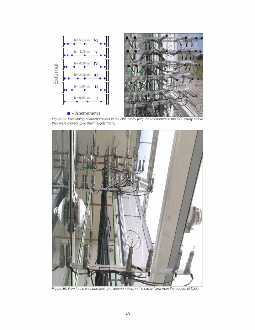
40
V
IV
III
II
I
h= 5.15 m
h= 4.70 m
h= 4.36 m
h= 2.50 m
h= 1.91 m
h= 0.95 m
Ext
erna
l
- Anemometer
VI
Figure 35. Positioning of anemometers in the DSF cavity (left). Anemometers in the DSF cavity before they were moved up to their heights (right).
Figure 36. View to the final positioning of anemometers in the cavity (view from the bottom of DSF).
41
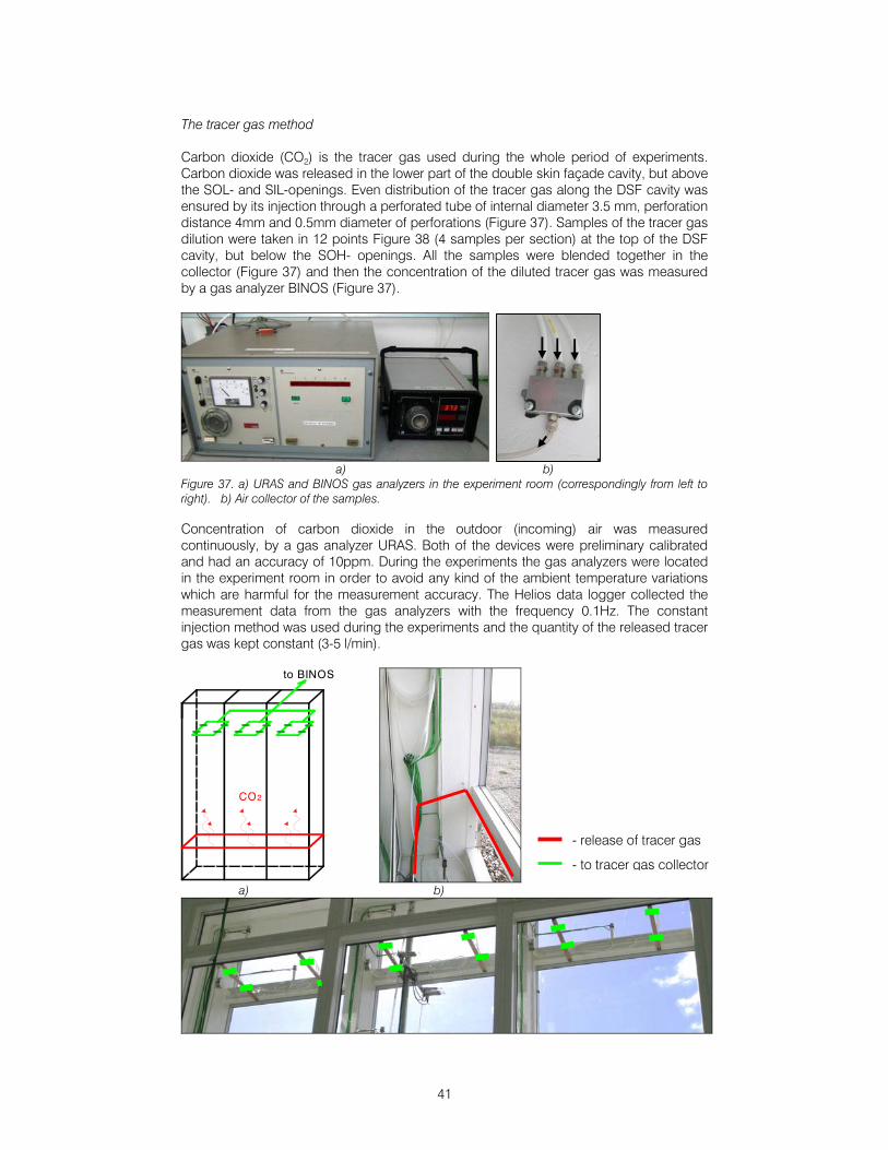
The tracer gas method Carbon dioxide (CO2) is the tracer gas used during the whole period of experiments. Carbon dioxide was released in the lower part of the double skin façade cavity, but above the SOL- and SIL-openings. Even distribution of the tracer gas along the DSF cavity was ensured by its injection through a perforated tube of internal diameter 3.5 mm, perforation distance 4mm and 0.5mm diameter of perforations (Figure 37). Samples of the tracer gas dilution were taken in 12 points Figure 38 (4 samples per section) at the top of the DSF cavity, but below the SOH- openings. All the samples were blended together in the collector (Figure 37) and then the concentration of the diluted tracer gas was measured by a gas analyzer BINOS (Figure 37).
a) b) Figure 37. a) URAS and BINOS gas analyzers in the experiment room (correspondingly from left to right). b) Air collector of the samples. Concentration of carbon dioxide in the outdoor (incoming) air was measured continuously, by a gas analyzer URAS. Both of the devices were preliminary calibrated and had an accuracy of 10ppm. During the experiments the gas analyzers were located in the experiment room in order to avoid any kind of the ambient temperature variations which are harmful for the measurement accuracy. The Helios data logger collected the measurement data from the gas analyzers with the frequency 0.1Hz. The constant injection method was used during the experiments and the quantity of the released tracer gas was kept constant (3-5 l/min).
to BINOS
CO2
a) b)
- release of tracer gas
- to tracer gas collector
42
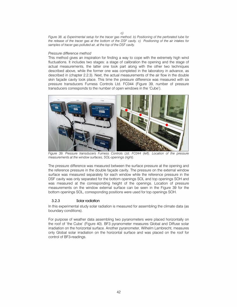
c) Figure 38. a) Experimental setup for the tracer gas method. b) Positioning of the perforated tube for the release of the tracer gas at the bottom of the DSF cavity. c) Positioning of the air intakes for samples of tracer gas polluted air, at the top of the DSF cavity. Pressure difference method This method gives an inspiration for finding a way to cope with the extremely high wind fluctuations. It includes two stages: a stage of calibration the opening and the stage of actual measurements, the latter one took part along with the other two techniques described above, while the former one was completed in the laboratory in advance, as described in (chapter 2.2.3). Next, the actual measurements of the air flow in the double skin façade cavity took place. This time the pressure difference was measured with six pressure transducers Furness Controls Ltd. FC044 (Figure 39, number of pressure transducers corresponds to the number of open windows in the ‘Cube’).
Figure 39. Pressure transducers Furness Controls Ltd. FC044 (left). Location of the pressure measurements at the window surfaces, SOL-openings (right). The pressure difference was measured between the surface pressure at the opening and the reference pressure in the double façade cavity. The pressure on the external window surface was measured separately for each window while the reference pressure in the DSF cavity was only separated for the bottom openings SOL and top openings SOH and was measured at the corresponding height of the openings. Location of pressure measurements on the window external surface can be seen in the Figure 39 for the bottom openings SOL, corresponding positions were used for top openings SOH.
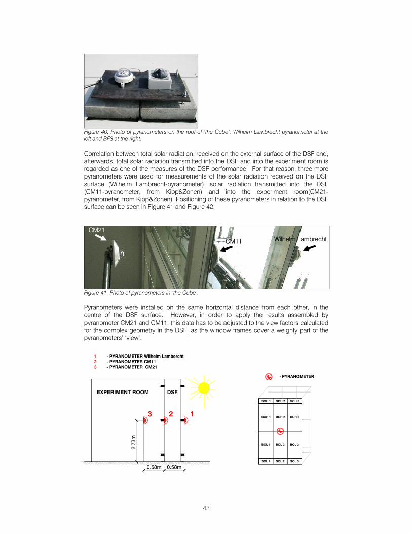
3.2.3 Solar radiation In this experimental study solar radiation is measured for assembling the climate data (as boundary conditions). For purpose of weather data assembling two pyranometers were placed horizontally on the roof of ‘the Cube’ (Figure 40). BF3 pyranometer measures Global and Diffuse solar irradiation on the horizontal surface. Another pyranometer, Wilhelm Lambrecht, measures only Global solar irradiation on the horizontal surface and was placed on the roof for control of BF3-readings.
43
Figure 40. Photo of pyranometers on the roof of ‘the Cube’, Wilhelm Lambrecht pyranometer at the left and BF3 at the right. Correlation between total solar radiation, received on the external surface of the DSF and, afterwards, total solar radiation transmitted into the DSF and into the experiment room is regarded as one of the measures of the DSF performance. For that reason, three more pyranometers were used for measurements of the solar radiation received on the DSF surface (Wilhelm Lambrecht-pyranometer), solar radiation transmitted into the DSF (CM11-pyranometer, from Kipp&Zonen) and into the experiment room(CM21-pyranometer, from Kipp&Zonen). Positioning of these pyranometers in relation to the DSF surface can be seen in Figure 41 and Figure 42.
Figure 41. Photo of pyranometers in ‘the Cube’. Pyranometers were installed on the same horizontal distance from each other, in the centre of the DSF surface. However, in order to apply the results assembled by pyranometer CM21 and CM11, this data has to be adjusted to the view factors calculated for the complex geometry in the DSF, as the window frames cover a weighty part of the pyranometers’ ‘view’.
1 - PYRANOMETER Wilhelm Lambercht2 - PYRANOMETER CM113 - PYRANOMETER CM21
DSF
2.73
m
0.58m
0.58m
EXPERIMENT ROOM
123
SOL 1 SOL 2 SOL 3
SOH 1 SOH 2 SOH 3
BOH 1 BOH 2 BOH 3
BOL 1 BOL 2 BOL 3
- PYRANOMETER
CM11
CM21 Wilhelm Lambrecht
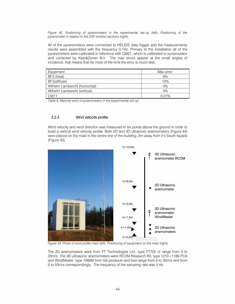
44
Figure 42. Positioning of pyranometers in the experimental set-up (left). Positioning of the pyranometer in relation to the DSF window sections (right). All of the pyranometers were connected to HELIOS data logger and the measurements results were assembled with the frequency 0.1Hz. Primary to the installation all of the pyranometers were calibrated in reference with CM21, which is calibrated in sunsimulator and corrected by Kipp&Zonen B.V. The max errors appear at the small angles of incidence, that means that for most of the time the error is much less. Equipment Max error: BF3 (total) 6% BF3(diffuse) 10% Wilhelm Lambercht (horizontal) 3% Wilhelm Lambercht (vertical) 5% CM11 0.01% Table 8. Maximal error of pyranometers in the experimental set-up.
3.2.4 Wind velocity profile Wind velocity and wind direction was measured in six points above the ground in order to build a vertical wind velocity profile. Both 2D and 3D ultrasonic anemometers (Figure 44) were placed on the mast in the centre line of the building, 2m away from it’s South façade (Figure 43).
h=10.0m
h=6.0m
h=3.0m
h=1.5m
h=0.5m
h=1.0m
3D Ultrasonic anemometer RCOM
2D Ultrasonic anemometer
3D Ultrasonic anemometer WindMaster
2D Ultrasonic anemometers
Figure 43. Photo of wind profile mast (left). Positioning of equipment on the mast (right). The 2D anemometers were from FT Technologies Ltd., type FT702 of range from 0 to 30m/s. The 3D ultrasonic anemometers were RCOM Research R3, type 1210+1189 PCA and WindMaster, type 1086M from Gill producer and had range from 0 to 30m/s and from 0 to 50m/s correspondingly. The frequency of the sampling rate was 5 Hz.
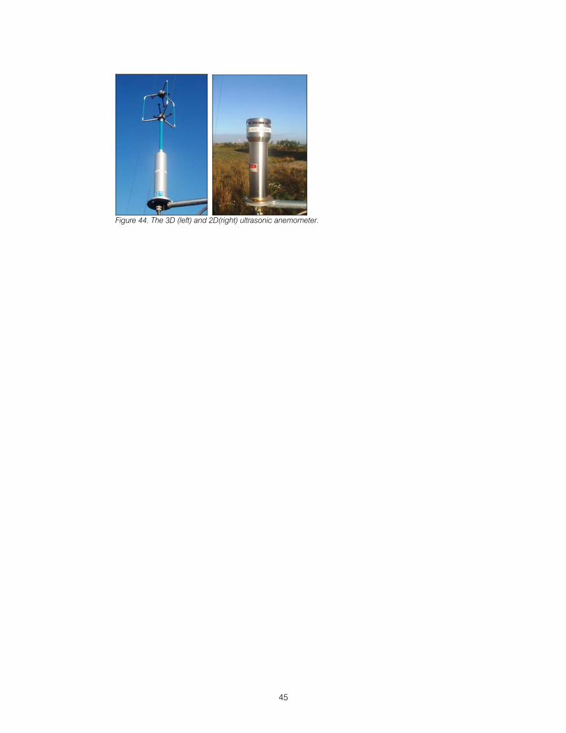
45
Figure 44. The 3D (left) and 2D(right) ultrasonic anemometer.
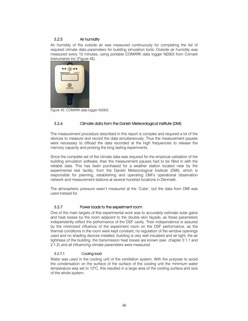
46
3.2.5 Air humidity Air humidity of the outside air was measured continuously for completing the list of required climate data parameters for building simulation tools. Outside air humidity was measured every 10 minutes, using portable COMARK data logger N2003 from Comark Instruments Inc (Figure 45).
Figure 45. COMARK data logger N2003.
3.2.6 Climate data from the Danish Meteorological Institute (DMI) The measurement procedure described in this report is complex and required a lot of the devices to measure and record the data simultaneously. Thus the measurement pauses were necessary to offload the data recorded at the high frequencies to release the memory capacity and prolong the long lasting experiments. Since the complete set of the climate data was required for the empirical validation of the building simulation software, than the measurement pauses had to be filled in with the reliable data. This has been purchased for a weather station located near by the experimental test facility, from the Danish Meteorological Institute (DMI), which is responsible for planning, establishing and operating DMI’s operational observation network and measurement stations at several hundred locations in Denmark. The atmospheric pressure wasn’t measured at the ‘Cube’, but the data from DMI was used instead for.
3.2.7 Power loads to the experiment room One of the main targets of this experimental work was to accurately estimate solar gains and heat losses by the room adjacent to the double skin façade, as these parameters independently reflect the performance of the DSF cavity. Their independence is assured by the minimized influence of the experiment room on the DSF performance, as the thermal conditions in the room were kept constant, no regulation of the window openings used and no shading devices installed, building is very well insulated and air tight, the air tightness of the building, the transmission heat losses are known (see chapter 2.1.1 and 2.1.2) and all influencing climate parameters were measured.
3.2.7.1 Cooling load
Water was used in the cooling unit of the ventilation system. With the purpose to avoid the condensation on the surface of the surface of the cooling unit the minimum water temperature was set to 12oC, this resulted in a large area of the cooling surface and size of the whole system.
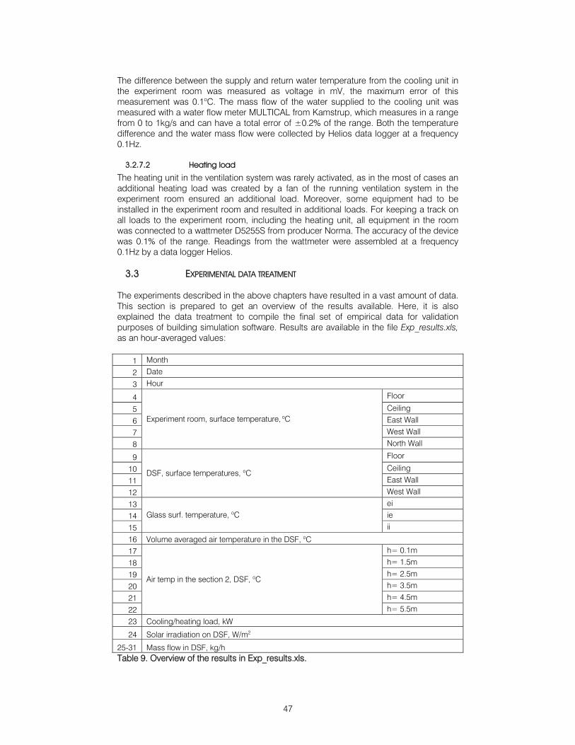
47
The difference between the supply and return water temperature from the cooling unit in the experiment room was measured as voltage in mV, the maximum error of this measurement was 0.1oC. The mass flow of the water supplied to the cooling unit was measured with a water flow meter MULTICAL from Kamstrup, which measures in a range from 0 to 1kg/s and can have a total error of ±0.2% of the range. Both the temperature difference and the water mass flow were collected by Helios data logger at a frequency 0.1Hz.
3.2.7.2 Heating load
The heating unit in the ventilation system was rarely activated, as in the most of cases an additional heating load was created by a fan of the running ventilation system in the experiment room ensured an additional load. Moreover, some equipment had to be installed in the experiment room and resulted in additional loads. For keeping a track on all loads to the experiment room, including the heating unit, all equipment in the room was connected to a wattmeter D5255S from producer Norma. The accuracy of the device was 0.1% of the range. Readings from the wattmeter were assembled at a frequency 0.1Hz by a data logger Helios.
3.3 EXPERIMENTAL DATA TREATMENT
The experiments described in the above chapters have resulted in a vast amount of data. This section is prepared to get an overview of the results available. Here, it is also explained the data treatment to compile the final set of empirical data for validation purposes of building simulation software. Results are available in the file Exp_results.xls, as an hour-averaged values:
1 Month
2 Date
3 Hour
4 Floor
5 Ceiling
6 East Wall
7 West Wall
8
Experiment room, surface temperature, oC
North Wall
9 Floor
10 Ceiling
11 East Wall
12
DSF, surface temperatures, oC
West Wall
13 ei
14 ie
15
Glass surf. temperature, oC ii
16 Volume averaged air temperature in the DSF, oC 17 h= 0.1m
18 h= 1.5m
19 h= 2.5m
20 h= 3.5m
21 h= 4.5m
22
Air temp in the section 2, DSF, oC
h= 5.5m
23 Cooling/heating load, kW
24 Solar irradiation on DSF, W/m2
25-31 Mass flow in DSF, kg/h Table 9. Overview of the results in Exp_results.xls.
48
The surface temperatures in the experiment room are given as an average value for all measurement points on a surface. A great care must be taken when using these values for the validations, as in the periods with the solar radiation a part of the surface is lighted and will have higher temperature than the surfaces in the shadow. Therefore the authors advise not to use this parameter for validation, but only for evaluation of thermal conditions in the room. Surface temperatures in the DSF were measured only in the center-point of each surface and the results of these measurements are available in the file. Please note, that the measurement of the floor surface temperature may be inaccurate as explained in the earlier chapters. Glass surface temperature was measured in the center of the pane, in every big window (6 measurement points). According to the studies of the experimental results the surface temperature of the glazing was nearly identical for the corresponding glass surfaces. In view of that, an average value for all corresponding surfaces is reported as the main result (average for ei-, average for ie-, average for ii-surfaces). Volume averaged air temperature is calculated for the section 2 of the DSF, using measurements of the air temperature gradient in the cavity at 6 heights above the floor. Results for the section 2 of the DSF cavity are used as representative for the whole cavity, as according to studies of experimental data, the temperature gradient existed the same in all three sections of the cavity. Cooling load in the experiment room is calculated according to Equation 3-1. Equation 3-1
tcmQ pc Δ⋅⋅=•
Where, Qc - cooling load, kW •
m - water mass flow rate, kg/s cp - thermal heat capacity of the water, kJ/kgoK Δt - temperature difference of the supply and return water, oK Equation 3-2
hchc QQQ +=,
Where, Qc, h - cooling/heating load to the experiment room, kW Qc - cooling load to the experiment room, kW Qh - heating load to the experiment room, kW The cooling system was activated for the most of the time, as the equipment in the experiment room had a significant contribution to the thermal balance of the room in a form additional heat load. This contribution was measured with the Wattmeter and has been removed from the experimental data set as described in the Equation 3-2. In this equation the cooling load is always negative and heating load is always positive, so the sign of the cooling/heating load in the data file tells whether the cooling or heating power has been delivered to the room to keep the air temperature constant to a given value. Solar irradiation on the external surface of DSF was measured and included into the set of experimental results.

49
The air flow rate was measured in the DSF cavity, this was then converted to the mass flow rate, using the atmospheric pressure, volume averaged air temperature in the cavity and outdoor air relative humidity.
50
REFERENCES
By og Byg (2002) By og Byg, 2002 : Andersen, K T, Heiselberg, P K, Aggerholm, S.
/ Naturlig ventilation i erhvervsbygninger : beregning og dimensionering. Kbh. :. 118 s.
Erell, et al. (2005) Erell, E, Leal, V, and Maldonado, E. 2005, Measurement of air temperature in the presence of a large radiant flux: an assessment of passively ventilated thermometer screens, Boundary-Layer Meteorology, vol. 114, pp. 205-231.
Etheridge (1996) Etheridge, D. 1996. Building ventilation: theory and measurement. - Chichester : John Wiley, 1996. - 724 s.
EN13182 European Standard EN 13182, Ventilation for buildings - Instrumentation requirements for air velocity measurements in ventilated spaces, CEN 2002
Hitchin & Wilson (1967) Hitchin, E R and Wilson, C B. 1967. A review of experimental techniques for the investigation of natural ventilation in buildings. Building Sciences Vol. 2 (1967), pp. 59–82.
Kalyanova & Heiselberg (2007) Kalyanova, O and Heiselberg, P. 2007. Empirical Test Case Specification: Test Cases DSF100_e and DSF200_e : IEA ECBCS Annex43/SHC Task 34 : Validation of Building Energy Simulation Tools. Aalborg: Aalborg University : Department of Civil Engineering. ISSN 1901-726X DCE Tiechnical Report No.033
Larsen (2006) Larsen, T S. 2006. Natural Ventilation Driven by Wind and Temperature Difference. Ph.D Thesis. Aalborg : Department of Civil Engineering : Aalborg University, 2006. 140 p.
Loncour, et al. (2004) Loncour, X, Deneyer, A, Blasco, et al. 2004. Ventilated Double Facades. Classification & Illustration of façade concepts. Belgian Building Research Institute: Department of Building Physics, Indoor Climate & Building Services. October 2004. http://www.bbri.be/activefacades/new/index.cfm?cat=7_documents&sub=1_download
Sonne, et al. (1993) Sonne, J K, Vieira, R K, and Rudd, A F. 1993. Limiting solar radiation effects on outdoor air temperature measurements, ASHRAE Transactions, vol. 99 (I), pp. 231-240.
McWilliams (2002) McWilliams J., (2002). Review of Airflow Measurement Techniques. Lawrence Berkeley National Laboratory, December 1, 2002

1
APPENDIX

2
Detailed plan and section of the test facility, ‘the Cube
1
1
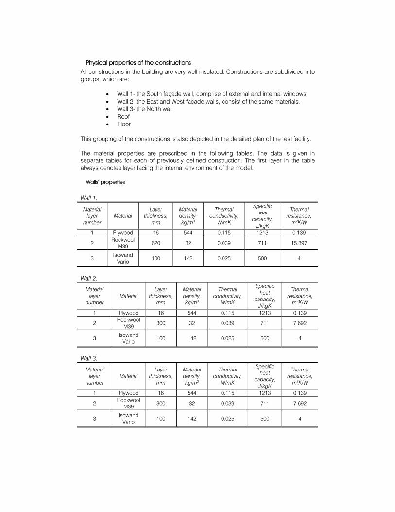
Physical properties of the constructions All constructions in the building are very well insulated. Constructions are subdivided into groups, which are:
• Wall 1- the South façade wall, comprise of external and internal windows • Wall 2- the East and West façade walls, consist of the same materials. • Wall 3- the North wall • Roof • Floor
This grouping of the constructions is also depicted in the detailed plan of the test facility. The material properties are prescribed in the following tables. The data is given in separate tables for each of previously defined construction. The first layer in the table always denotes layer facing the internal environment of the model.
Walls’ properties
Wall 1:
Material layer
number Material
Layer thickness,
mm
Material density, kg/m3
Thermal conductivity,
W/mK
Specific heat
capacity, J/kgK
Thermal resistance,
m2K/W
1 Plywood 16 544 0.115 1213 0.139
2 Rockwool M39
620 32 0.039 711 15.897
3 Isowand
Vario 100 142 0.025 500 4
Wall 2:
Material layer
number Material
Layer thickness,
mm
Material density, kg/m3
Thermal conductivity,
W/mK
Specific heat
capacity, J/kgK
Thermal resistance,
m2K/W
1 Plywood 16 544 0.115 1213 0.139
2 Rockwool M39
300 32 0.039 711 7.692
3 Isowand Vario 100 142 0.025 500 4
Wall 3:
Material layer
number Material
Layer thickness,
mm
Material density, kg/m3
Thermal conductivity,
W/mK
Specific heat
capacity, J/kgK
Thermal resistance,
m2K/W
1 Plywood 16 544 0.115 1213 0.139
2 Rockwool M39
300 32 0.039 711 7.692
3 Isowand Vario
100 142 0.025 500 4
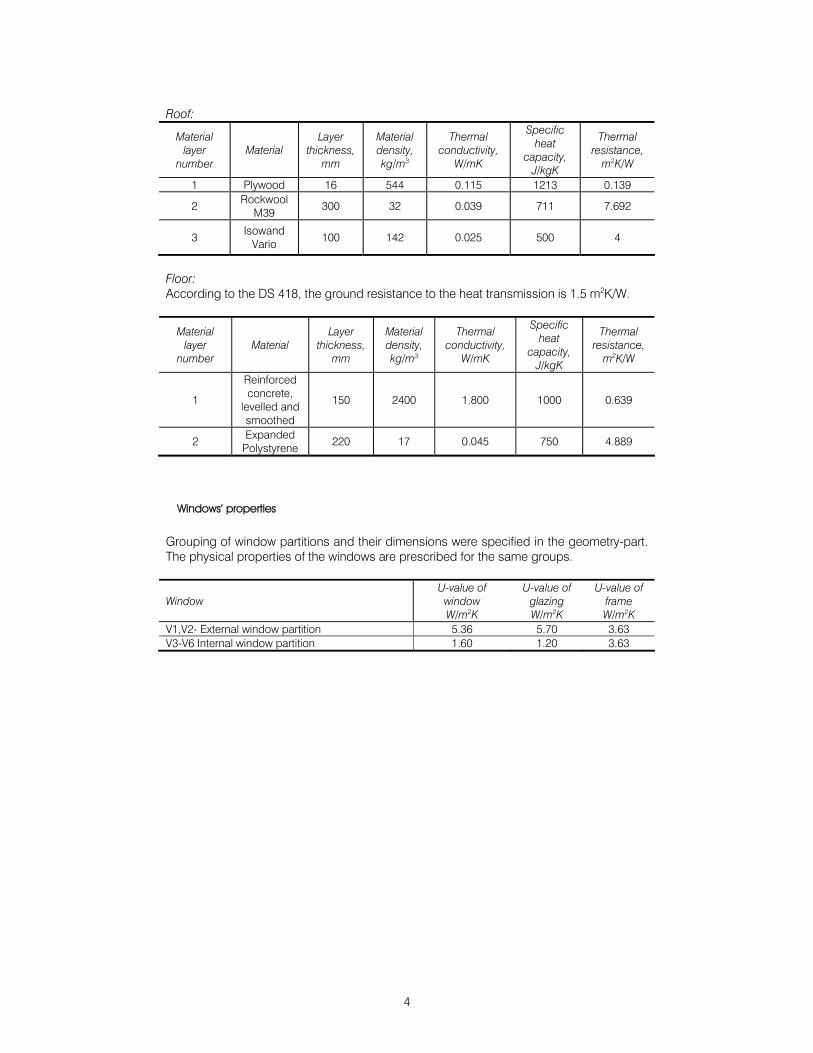
4
Roof:
Material layer
number Material
Layer thickness,
mm
Material density, kg/m3
Thermal conductivity,
W/mK
Specific heat
capacity, J/kgK
Thermal resistance,
m2K/W
1 Plywood 16 544 0.115 1213 0.139
2 Rockwool M39
300 32 0.039 711 7.692
3 Isowand
Vario 100 142 0.025 500 4
Floor: According to the DS 418, the ground resistance to the heat transmission is 1.5 m2K/W.
Material layer
number Material
Layer thickness,
mm
Material density, kg/m3
Thermal conductivity,
W/mK
Specific heat
capacity, J/kgK
Thermal resistance,
m2K/W
1
Reinforced concrete,
levelled and smoothed
150 2400 1.800 1000 0.639
2 Expanded Polystyrene
220 17 0.045 750 4.889
Windows’ properties
Grouping of window partitions and their dimensions were specified in the geometry-part. The physical properties of the windows are prescribed for the same groups.
Window U-value of
window W/m2K
U-value of glazing W/m2K
U-value of frame W/m2K
V1,V2- External window partition 5.36 5.70 3.63 V3-V6 Internal window partition 1.60 1.20 3.63
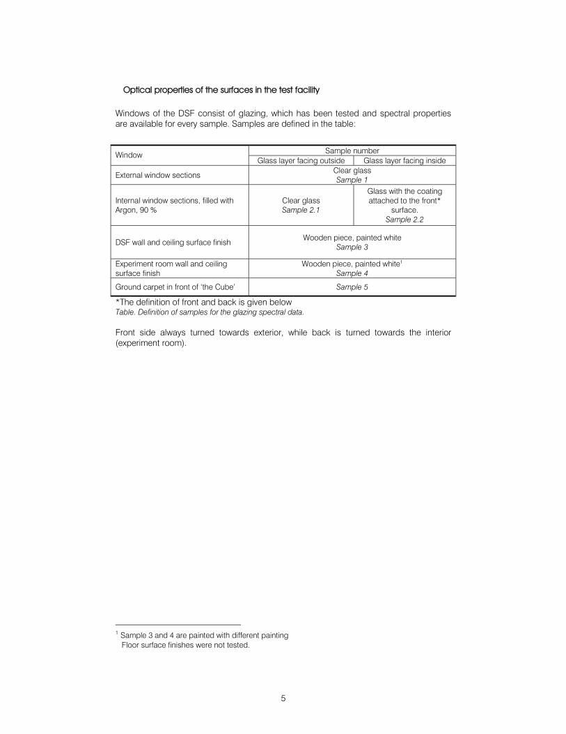
5
Optical properties of the surfaces in the test facility Windows of the DSF consist of glazing, which has been tested and spectral properties are available for every sample. Samples are defined in the table:
*The definition of front and back is given below Table. Definition of samples for the glazing spectral data. Front side always turned towards exterior, while back is turned towards the interior (experiment room).
1 Sample 3 and 4 are painted with different painting Floor surface finishes were not tested.
Sample number Window Glass layer facing outside Glass layer facing inside
External window sections Clear glass Sample 1
Internal window sections, filled with Argon, 90 %
Clear glass Sample 2.1
Glass with the coating attached to the front*
surface. Sample 2.2
DSF wall and ceiling surface finish Wooden piece, painted white
Sample 3
Experiment room wall and ceiling surface finish
Wooden piece, painted white1 Sample 4
Ground carpet in front of ‘the Cube’ Sample 5
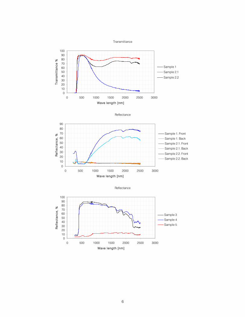
6
Transmittance
0102030405060708090
100
0 500 1000 1500 2000 2500 3000
Wave length [nm]
Tra
nsm
itta
nc
e %
Sample 1
Sample 2.1
Sample 2.2
Reflectance
0
10
20
30
4050
60
70
80
90
0 500 1000 1500 2000 2500 3000
Wave length [nm]
Re
fle
cta
nc
e,
% Sample 1. Front
Sample 1. Back
Sample 2.1. Front
Sample 2.1. Back
Sample 2.2. Front
Sample 2.2. Back
Reflectance
0102030405060708090
100
0 500 1000 1500 2000 2500 3000
Wave length [nm]
Re
fle
cta
nc
e,
%
Sample 3
Sample 4
Sample 5

7

8
ISSN 1901-726X DCE Technical Report No. 030