Embed Size (px)
Citation preview

i
EXPERIMENTAL STUDY ON THE EFFECTS OF NOSE GEOMETRY ON DRAG
OVER AXISYMMETRIC BODIES IN SUPERSONIC FLOW
by
B. TYLER BROOKER
SEMIH M. OLCMEN, COMMITTEE CHAIR
JOHN BAKER
KEITH A. WILLIAMS
A THESIS
Submitted in partial fulfillment of the requirements
for the degree of Master of Science in Aerospace Engineering and Mechanics in
the Department of Aerospace Engineering and Mechanics
in the Graduate School of
The University of Alabama
TUSCALOOSA, ALABAMA
2014

i
Copyright B. Tyler Brooker 2014
ALL RIGHTS RESERVED

ii
ABSTRACT
A new nose shape that was determined using the penetration mechanics to have the
least penetration drag has been tested in the supersonic wind tunnel of The University of
Alabama to determine the aerodynamic characteristics of this nose shape. The aerodynamic
drag measured on the new nose shape and on four additional nose shapes are compared to
each other. The results show that the new nose shape has the least aerodynamic drag. The
measurements were made at Mach numbers ranging from 1.85 to 3.1. This study also
required the maintenance of several components of the University of Alabama’s 6” by 6”
supersonic wind tunnel and modification of the existing data acquisition programs. These
repairs and modifications included the repair and recalibration of the supersonic wind
tunnel, repair of the four-component force balance, and the modification of the tunnel’s
control program.

iii
LIST OF ABBREVIATIONS AND SYMBOLS
a Nose Radius at the base (m)
b Nose Length (m)
CD Drag Coefficient
CPD Penetration-Drag Coefficient
CP Coefficient of Pressure
dmax Maximum Difference from Mean of Experimental Measurements
D Aerodynamic Drag
DP Penetration Drag
ID Intermediate step in defining the nose factor
M Mach Number
N Nose Factor
NF Normalized Force Coefficient
P0 Stagnation Pressure in the Plenum Chamber
P∞ Static Pressure in the Test Section
q∞ Dynamic Pressure
q∞P Dynamic Pressure during penetration
S Cross Sectional Area of Nose Shape Base
x Nose Profile Abscissa (m)
y Nose Profile Ordinate (m), Function describing nose geometry
y’ Local Slope of the nose shape
iv
z Nose Geometry Non-dimensional Ordinate, z=y/a
z’ Slope of the line segment between two adjacent points of the nose shape
α Aspect ratio; Nose radius at the base/ nose length, α=b/a
γ Specific Heat Ratio, 1.4 for air
δ Surface Angle of the Body of Revolution with respect to the Symmetry
Axis along the Direction of the Approach Flow.
ξ Nose Geometry Non-dimensional Abscissa, ξ=x/b
σ Standard Deviation or Uncertainty

v
ACKNOWLEDGMENTS
I would first like to thank advisor, Dr. Semih M. Olcmen, for his guidance and
support through the research for this thesis. I also would like to thank Dr. John Baker and
Dr. Keith A. Williams for serving on my thesis committee. For helping me to diagnose and
repair the tunnel, I would like to thank Dr. Cameron Nott. I would like to thank Mr. Tim
Connell and Sam Tingle for helping to disassemble parts of the tunnel and advice on
restoring worn pieces. I am thankful for the support and encouragement of my family and
loved ones through this experience.
vi
TABLE OF CONTENTS
ABSTRACT …………………………………………………………………..………......ii
LIST OF ABBREVIATIONS AND SYMBOLS …...…………...………………………iii
ACKNOWLEDGMENTS ………………………………………………………………..v
LIST OF TABLES ……………………………………………..……………………….viii
LIST OF FIGURES ...……………………………………………………….……………ix
CHAPTER 1 – INTRODUCTION AND HISTORICAL BACKGROUND ….…………..1
1.1. Introduction ………………………………….……………………….1
1.2. Historical Background of Nose Shape Design ……………………….2
CHAPTER 2 - NOSE SHAPE DESIGN PROCEDURE ….….……………………….….7
2.1. Nose Factor …………………………………..…………………….…7
2.2. Calculation of the New Nose Shape …..……..…………………….…9
2.3. Description of Nose Geometries …..…..……..……………………...11
CHAPTER 3 - EXPERIMENTAL SETUP ……..…………………………….…………13
3.1. Supersonic Wind Tunnel …………..…..……..……………………...13
3.2. Four Component Force Balance …..……..………………..………...18
3.3. Schlieren System ………………………...………………..………...19
3.4. Manufactured Nose Shapes …………………………………….…...20
CHAPTER 4 - RESULTS AND DISCUSSION ..…………………………….…………22
4.1. Drag Measurement Method …………………………………….…...22
4.2. Drag Coefficient Results ……………….……………………….…...26
vii
CHAPTER 5 – CONCLUSIONS AND FUTURE WORK ….………………….…….…33
REFERENCES ………………...…………………………….………………….…….…35
APPENDIX A - TUNNEL LAB MODIFICATIONS ………………….…......…………37
A1. Tunnel Maintenance and Repairs ……………………………………37
A2. Force Balance Repairs and Modifications ……..……………………38
A3. Tunnel Control Program Modifications ………..……………………42
APPENDIX B - 6-INCH X 6-INCH TUNNEL OPERATION …….….……...…………44
B1. Filling the Storage Tank ………..……………………………………44
B2. Pre-Run Checks ………………..……………………………………46
B3. Program for Tunnel Operation ….…………...………………………47
B4. Troubleshooting ………………..……………………………………49
B5. Conclusion ……………………..……………………………………52
APPENDIX C - TUNNEL RUN DATA ……….………….………………….…………53
C1. Schlieren Images of Tunnel Runs ...…….……………………….…...53
C2. Tunnel Run Data ...…….………………………………….…….…...55
viii
LIST OF TABLES
2.3.1: Nose shape equations and N values ……………….……..……..…...………....…..12
3.1.1: Calibration Results for Tunnel with object in test section ….….………….............17
4.2.1: Strain Measurements and Uncertainty on Cone Shape …..……………..................27
4.2.2: Force Measurements and Uncertainty on Cone Shape …………………………....27
4.2.3: Plenum Pressure Measurements and Uncertainty on Cone Shape…...……….........28
4.2.4: Base Drag Values found using Cone Shape ……………………..………..…....….29
4.2.5: Ogive Shape Experimental Values …………………………………..…..………..30
4.2.6: ¾ Power Shape Experimental Values ……………………...……………...………30
4.2.7: Jones’s Shape Experimental Values ……………………………………………....30
4.2.8: New Shape Experimental Values …………………………………………….…....31
B4.1: Tunnel Troubleshooting Guide: …………………………………………………...49
ix
LIST OF FIGURES
2.2.1: Nose shape presented with line segments ….…………………..…………………...9
2.3.1: Two-Dimensional Nose Geometries ………………………………..……………..12
3.1.1: Schematic of the Supersonic wind tunnel lab ……………………………………...13
3.1.2: Mass Flow Rate Control Instrumentation and Data Acquisition Setup………........14
3.1.3: Wedge at Counter Number 1500……………………………................…………..15
3.1.4: Wind Tunnel Calibration …………...……………………………………...….…..16
3.2.1: University of Alabama Four Component Force Balance………...…………...........18
3.2.2: Original Axial Strain Calibration .…………………………………………………19
3.2.3: Force balance on calibration stand ……………...………………...…………….…19
3.3.1: University of Alabama Schlieren System Setup ……………………...……….…..20
3.4.1: Models used in Drag Testing ….….….………….………………...……………....21
4.1.1: Graph of Axial Strain alongside Plenum Pressure ……………………..…...…......23
4.1.2: Example of Axial Strain Readings after balance modifications were made .….......24
4.1.3: New Axial Strain Calibration …………………………………………..…...…......24
4.1.4: Figure Describing Principle of Shock Waves Inside Tunnel …………...………….25
4.2.1: Historical Drag Coefficient Data……….....…………...……………………..……29
4.2.2: Corrected Drag Coefficient Values …………………………...…………..……….31
4.2.3: Drag Coefficient Values Relative to Cone…………………………………………32
4.2.4: Non-Dimensionalized Drag Comparison …………………………………………32
A2.1: Force Balance Strain Gage Locations and Modifications….………………….…...39

x
A2.2: Comparison Between Old Gage and Newly Installed Gage ………..……………..39
A2.3: Full Wheatstone Bridge Configuration …..…….……………….………………....40
A2.4: Current Gage Configuration …………………………………...……...…………..40
A2.5: Insulation applied to the inside and outside of the force balance ...………………..41
B1.1: Wind Tunnel Power Switch ……………………………………………………….44
B1.2: Compressor Control Panel ..……………………………………………………….45
B1.3: Dehumidifier Control Panel…..………………………………...……………..…...45
B2.1: Tunnel region behind the test section and rear plate knob ………...……..…….…...47
B3.1: Tunnel Run Program ……..………...…...…………………………………………48
B4.1: MoveValve.vi ………………….…………………..…...…………………………51
B4.2: Manual Valve Operation Location ………………..……………...….…………….51
C1.1-C1.3: Calibration Wedge at Various Counter Numbers …………………………...53
C1.4-C1.10: Test Models at Various Counter Numbers …...……………….……………53
C2.1-C2.54: Run Data from Test Models at Various Counter Numbers …………..….….55
1
CHAPTER 1
INTRODUCTION AND HISTORICAL BACKGROUND
1.1 Introduction
Supersonic travel poses many problems on missiles and rockets designed to produce
maximum range and penetration into a target. In an effort to increase the efficiency of rocket
designs a variety of nose shapes have been developed. This thesis will discuss the design of an
optimized nose shape for minimum penetration drag. This design is tested using the University of
Alabama’s supersonic wind tunnel and compared to shapes currently being utilized by the
aerospace industry.
The effect of nose geometry on penetration performance has been studied for decades. A
variety of analytical methods have been performed to attempt to optimize the nose shape for a
penetrator. The new shape design was created by dividing the nose shape into line segments and
searching through numerical space for the combination of line segment slopes that produced the
nose geometry with the lowest nose shape factor. This nose shape factor is derived using
penetration mechanics theory. The new design should provide an updated perspective on nose
shape design.
The experimental data is collected in the 6” x 6” supersonic wind tunnel at Mach numbers
between 2.5 and 3.6. This tunnel is a blowdown type supersonic tunnel that uses a 1000 cubic foot
storage tank to hold pressurized air that is released into the plenum chamber of the supersonic
tunnel. The pressure in the plenum chamber is maintained at a constant value in order to provide
a constant static pressure in the test section of the wind tunnel. A tunnel program was developed
2
to automate the run of the supersonic tunnel by Daniel Lewis as part of his master’s thesis [Lewis,
2006]. This program controls the pneumatic valve that maintains a consistent running procedure.
A four component force balance is used to measure the drag on the nose shapes. The use
of the force balance unit to collect the drag data required modifications to be made to the tunnel
control program and to the force balance strain gage configuration. More details on these
modifications can be found in Appendix A. In the current work, only the axial force gages and a
temperature compensation gage were used. The temperature gage was used to ensure there was
minimal effect on the strain readings due to the temperature changes from the total pressure loss
during the tunnel run.
1.2 Historical Background of Nose Shape Design
Nose shape geometry has been a topic discussed for more than a century. Jean-Victor
Poncelet introduced modern analytical penetration mechanics when he studied velocity dependent
pressure action on a spherical cannon ball [Poncelet, 1829]. Variants of this work are still used
today to estimate penetration depth of a projectile. The geometry of a nose is critical to an object’s
penetration mechanics and its aerodynamic characteristics. As an employee of the Armament
Research Department in the British army, Hill began researching the influence of “headshape” in
penetration of thick armor [Hill, 1980]. This research culminated in a paper where he discussed a
phenomenon he termed “cavitation” that was responsible for the degradation of a penetrators
performance [Hill, 1980]. A few years later, Forrestal related the nose factor, N, with the
performance of a rigid penetrator [Forrestal, 1986, 1991, 1992]. Here at the University of Alabama,
Dr. Stanley Jones calculated the nose factor for several axisymmetric geometries and used calculus
of variations to propose a simple approximate analytical geometry to minimize the nose factor
3
[Jones, 1998]. The result was a blunt tipped nose and resembles a similar design proposed by
Eggers [Eggers, 1957].
Yefremov and Takovitskii used the Euler equations to design nose shapes with specified
dimensions and volumes and minimal aerodynamic wave drag [Yefremov, 2006]. At Mach
numbers of 2 and 4 and with aspect ratios (AR= nose length divided by nose radius at the base),
b/a=4 and b/a=8, the optimal shape of their nose are blunt with surfaces perpendicular to incoming
flow. When removing the volume restriction, the resulting shape is very similar to the shape
defined by Jones [Jones, 1998]. This is significant because the two methods differ from each other.
The analysis made by Yefremov minimized aerodynamic drag while the analysis made by Jones
was focused on minimizing penetration drag. The similarity is not surprising since both groups use
Newton’s theory in describing the pressure distribution over the body; however, the resulting
similarity of the shapes suggests a strong correlation between aerodynamic drag and the shapes
penetration mechanics.
Takovitskii discussed another procedure for determining an optimal nose shape using a
step-by-step construction of the segments of the shapes with minimum aerodynamic wave drag
based on the locally extremal generatrix defined for different aspect ratio noses under different
free-stream Mach number conditions. His results also show a seemingly blunt nose, where the first
segment makes an angle of approximately 55° with respect to the nose centerline [Takovitskii,
2006a]. He also published a paper detailing an analytical method to minimize the aerodynamic
wave drag with results that indicate an optimal shape that follows the two-thirds power law
[Takovitskii, 2006b].
Foster and Dulikravich [1997] used two methods to compare and contrast their
performance on optimization of nose shape geometry. The two methods were a hybrid gradient
4
optimization method and a hybrid genetic optimization method, and were used to evaluate optimal
shapes of both a star shaped axisymmetric body and a three-dimensional lifting body at a zero
degree angle-of-attack. The results for the star shaped axisymmetric nose optimized for minimum
aerodynamic drag had a short, pointed nose section with a base diameter much smaller than the aft
section diameter [Foster, 1997].
Taking into consideration the aerodynamic drag, heat transfer, and payload volume, Lee et
al. [2006] obtained an optimal nose shape for a space launcher through the use of a multipoint
response surface design method. They began with a baseline shape and focused on performance
of three design criteria; maximum drag coefficient, maximum dynamic pressure, and first stage
burnout. These design points correspond to Mach numbers of 1.2, 1.8, and 4.6 respectively. Their
optimization yields a 24% improvement of drag performance of the launcher nose shape compared
to the spherically rounded baseline nose (Korean three-staged rocket KSR-III nose). The nose
shape achieved in the optimization was similar to the one proposed by Jones [1998], but had a
more blunt nose [Lee, 2006]. Ragnedda and Serra [2010] obtained similarly blunt shapes using a
particle swarm optimization method.
Through the use of an evolutionary-algorithm optimization and ANSYS CFX
computational fluid dynamics solver, Deepak et al. [2008] optimized the nose-cone shape of a
hypersonic vehicle. For a baseline nose shape, the team used the HyShot experimental hypersonic
flight vehicle, that has been tested jointly with the U.S. and Australian Defense Agencies. The
optimized shape had a 2% drag reduction and utilized a spherically rounded tip followed by the
shape proposed by Jones [1998] until a location of ξ=0.2, and a thicker aft section that followed a
curve between the new optimal nose shape defined later in this thesis and the tangent ogive
[Deepak, 2008].
5
The purpose of the current investigation is to define a new nose shape optimized by
minimizing the nose factor, N, using penetration mechanics theory, and compare the aerodynamic
drag characteristics of this new shape to the drag characteristics of four other common shapes. For
this purpose a new numerical method was introduced to minimize the nose factor, and was
subsequently used to find an optimum nose shape. Next the aerodynamic drag forces for the five
shapes were measured in a supersonic wind tunnel and the drag coefficient values calculated using
the measured drag were compared to each other. The other four shapes in the study were: a three-
quarter power series nose shape, Jones Approximate Minimal Nose Geometry (AMNG), a tangent
ogive, and a conical nose. These four shapes were chosen since they are the commonly encountered
nose shapes, both as penetrators and as aerodynamic bodies of revolution in previous research
[Jones, 1998; Eggers, 1957; Forrestal, 2009]. Measurements made in earlier research at the
University of Alabama by Lewis [2006] were inconclusive due to the marginal difference in drag
coefficients between the nose shapes. In his study Lewis used long noses with an aspect ratio of
b/a = 4 and four shapes: ogive, cone, three-quarter power series nose, and the AMNG. Despite the
marginal differences it seemed as though the AMNG produced the least drag [Lewis, 2006]. In
order to improve the accuracy of this new round of testing, the new shapes were manufactured
with an aspect ratio of b/a = 2. The reason for manufacturing new nose shapes was to increase the
drag for all of the shapes to help differentiating the drag values between different nose shapes.
As a note, this optimization approach was designed to maximize penetration depth. The
process does not take into account any heat transfer effects which may influence the final nose
geometry. The impact of heating on the effective application of the nose shape has not been
considered either.

6
The following sections will detail the various procedures involved in testing the new nose
shape. Chapter 2 discusses the optimization method for developing the new nose shapes and the
penetration mechanics used to develop it. Chapter 3 explains the systems used to test the object,
including the high speed wind tunnel, force balance, and schlieren system. Chapter 4 presents the
results of the study, and includes a discussion of those results. Chapter 5 draws a close to the
research and suggests modifications for further study and experimentation.
7
CHAPTER 2
NOSE SHAPE DESIGN PROCEDURE
The optimization of the nose required understanding of penetration mechanics and the
development of a method to search for a shape that minimized the nose factor of a penetrator. In
this chapter, details on the development of the new nose are presented.
2.1 Nose Factor
The nose factor, N, is a parameter commonly used in penetration mechanics to quantify the
penetration-drag characteristics of a nose geometry during penetration of hard targets. It is a non-
dimensional quantity that is only dependent on the geometry of the nose shape. In penetration
mechanics, it is common to approach the problem by ignoring the friction forces acting on a
penetrator and assume the pressure forces are the primary source of penetration drag. Due to this
assumption, the penetration-drag coefficient also becomes a function independent of everything
except nose geometry. This also causes the nose factor and penetration-drag coefficient to differ
by a constant multiplier. An analysis of the case for pressure-dependent friction has been given by
Jones and Rule [2000], but will not be considered in this study.
The following equations detail the relationship between the nose factor, the penetration
drag coefficient, and the coefficient of pressure, Cp. The coefficient of pressure has been
approximated, using an equation similar to Newton’s theory which applies to hypersonic flows
[Anderson, 2007], to apply to a slender body during penetration. The expression for the 𝐶𝑝 is as
follows:

8
𝐶𝑝 = 2 𝑠𝑖𝑛2𝛿 =2y’2
1+y’2 (2.1.1)
Using this coefficient of pressure, and neglecting the viscous forces, the drag force can be found
using:
𝐷𝑃 = 𝐶𝑃𝐷 ∗ 𝑞∞𝑃 ∗ 𝜋𝑎2 = 2𝜋 ∗ 𝑞∞𝑃 ∫ 𝐶𝑝 ∗ y ∗ y’ ∗ dx𝑏
0 (2.1.2)
To lead to the definition of the nose factor, an intermediate step, ID is defined as a function of the
nose geometry:
𝐼𝐷 =𝐷𝑃
2𝜋∗𝑞∞𝑃= ∫ 𝐶𝑝 ∗ y ∗ y’ ∗ dx
𝑏
0= ∫
2yy’3
1+y’2dx
𝑏
0 (2.1.3)
To further simplify this expression the x and y coordinates are non-dimensionalized with the nose
length, b, and the nose base radius, a, respectively, leading to a new expression for the ID:
𝐼𝐷 = 2𝛼2𝑎2 ∫zz’3
1+𝛼2z’2dξ
1
0 (2.1.4)
Finally the nose factor is defined as:
𝑁 =𝐶𝑃𝐷
2=
𝐼𝐷
𝑎2 = 2𝛼2 ∫zz′3
1+𝛼2z′2 dξ
1
0 (2.1.5)
As was discussed earlier the expression for nose factor is solely dependent on the nose
geometry. This allows the nose factor to be directly related to penetration-drag coefficient and
means the minimum nose factor, N, also corresponds to the nose that would experience the least
resistance during penetration. Once again, it should be emphasized that this penetration-drag
coefficient, CPD, is defined only using the form drag, drag due to the pressure related forces,
without taking into account viscous effects. The penetration-drag coefficient used in penetration
mechanics differs from the drag coefficient, CD, used in fluid mechanics. The aerodynamic drag
coefficient of an object is dependent on Reynolds and Mach numbers [Anderson, 2007]. However
if Newton’s theory, the appropriate values for dynamic pressure, q, and aerodynamic drag
coefficient, CD, is applied, then equation 2.1.2, which describes penetration drag, DP, becomes the

9
equation for aerodynamic drag, D. This leads to the conclusion that minimizing nose factor will
also minimize an object’s aerodynamic drag.
2.2 Calculation of the New Nose Shape
In this study to find a new nose shape for a rigid body penetrator, the nose factor was
optimized. As discussed in section 2.1, a minimum nose factor will correspond to a nose shape
with a minimum penetration-drag coefficient, which would result in a penetrator that would travel
deepest when impacting a target. In order to find the optimum shape with the fewest assumptions,
it was decided that a computer program would be used to solve for the shape using a step-by-step
method. The computer program was designed to search through numerical space to find the nose
shape with the lowest N value by splitting the geometry of the nose into line segments. To
accomplish this, the program first expressed the nose shape using line segments equally spaced
along the longitudinal axis of the nose. This procedure is depicted in Figure 2.2.1. After the shape
is spilt into line segments, the nose factor for each line segment was computed. The program
minimizes the change in N calculated as the sum of the nose factors for each line segment.
Figure 2.2.1: Nose shape presented with line segments
Using Figure 2.2.1, the slope, z’, of a line segment between two adjacent points can be expressed
as:
𝑧′ =𝑧𝑖−𝑧𝑖−1
𝜉𝑖−𝜉𝑖−1 (2.2.1)
𝜉1 𝜉2 𝜉3 𝜉𝑛 𝜉𝑛+1
𝑧𝑛+1 𝑧𝑛 𝑧3
𝑧2 𝜉
𝑧
10
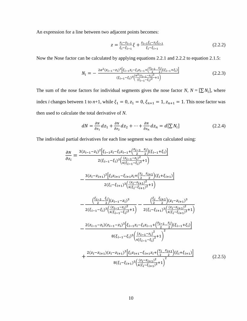
An expression for a line between two adjacent points becomes:
𝑧 =𝑧𝑖−𝑧𝑖−1
𝜉𝑖−𝜉𝑖−1𝜉 +
𝑧𝑖−1𝜉𝑖−𝑧𝑖𝜉𝑖−1
𝜉𝑖−𝜉𝑖−1 (2.2.2)
Now the Nose factor can be calculated by applying equations 2.2.1 and 2.2.2 to equation 2.1.5:
𝑁𝑖 = − 2𝛼2(𝑧𝑖−1−𝑧𝑖)3[𝜉𝑖−1𝑧𝑖−𝜉𝑖𝑧𝑖−1+(
𝑧𝑖−12
−𝑧𝑖2
)(𝜉𝑖−1+𝜉𝑖)]
(𝜉𝑖−1−𝜉𝑖)3(𝛼2(𝑧𝑖−1−𝑧𝑖)2
(𝜉𝑖−1−𝜉𝑖)2 +1) (2.2.3)
The sum of the nose factors for individual segments gives the nose factor N, N = [∑ 𝑁𝑖], where
index i changes between 1 to n+1, while 𝜉1 = 0, 𝑧1 = 0, 𝜉𝑛+1 = 1, 𝑧𝑛+1 = 1. This nose factor was
then used to calculate the total derivative of N.
𝑑𝑁 =𝜕𝑁
𝜕𝑧1𝑑𝑧1 +
𝜕𝑁
𝜕𝑧2𝑑𝑧2 + ⋯ +
𝜕𝑁
𝜕𝑧𝑛𝑑𝑧𝑛 = 𝑑[∑ 𝑁𝑖] (2.2.4)
The individual partial derivatives for each line segment was then calculated using:
𝜕𝑁
𝜕𝑧𝑖=
3(𝑧𝑖−1−𝑧𝑖)2[𝜉𝑖−1𝑧𝑖−𝜉𝑖𝑧𝑖−1+(𝑧𝑖−1
2−
𝑧𝑖2
)(𝜉𝑖−1+𝜉𝑖)]
2(𝜉𝑖−1−𝜉𝑖)3((𝑧𝑖−1−𝑧𝑖)2
4(𝜉𝑖−1−𝜉𝑖)2+1)
−3(𝑧𝑖−𝑧𝑖+1)2[𝜉𝑖𝑧𝑖+1−𝜉𝑖+1𝑧𝑖+(
𝑧𝑖2
−𝑧𝑖+1
2)(𝜉𝑖+𝜉𝑖+1)]
2(𝜉𝑖−𝜉𝑖+1)3((𝑧𝑖−𝑧𝑖+1)2
4(𝜉𝑖−𝜉𝑖+1)2+1)
−(
𝜉𝑖−12
−𝜉𝑖2
)(𝑧𝑖−1−𝑧𝑖)3
2(𝜉𝑖−1−𝜉𝑖)3((𝑧𝑖−1−𝑧𝑖)2
4(𝜉𝑖−1−𝜉𝑖)2+1)−
(𝜉𝑖2
−𝜉𝑖+1
2)(𝑧𝑖−𝑧𝑖+1)3
2(𝜉𝑖−𝜉𝑖+1)3((𝑧𝑖−𝑧𝑖+1)2
4(𝜉𝑖−𝜉𝑖+1)2+1)
−2(𝑧𝑖−1−𝑧𝑖)(𝑧𝑖−1−𝑧𝑖)3[𝜉𝑖−1𝑧𝑖−𝜉𝑖𝑧𝑖−1+(
𝑧𝑖−12
−𝑧𝑖2
)(𝜉𝑖−1+𝜉𝑖)]
8(𝜉𝑖−1−𝜉𝑖)5((𝑧𝑖−1−𝑧𝑖)
2
4(𝜉𝑖−1−𝜉𝑖)2+1)
2
+2(𝑧𝑖−𝑧𝑖+1)(𝑧𝑖−𝑧𝑖+1)3[𝜉𝑖𝑧𝑖+1−𝜉𝑖+1𝑧𝑖+(
𝑧𝑖2
−𝑧𝑖+1
2)(𝜉𝑖+𝜉𝑖+1)]
8(𝜉𝑖−𝜉𝑖+1)5((𝑧𝑖−𝑧𝑖+1)2
4(𝜉𝑖−𝜉𝑖+1)2+1)2 (2.2.5)

11
The new nose shape is defined by updating the 𝑧𝑖 coordinates based on the 𝜕𝑁/(𝜕𝑧𝑖 ) values since
these partial derivatives also show the sensitivity of the N with respect to the 𝑧𝑖 coordinates. Each
𝜕𝑁/(𝜕𝑧𝑖 ) value is used to update the corresponding 𝑧𝑖 value using:
𝑧𝑖,𝑗+1 = 𝑧𝑖,𝑗−𝐶1 ∗ (𝜕𝑁
𝜕𝑧𝑖 )𝑗 (2.2.6)
In this expression C1 is just a constant equal to 0.0001, and indicates an iteration step. Each new
𝑧𝑖 value was immediately used in the successive 𝜕𝑁/(𝜕𝑧𝑖 ) calculation. The program was
initialized with a circular cylindrical rod shaped nose. The length of the nose from 0 to 1 along the
longitudinal domain was divided into 1000 equal segments. The number of segments required was
investigated and it was determined that the solution was independent of iteration steps once more
than 500 segments were used. The program had a specified end condition of ∑𝜕𝑁
𝜕𝑧𝑖 < 1.1 ∗ 10−6.
This condition was set to ensure a converged solution was obtained. Once the solution converges,
the largest change in the 𝑧𝑖 values between the last two iterations is less than 10−10. These 𝑧𝑖
values therefore define our new nose shape. The body shape has almost a flat nose with 𝑧2 =
0.1211. The shape is similar to the one previously presented by Jones with a slightly more blunt
tip [Jones, 1998]. When the program was ran with various aspect ratio values, it indicated that the
nose shape does not change with α. The limiting value of the nose factor calculated for the first
segment, lim𝑥2→0
𝑁2 = 𝑧22 indicates a lower limit that can be achieved for the nose factor.
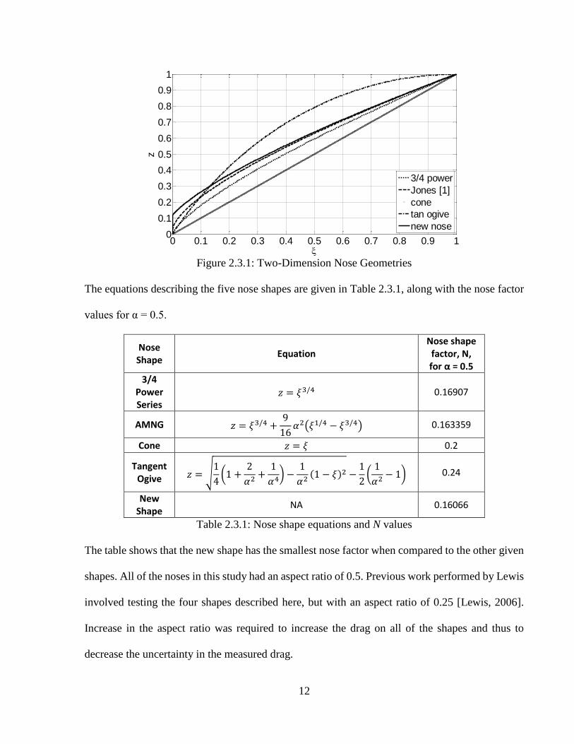
2.3 Description of Nose Geometries
The nose shapes tested in this study were a three-quarter power series nose, Approximate
Minimal Nose Geometry, a standard cone, a tangent ogive, and the newly defined nose. Figure
2.3.1 shows a two-dimensional plot of the nose geometries for comparison.
12
Figure 2.3.1: Two-Dimension Nose Geometries
The equations describing the five nose shapes are given in Table 2.3.1, along with the nose factor
values for α = 0.5.
Nose Shape
Equation Nose shape
factor, N, for α = 0.5
3/4 Power Series
𝑧 = 𝜉3/4 0.16907
AMNG 𝑧 = 𝜉3/4 +9
16𝛼2(𝜉1/4 − 𝜉3/4) 0.163359
Cone 𝑧 = 𝜉 0.2
Tangent Ogive 𝑧 = √
1
4(1 +
2
𝛼2+
1
𝛼4) −
1
𝛼2(1 − 𝜉)2 −
1
2(
1
𝛼2− 1) 0.24
New Shape
NA 0.16066
Table 2.3.1: Nose shape equations and N values
The table shows that the new shape has the smallest nose factor when compared to the other given
shapes. All of the noses in this study had an aspect ratio of 0.5. Previous work performed by Lewis
involved testing the four shapes described here, but with an aspect ratio of 0.25 [Lewis, 2006].
Increase in the aspect ratio was required to increase the drag on all of the shapes and thus to
decrease the uncertainty in the measured drag.
0 0.1 0.2 0.3 0.4 0.5 0.6 0.7 0.8 0.9 10
0.1
0.2
0.3
0.4
0.5
0.6
0.7
0.8
0.9
1
z
3/4 power
Jones [1]
cone
tan ogive
new nose
13
CHAPTER 3
EXPERIMENTAL SETUP
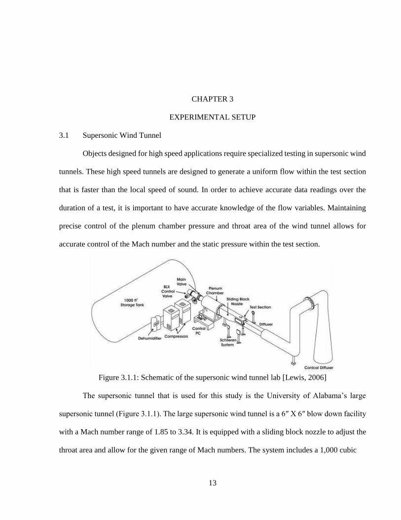
3.1 Supersonic Wind Tunnel
Objects designed for high speed applications require specialized testing in supersonic wind
tunnels. These high speed tunnels are designed to generate a uniform flow within the test section
that is faster than the local speed of sound. In order to achieve accurate data readings over the
duration of a test, it is important to have accurate knowledge of the flow variables. Maintaining
precise control of the plenum chamber pressure and throat area of the wind tunnel allows for
accurate control of the Mach number and the static pressure within the test section.
Figure 3.1.1: Schematic of the supersonic wind tunnel lab [Lewis, 2006]
The supersonic tunnel that is used for this study is the University of Alabama’s large
supersonic tunnel (Figure 3.1.1). The large supersonic wind tunnel is a 6″ X 6″ blow down facility
with a Mach number range of 1.85 to 3.34. It is equipped with a sliding block nozzle to adjust the
throat area and allow for the given range of Mach numbers. The system includes a 1,000 cubic
14
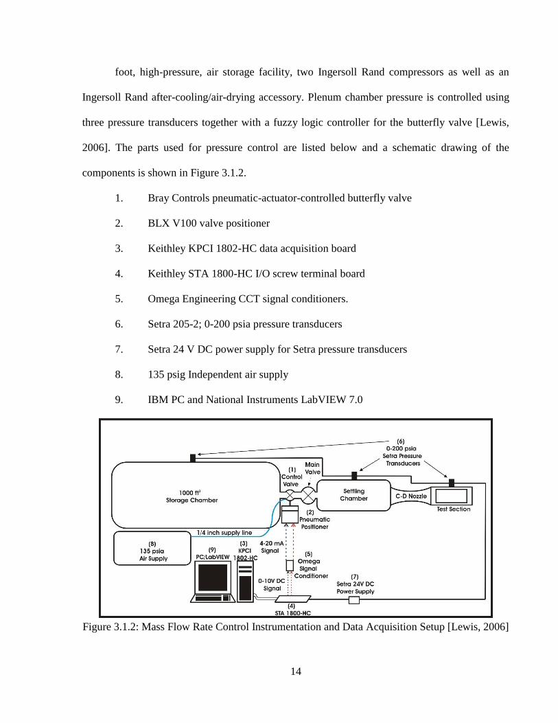
foot, high-pressure, air storage facility, two Ingersoll Rand compressors as well as an
Ingersoll Rand after-cooling/air-drying accessory. Plenum chamber pressure is controlled using
three pressure transducers together with a fuzzy logic controller for the butterfly valve [Lewis,
2006]. The parts used for pressure control are listed below and a schematic drawing of the
components is shown in Figure 3.1.2.
1. Bray Controls pneumatic-actuator-controlled butterfly valve
2. BLX V100 valve positioner
3. Keithley KPCI 1802-HC data acquisition board
4. Keithley STA 1800-HC I/O screw terminal board
5. Omega Engineering CCT signal conditioners.
6. Setra 205-2; 0-200 psia pressure transducers
7. Setra 24 V DC power supply for Setra pressure transducers
8. 135 psig Independent air supply
9. IBM PC and National Instruments LabVIEW 7.0
Figure 3.1.2: Mass Flow Rate Control Instrumentation and Data Acquisition Setup [Lewis, 2006]
15
The tunnel was last calibrated in 2006 when Lewis reworked the control program to automate the
tunnel runs. The calibration was used to determine the relation between the counter number that is
used to determine the location of the sliding bottom wall and the Mach number in the tunnel. The
bottom wall of the tunnel is actuated using a motor/worm-gear mechanism. The calibration was
performed using two methods. The first technique used to calculate the Mach number in the test
section was to measure the shock angles on a two-dimensional wedge at several throat settings.
The schlieren system was used to visualize the flow over the wedge which allowed the shock
angles to be measured. Lewis determined that the lowest possible counter number setting of 0004
resulted in a Mach number of 1.75. The highest setting was a counter number of 2500 and resulted
in a Mach number of 3.65 [Lewis, 2006]. While this method is a simple way to check the Mach
number of the tunnel, it can be inaccurate due to difficulty in measuring the shock-wave angle
using the schlieren pictures. In addition, asymmetric geometry of the tunnel wall results in non-
symmetric boundary layer development on the bottom and the top walls of the tunnel making the
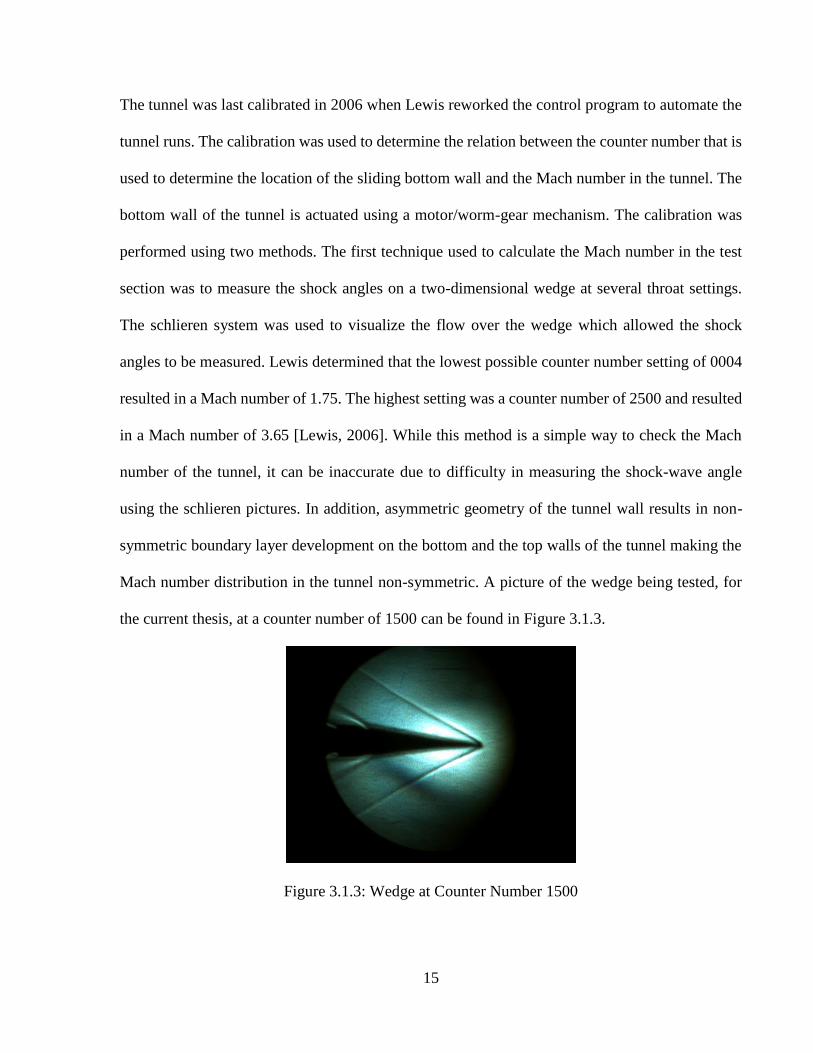
Mach number distribution in the tunnel non-symmetric. A picture of the wedge being tested, for
the current thesis, at a counter number of 1500 can be found in Figure 3.1.3.
Figure 3.1.3: Wedge at Counter Number 1500
16
In order to insure the accuracy of the wind tunnel calibration, Lewis also conducted a
calibration based on normal shock relations. A pressure rake equipped with nine Pitot probes was
designed and built for that purpose. The Pitot pressures and velocities were measured at a variety
of throat settings, but the tunnel was unable to start at the extreme throat settings below 1500 and
above 2250 due to the size and of the pressure rake inside the tunnel. The pressure rake showed a
variance in Mach number near the walls of the tunnel, especially at the bottom wall, but confirmed
that the center of the test section was at a uniform Mach number [Lewis, 2006]. This calibration is
more accurate and insensitive to flow irregularity, but is more intensive and not functional for all
throat settings.
During the current research it was found that the sliding block of the tunnel could no longer
be moved to a location corresponding to a counter number setting below 0435. To ensure the
counter had not shifted since the last calibration, the tunnel needed to be recalibrated. It was
decided that a calibration using the two-dimensional wedge technique would be sufficient to
confirm that calibration already made by Lewis was still valid or if the counter number had shifted.
Since the tunnel has not been modified in any way since the last calibration this method was
deemed sufficient in determining whether the counter has shifted or if the bottom sliding block
was jammed preventing the tunnel to run at low Mach number settings. It was decided that if the
counter had shifted then the calibration made by Lewis could still be used with new counter
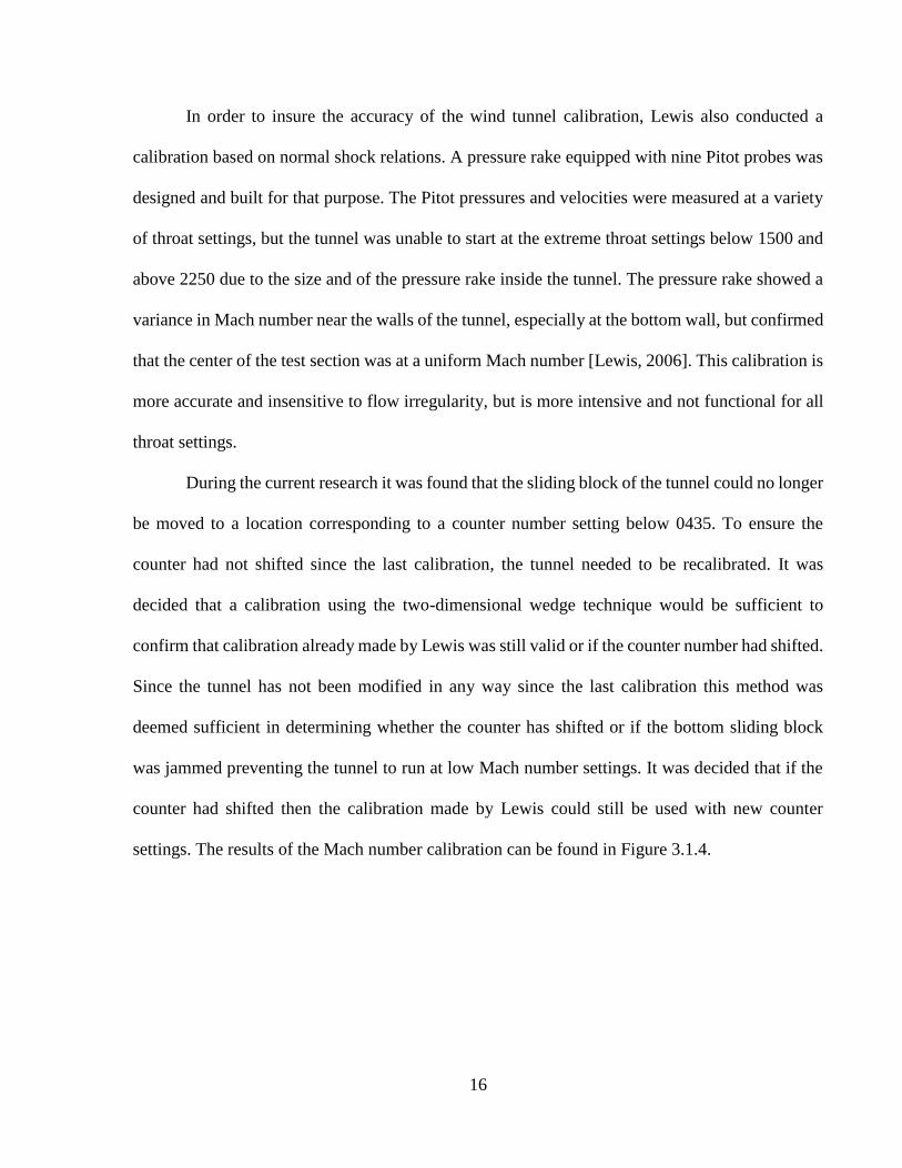
settings. The results of the Mach number calibration can be found in Figure 3.1.4.
17
Figure 3.1.4: Wind Tunnel Calibration
The results of the calibration show that the tunnels counter number has shifted slightly
since the last calibration. By moving the old calibration up by 0300 on the counter setting the
calibration realigns with the results of the new wedge calibration. The starting pressures were also
recalculated using a similar method. To conduct the tests properly, both of the counter values
corresponding to different tunnel Mach numbers and the corresponding starting plenum chamber
pressure values need to be available when running the tunnel. A new sheet outlining the common
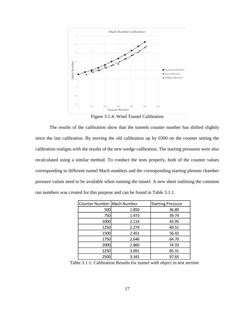
run numbers was created for this purpose and can be found in Table 3.1.1.
Table 3.1.1: Calibration Results for tunnel with object in test section
Counter Number Mach Number Starting Pressure
500 1.850 36.89
750 1.973 39.74
1000 2.114 43.95
1250 2.274 49.51
1500 2.451 56.42
1750 2.646 64.70
2000 2.860 74.33
2250 3.091 85.31
2500 3.341 97.65
18
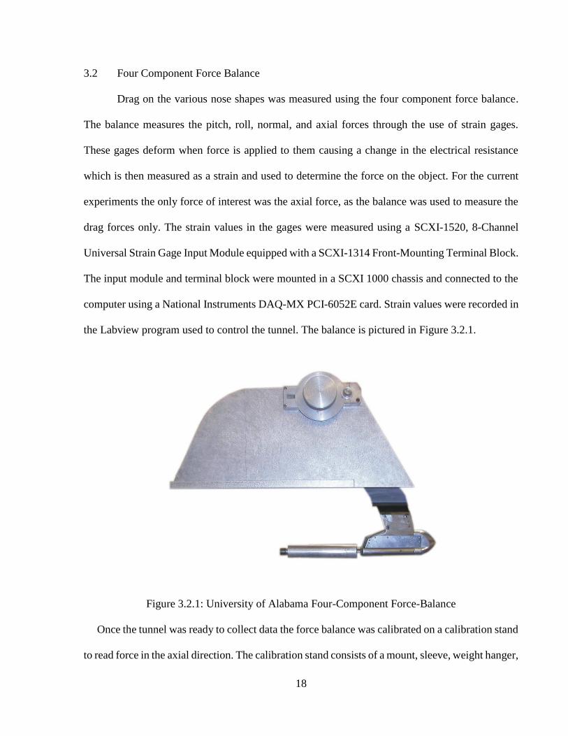
3.2 Four Component Force Balance
Drag on the various nose shapes was measured using the four component force balance.
The balance measures the pitch, roll, normal, and axial forces through the use of strain gages.
These gages deform when force is applied to them causing a change in the electrical resistance
which is then measured as a strain and used to determine the force on the object. For the current
experiments the only force of interest was the axial force, as the balance was used to measure the
drag forces only. The strain values in the gages were measured using a SCXI-1520, 8-Channel
Universal Strain Gage Input Module equipped with a SCXI-1314 Front-Mounting Terminal Block.
The input module and terminal block were mounted in a SCXI 1000 chassis and connected to the
computer using a National Instruments DAQ-MX PCI-6052E card. Strain values were recorded in
the Labview program used to control the tunnel. The balance is pictured in Figure 3.2.1.
Figure 3.2.1: University of Alabama Four-Component Force-Balance
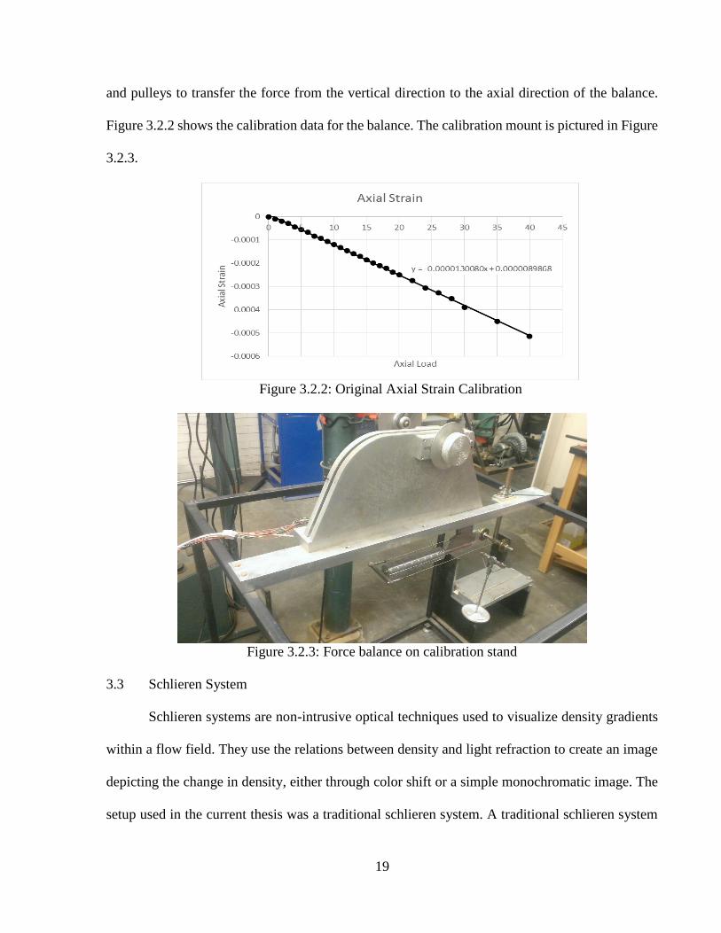
Once the tunnel was ready to collect data the force balance was calibrated on a calibration stand
to read force in the axial direction. The calibration stand consists of a mount, sleeve, weight hanger,
19
and pulleys to transfer the force from the vertical direction to the axial direction of the balance.
Figure 3.2.2 shows the calibration data for the balance. The calibration mount is pictured in Figure
3.2.3.
Figure 3.2.2: Original Axial Strain Calibration
Figure 3.2.3: Force balance on calibration stand
3.3 Schlieren System
Schlieren systems are non-intrusive optical techniques used to visualize density gradients
within a flow field. They use the relations between density and light refraction to create an image
depicting the change in density, either through color shift or a simple monochromatic image. The
setup used in the current thesis was a traditional schlieren system. A traditional schlieren system
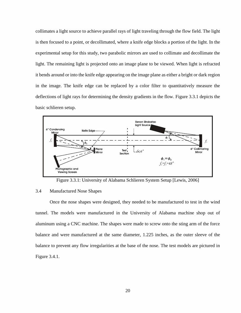
20
collimates a light source to achieve parallel rays of light traveling through the flow field. The light
is then focused to a point, or decollimated, where a knife edge blocks a portion of the light. In the
experimental setup for this study, two parabolic mirrors are used to collimate and decollimate the
light. The remaining light is projected onto an image plane to be viewed. When light is refracted
it bends around or into the knife edge appearing on the image plane as either a bright or dark region
in the image. The knife edge can be replaced by a color filter to quantitatively measure the
deflections of light rays for determining the density gradients in the flow. Figure 3.3.1 depicts the
basic schlieren setup.
Figure 3.3.1: University of Alabama Schlieren System Setup [Lewis, 2006]
3.4 Manufactured Nose Shapes
Once the nose shapes were designed, they needed to be manufactured to test in the wind
tunnel. The models were manufactured in the University of Alabama machine shop out of
aluminum using a CNC machine. The shapes were made to screw onto the sting arm of the force
balance and were manufactured at the same diameter, 1.225 inches, as the outer sleeve of the
balance to prevent any flow irregularities at the base of the nose. The test models are pictured in
Figure 3.4.1.

21
Figure 3.4.1: Models used in Drag Testing
22
CHAPTER 4
RESULTS AND DISCUSSION
In this chapter force balance measurements and the determination of the drag coefficients
are described in detail. Calculated drag coefficient values for different nose shapes are compared
to each other.
4.1 Drag Measurement Method
Measurements with the force-balance measurements require the calibration of the balance
prior to the experiments. The balance calibration is determined by using the calibration stand
described in Chapter 2. The balance was recalibrated any time a modification was made to the
balance.
In the early stages of the experiments the balance was not able to read accurate results.
The balance read erroneous results even though the calibration was very repeatable. A plot of the
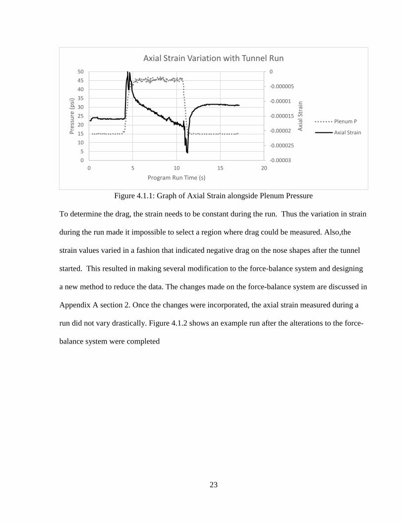
strain readings during a tunnel run at this stage can be found in Figure 4.1.1 The plenum pressure
is also plotted alongside the axial strain to show that the plenum pressure and thus the static
pressure in the test section were kept relatively constant.
23
Figure 4.1.1: Graph of Axial Strain alongside Plenum Pressure
To determine the drag, the strain needs to be constant during the run. Thus the variation in strain
during the run made it impossible to select a region where drag could be measured. Also,the
strain values varied in a fashion that indicated negative drag on the nose shapes after the tunnel
started. This resulted in making several modification to the force-balance system and designing
a new method to reduce the data. The changes made on the force-balance system are discussed in
Appendix A section 2. Once the changes were incorporated, the axial strain measured during a
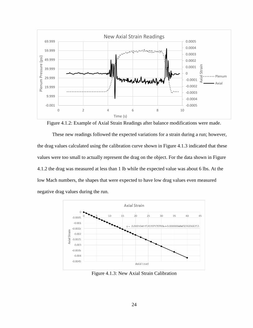
run did not vary drastically. Figure 4.1.2 shows an example run after the alterations to the force-
balance system were completed
-0.00003
-0.000025
-0.00002
-0.000015
-0.00001
-0.000005
0
0
5
10
15
20
25
30
35
40
45
50
0 5 10 15 20
Axi
al S
trai
n
Pre
ssu
re (
psi
)
Program Run Time (s)
Axial Strain Variation with Tunnel Run
Plenum P
Axial Strain
24
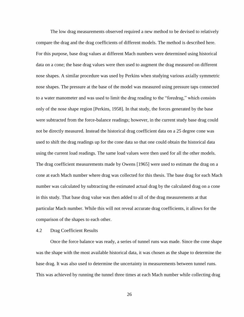
Figure 4.1.2: Example of Axial Strain Readings after balance modifications were made.
These new readings followed the expected variations for a strain during a run; however,
the drag values calculated using the calibration curve shown in Figure 4.1.3 indicated that these
values were too small to actually represent the drag on the object. For the data shown in Figure
4.1.2 the drag was measured at less than 1 lb while the expected value was about 6 lbs. At the
low Mach numbers, the shapes that were expected to have low drag values even measured
negative drag values during the run.
Figure 4.1.3: New Axial Strain Calibration
-0.0005
-0.0004
-0.0003
-0.0002
-0.0001
0
0.0001
0.0002
0.0003
0.0004
0.0005
-0.001
9.999
19.999
29.999
39.999
49.999
59.999
69.999
0 2 4 6 8 10
Axi
al S
trai
n
Ple
nu
m P
ress
ure
(p
si)
Time (s)
New Axial Strain Readings
Plenum
Axial
25
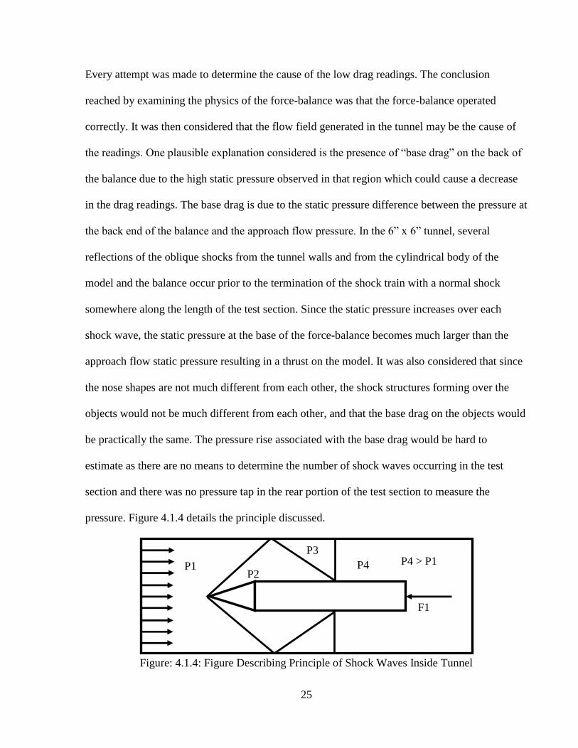
Every attempt was made to determine the cause of the low drag readings. The conclusion
reached by examining the physics of the force-balance was that the force-balance operated
correctly. It was then considered that the flow field generated in the tunnel may be the cause of
the readings. One plausible explanation considered is the presence of “base drag” on the back of
the balance due to the high static pressure observed in that region which could cause a decrease
in the drag readings. The base drag is due to the static pressure difference between the pressure at
the back end of the balance and the approach flow pressure. In the 6” x 6” tunnel, several
reflections of the oblique shocks from the tunnel walls and from the cylindrical body of the
model and the balance occur prior to the termination of the shock train with a normal shock
somewhere along the length of the test section. Since the static pressure increases over each
shock wave, the static pressure at the base of the force-balance becomes much larger than the
approach flow static pressure resulting in a thrust on the model. It was also considered that since
the nose shapes are not much different from each other, the shock structures forming over the
objects would not be much different from each other, and that the base drag on the objects would
be practically the same. The pressure rise associated with the base drag would be hard to
estimate as there are no means to determine the number of shock waves occurring in the test
section and there was no pressure tap in the rear portion of the test section to measure the
pressure. Figure 4.1.4 details the principle discussed.
Figure: 4.1.4: Figure Describing Principle of Shock Waves Inside Tunnel
P1 P2
P3
P4 P4 > P1
F1
26
The low drag measurements observed required a new method to be devised to relatively
compare the drag and the drag coefficients of different models. The method is described here.
For this purpose, base drag values at different Mach numbers were determined using historical
data on a cone; the base drag values were then used to augment the drag measured on different
nose shapes. A similar procedure was used by Perkins when studying various axially symmetric
nose shapes. The pressure at the base of the model was measured using pressure taps connected
to a water manometer and was used to limit the drag reading to the “foredrag,” which consists
only of the nose shape region [Perkins, 1958]. In that study, the forces generated by the base
were subtracted from the force-balance readings; however, in the current study base drag could
not be directly measured. Instead the historical drag coefficient data on a 25 degree cone was
used to shift the drag readings up for the cone data so that one could obtain the historical data
using the current load readings. The same load values were then used for all the other models.
The drag coefficient measurements made by Owens [1965] were used to estimate the drag on a
cone at each Mach number where drag was collected for this thesis. The base drag for each Mach
number was calculated by subtracting the estimated actual drag by the calculated drag on a cone
in this study. That base drag value was then added to all of the drag measurements at that
particular Mach number. While this will not reveal accurate drag coefficients, it allows for the
comparison of the shapes to each other.
4.2 Drag Coefficient Results
Once the force balance was ready, a series of tunnel runs was made. Since the cone shape
was the shape with the most available historical data, it was chosen as the shape to determine the
base drag. It was also used to determine the uncertainty in measurements between tunnel runs.
This was achieved by running the tunnel three times at each Mach number while collecting drag
27
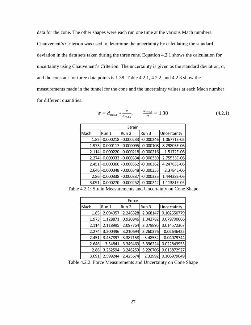
data for the cone. The other shapes were each run one time at the various Mach numbers.
Chauvenent’s Criterion was used to determine the uncertainty by calculating the standard
deviation in the data sets taken during the three runs. Equation 4.2.1 shows the calculation for
uncertainty using Chauvenent’s Criterion. The uncertainty is given as the standard deviation, σ,
and the constant for three data points is 1.38. Table 4.2.1, 4.2.2, and 4.2.3 show the
measurements made in the tunnel for the cone and the uncertainty values at each Mach number
for different quantities.
𝜎 = 𝑑𝑚𝑎𝑥 ∗𝜎
𝑑𝑚𝑎𝑥,
𝑑𝑚𝑎𝑥
𝜎= 1.38 (4.2.1)
Table 4.2.1: Strain Measurements and Uncertainty on Cone Shape
Table 4.2.2: Force Measurements and Uncertainty on Cone Shape
Mach Run 1 Run 2 Run 3 Uncertainty
1.85 -0.000218 -0.000233 -0.000246 1.06771E-05
1.973 -0.000117 -0.000095 -0.000108 8.29805E-06
2.114 -0.000220 -0.000218 -0.000216 1.5172E-06
2.274 -0.000333 -0.000334 -0.000339 2.75533E-06
2.451 -0.000360 -0.000352 -0.000362 4.24763E-06
2.646 -0.000348 -0.000348 -0.000353 2.3784E-06
2.86 -0.000338 -0.000337 -0.000335 1.44438E-06
3.091 -0.000270 -0.000252 -0.000242 1.11381E-05
Strain
Mach Run 1 Run 2 Run 3 Uncertainty
1.85 2.094957 2.246328 2.368147 0.102550779
1.973 1.128871 0.920846 1.042782 0.079700666
2.114 2.118995 2.097764 2.079895 0.014572367
2.274 3.200496 3.210694 3.260376 0.02646425
2.451 3.457897 3.387158 3.48532 0.04079744
2.646 3.34841 3.349463 3.396224 0.022843953
2.86 3.252594 3.246253 3.220706 0.013872927
3.091 2.599244 2.425674 2.32992 0.106979049
Force
28
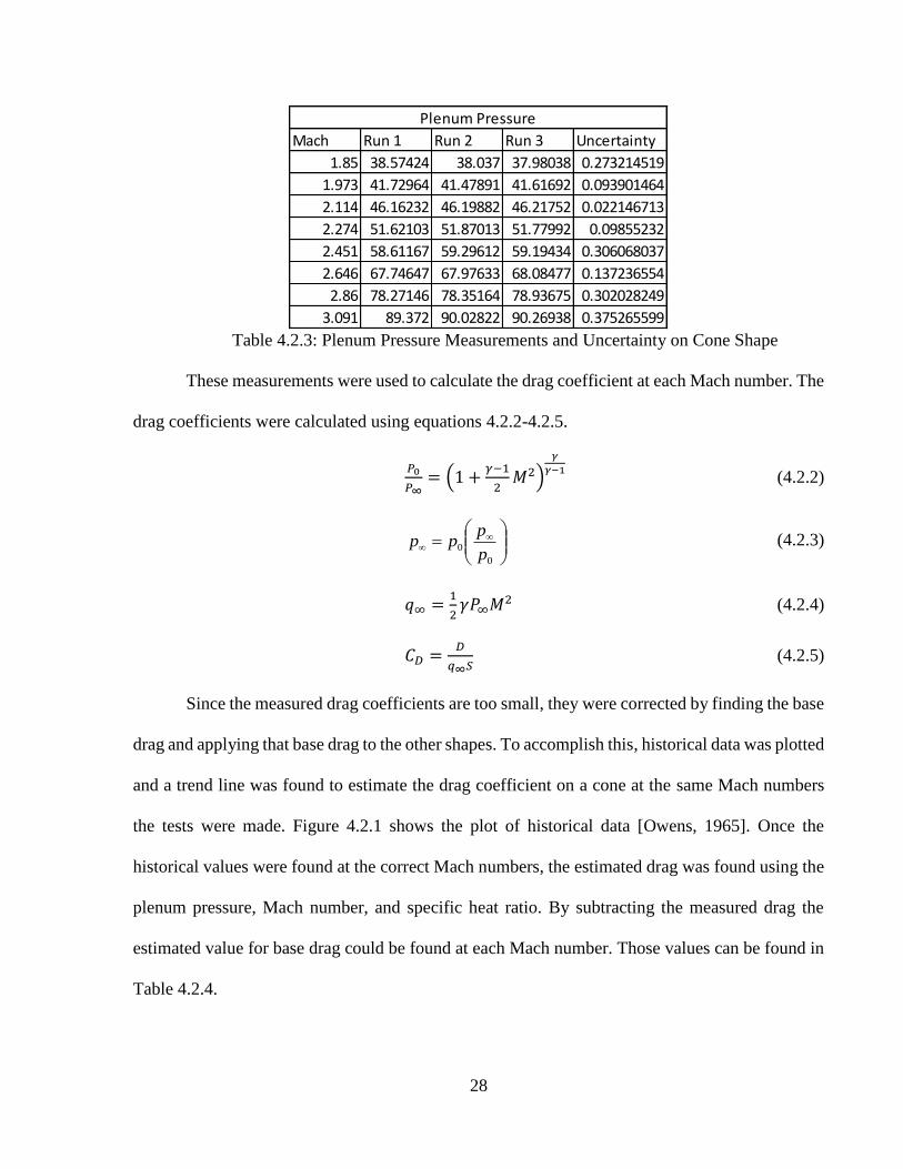
Table 4.2.3: Plenum Pressure Measurements and Uncertainty on Cone Shape
These measurements were used to calculate the drag coefficient at each Mach number. The
drag coefficients were calculated using equations 4.2.2-4.2.5.
𝑃0
𝑃∞= (1 +
𝛾−1
2𝑀2)
𝛾
𝛾−1 (4.2.2)
0
0p
ppp (4.2.3)
𝑞∞ =1
2𝛾𝑃∞𝑀2 (4.2.4)
𝐶𝐷 =𝐷
𝑞∞𝑆 (4.2.5)
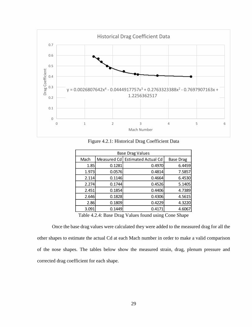
Since the measured drag coefficients are too small, they were corrected by finding the base
drag and applying that base drag to the other shapes. To accomplish this, historical data was plotted
and a trend line was found to estimate the drag coefficient on a cone at the same Mach numbers
the tests were made. Figure 4.2.1 shows the plot of historical data [Owens, 1965]. Once the
historical values were found at the correct Mach numbers, the estimated drag was found using the
plenum pressure, Mach number, and specific heat ratio. By subtracting the measured drag the
estimated value for base drag could be found at each Mach number. Those values can be found in
Table 4.2.4.
Mach Run 1 Run 2 Run 3 Uncertainty
1.85 38.57424 38.037 37.98038 0.273214519
1.973 41.72964 41.47891 41.61692 0.093901464
2.114 46.16232 46.19882 46.21752 0.022146713
2.274 51.62103 51.87013 51.77992 0.09855232
2.451 58.61167 59.29612 59.19434 0.306068037
2.646 67.74647 67.97633 68.08477 0.137236554
2.86 78.27146 78.35164 78.93675 0.302028249
3.091 89.372 90.02822 90.26938 0.375265599
Plenum Pressure
29
Figure 4.2.1: Historical Drag Coefficient Data
Table 4.2.4: Base Drag Values found using Cone Shape
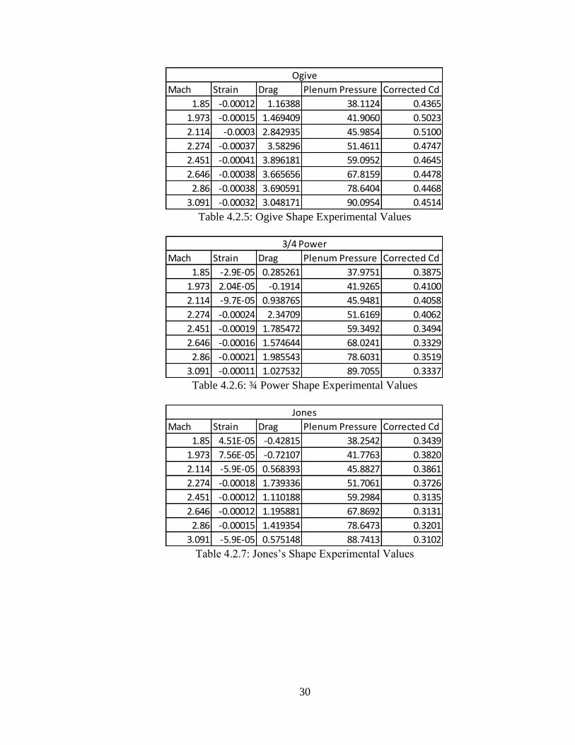
Once the base drag values were calculated they were added to the measured drag for all the
other shapes to estimate the actual Cd at each Mach number in order to make a valid comparison
of the nose shapes. The tables below show the measured strain, drag, plenum pressure and
corrected drag coefficient for each shape.
y = 0.0026807642x4 - 0.0444917757x3 + 0.2763323388x2 - 0.7697907163x + 1.2256362517
0
0.1
0.2
0.3
0.4
0.5
0.6
0.7
0 1 2 3 4 5 6
Dra
g C
oef
fici
ent
Mach Number
Historical Drag Coefficient Data
Mach Measured Cd Estimated Actual Cd Base Drag
1.85 0.1281 0.4970 6.4459
1.973 0.0576 0.4814 7.5857
2.114 0.1146 0.4664 6.4530
2.274 0.1744 0.4526 5.1405
2.451 0.1854 0.4406 4.7389
2.646 0.1828 0.4306 4.5615
2.86 0.1809 0.4229 4.3220
3.091 0.1449 0.4171 4.6067
Base Drag Values
30
Table 4.2.5: Ogive Shape Experimental Values
Table 4.2.6: ¾ Power Shape Experimental Values
Table 4.2.7: Jones’s Shape Experimental Values
Mach Strain Drag Plenum Pressure Corrected Cd
1.85 -0.00012 1.16388 38.1124 0.4365
1.973 -0.00015 1.469409 41.9060 0.5023
2.114 -0.0003 2.842935 45.9854 0.5100
2.274 -0.00037 3.58296 51.4611 0.4747
2.451 -0.00041 3.896181 59.0952 0.4645
2.646 -0.00038 3.665656 67.8159 0.4478
2.86 -0.00038 3.690591 78.6404 0.4468
3.091 -0.00032 3.048171 90.0954 0.4514
Ogive
Mach Strain Drag Plenum Pressure Corrected Cd
1.85 -2.9E-05 0.285261 37.9751 0.3875
1.973 2.04E-05 -0.1914 41.9265 0.4100
2.114 -9.7E-05 0.938765 45.9481 0.4058
2.274 -0.00024 2.34709 51.6169 0.4062
2.451 -0.00019 1.785472 59.3492 0.3494
2.646 -0.00016 1.574644 68.0241 0.3329
2.86 -0.00021 1.985543 78.6031 0.3519
3.091 -0.00011 1.027532 89.7055 0.3337
3/4 Power
Mach Strain Drag Plenum Pressure Corrected Cd
1.85 4.51E-05 -0.42815 38.2542 0.3439
1.973 7.56E-05 -0.72107 41.7763 0.3820
2.114 -5.9E-05 0.568393 45.8827 0.3861
2.274 -0.00018 1.739336 51.7061 0.3726
2.451 -0.00012 1.110188 59.2984 0.3135
2.646 -0.00012 1.195881 67.8692 0.3131
2.86 -0.00015 1.419354 78.6473 0.3201
3.091 -5.9E-05 0.575148 88.7413 0.3102
Jones

31
Table 4.2.8: New Shape Experimental Values
Figure 4.2.2: Corrected Drag Coefficient Values
After calculating the drag coefficient values for each shape, the values were plotted against
the Mach number alongside the historical data for the cone shape. This is shown in Figure 4.2.2.
This will show how the trend compares with the historical data. It was also of interest to plot the
relative values to the cone and those values can be found in Figure 4.2.3.
Mach Strain Drag Plenum Pressure Corrected Cd
1.85 7.68E-05 -0.73262 37.9830 0.3289
1.973 7.52E-05 -0.71733 41.8120 0.3819
2.114 -4.8E-05 0.467603 45.9712 0.3798
2.274 -0.00011 1.103514 50.7528 0.3445
2.451 -9.6E-05 0.926785 59.2073 0.3042
2.646 -8.5E-05 0.819736 67.8803 0.2926
2.86 -0.00012 1.152559 78.5884 0.3054
3.091 -6.6E-05 0.634841 90.0916 0.3091
New
0.275
0.325
0.375
0.425
0.475
0.525
1.85 2.05 2.25 2.45 2.65 2.85 3.05
Dra
g C
oef
fici
ent
Mach Number
Drag Coefficient Values
Cone Ogive 3/4 Power Jones New
32
Figure 4.2.3: Drag Coefficient Values Relative to Cone
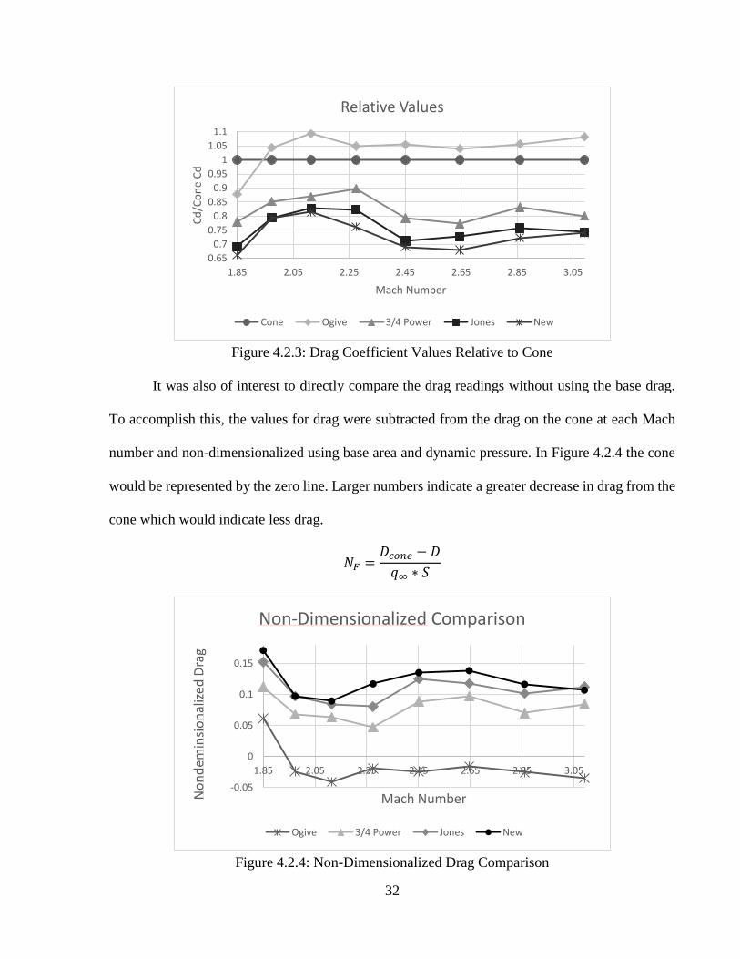
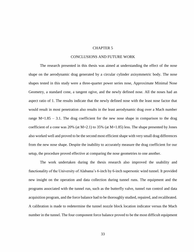
It was also of interest to directly compare the drag readings without using the base drag.
To accomplish this, the values for drag were subtracted from the drag on the cone at each Mach
number and non-dimensionalized using base area and dynamic pressure. In Figure 4.2.4 the cone
would be represented by the zero line. Larger numbers indicate a greater decrease in drag from the
cone which would indicate less drag.
𝑁𝐹 =𝐷𝑐𝑜𝑛𝑒 − 𝐷
𝑞∞ ∗ 𝑆
Figure 4.2.4: Non-Dimensionalized Drag Comparison
0.65
0.7
0.75
0.8
0.85
0.9
0.95
1
1.05
1.1
1.85 2.05 2.25 2.45 2.65 2.85 3.05
Cd
/Co
ne
Cd
Mach Number
Relative Values
Cone Ogive 3/4 Power Jones New
-0.05
0
0.05
0.1
0.15
1.85 2.05 2.25 2.45 2.65 2.85 3.05
No
nd
emin
sio
nal
ized
Dra
g
Mach Number
Non-Dimensionalized Comparison
Ogive 3/4 Power Jones New
33
CHAPTER 5
CONCLUSIONS AND FUTURE WORK
The research presented in this thesis was aimed at understanding the effect of the nose
shape on the aerodynamic drag generated by a circular cylinder axisymmetric body. The nose
shapes tested in this study were a three-quarter power series nose, Approximate Minimal Nose
Geometry, a standard cone, a tangent ogive, and the newly defined nose. All the noses had an
aspect ratio of 1. The results indicate that the newly defined nose with the least nose factor that
would result in most penetration also results in the least aerodynamic drag over a Mach number
range M=1.85 – 3.1. The drag coefficient for the new nose shape in comparison to the drag
coefficient of a cone was 20% (at M=2.1) to 35% (at M=1.85) less. The shape presented by Jones
also worked well and proved to be the second most efficient shape with very small drag differences
from the new nose shape. Despite the inability to accurately measure the drag coefficient for our
setup, the procedure proved effective at comparing the nose geometries to one another.
The work undertaken during the thesis research also improved the usability and
functionality of the University of Alabama’s 6-inch by 6-inch supersonic wind tunnel. It provided
new insight on the operation and data collection during tunnel runs. The equipment and the
programs associated with the tunnel run, such as the butterfly valve, tunnel run control and data
acquisition program, and the force balance had to be thoroughly studied, repaired, and recalibrated.
A calibration is made to redetermine the tunnel nozzle block location indicator versus the Mach
number in the tunnel. The four component force balance proved to be the most difficult equipment

34
to work with and required extensive repairs and trouble shooting. An updated run
procedure is also presented and should provide any operator with the knowledge they need to
operate the tunnel effectively with minimal modifications to the control program or control
equipment.
Future Work:
Further understanding of the effect of the nose shape on the drag of axisymmetric bodies
requires more work to be done. One possible improvement on drag measurements procedures
would be installing more pressure taps in the test section and on the back of the model. These
pressure readings would then provide more information about the base drag and would be useful
especially during small drag readings, such as the ones encountered during this study. It was also
considered that a new force balance could be constructed to minimize the interaction of the air
flowing over the force balance and the strain gages inside the force balance.
The tunnel operation could be improved by making additional changes. One change could
be the addition of a heater to reduce the total temperature drop inside the storage tank during a
tunnel run. This is a complicated procedure but would allow making more intricate testing possible
within both high speed tunnels present in the high-bay area. A more accurate calibration should be
considered to ensure the accuracy of the Mach numbers inside the test section of the large
supersonic tunnel. One final addition could be the installation of a mist separator or a dryer on the
pressure supply for the tunnel’s main valve actuator. Along with an accurate pressure regulator it
would be easier to run the tunnel without worrying about water getting into the actuator.
35
REFERENCES
1. Lewis, D., Calibration and Automation of the university of Alabama 6” x 6” Supersonic
Wind Tunnel and Drag Measurements on Bodies of Revolution. M.S. Thesis, Department
of Aerospace engineering and Mechanics, The University of Alabama, Tuscaloosa, AL,
2006.
2. Poncelet, J. V., Cours de Mecanique Industrielle. Paris, 1829.
3. Hill, R., “Cavitation and Influence of Headshape in Attack of Thick Targets by Non-
Deforming Projectiles”, J. Mech. Phys. Solids, vol. 28, pp: 249-263. 1980.
4. Forrestal, M. J., “Penetration into dry porous rock”, Int, J. Solids Struct. 22, 485, 1985.
5. Forrestal, M. J., “Penetration of Strain Hardening Targets with Rigid Spherical Nose
Rods”, J. Appl. Mech., 58, 7, 1991.
6. Forrestal, M. J., Luk, V. K., 1992, “Penetration into Soil Targets”, Int. J. Impact Eng., 12,
3, 1992.
7. Jones, S. E., Rule, W. K.., Jerome, D. M., Klug, R. T., “on the Optimal Nose Geometry
for a rigid Penetrator,” Computational Mechanics, vol. 22, pp: 413-417. 1998.
8. Eggers, Jr., A.J., Resnikoff, M. M., Dennis, D. H., “Bodies of Revolution Having
Minimum Drag at High Supersonic Airspeeds”, NACA Report 1306, 1957.
9. Yefremov, N. L., Kraiko, A.I., P’yankov, K. S., Takovitskii, S. A., 2006, “The
construction of a nose shape of minimum drag for specified external dimensions and
volume using Euler equations,” Journal of Applied Mathematics and Mechanics 70 912-
923, 2006.
10. Takovitskii, S. A., “The construction of symmetric nose shapes of minimum wave drag”,
Journal of Applied Mathematics and Mechanics 70 373-377, 2006a.
11. Takovitskii, S. A., “Analytical Solution in the Problem of Construction Axisymmetric
Noses with Minimum Wave Drag”. Fluid Dynamics, Vol. 41, No. 2, pp: 308-312.
Translated from Izvestiya Rossiiskoi Academii Nauk, mekhanika Zhidkosti I Gaza, No.
2, pp. 157-162. 2006b.
36
12. Foster N. F., Dulikravich, G. S., “Three-Dimensional Aerodynamic Shape Optimization
Using Genetic and Gradient Search Algorithms”, Journal of Spacecraft and Rockets, Vol.
43, no. 1, pp: 137-146, 1997.
13. Lee, J. W., Min, B. Y., Byun, Y. H., Kin, S. J., “Multipoint Nose Shape Optimization of
Space Launcher Using Response Surface Method,” Journal of Spacecraft and Rockets,
Vol. 45, No. 3, pp: 428-437, 2006.
14. Ragnedda, F., Serra, M., “Optimum Shape of HighSpeed Impactor forConcrete Targets
Using PSOA Heuristic,” Engineering, 2, 257-262, 2010.
15. Deepak, N. R., Ray, T., Boyce, R. R., “Evolutionary Algorithm Shape Optimization of a
Hypersonic Flight Experiment Nose Cone,” Journal of Spacecraft and Rockets, Vol. 45,
No. 3, pp: 428-437, 2008.
16. Forrestal, M. J., Thomas, L., Warren, T. L., “Perforation equations for conical and ogival
nose rigid projectiles into aluminum target plates,” International Journal of Impact
Engineering 36 220-225, 2009.
17. Jones, S. E., Ru;e, W. K., “ On the Optimal Nose Geometry for a rigid penetrator,
Including the Effects of Pressure-Dependent Friction,” Internal Journal of Impact
Engineering 24 403-415, 2000.
18. Anderson, J. D., Fundamentals of Aerodynamics, Fourth Edition, McGraw-Hill, 2007.
19. Nott, C.R., Ölçmen, S.M., Lewis, D.R., and Williams, K., “Supersonic, Variable-Throat,
Blow-Down Wind Tunnel Control Using Genetic Algorithms, Neural Networks, and
Gain Scheduled PID”, Applied Intelligence Vol. 29, No. 1 / August, 2008, pp: 79–89.
20. Perkins, Edward W., Jorgensen, Leland H., Sommer, Simon C., “Investigation of the
Drag of Various Axially Symmetric Nose Shapes of Fineness Ratio 3 for Mach Numbers
from 1.24 to 7.4”, National Advisory Committee for Aeronautics Technical report 1386,
January 1958.
21. Owens, Robert V., “Aerodynamic Characteristics of Spherically Blunted Cones at Mach
Numbers From .5 to 5.0,” NASA TN D-3088, Huntsville, AL, December 1965.

37
APPENDIX A
TUNNEL LAB MODIFICATIONS
A1 Tunnel Maintenance and Repairs
Prior to the research conducted for this thesis, the large supersonic tunnel was not used to
collect data for over two years. This caused a few problems with the operation of the wind tunnel
due to the necessity for highly accurate control of the plenum pressure for proper tunnel operation.
When this research began, the tunnel’s pneumatically actuated valve was not functioning. It would
not open to allow air to enter the plenum chamber. This necessitated a few maintenance procedures
to improve the tunnel operations.
The first procedure involved removing the valve to remove the suspected rust built up in
the valves interior. With the valve removed and cleaned it began to function, but not as well as it
did during the development of the tunnels fuzzy logic, PID control system [Lewis, 2006]. This led
to severe issues with maintaining the control of the plenum pressure. After troubleshooting the
control program and adjusting the gains in the PID controller, it was clear that the valve would
need more work. After working with the tunnel to become familiar with its operation, it was
noticed that when disconnecting the pneumatic actuator for the valve a substantial amount of
moisture would be released from the air connection. The actuator used a separate smaller, low
pressure, air compressor without a dedicated dryer to prevent moisture build up in the tank. This
was a known issue as part of the tunnel run procedure required the tank to be drained of moisture
before running; however, the extended period of inactivity had caused moisture to build up within
the actuator as well. To mitigate this issue, a new step was added to the tunnel run procedure which
38
requires the user to disconnect the pneumatic actuator before leaving for the day, on the
days the tunnel is used. It is also required that the secondary compressor be drained of any
accumulated water before connecting it to the actuator. Once the actuator was drained of all water,
the tunnel began to function well; and the additional changes made to the control program,
discussed in Appendix A3, allowed for even more precise control of the tunnel run conditions.
A2 Force Balance Repairs and Modifications
Another problem arose when attempting to collect data using the decades old force balance.
In the past, minor repairs had been made to the connections within the force balance to broken and
frayed wires. These repairs were functional but required occasional maintenance and recalibration
of the equipment. It was also determined that the drop in static temperature within the tunnel
caused severe changes in strain readings through the course of a tunnel run. A variety of methods
were attempted to correct this inaccuracy. One early attempt involved estimating the static
temperature through the course of the tunnel run using Mach number relations and comparing that
to strain reading to estimate a correction value for the tunnel runs. Another attempt was made by
gluing a thermocouple into the force balance next to the axial strain gages. While this procedure
seemed functional the necessary equipment to read the thermocouple alongside the data from the
strain gages was not available. In order to overcome this obstacle it was determined that the best
solution was to replace the old strain gages with the new ones, and install an additional gage in a
new orientation that would be used for temperature compensation.
The procedure for installing the new gages was simple yet required accurate work in
confined spaces. The new gages were placed in the same orientation as the old ones, but connected
using a full Wheatstone bridge inside the balance. The old gages had individual sets of wires
running out of the balance and connected in a bridge outside of the balance. There is limited space
39
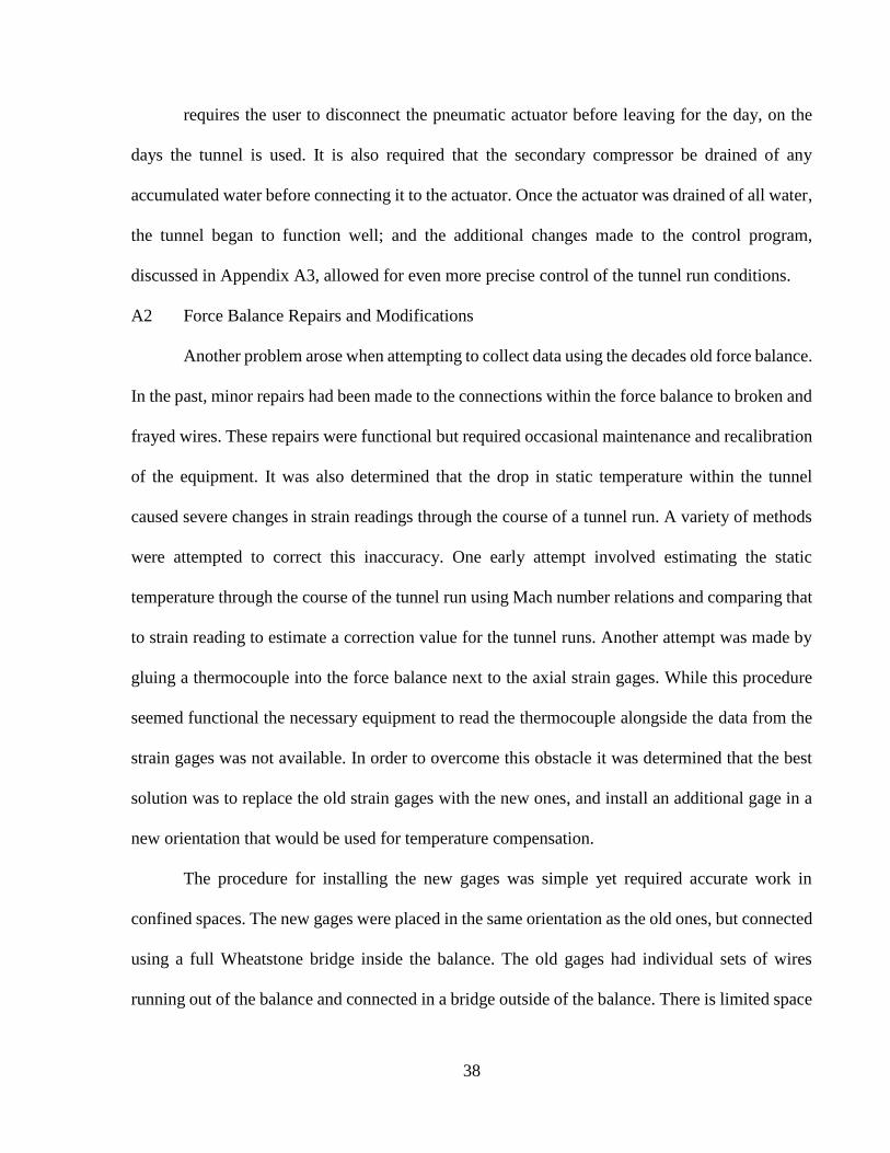
in the conduit sections of the force balance for adding additional wires and the addition of an extra
strain gage necessitated this change. A diagram of the force balance with the highlighted changes
is pictured in Figure A2.1
Figure A2.1: Force Balance Strain Gage Locations and Modifications
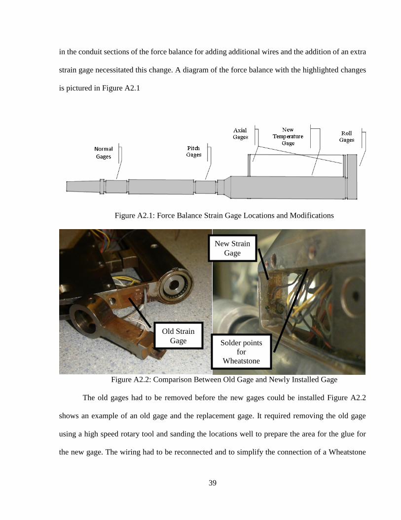
Figure A2.2: Comparison Between Old Gage and Newly Installed Gage
The old gages had to be removed before the new gages could be installed Figure A2.2
shows an example of an old gage and the replacement gage. It required removing the old gage
using a high speed rotary tool and sanding the locations well to prepare the area for the glue for
the new gage. The wiring had to be reconnected and to simplify the connection of a Wheatstone
Old Strain
Gage
New Strain
Gage
Solder points
for
Wheatstone
Bridge
40
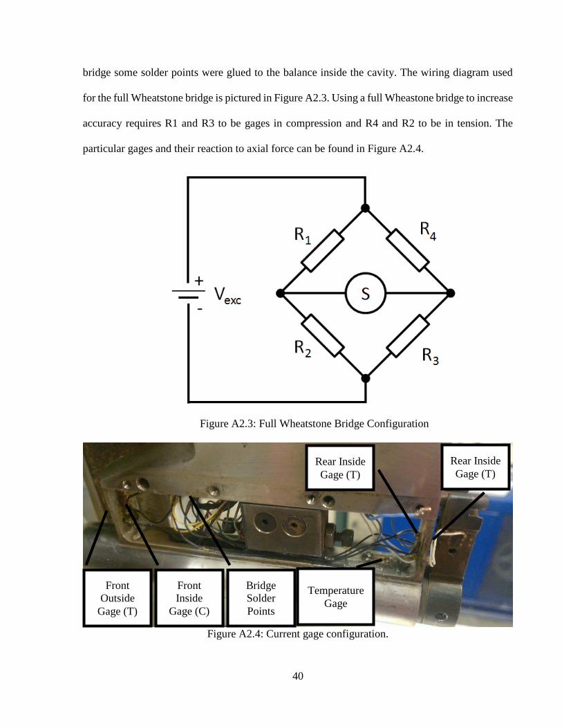
bridge some solder points were glued to the balance inside the cavity. The wiring diagram used
for the full Wheatstone bridge is pictured in Figure A2.3. Using a full Wheastone bridge to increase
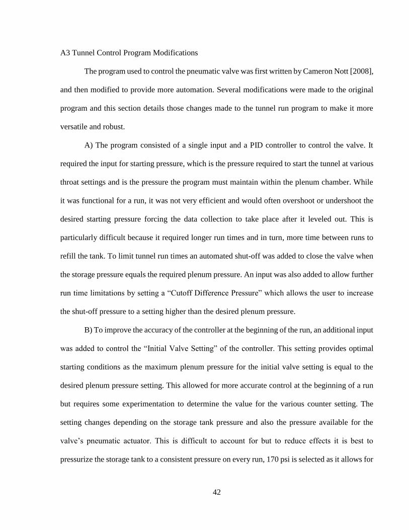
accuracy requires R1 and R3 to be gages in compression and R4 and R2 to be in tension. The
particular gages and their reaction to axial force can be found in Figure A2.4.
Figure A2.3: Full Wheatstone Bridge Configuration
Figure A2.4: Current gage configuration.
Front
Outside
Gage (T)
Front
Inside
Gage (C)
Rear Inside
Gage (T)
Bridge
Solder
Points
Temperature
Gage
Rear Inside
Gage (T)

41
The new gage was placed in a quarter Wheatstone bridge with three 50 ohm resistors which
is also the resistance of the newly installed temperature strain gage. The new gages worked well;
however, temperature compensation proved ineffective for the data processing.
To limit interaction with the temperature, the gage region of the force balance was coated
with a rubber insulation. This produced promising results though the coating peeled off on the rear
of the balance during the first run. To help prevent this, an additional coat of polyurethane was
applied to the rubber insulation to strengthen the insulation. To close any more gaps, a layer of
aluminum tape was also added in regions where it would not restrict the motion of the sting arm
and reduce readings made by the axial gage. Pictures of the insulation can be found in Figure A2.5.
Figure Figure A2.5: Insulation applied to the inside and outside of the force balance.
While the insulation did help reduce temperature interaction it was only effective for the
first couple seconds of the tunnel run. The last attempt at reducing this was to increase the
interaction with axial force. There are two screws located inside the balance that limit the
horizontal motion of the sting arm inside the force balance. Loosening both screws so they do
not limit the sting at all, provided a better axial reading with minimal reaction to other forces or
temperature. This has the downside of reducing the max force that can be safely applied to the
balance; however, the estimated max force applied to these nose shapes was around 10 lbs, and
the balance was tested to 40 lbs during calibration to ensure it would not break during a tunnel
run.
42
A3 Tunnel Control Program Modifications
The program used to control the pneumatic valve was first written by Cameron Nott [2008],
and then modified to provide more automation. Several modifications were made to the original
program and this section details those changes made to the tunnel run program to make it more
versatile and robust.
A) The program consisted of a single input and a PID controller to control the valve. It
required the input for starting pressure, which is the pressure required to start the tunnel at various
throat settings and is the pressure the program must maintain within the plenum chamber. While
it was functional for a run, it was not very efficient and would often overshoot or undershoot the
desired starting pressure forcing the data collection to take place after it leveled out. This is
particularly difficult because it required longer run times and in turn, more time between runs to
refill the tank. To limit tunnel run times an automated shut-off was added to close the valve when
the storage pressure equals the required plenum pressure. An input was also added to allow further
run time limitations by setting a “Cutoff Difference Pressure” which allows the user to increase
the shut-off pressure to a setting higher than the desired plenum pressure.
B) To improve the accuracy of the controller at the beginning of the run, an additional input
was added to control the “Initial Valve Setting” of the controller. This setting provides optimal
starting conditions as the maximum plenum pressure for the initial valve setting is equal to the
desired plenum pressure setting. This allowed for more accurate control at the beginning of a run
but requires some experimentation to determine the value for the various counter setting. The
setting changes depending on the storage tank pressure and also the pressure available for the
valve’s pneumatic actuator. This is difficult to account for but to reduce effects it is best to
pressurize the storage tank to a consistent pressure on every run, 170 psi is selected as it allows for

43
reasonable run times at the highest Mach numbers, and short refill times at the lower speed tunnel
runs. To ensure the same pressure is available for the pneumatic actuator on every run the
secondary compressor is drained until it restarts prior to every run. This ensures the secondary tank
is also filled to its maximum pressure for every run. This new procedure improves upon the
accuracy of the former system with the result of nearly identical tunnel runs at individual Mach
numbers.
C) Prior to this research collecting data in the supersonic tunnel required the use of multiple
programs running simultaneously. When attempting to correct for the temperature differential it
became necessary to plot the strain readings alongside the tank pressures during a run. This wasn’t
feasible with two separate programs as the data could not be lined up with the required accuracy.
To solve this, the strain gage program was incorporated into the program used to control the tunnel.
This allowed data from the tunnel run and the strain gages to be collected at the same time intervals
and allowed for a better understanding of the tunnel run’s effect on the strain gage readings.

44
APPENDIX B
6-INCH X 6-INCH TUNNEL OPERATION
During research for this thesis it was found that previous user guides were inadequate when
attempting to use the high speed wind tunnel. To help future tunnel operators, a new procedure
was developed and is included in this appendix. Images are included to make the process easier as
some of the explanations in previous guides proved difficult to understand.
B1 Filling the Storage Tank
Before use of the Wind Tunnel, the storage tank must be filled. To accomplish this there
are two Ingersoll-Rand Compressors along with an I-R Dehumidifier.
1) Turn on power to the compressors. The switch is found in room 135A directly
behind the large tank. It should be in the down switch position.
Figure B1.1: Wind Tunnel Power Switch
2) Press start on the control panel for both compressors.

45
Figure B1.2: Compressor Control Panel
3) Switch dehumidifier to the dryer on setting.
Figure B1.3: Dehumidifier Control Panel
4) Open the blue outlet valve on the dehumidifier slightly until the rattling noise in
the dryer stops (Turn clockwise to open, counterclockwise to close). This valve needs to be
monitored during the filling process. Watch the digital gages on the compressors for pressure
readings to see whether you need to open or close the valve slightly. It is recommended to
maintain a pressure reading on the compressors of 150 to 160 pounds per square inch (psi) until
the valve is fully open. Pressure readings on the compressors will rise as the tank fills.
5) The tank usually fills to a maximum of about 170 psi. It is best to run at the same
storage pressure every run for optimum consistency. Switch off the compressors, turn off the
46
dryer, and close the valve. Occasionally, the dehumidifier will light up the High Humidity
indicator. If this occurs, turn off and then back on the dehumidifier, close off the fill valve, but
continue running the compressors. Let the dryer run through its cycle a few times. Each cycle
takes about 4 minutes with the automatic settings. Once the High Humidity light goes off, start
filling the tank by opening the valve.
B2 Pre-Run Checks
Once the tank is filled to a desired pressure, there are several factors that can change the
run of the tunnel that need to be checked prior to starting the tunnel run. These are usually
completed as the filling procedure is taking place.
1) Check the Main Valve.
To ensure proper valve operation drain the water from the small compressor used to
operate the main valve. This valve has been very troublesome in the past. To maintain optimum
performance capabilities unplug the air supply from the valve when not in use. This prevents
water from entering the pneumatic valve which prevents it from opening. If this occurs there is a
procedure to purge the valve found in the troubleshooting guide. In addition to draining the
compressor each day before wind tunnel use, draining before each run ensures the same pressure
is supplied to the valve each run. Be sure to reattach the supply to the valve after draining each
run.
2) Check to make sure that the tunnel is shut before connecting the pneumatic
valve’s pressure line and always before running the tunnel.
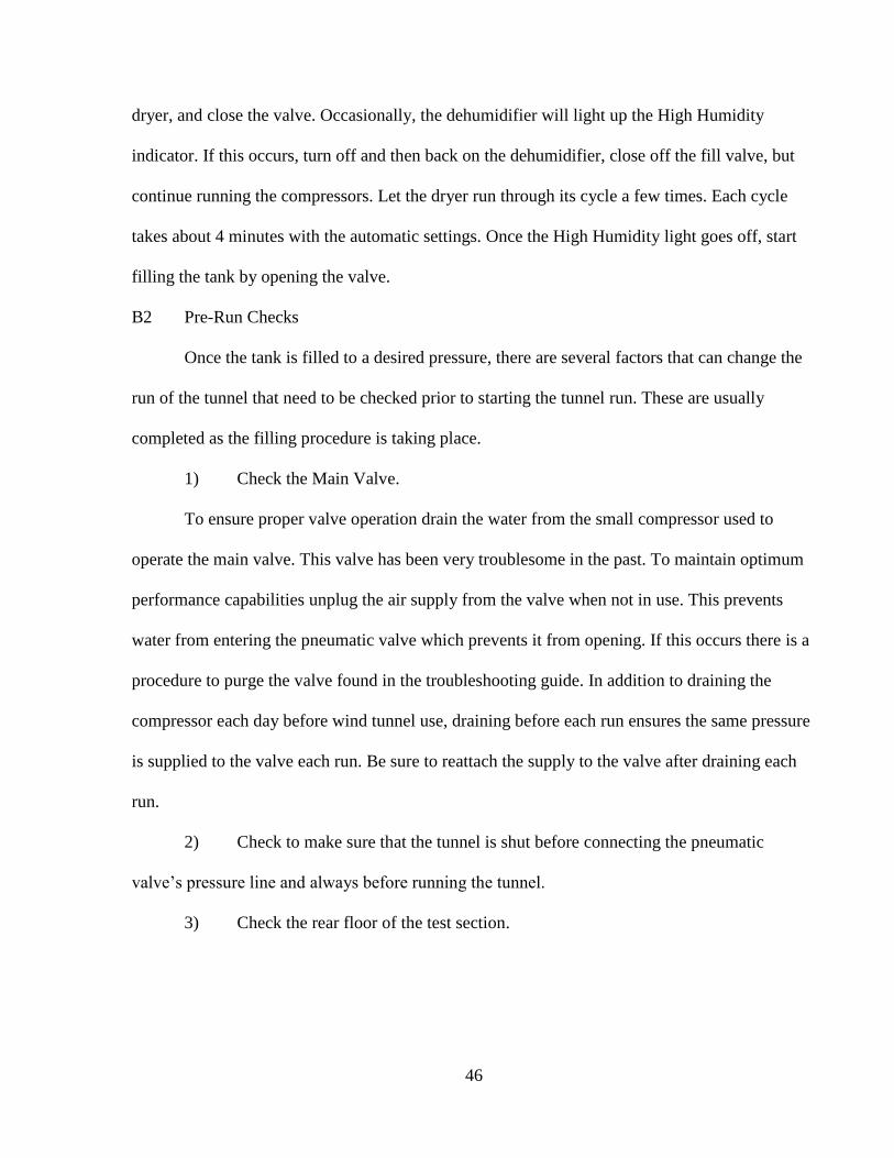
3) Check the rear floor of the test section.

47
Check bottom plate behind the test section. You should unscrew it, slide it forward hard
until it hits the test section floor and then tighten the knob. Pictures of the knob are located in
Figure B2.1.
Figure B2.1: Tunnel region behind the test section and rear plate knob
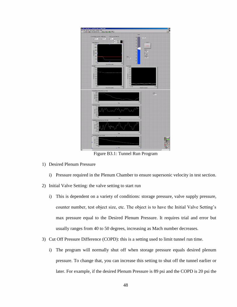
B3 Program for Tunnel Operation
On the control PC, there is a LabView Program called 2014 Controller w 4 comp FB &
temp.vi. It requires certain inputs to run properly. Figure B2.2 shows a screenshot of the
program. The inputs are described below.
48
Figure B3.1: Tunnel Run Program
1) Desired Plenum Pressure
i) Pressure required in the Plenum Chamber to ensure supersonic velocity in test section.
2) Initial Valve Setting: the valve setting to start run
i) This is dependent on a variety of conditions: storage pressure, valve supply pressure,
counter number, test object size, etc. The object is to have the Initial Valve Setting’s
max pressure equal to the Desired Plenum Pressure. It requires trial and error but
usually ranges from 40 to 50 degrees, increasing as Mach number decreases.
3) Cut Off Pressure Difference (COPD): this is a setting used to limit tunnel run time.
i) The program will normally shut off when storage pressure equals desired plenum
pressure. To change that, you can increase this setting to shut off the tunnel earlier or
later. For example, if the desired Plenum Pressure is 89 psi and the COPD is 20 psi the

49
valve will close when storage pressure reaches 109 psi. This decreases the time required
to refill the tank after each run. It is recommended to have the Cut-Off Pressure
Difference set so that the program will stop running when the pressure is 110 psi.
Once the inputs are entered, put on ear protection and sound the alarm, then the start button
on the LabView program can be pressed. The program will pre-load the actuator with air then open
the valve after three seconds. If undershoot or overshoot occurs press the large stop button and
adjust the initial valve setting. Never use LabView’s built in stop button; this will not close the
valve. If the tunnel runs smoothly the Stop button can be pressed and data can be saved.
B4 Troubleshooting
A troubleshooting guide has been made to assist with common problems. It is found in
Table B4.1.
Issue Possible Causes Fixes
Pneumatic valve won’t open Water is in the valve
Computer or control modules
aren’t functioning properly
Compressor for valve isn’t on
or is broken
Drain the water using the
procedure detailed below
Be sure all devices are
plugged in and restart all
systems. Shut off computer
first then unplug all control
devices for a few minutes then
plug everything in and restart
the computer.
Check blue compressor for air
pressure
Compressors will not turn
on
Main power switch is off or at
the wrong setting
Broken compressor
Check that the main power
switch is switched down
Call number on compressor
for help
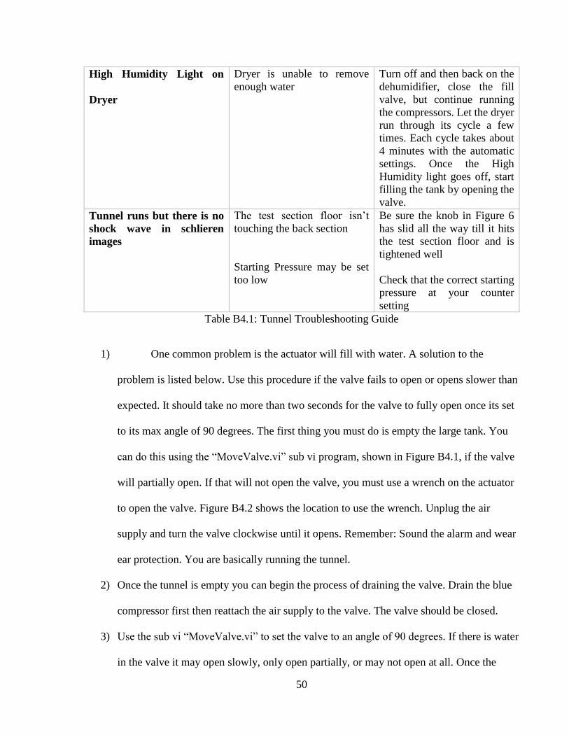
50
High Humidity Light on
Dryer
Dryer is unable to remove
enough water
Turn off and then back on the
dehumidifier, close the fill
valve, but continue running
the compressors. Let the dryer
run through its cycle a few
times. Each cycle takes about
4 minutes with the automatic
settings. Once the High
Humidity light goes off, start
filling the tank by opening the
valve.
Tunnel runs but there is no
shock wave in schlieren
images
The test section floor isn’t
touching the back section
Starting Pressure may be set
too low
Be sure the knob in Figure 6
has slid all the way till it hits
the test section floor and is
tightened well
Check that the correct starting
pressure at your counter
setting
Table B4.1: Tunnel Troubleshooting Guide
1) One common problem is the actuator will fill with water. A solution to the
problem is listed below. Use this procedure if the valve fails to open or opens slower than
expected. It should take no more than two seconds for the valve to fully open once its set
to its max angle of 90 degrees. The first thing you must do is empty the large tank. You
can do this using the “MoveValve.vi” sub vi program, shown in Figure B4.1, if the valve
will partially open. If that will not open the valve, you must use a wrench on the actuator
to open the valve. Figure B4.2 shows the location to use the wrench. Unplug the air
supply and turn the valve clockwise until it opens. Remember: Sound the alarm and wear
ear protection. You are basically running the tunnel.
2) Once the tunnel is empty you can begin the process of draining the valve. Drain the blue
compressor first then reattach the air supply to the valve. The valve should be closed.
3) Use the sub vi “MoveValve.vi” to set the valve to an angle of 90 degrees. If there is water
in the valve it may open slowly, only open partially, or may not open at all. Once the
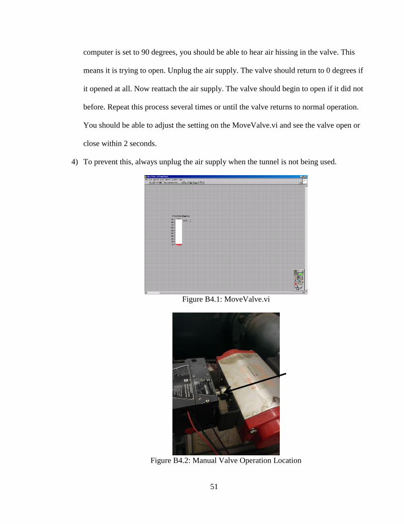
51
computer is set to 90 degrees, you should be able to hear air hissing in the valve. This
means it is trying to open. Unplug the air supply. The valve should return to 0 degrees if
it opened at all. Now reattach the air supply. The valve should begin to open if it did not
before. Repeat this process several times or until the valve returns to normal operation.
You should be able to adjust the setting on the MoveValve.vi and see the valve open or
close within 2 seconds.
4) To prevent this, always unplug the air supply when the tunnel is not being used.
Figure B4.1: MoveValve.vi
Figure B4.2: Manual Valve Operation Location

52
B5 Conclusion
This guide was developed to help future users operate the tunnel with a lesser learning
curve. Many of the procedures outlined required trial and error to learn. It is expected that this
guide will allow smoother tunnel operation so more time can be spent on preforming research in
the tunnel. It is expected that changes to the tunnel will be made over time and hopefully this guide
will be updated as more operators use the tunnel.
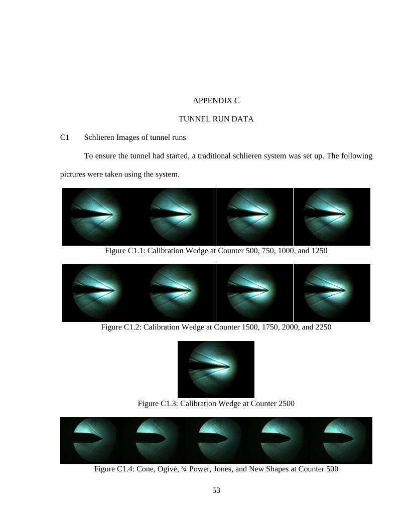
53
APPENDIX C
TUNNEL RUN DATA
C1 Schlieren Images of tunnel runs
To ensure the tunnel had started, a traditional schlieren system was set up. The following
pictures were taken using the system.
Figure C1.1: Calibration Wedge at Counter 500, 750, 1000, and 1250
Figure C1.2: Calibration Wedge at Counter 1500, 1750, 2000, and 2250
Figure C1.3: Calibration Wedge at Counter 2500
Figure C1.4: Cone, Ogive, ¾ Power, Jones, and New Shapes at Counter 500

54
Figure C1.4: Cone, Ogive, ¾ Power, Jones, and New Shapes at Counter 750
Figure C1.5: Cone, Ogive, ¾ Power, Jones, and New Shapes at Counter 1000
Figure C1.6: Cone, Ogive, ¾ Power, Jones, and New Shapes at Counter 1250
Figure C1.7: Cone, Ogive, ¾ Power, Jones, and New Shapes at Counter 1500
Figure C1.8: Cone, Ogive, ¾ Power, Jones, and New Shapes at Counter 1750
Figure C1.9: Cone, Ogive, ¾ Power, Jones, and New Shapes at Counter 2000

55
Figure C1.10: Cone, Ogive, ¾ Power, Jones, and New Shapes at Counter 2250
C2 Tunnel Run Data
Pictured below are plots of the tunnel runs that show the axial strain and the plenum
pressure. The data was collected when both the axial strain and plenum pressure had settled to
reasonably level readings.
Figure C2.1: Cone Run 1 at Counter 500
Figure C2.2: Cone Run 2 at Counter 500
-0.0012
-0.001
-0.0008
-0.0006
-0.0004
-0.0002
0
0.0002
-0.001
4.999
9.999
14.999
19.999
24.999
29.999
34.999
39.999
44.999
0 2 4 6 8 10
Axi
al S
trai
n
Ple
nu
m P
ress
ure
(p
si)
Time (s)
Cone 1 500
Plenum
Axial
-0.0012
-0.001
-0.0008
-0.0006
-0.0004
-0.0002
0
0.0002
-0.001
4.999
9.999
14.999
19.999
24.999
29.999
34.999
39.999
44.999
0 2 4 6 8 10
Axi
al S
trai
n
Ple
nu
m P
ress
ure
Time (s)
Cone 2 500
Plenum
Axial
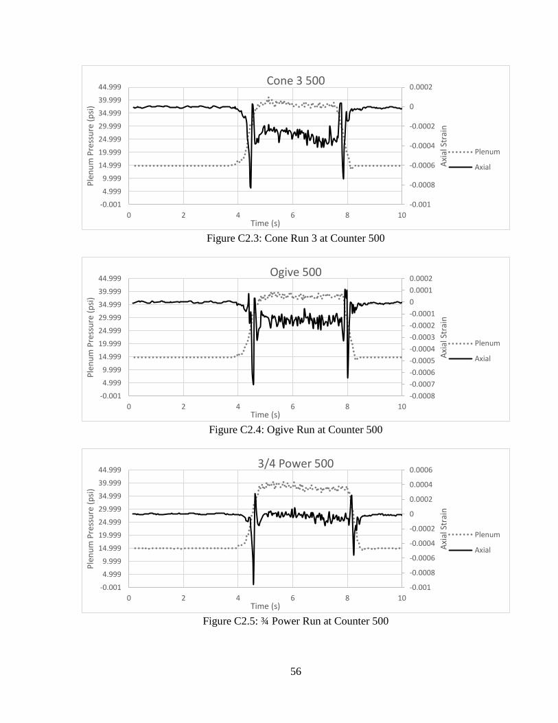
56
Figure C2.3: Cone Run 3 at Counter 500
Figure C2.4: Ogive Run at Counter 500
Figure C2.5: ¾ Power Run at Counter 500
-0.001
-0.0008
-0.0006
-0.0004
-0.0002
0
0.0002
-0.001
4.999
9.999
14.999
19.999
24.999
29.999
34.999
39.999
44.999
0 2 4 6 8 10
Axi
al S
trai
n
Ple
nu
m P
ress
ure
(p
si)
Time (s)
Cone 3 500
Plenum
Axial
-0.0008
-0.0007
-0.0006
-0.0005
-0.0004
-0.0003
-0.0002
-0.0001
0
0.0001
0.0002
-0.001
4.999
9.999
14.999
19.999
24.999
29.999
34.999
39.999
44.999
0 2 4 6 8 10
Axi
al S
trai
n
Ple
nu
m P
ress
ure
(p
si)
Time (s)
Ogive 500
Plenum
Axial
-0.001
-0.0008
-0.0006
-0.0004
-0.0002
0
0.0002
0.0004
0.0006
-0.001
4.999
9.999
14.999
19.999
24.999
29.999
34.999
39.999
44.999
0 2 4 6 8 10
Axi
al S
trai
n
Ple
nu
m P
ress
ure
(p
si)
Time (s)
3/4 Power 500
Plenum
Axial
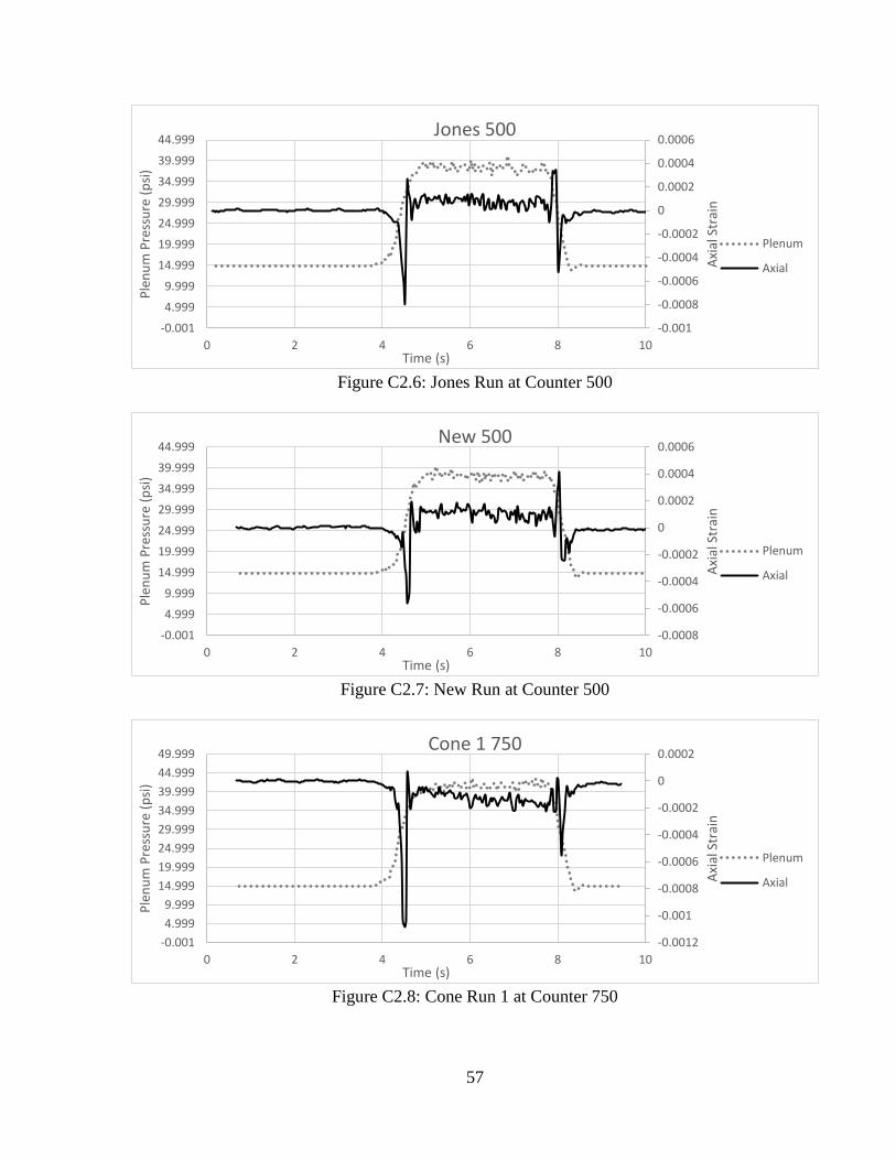
57
Figure C2.6: Jones Run at Counter 500
Figure C2.7: New Run at Counter 500
Figure C2.8: Cone Run 1 at Counter 750
-0.001
-0.0008
-0.0006
-0.0004
-0.0002
0
0.0002
0.0004
0.0006
-0.001
4.999
9.999
14.999
19.999
24.999
29.999
34.999
39.999
44.999
0 2 4 6 8 10
Axi
al S
trai
n
Ple
nu
m P
ress
ure
(p
si)
Time (s)
Jones 500
Plenum
Axial
-0.0008
-0.0006
-0.0004
-0.0002
0
0.0002
0.0004
0.0006
-0.001
4.999
9.999
14.999
19.999
24.999
29.999
34.999
39.999
44.999
0 2 4 6 8 10
Axi
al S
trai
n
Ple
nu
m P
ress
ure
(p
si)
Time (s)
New 500
Plenum
Axial
-0.0012
-0.001
-0.0008
-0.0006
-0.0004
-0.0002
0
0.0002
-0.001
4.999
9.999
14.999
19.999
24.999
29.999
34.999
39.999
44.999
49.999
0 2 4 6 8 10
Axi
al S
trai
n
Ple
nu
m P
ress
ure
(p
si)
Time (s)
Cone 1 750
Plenum
Axial
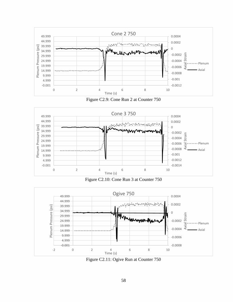
58
Figure C2.9: Cone Run 2 at Counter 750
Figure C2.10: Cone Run 3 at Counter 750
Figure C2.11: Ogive Run at Counter 750
-0.0012
-0.001
-0.0008
-0.0006
-0.0004
-0.0002
0
0.0002
0.0004
-0.001
4.999
9.999
14.999
19.999
24.999
29.999
34.999
39.999
44.999
49.999
0 2 4 6 8 10
Axi
al S
trai
n
Ple
nu
m P
ress
ure
(p
si)
Time (s)
Cone 2 750
Plenum
Axial
-0.0014
-0.0012
-0.001
-0.0008
-0.0006
-0.0004
-0.0002
0
0.0002
0.0004
-0.001
4.999
9.999
14.999
19.999
24.999
29.999
34.999
39.999
44.999
49.999
0 2 4 6 8 10
Axi
al S
trai
n
Ple
nu
m P
ress
ure
(p
si)
Time (s)
Cone 3 750
Plenum
Axial
-0.0008
-0.0006
-0.0004
-0.0002
0
0.0002
0.0004
-0.001
4.999
9.999
14.999
19.999
24.999
29.999
34.999
39.999
44.999
49.999
-2 0 2 4 6 8 10
Axi
al S
trai
n
Ple
nu
m P
ress
ure
(p
si)
Time (s)
Ogive 750
Plenum
Axial

59
Figure C2.12: ¾ Power Run at Counter 750
Figure C2.13: Jones Run at Counter 750
Figure C2.14: New Run at Counter 750
-0.0008
-0.0006
-0.0004
-0.0002
0
0.0002
0.0004
0.0006
-0.001
4.999
9.999
14.999
19.999
24.999
29.999
34.999
39.999
44.999
49.999
-2 0 2 4 6 8 10
Axi
al S
trai
n
Ple
nu
m P
ress
ure
(p
si)
Time (s)
3/4 Power 750
Plenum
Axial
-0.0008
-0.0006
-0.0004
-0.0002
0
0.0002
0.0004
0.0006
-0.001
4.999
9.999
14.999
19.999
24.999
29.999
34.999
39.999
44.999
49.999
-2 0 2 4 6 8 10
Axi
al S
trai
n
Ple
nu
m P
ress
ure
(p
si)
Time (s)
Jones 750
Plenum
Axial
-0.0012
-0.001
-0.0008
-0.0006
-0.0004
-0.0002
0
0.0002
0.0004
0.0006
-0.001
4.999
9.999
14.999
19.999
24.999
29.999
34.999
39.999
44.999
49.999
-2 0 2 4 6 8 10
Axi
al S
trai
n
Ple
nu
m P
ress
ure
(p
si)
Time (s)
New 750
Plenum
Axial

60
Figure C2.15: Cone Run 1 at Counter 1000
Figure C.16: Cone Run 2 at Counter 1000
Figure C.17: Cone Run 3 at Counter 1000
-0.0016
-0.0014
-0.0012
-0.001
-0.0008
-0.0006
-0.0004
-0.0002
0
0.0002
0.0004
-0.001
9.999
19.999
29.999
39.999
49.999
59.999
0 2 4 6 8 10
Axi
al S
trai
n
Ple
nu
m P
ress
ure
(p
si)
Time (s)
Cone 1 1000
Plenum
Axial
-0.0016
-0.0014
-0.0012
-0.001
-0.0008
-0.0006
-0.0004
-0.0002
0
0.0002
-0.001
9.999
19.999
29.999
39.999
49.999
59.999
0 2 4 6 8 10
Axi
al S
trai
n
Ple
nu
m P
ress
ure
(p
si)
Time (s)
Cone 2 1000
Plenum
Axial
-0.0014
-0.0012
-0.001
-0.0008
-0.0006
-0.0004
-0.0002
0
0.0002
0.0004
-0.001
9.999
19.999
29.999
39.999
49.999
59.999
0 2 4 6 8 10
Axi
al S
trai
n
Ple
nu
m P
ress
ure
(p
si)
Time (s)
Cone 3 1000
Plenum
Axial

61
Figure C2.18: Ogive Run at Counter 1000
Figure C2.19: ¾ Power Run at Counter 1000
Figure C2.20: Jones Run at Counter 1000
-0.0012
-0.001
-0.0008
-0.0006
-0.0004
-0.0002
0
0.0002
0.0004
-0.001
9.999
19.999
29.999
39.999
49.999
59.999
-2 0 2 4 6 8 10
Axi
al S
trai
n
Ple
nu
m P
ress
ure
(p
si)
Time (s)
Ogive 1000
Plenum
Axial
-0.0012
-0.001
-0.0008
-0.0006
-0.0004
-0.0002
0
0.0002
0.0004
-0.001
9.999
19.999
29.999
39.999
49.999
59.999
-2 0 2 4 6 8 10
Axi
al S
trai
n
Ple
nu
m P
ress
ure
(p
si)
Time (s)
3/4 Power 1000
Plenum
Axial
-0.0014
-0.0012
-0.001
-0.0008
-0.0006
-0.0004
-0.0002
0
0.0002
0.0004
0.0006
-0.001
4.999
9.999
14.999
19.999
24.999
29.999
34.999
39.999
44.999
49.999
-2 0 2 4 6 8 10
Axi
al S
trai
n
Ple
nu
m P
ress
ure
(p
si)
Time (s)
Jones 1000
Plenum
Axial

62
Figure C2.21: New Run at Counter 1000
Figure C2.22: Cone Run 1 at Counter 1250
Figure C2.23: Cone Run 2 at Counter 1250
-0.0014
-0.0012
-0.001
-0.0008
-0.0006
-0.0004
-0.0002
0
0.0002
0.0004
0.0006
-0.001
4.999
9.999
14.999
19.999
24.999
29.999
34.999
39.999
44.999
49.999
-2 0 2 4 6 8 10
Axi
al S
trai
n
Ple
nu
m P
ress
ure
(p
si)
Time (s)
New 1000
Plenum
Axial
-0.0018
-0.0016
-0.0014
-0.0012
-0.001
-0.0008
-0.0006
-0.0004
-0.0002
0
0.0002
0.0004
-0.001
9.999
19.999
29.999
39.999
49.999
59.999
0 2 4 6 8 10
Axi
al S
trai
n
Ple
nu
m P
ress
ure
(p
si)
Time (s)
Cone 1 1250
Plenum
Axial
-0.001
-0.0008
-0.0006
-0.0004
-0.0002
0
0.0002
0.0004
-0.001
9.999
19.999
29.999
39.999
49.999
59.999
0 2 4 6 8 10
Axi
al S
trai
n
Ple
nu
m P
ress
ure
(p
si)
Time (s)
Cone 2 1250
Plenum
Axial
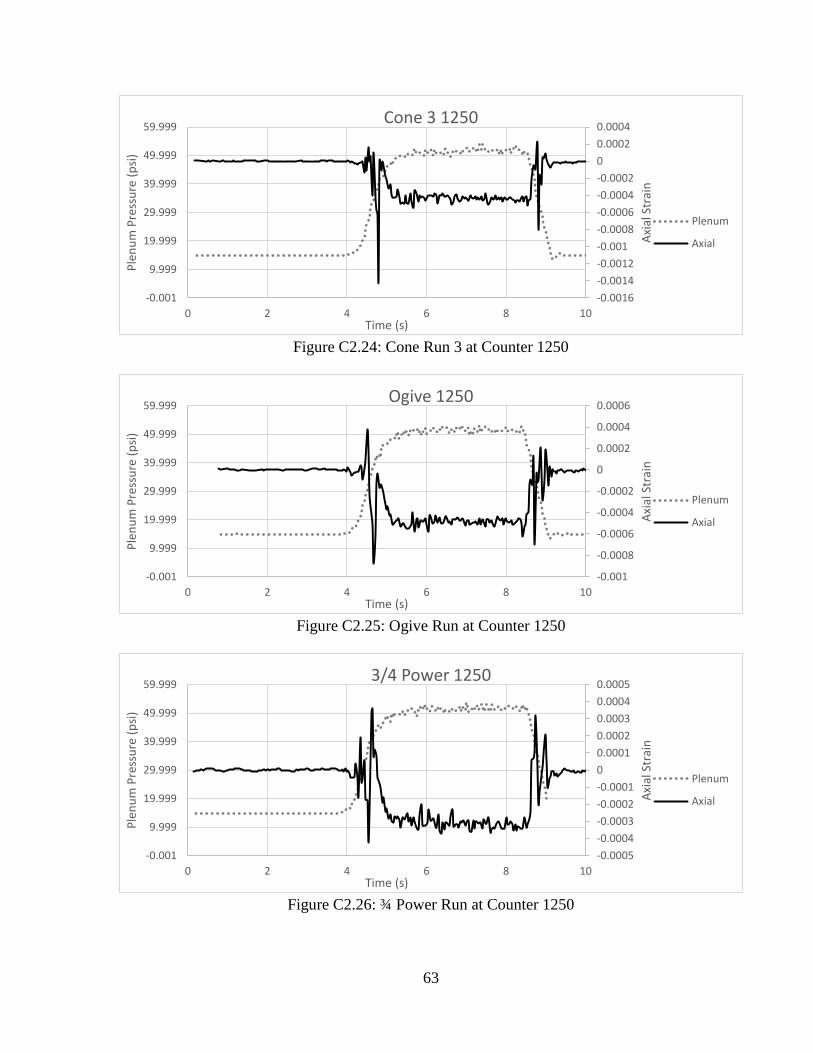
63
Figure C2.24: Cone Run 3 at Counter 1250
Figure C2.25: Ogive Run at Counter 1250
Figure C2.26: ¾ Power Run at Counter 1250
-0.0016
-0.0014
-0.0012
-0.001
-0.0008
-0.0006
-0.0004
-0.0002
0
0.0002
0.0004
-0.001
9.999
19.999
29.999
39.999
49.999
59.999
0 2 4 6 8 10
Axi
al S
trai
n
Ple
nu
m P
ress
ure
(p
si)
Time (s)
Cone 3 1250
Plenum
Axial
-0.001
-0.0008
-0.0006
-0.0004
-0.0002
0
0.0002
0.0004
0.0006
-0.001
9.999
19.999
29.999
39.999
49.999
59.999
0 2 4 6 8 10
Axi
al S
trai
n
Ple
nu
m P
ress
ure
(p
si)
Time (s)
Ogive 1250
Plenum
Axial
-0.0005
-0.0004
-0.0003
-0.0002
-0.0001
0
0.0001
0.0002
0.0003
0.0004
0.0005
-0.001
9.999
19.999
29.999
39.999
49.999
59.999
0 2 4 6 8 10
Axi
al S
trai
n
Ple
nu
m P
ress
ure
(p
si)
Time (s)
3/4 Power 1250
Plenum
Axial

64
Figure C2.27: Jones Run at Counter 1250
Figure C2.28: New Run at Counter 1250
Figure C2.29: Cone Run 1 at Counter 1500
-0.0012
-0.001
-0.0008
-0.0006
-0.0004
-0.0002
0
0.0002
0.0004
0.0006
-0.001
9.999
19.999
29.999
39.999
49.999
59.999
0 2 4 6 8 10
Axi
al S
trai
n
Ple
nu
m P
ress
ure
(p
si)
Time (s)
Jones 1250
Plenum
Axial
-0.001
-0.0008
-0.0006
-0.0004
-0.0002
0
0.0002
0.0004
0.0006
-0.001
9.999
19.999
29.999
39.999
49.999
59.999
0 2 4 6 8 10
Axi
al S
trai
n
Ple
nu
m P
ress
ure
(p
si)
Time (s)
New 1250
Plenum
Axial
-0.001
-0.0008
-0.0006
-0.0004
-0.0002
0
0.0002
0.0004
0.0006
-0.001
9.999
19.999
29.999
39.999
49.999
59.999
69.999
0 2 4 6 8 10
Axi
al S
trai
n
Ple
nu
m P
ress
ure
(p
si)
Time (s)
Cone 1 1500
Plenum
Axial
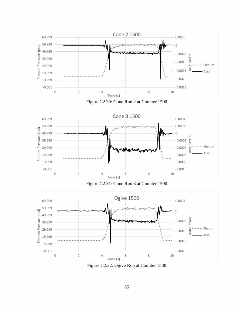
65
Figure C2.30: Cone Run 2 at Counter 1500
Figure C2.31: Cone Run 3 at Counter 1500
Figure C2.32: Ogive Run at Counter 1500
-0.0025
-0.002
-0.0015
-0.001
-0.0005
0
0.0005
-0.001
9.999
19.999
29.999
39.999
49.999
59.999
69.999
0 2 4 6 8 10
Axi
al S
trai
n
Ple
nu
m P
ress
ure
(p
si)
Time (s)
Cone 2 1500
Plenum
Axial
-0.001
-0.0008
-0.0006
-0.0004
-0.0002
0
0.0002
0.0004
-0.001
9.999
19.999
29.999
39.999
49.999
59.999
69.999
0 2 4 6 8 10
Axi
al S
trai
n
Ple
nu
m P
ress
ure
(p
si)
Time (s)
Cone 3 1500
Plenum
Axial
-0.002
-0.0015
-0.001
-0.0005
0
0.0005
-0.001
9.999
19.999
29.999
39.999
49.999
59.999
69.999
0 2 4 6 8 10
Axi
al S
trai
n
Ple
nu
m P
ress
ure
(p
si)
Time (s)
Ogive 1500
Plenum
Axial

66
Figure C2.33: ¾ Power Run at Counter 1500
Figure C2.34: Jones Run at Counter 1500
Figure C2.35: New Run at Counter 1500
-0.0008
-0.0006
-0.0004
-0.0002
0
0.0002
0.0004
0.0006
-0.001
9.999
19.999
29.999
39.999
49.999
59.999
69.999
0 2 4 6 8 10
Axi
al S
trai
n
Ple
nu
m P
ress
ure
(p
si)
Time (s)
3/4 Power 1500
Plenum
Axial
-0.0008
-0.0006
-0.0004
-0.0002
0
0.0002
0.0004
-0.001
9.999
19.999
29.999
39.999
49.999
59.999
69.999
0 2 4 6 8 10
Axi
al S
trai
n
Ple
nu
m P
ress
ure
(p
si)
Time (s)
Jones 1500
Plenum
Axial
-0.0005
-0.0004
-0.0003
-0.0002
-0.0001
0
0.0001
0.0002
0.0003
0.0004
0.0005
-0.001
9.999
19.999
29.999
39.999
49.999
59.999
69.999
0 2 4 6 8 10
Axi
al S
trai
n
Ple
nu
m P
ress
ure
(p
si)
Time (s)
New 1500
Plenum
Axial

67
Figure C2.36: Cone Run 1 at Counter 1750
Figure C2.37: Cone Run 2 at Counter 1750
Figure C2.38: Cone Run 3 at Counter 1750
-0.0012
-0.001
-0.0008
-0.0006
-0.0004
-0.0002
0
0.0002
0.0004
0.0006
-0.001
9.999
19.999
29.999
39.999
49.999
59.999
69.999
79.999
0 2 4 6 8 10
Axi
al S
trai
n
Ple
nu
m P
ress
ure
(p
si)
Time (s)
Cone 1 1750
Plenum
Axial
-0.0014
-0.0012
-0.001
-0.0008
-0.0006
-0.0004
-0.0002
0
0.0002
0.0004
0.0006
-0.001
9.999
19.999
29.999
39.999
49.999
59.999
69.999
79.999
0 2 4 6 8 10
Axi
al S
trai
n
Ple
nu
m P
ress
ure
(p
si)
Time (s)
Cone 2 1750
Plenum
Axial
-0.0012
-0.001
-0.0008
-0.0006
-0.0004
-0.0002
0
0.0002
0.0004
0.0006
-0.001
9.999
19.999
29.999
39.999
49.999
59.999
69.999
79.999
0 2 4 6 8 10
Axi
al S
trai
n
Ple
nu
m P
ress
ure
(p
si)
Time (s)
Cone 3 1750
Plenum
Axial
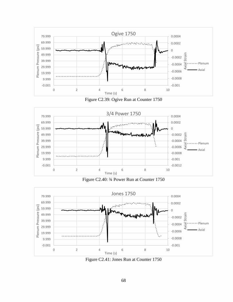
68
Figure C2.39: Ogive Run at Counter 1750
Figure C2.40: ¾ Power Run at Counter 1750
Figure C2.41: Jones Run at Counter 1750
-0.001
-0.0008
-0.0006
-0.0004
-0.0002
0
0.0002
0.0004
-0.001
9.999
19.999
29.999
39.999
49.999
59.999
69.999
79.999
0 2 4 6 8 10
Axi
al S
trai
n
Ple
nu
m P
ress
ure
(p
si)
Time (s)
Ogive 1750
Plenum
Axial
-0.0012
-0.001
-0.0008
-0.0006
-0.0004
-0.0002
0
0.0002
0.0004
-0.001
9.999
19.999
29.999
39.999
49.999
59.999
69.999
79.999
0 2 4 6 8 10
Axi
al S
trai
n
Ple
nu
m P
ress
ure
(p
si)
Time (s)
3/4 Power 1750
Plenum
Axial
-0.001
-0.0008
-0.0006
-0.0004
-0.0002
0
0.0002
0.0004
-0.001
9.999
19.999
29.999
39.999
49.999
59.999
69.999
79.999
0 2 4 6 8 10
Axi
al S
trai
n
Ple
nu
m P
ress
ure
(p
si)
Time (s)
Jones 1750
Plenum
Axial
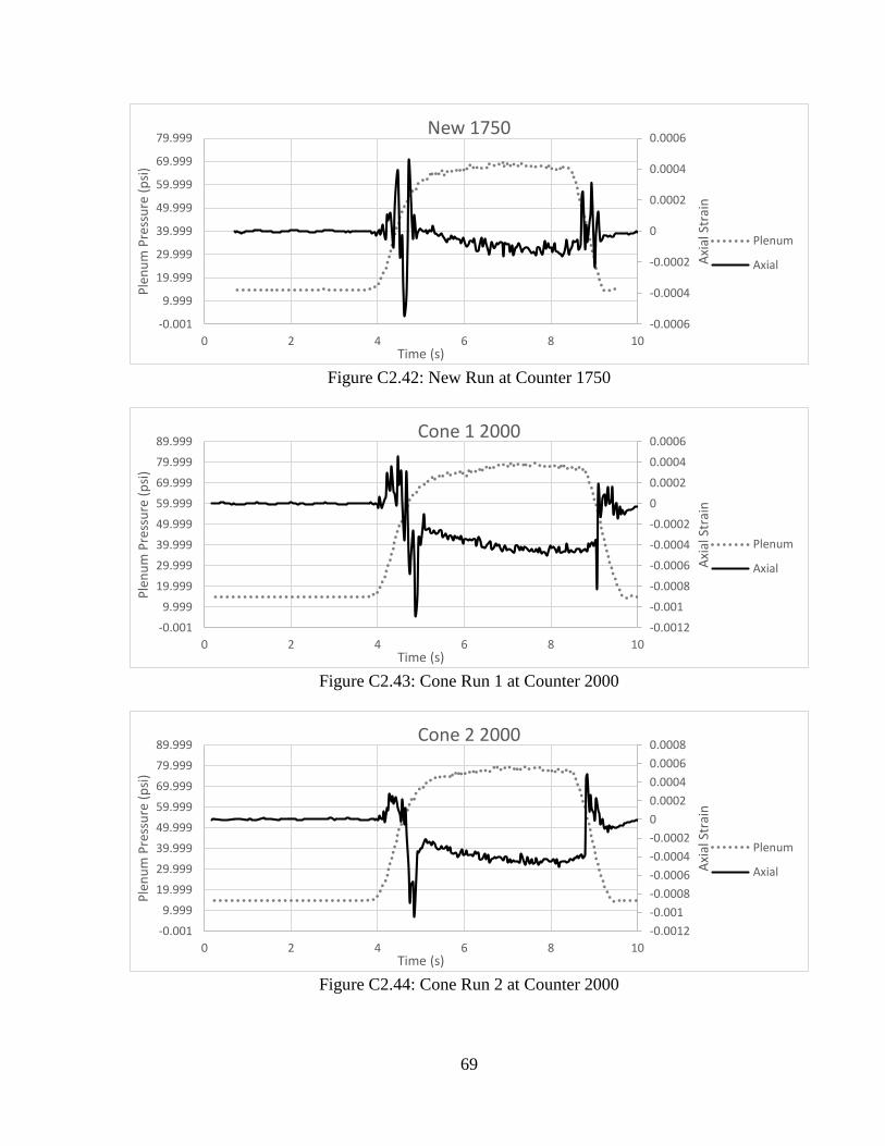
69
Figure C2.42: New Run at Counter 1750
Figure C2.43: Cone Run 1 at Counter 2000
Figure C2.44: Cone Run 2 at Counter 2000
-0.0006
-0.0004
-0.0002
0
0.0002
0.0004
0.0006
-0.001
9.999
19.999
29.999
39.999
49.999
59.999
69.999
79.999
0 2 4 6 8 10
Axi
al S
trai
n
Ple
nu
m P
ress
ure
(p
si)
Time (s)
New 1750
Plenum
Axial
-0.0012
-0.001
-0.0008
-0.0006
-0.0004
-0.0002
0
0.0002
0.0004
0.0006
-0.001
9.999
19.999
29.999
39.999
49.999
59.999
69.999
79.999
89.999
0 2 4 6 8 10
Axi
al S
trai
n
Ple
nu
m P
ress
ure
(p
si)
Time (s)
Cone 1 2000
Plenum
Axial
-0.0012
-0.001
-0.0008
-0.0006
-0.0004
-0.0002
0
0.0002
0.0004
0.0006
0.0008
-0.001
9.999
19.999
29.999
39.999
49.999
59.999
69.999
79.999
89.999
0 2 4 6 8 10
Axi
al S
trai
n
Ple
nu
m P
ress
ure
(p
si)
Time (s)
Cone 2 2000
Plenum
Axial
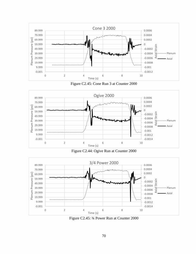
70
Figure C2.45: Cone Run 3 at Counter 2000
Figure C2.44: Ogive Run at Counter 2000
Figure C2.45: ¾ Power Run at Counter 2000
-0.0012
-0.001
-0.0008
-0.0006
-0.0004
-0.0002
0
0.0002
0.0004
0.0006
-0.001
9.999
19.999
29.999
39.999
49.999
59.999
69.999
79.999
89.999
0 2 4 6 8 10
Axi
al S
trai
n
Ple
nu
m P
ress
ure
(p
si)
Time (s)
Cone 3 2000
Plenum
Axial
-0.0014
-0.0012
-0.001
-0.0008
-0.0006
-0.0004
-0.0002
0
0.0002
0.0004
0.0006
-0.001
9.999
19.999
29.999
39.999
49.999
59.999
69.999
79.999
89.999
0 2 4 6 8 10
Axi
al S
trai
n
Ple
nu
m P
ress
ure
(p
si)
Time (s)
Ogive 2000
Plenum
Axial
-0.0014
-0.0012
-0.001
-0.0008
-0.0006
-0.0004
-0.0002
0
0.0002
0.0004
0.0006
-0.001
9.999
19.999
29.999
39.999
49.999
59.999
69.999
79.999
89.999
0 2 4 6 8 10
Axi
al S
trai
n
Ple
nu
m P
ress
ure
(p
si)
Time (s)
3/4 Power 2000
Plenum
Axial
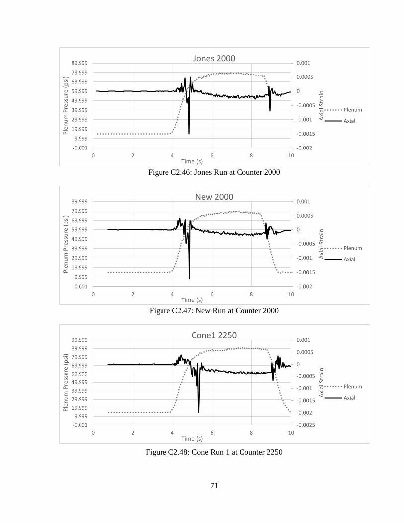
71
Figure C2.46: Jones Run at Counter 2000
Figure C2.47: New Run at Counter 2000
Figure C2.48: Cone Run 1 at Counter 2250
-0.002
-0.0015
-0.001
-0.0005
0
0.0005
0.001
-0.001
9.999
19.999
29.999
39.999
49.999
59.999
69.999
79.999
89.999
0 2 4 6 8 10
Axi
al S
trai
n
Ple
nu
m P
ress
ure
(p
si)
Time (s)
Jones 2000
Plenum
Axial
-0.002
-0.0015
-0.001
-0.0005
0
0.0005
0.001
-0.001
9.999
19.999
29.999
39.999
49.999
59.999
69.999
79.999
89.999
0 2 4 6 8 10
Axi
al S
trai
n
Ple
nu
m P
ress
ure
(p
si)
Time (s)
New 2000
Plenum
Axial
-0.0025
-0.002
-0.0015
-0.001
-0.0005
0
0.0005
0.001
-0.001
9.999
19.999
29.999
39.999
49.999
59.999
69.999
79.999
89.999
99.999
0 2 4 6 8 10
Axi
al S
trai
n
Ple
nu
m P
ress
ure
(p
si)
Time (s)
Cone1 2250
Plenum
Axial
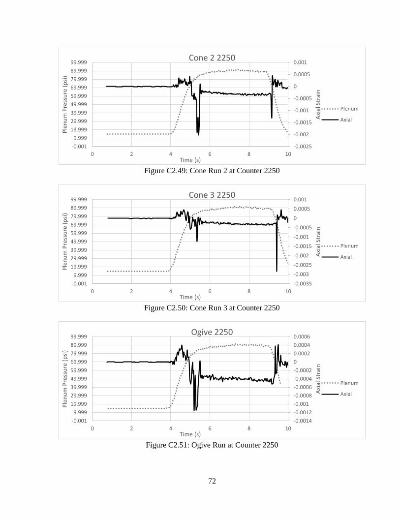
72
Figure C2.49: Cone Run 2 at Counter 2250
Figure C2.50: Cone Run 3 at Counter 2250
Figure C2.51: Ogive Run at Counter 2250
-0.0025
-0.002
-0.0015
-0.001
-0.0005
0
0.0005
0.001
-0.001
9.999
19.999
29.999
39.999
49.999
59.999
69.999
79.999
89.999
99.999
0 2 4 6 8 10
Axi
al S
trai
n
Ple
nu
m P
ress
ure
(p
si)
Time (s)
Cone 2 2250
Plenum
Axial
-0.0035
-0.003
-0.0025
-0.002
-0.0015
-0.001
-0.0005
0
0.0005
0.001
-0.001
9.999
19.999
29.999
39.999
49.999
59.999
69.999
79.999
89.999
99.999
0 2 4 6 8 10
Axi
al S
trai
n
Ple
nu
m P
ress
ure
(p
si)
Time (s)
Cone 3 2250
Plenum
Axial
-0.0014
-0.0012
-0.001
-0.0008
-0.0006
-0.0004
-0.0002
0
0.0002
0.0004
0.0006
-0.001
9.999
19.999
29.999
39.999
49.999
59.999
69.999
79.999
89.999
99.999
0 2 4 6 8 10
Axi
al S
trai
n
Ple
nu
m P
ress
ure
(p
si)
Time (s)
Ogive 2250
Plenum
Axial
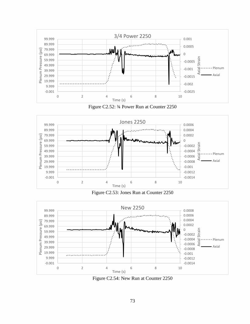
73
Figure C2.52: ¾ Power Run at Counter 2250
Figure C2.53: Jones Run at Counter 2250
Figure C2.54: New Run at Counter 2250
-0.0025
-0.002
-0.0015
-0.001
-0.0005
0
0.0005
0.001
-0.001
9.999
19.999
29.999
39.999
49.999
59.999
69.999
79.999
89.999
99.999
0 2 4 6 8 10
Axi
al S
trai
n
Ple
nu
m P
ress
ure
(p
si)
Time (s)
3/4 Power 2250
Plenum
Axial
-0.0014
-0.0012
-0.001
-0.0008
-0.0006
-0.0004
-0.0002
0
0.0002
0.0004
0.0006
-0.001
9.999
19.999
29.999
39.999
49.999
59.999
69.999
79.999
89.999
99.999
0 2 4 6 8 10
Axi
al S
trai
n
Ple
nu
m P
ress
ure
(p
si)
Time (s)
Jones 2250
Plenum
Axial
-0.0014
-0.0012
-0.001
-0.0008
-0.0006
-0.0004
-0.0002
0
0.0002
0.0004
0.0006
0.0008
-0.001
9.999
19.999
29.999
39.999
49.999
59.999
69.999
79.999
89.999
99.999
0 2 4 6 8 10
Axi
al S
trai
n
Ple
nu
m P
ress
ure
(p
si)
Time (s)
New 2250
Plenum
Axial