EXPERIMENTS ON OPTIMIZING THE PERFORMANCE OF …ppl14.pdf · July 27, 2014 16:17 WSPC/INSTRUCTION FILE paper Experiments on Optimizing Performance of Stencil Codes with SPL Conqueror

July 27, 2014 16:17 WSPC/INSTRUCTION FILE paper

Parallel Processing Lettersc© World Scientific Publishing Company

EXPERIMENTS ON OPTIMIZING THE PERFORMANCE OF

STENCIL CODES WITH SPL CONQUEROR

ALEXANDER GREBHAHN† and SEBASTIAN KUCKUK‡ and CHRISTIAN SCHMITT‡ andHARALD KOSTLER‡ and NORBERT SIEGMUND† and SVEN APEL† and

FRANK HANNIG‡ and JURGEN TEICH‡

† University of Passau, Passau, Germany‡ Friedrich-Alexander University of Erlangen-Nurnberg (FAU), Erlangen, Germany

Received April 2014

Revised July 2014

Communicated by Guest Editors

ABSTRACT

A standard technique for numerically solving elliptic partial differential equations onstructured grids is to discretize them, and, then, to apply an efficient geometric multi-grid

solver. Unfortunately, finding the optimal choice of multi-grid components and parametersettings is challenging and existing auto-tuning techniques fail to explain performance-

optimal settings. To improve the state of the art, we explore whether recent work on

optimizing configurations of product lines can be applied to the stencil-code domain. Inparticular, we extend the domain-independent tool SPL Conqueror in an empirical study

to predict the performance-optimal configurations of three geometric multi-grid stencil

codes: a program using HIPAcc, the evaluation prototype HSMGP, and a program usingDUNE. For HIPAcc, we reach an prediction accuracy of 96 %, on average, measuring

only 21.4 % of all configurations; we predict a configuration that is nearly optimal after

measuring less than 0.3 % of all configurations. For HSMGP, we predict performance withan accuracy of 97 % including the performance-optimal configuration, while measuring

3.2 % of all configurations. For DUNE, we predict performance of all configurations with

an accuracy of 86 % after measuring 3.3 % of all configurations. The performance-optimalconfiguration is within the 0.5 % configurations predicted to perform best.

Keywords: Stencil computations, parameter optimization, auto-tuning, product lines,

SPL Conqueror, multi-grid methods

1. Introduction

In many areas of computation, such as climate forecasts and complex simulations,

large linear and non-linear systems have to be solved. Multi-grid methods [1, 2]

represent a popular class of solutions for systems exhibiting a certain structure.

For instance, from the discretization of partial differential equations (PDEs) on

structured grids, sparse and symmetric positive definite system matrices arise (see

Briggs et al. [3] and Trottenberg et al. [4] for a comprehensive overview on multi-

grid methods). Algorithmically, most of the multi-grid components are functions

1


2 Parallel Processing Letters

that sweep over a computational grid and perform nearest-neighbor computations.

Mathematically, these computations are linear-algebra operations, such as matrix-

vector products. Since the matrices are sparse and often contain similar entries in

each row, they can be described by a stencil, where one stencil represents one row

in the matrix.

A multi-grid algorithm consists of several components and traverses a hierarchy

of grids several times until the linear system is solved up to a certain accuracy. The

components as well as their parameters, for instance, how often a certain compo-

nent is applied on each level, are highly problem and platform dependent. That

is, depending on the hardware and the application scenario, some parameter set-

tings perform faster than others. This variability gives rise to a considerable number

of configuration options to customize multi-grid algorithms and the corresponding

code.

Selecting configuration options (i. e., specifying a configuration) to maximize

performance is an essential activity in exascale computing [5]. If a non-optimal

configuration is used, the full computational power may not be exploited, lead-

ing to increased costs and time requirements. Identifying the performance-optimal

configuration is a complex task: Measuring the performance of all configurations

to determine the fastest one does not scale because the number of configurations

grows exponentially with the number of configuration options, in the worst case.

Alternatively, we can use domain knowledge to identify the fastest configuration.

However, domain knowledge is not always available, and domain experts are rare

and expensive. Moreover, recent work shows that problems can become easily such

complex that even domain experts cannot determine the best configuration [6, 7].

In product-line engineering, different approaches have been developed to tackle

the problem of finding optimal configurations in a possibly exponential configuration

space [8, 9, 10, 11]. The idea is to measure some configurations of a program and

predict the performance of all other configurations (e. g., using machine-learning

techniques).

Our goal is to find out whether existing product-line techniques can be applied

successfully to automatic stencil-code optimization. In particular, we use and extend

the tool SPL Conqueror by Siegmund et al. [10] to determine the performance

influence of individual configuration options of stencil-code implementations. The

general idea is to determine the performance influence of individual configuration

options first, and to consider interactions between them subsequently. We propose

a sampling heuristic with which we learn the performance contribution of numerical

options (i.e., options that have a numerical value range, such as number of smoothing

steps) with the help of functions learning, which is a novel contribution to SPL

Conqueror.

We conducted an empirical study involving three case studies from the stencil

domain. One of the systems investigated is a geometric multi-grid implementation

using HIPAcc [12], a domain-specific language and compiler targeting GPU acceler-

ators and low-level programming languages. The second system is a prototype of a


Experiments on Optimizing Performance of Stencil Codes with SPL Conqueror 3

highly scalable geometric multi-grid solver (HSMGP) developed for testing various

algorithms and data structures on high-performance computing systems [13] such

as the JuQueen at the Julich Supercomputing Centre, Germany. The last system

is a geometric multi-grid solver implementation using the numerics environment

DUNEa.

Overall, we make the following contributions: We demonstrate that SPL Con-

queror can be applied to the stencil domain to identify optimal configurations after

performing only a small number of measurements. With more measurements, we can

predict the performance of all configurations with an accuracy of about 97 %, on

average, in two of three cases; in two cases, we are able to identify the performance-

optimal configuration or a configuration causing only a small performance overhead.

In the third case, the best configuration is within the range of 0.5 % configurations

predicted to be best. This article is a revised and extended version of our previ-

ous HiStencils workshop paper [14]. Compared to the earlier version, we included a

third case study (the implementation using DUNE), performed more measurements,

adjusted the measurement setup, and included more discussions.

2. Preliminaries

In this section, we present the preliminaries of our approach of finding performance-

optimal stencil-code configurations. As the approach has its roots in the product-line

domain, we introduce the respective terminology and provide background informa-

tion on how to model variability.

2.1. Feature Models and Extended Feature Models

In the product-line domain, configuration options of variable systems are often called

features [15]. As features may depend on or exclude each other, feature models are

used to describe their valid combinations [16]. A feature model describes relation-

ships among the features of a configurable system by grouping them and introducing

a parent-child relationship (if the child feature is selected the parent feature must

be selected, too). We present the feature models of our three subject systems in

Figure 1a–c.

In general, a feature can either be mandatory (i. e., required in all configurations

in which its parent feature is selected), optional, or be part of an OR group or an

XOR group. If the parent feature of a group is selected, exactly one feature of

an XOR group and, at least, one of an OR group must be selected. Additionally,

one can define arbitrary propositional formulas to further constrain variability. For

example, one feature may imply or exclude another feature or set of features.

Standard feature models can express features with two states only, indicating

the presence or absence of the corresponding feature in a configuration; We refer to

ahttp://www.dune-project.org/



these features as Boolean features. In Figure 1 and 2, Boolean features are framed

with a solid box.

However, having Boolean features only is insufficient when modeling variability

of multi-grid systems, because there are configuration options, here called numerical

features, that can take more than two states. For example, we need to specify the

number of pre-smoothing steps within a multi-grid solver, which is a numerical value

within the range of 0 and 6 (see Figure 1b). Consequently, numerical features have

a value domain (i. e., the specified value range of the feature) and, additionally,

a default value. For instance, the numerical feature Padding (cf. Figure 1a) has

the value domain Integer, and the range is between 0 and 512 with a step size of

32. The default value is 0. In Figure 1 and 2, numerical features are denoted with

dashed boxes. Alternatively, we can model a numerical feature as a set of Boolean

features that discretize the value range, such that one Boolean feature represents

one value of the numerical feature. However, this approach leads to an increasing

number of Boolean features (see Figure 2) and hinders interpolating a function over

the whole value range, to predict influence of unseen values of a numerical feature

(see Section 4).

2.2. Predicting the Performance of Configurable Systems

To predict the performance of the configurations of a configurable systems, we de-

veloped SPL Conqueror, which quantifies the influence of individual features on

performance (and on other non-functional properties) [10, 17]. To quantify the in-

fluence, we use the machine-learning approach Forward Feature Selection [18], which

quantifies based on a test set (i.e., a set of measured configurations) the influences of

all features on performance. The main research question is, however, how to select

the test set. That is, which configurations should we measure to learn a model that

accurately predicts performance of all configurations. To this end, we developed in

previous work several sampling heuristics, which we explain in the following.

The first heuristic, feature-wise (FW), aims at feature coverage. We select config-

urations in which only a single feature is selected to measure the feature’s influence

in isolation (actually, based on the smallest possible configuration that represents

a valid, running program). We repeat this for each feature of the feature model.

For example, if we want to determine how the selection of feature Local Memory

of the HIPAcc framework influences the performance, we measure the configuration

in which all features but Local Memory are deselected. To obtain a valid configura-

tion, we additionally have to select mandatory features, such as API and Blocksize.

As a result of this sampling process, the test set contains a configuration for each

Boolean feature (excluding mandatory features), with which we can determine the

influence of the corresponding feature.

However, since we have no two configurations where multiple features are se-

lected, the predicted performance of an unseen configuration may not always match

the actual performance, because features may influence each other. This influence



HSMGP

post-smoothing[0,…,6]

3

pre-smoothing[0,…,6]

3

sum (pre-smoothing, post-smoothing) > 0

(b)

(a)

coarse grid solver

IP_CG IP_AMGRED_AMG

smoother

GSACGSJac BSRBGS RBGSAC

Number of Cores[64,256,1024,4096]

64

HIPAcc

API

CUDA

Texture Memory

OpenCL Linear2D Array2D

Padding[0,32,…,512]

0

Pixels per Thread [1,2,3,4]

1

¬(OpenCL ˄ Linear1D)¬(OpenCL ˄ Linear2D)

¬(OpenCL ˄ Ldg)

Blocksize

¬(Local Memory ˄ 1024x1 ˄ Pixel Per Thread = 2)¬(Local Memory ˄ 32x32 ˄ Pixel Per Thread = 3)¬(Local Memory ˄ 64x16 ˄ Pixel Per Thread = 3)

Local Memory

32x1 64x16

128x1 128x2 128x4 128x8 256x4 512x1 512x2 1024x1

Ldg

32x2 32x4 64x2 64x8

256x1 256x2

(Array2D Padding = 0)




¬(Local Memory ˄ 1024x1 ˄ Pixel Per Thread = 4)

32x1632x8 64x432x32 64x1

Linear1D

Dune MGS

post-smoothing[0,…,6]

3

pre-smoothing[0,…,6]

3

sum (pre-smoothing, post-smoothing) > 0

(c)

preconditioner

GS

solver

CG LoopBicGSTAB Gradient

Number of Cells[50,…,55]

50

SOR

Mandatory

Optional

XOR groupOR group

Fig. 1. Feature models for the three target systems: (a) HIPAcc, (b) HSMGP, and (c) Dune MGS.

(a)

SystemX

[0,1,…,n]0

(b)System

X0 X1 Xn...

Fig. 2. Different modeling strategies of numerical features. (a) Feature model with the numerical

feature X and (b) the same feature model with the numerical feature modeled as a set of discretizedBoolean features in an XOR group.

on performance arises due to feature interactions [10]. For example, effects of chang-

ing the used Texture Memory can vary based on the current API (see Figure 1a).

Furthermore, interactions between more than two features are possible. To take

these interactions of different orders (i. e., the number of features causing a perfor-

mance interaction) into account, Siegmund et al. propose three further sampling



heuristics [10].

The pair-wise heuristic (PW) considers interactions between all pairs of inter-

acting features. However, since all features can possibly interact with each other, we

first need to determine which features actually interact. First, we measure for each

feature an additional configuration in which we maximize the number of selected

features. The idea behind is to maximize the possibility of observing a performance

interaction. Only if the measured performance of this configuration does not corre-

spond to the predicted performance, which does not take interactions into account,

we know that features of this configuration interact. For a more detailed discussion,

we refer to [19]. Knowing the features that interact, we need to determine which

exact combination of those features actually cause a performance difference. Hence,

we measure additional configurations in which we combine each pair of interacting

features (i.e., the pair-wise sampling heuristic). The higher-order heuristic (HO)

specifies configurations to be measured to detect interactions of the order of two

(i.e., when three features cause an interaction). Lastly, in some customizable pro-

grams there are features, called hot-spot features, that are responsible for most of

the interactions. The hot-spot heuristic (HS) further extends the test set by those

configurations in which a previously identified hot-spot feature is selected. The idea

is to detect more relevant interactions with only few more measurements. The three

heuristics build on each other and on the FW heuristic. As a consequence, the

HS heuristic uses all measurements already performed by the FW, PW, and HO

heuristic.

All heuristics presented so far sample the configuration space of Boolean features

only. As a consequence, it is not possible to incorporate numerical features directly.

Instead, numerical features have to be modeled as discretized sets of Boolean fea-

tures (see Figure 2) leading to a substantially increased number of measurements.

To overcome this limitation, we propose a novel function-learning heuristic (FL).

The basic idea is to learn performance-contribution functions for each numerical

feature. Since each numerical feature can have a different performance influence

on different Boolean features, we learn a function for each pair of numerical and

Boolean feature. The structure of the performance function (e.g., the polynomial

degree) has to be given by a domain expert or obtained by machine learning. Conse-

quently, a feature model with n Boolean features and m numerical features requires

n · m functions. To learn these performance-contribution functions, we sample in

the range of the numerical feature, based on its expected polynomial degree and

measure the performance of the corresponding configurations. For example, when

expecting a quadratic contribution function for feature pre-smoothing of HSMGP,

we measure three configurations for this numerical feature. In the first configuration,

the value of this feature is 0, in the second 3, and in the last one 6. When sampling a

single numerical feature, we keep the remaining numerical features constant, using

their default values. To learn the different performance-contribution functions of

a numerical feature (a function for each feature), we combine this sampling strat-



egy with the FW heuristic. After measurement, we use least-squares regression to

determine the contribution of the numerical feature.

3. Experiments

We conducted a series of experiments to evaluate whether the approach taken by

SPL Conqueror is feasible for predicting performance of geometric multi-grid-solver

configurations. To this end, we define the following research questions:

• Q1: What is the prediction accuracy and measurement effort of the heuris-

tics FW, PW, HO, HS, and FL?

• Q2: What is the performance difference between the optimal configuration

and the configuration predicted to perform best by the heuristics?

3.1. Experimental Setup and Procedure

To answer the research questions, we selected three multi-grid solver implementa-

tions from different application domains, which we describe in the Sections 3.2–3.4.

Note that we consider only the execution time in our evaluation, not compilation

time (compilation time can usually be neglected in production runs).

Each experiment consists of two phases. In the first phase, we measure a subset of

configurations of the subject systems and determine the contributions of individual

features, feature interactions, and numerical features; the measured configurations

are selected by the individual sampling heuristics (FW, PW, HO, HS, FL). In

the second phase, the performance of all configurations is predicted, based on the

contributions determined before. To calculate the prediction accuracy of the second

phase, we additionally measured all configurations of all systems, essentially a Brute

Force (BF) approach, and compared the actual times to the times predicted when

using the heuristics. The mean relative error rate e is calculated for each heuristic,

as follows:

e =1

n

∑0≤i<n

|tmeasured

i − tpredicted

i |tmeasuredi

,

where n is the number of configurations of the subject system. Additionally, we de-

termine the performance difference between the performance-optimal configuration,

as determined by BF, and the configuration predicted to perform best by the heuris-

tics. For evaluation, we performed exhaustive measurements on different hardware

systems and kept the hardware constant for each subject system.

3.2. HIPAcc

HIPAcc, the Heterogeneous Image Processing Acceleration Frameworkb, generates

efficient low-level code from a high-level embedded domain-specific language [20].

bhttp://hipacc-lang.org



During compilation, HIPAcc optimizes the computational kernels by exploiting do-

main and hardware knowledge. The tested geometric multi-grid code solves a finite

difference discretization of the Poisson equation on a rectangular grid.

HIPAcc has a built-in list of supported hardware platforms allowing the target ar-

chitecture to be selected at compile time. This variability, however, is exploited only

for the built-in auto-tuning process preventing the generation of code unsuitable for

the targeted device. In our experiments, we did not vary the hardware device. We

illustrate the features we considered with the feature model in Figure 1a; a more

complete description of the HIPAcc configuration space can be found in Membarth

et al. [21]. As the API used for interaction with the device has to be specified,

we modeled it as an XOR group. Another XOR group is the memory layout used,

donated by the feature Texture Memory. Additionally, Local Memory is an optional

feature toggling the use of another memory type. The integer value Padding, mod-

eled as a numerical feature, may be set to optimize the memory layout. Furthermore,

the integer value Pixels per Thread, denoting how many pixels are calculated per

thread, can be varied. For further details of these configuration options, we refer to

Grebhahn et al. [14]. Finally, we used different block sizes within our experiments,

which are modeled as an XOR group, too.

We performed all measurements of the HIPAcc system on an nVidia Tesla K20

card with 5GB RAM and 2496 cores. As an indicator for performance, we measure

the time to compute the solution.

3.3. Highly Scalable MG Prototype (HSMGP)

HSMGP is a prototype code for benchmarking Hierarchical Hybrid Grids

(HHG) [22, 23], data structures, algorithms, and concepts [13]. It was designed

to run on large scale systems, such as JuQueen, a Blue Gene/Q system, located

at the Julich Supercomputing Centre, Germany. In its current form, it solves a fi-

nite differences discretization of Poisson’s equation on a general block-structured

domain.

The variability of HSMGP is illustrated in Figure 1b. In particular, the solver

provides different smoothers, represented by an XOR group. The second customiz-

able algorithmic component is the coarse-grid solver. The resulting choices are an

in-place conjugate gradient (IP CG), an in-place algebraic multi-grid (IP AMG),

and an algebraic multi-grid with data reduction (RED AMG), which are also mod-

eled in an XOR group.

Furthermore, in our experiments, we can choose the number of pre- and post-

smoothing steps, both of which we limit to integer values between 0 and 6; the

default value is set to 3 (see Grebhahn et al. [14], for further details). We performed

weak scaling experiments using a varying number of nodes. In detail, we utilized

64, 256, 1024, and 4096 nodes, where 64 is the default value.

Since the configuration space is small compared to a full model of HSMGP,

we are able to measure all configurations (BF), which is necessary to determine



accuracy of the heuristics. We performed all of the experiments of this system on

the JuQueen system at the Julich Supercomputing Centre, Germany. Although the

application scales up to the whole machine (458 752 cores) [13], we used only a

smaller test case to ensure reproducibility and cost effectiveness (in terms of CPU

hours).

We decided to evaluate the average time needed to perform one V-cyclec, in-

stead of the total time. As it is not possible to identify the performance-optimal

configuration of a system in considering the time needed to perform one cycle only,

we multiply the predicted time of one cycle with the measured number of cycles for

the configurations of the HSMPG system. As an alternative, the number of cycles

needed, can also be predicted using local Fourier analysis [4].

3.4. Dune MGS

The third subject system is a geometric multi-grid implementation based on

DUNEd. DUNE is a framework for solving PDEs with grid-based methods. The

selected implementation solves a finite element discretization of Poisson’s equation

on a structured grid.

The variability we consider is presented in Figure 1c. There are two alternative

preconditioners and four alternative solvers. The preconditioners and solvers are

provided by the DUNE framework. In addition, we vary the pre- and post-smoothing

steps, which we limit to integer values within the range of 0 to 6, using 3 as default

value. We performed the experiments with a different number of cells, defining the

grid size.

All measurements for this system are performed on an Dell OptiPlex-9020 with

an Intel i5-4570 Quad Code and 32 GB RAM, running Ubuntu 13.4. For this system,

we measure the time to compute the solution as an indicator for performance.

4. Results

The experimental results for the three subject systems are given in Table 1. Next,

we describe them in detail. The BF approach acts as a base line for the number

of measurements. Regarding research question Q1 (prediction accuracy and mea-

surement effort), we present the number of needed measurements of the different

heuristics, the fault distribution, the average error rate, the standard deviation, and

the median error rate of the predictions. For the research question Q2 (performance

difference between the optimal configuration and the configuration predicted to per-

form best), we computed the absolute and the percentage share difference between

the measured performance of the optimal configuration and the measured perfor-

mance of the configuration predicted to perform best. Besides, we computed the

cA V-cycle is an iteration traversing a hierarchy of grids.dhttp://www.dune-project.org/dune.html



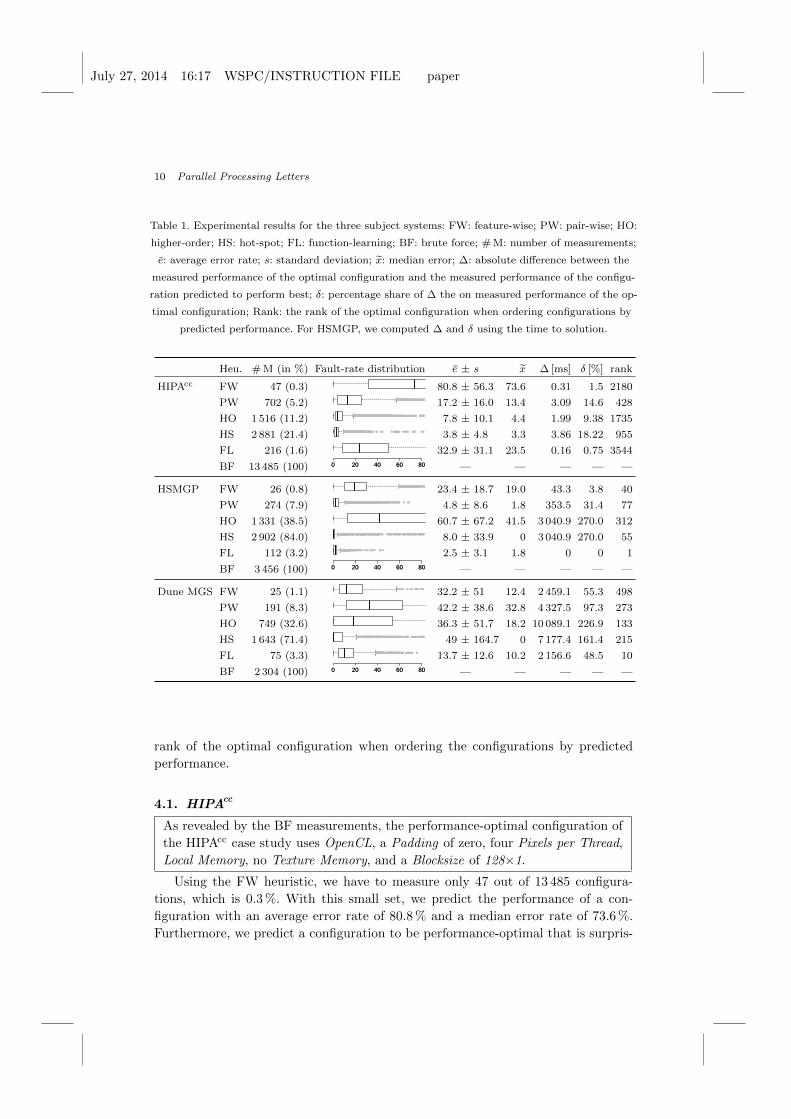
Table 1. Experimental results for the three subject systems: FW: feature-wise; PW: pair-wise; HO:

higher-order; HS: hot-spot; FL: function-learning; BF: brute force; # M: number of measurements;

e: average error rate; s: standard deviation; x: median error; ∆: absolute difference between the

measured performance of the optimal configuration and the measured performance of the configu-

ration predicted to perform best; δ: percentage share of ∆ the on measured performance of the op-

timal configuration; Rank: the rank of the optimal configuration when ordering configurations by

predicted performance. For HSMGP, we computed ∆ and δ using the time to solution.

Heu. # M (in %) Fault-rate distribution e ± s x ∆ [ms] δ [%] rank

HIPAcc FW 47 (0.3) 80.8 ± 56.3 73.6 0.31 1.5 2180

PW 702 (5.2) ● ●● ●●●● ●● ●● ●● ●● ● ●●● ● ●●● ●● ●● ● ●● ● ●●●●●● ●●●● ●●●● ●● ●●● ● ●● ●● ●● ●●● ●● ●● ●●●●● ● ●●● ●●● ●● ● ●●● ● ●● ●● ●● ●●●●● ●● ●●●● ●● ●●● ●●●●●●● ●●●● ●●● ● ●●●●●●● ●● ●●● ●●●● ●●● ●● ●●● ●● ●●● ●● ●●●●●● ●●●●●●●●●●●●●● ●●● ●●● ●●●●● ●●●●●● ● ●●●●●● ●● ●●● ● ●●●●● ● ●●●●●●●●●●●● ●●●●● ●●●●●●●●●● ●●●●●●● ●●● ●● ● ●●● ●●● ●● ●●● ● ●● ● ●● ●●●●●● ●● ●● ●●●●●● ●● ●● ●● ● ●●●●●●●● ●●● ●●●●● ●●● ●● ● ●● ● ●● ●● ●● ●●●● ●●●● ●● ●●●● ●● ●● ● ●●● ● ●● ●●●● ● ●●● ●●●●●●●●●●●●●● ●●● ● ●●● ●●●●●●●●●●●●●●●●●●●●●●●●●●●●●●●●● ●●●●●●●●●●●●●●●●●●●●●●●●●●●●●●●●●●●●●●●●●● ●●●●●● ● ●● ●●●● ●● ●● ●● ●● ● ●●● ● ●●● ●● ●● ● ●● ● ●●●●●● ●●●● ●●●● ●● ●●● ● ●● ●● ●● ●●● ●● ●● ●●●●● ● ●●● ●●● ●● ● ●●● ● ●● ●● ●● ●●●●● ●● ●●●● ●● ●●● ●●●●●●● ●●●● ●●● ● ●●●●●●● ●● ●●● ●●●● ●●● ●● ●●● ●● ●●● ●● ●●●●●● ●●●●●●●●●●●●●● ●●● ●●● ●●●●● ●●●●●● ● ●●●●●● ●● ●●● ● ●●●●● ● ●●●●●●●●●●●● ●●●●● ●●●●●●●●●● ●●●●●●● ●●● ●● ● ●●● ●●● ●● ●●● ● ●● ● ●● ●●●●●● ●● ●● ●●●●●● ●● ●● ●● ● ●●●●●●●● ●●● ●●●●● ●●● ●● ● ●● ● ●● ●● ●● ●●●● ●●●● ●● ●●●● ●● ●● ● ●●● ● ●● ●●●● ● ●●● ●●●●●●●●●●●●●● ●●● ● ●●● ●●●●●●●●●●●●●●●●●●●●●●●●●●●●●●●●● ●●●●●●●●●●●●●●●●●●●●●●●●●●●●●●●●●●●●●●●●●● ●●●●●● 17.2 ± 16.0 13.4 3.09 14.6 428

HO 1 516 (11.2) ●●● ●●●●●●●●●●●●● ●●● ●●●●● ●●●●●●●●● ●●● ●●●●● ●●●● ●●●● ●●●● ●●●●● ●● ●● ●● ●●●●● ● ●●● ●●● ●● ●●●●●●●● ●●●●●●●●● ●● ●●● ●● ●●●● ●● ●● ●● ● ●● ●● ●●●●●● ●●●●● ●● ● ●●●●● ●●● ●●● ● ●● ●●● ●● ●●●● ●●● ●●●● ● ●●● ●●● ●●●●● ●●●●●●●● ●●●● ●●●●●●●● ●●● ● ●●● ●●●●● ●● ●●●●● ●●● ●●●●● ●●● ●● ●●●●● ● ●●●● ●●●●● ●● ● ●●●●● ●● ●● ●●● ●●● ●● ●● ●● ●●●● ●●●●●●● ●● ●● ●●● ●●●●● ●●● ●●●● ●● ●● ●● ● ●●●● ●●●●● ●●● ●●● ●● ●● ●● ●● ●●●●●●● ● ● ●● ● ●●●●●● ●●● ●● ●●●●●●●●● ●● ● ●●●●●● ●●●●●● ● ●● ●● ●●●● ●●●●● ●●●●● ●●●● ●●● ●● ● ●● ●●● ●●●● ●●● ●●●●●●●●●●●● ●●●● ●● ●●●●●● ●●●●●● ●●●● ●●●● ●●● ●● ●●●● ●●●●● ●●●● ●●●●●● ●●● ● ●● ●●● ● ●●●● ●● ●●● ●●●● ●●● ●●●●●●● ●●●●●●●● ●●●● ●●●●●●●●●● ●●● ●●●●●● ●●●● ● ●●●● ●●●●● ●●● ● ●●●● ● ●●● ●● ●● ●●● ●●●● ●●●● ●● ● ●● ●● ●●● ●●●● ●●●●●● ●● ●● ●●● ●● ●●●● ● ● ●● ●● ●●●●●●● ●● ●●● ●● ●●●● ●● ●●● ● ●●● ●●●● ●●●● ●● ●● ●● ●●●●●● ●●● ●● ● ●● ● ●●●●● ●●● ●● ●●●●●● ●● ● ● ●● ● ●● ●● ● ●● ● ●●● ● ●● ●●●● ●●●● ●● ●● ●● ●●●●● ●● ●● ●● ●●● ●●● ●● ●●●●●● ●●● ●●●● ●●● ● ● ●●●●● ● ● ●● ●●● ●●●●● ● ●● ●● ●●● ●●●● ●● ●●● ●●● ●●● ●● ●●●●●● ●●●●●●● ●● ●● ●●●●● ●●● ●● ●●● ●● ●●●●●●●●● ●●●● ●●●● ●● ●● ●● ●●●● ●●● ●● ●● ●● ● ●● ●● ●● ● ●● ●●● ●● ●● ●● ●● ●● ●● ● ●●●●●●●● ●●● ●●●●● ●●●●● ●●● ●● ●●● ●●●● ● ●● ●●● ● ●● ●●● ● ●● ●● ●● ●●● ● ●● ●●● ●●●●● ●●●● ●●●●●● ●●●●●● ●● ●●●● ●●●● ●● ●●●●●● ●● ● ●●●●●● ●●●● ●● ●● ●●●● ● ●●● ● ●●●●●●●●●● ●● ●● ● ●●● ● ●● ●● ●●● ●● ●●●● ●●● ●● ●●●●● ●● ●●●● ● ●●● ●●●●● ●● ●●●●●●● ●●●●●●● ●● ●● ●● ●● ●●●●● ● ●●●●●●●● ●● ●● ●● ●●●●● ● ●●● ●● ● ●●●● ●●● ●●●● ●●●● ●●●● ●●●● ●● ●●● ●●● ● ● ●●●● ●●●● ●● ●● ●● ● ●● ●●● ●● ●● ●●●● ●●●●●● ●● ●●● ● ●● ●●●● ●●●●●●● ● ●●●●●●● ●●●●●● ● ●●●● ●● ●● ●● ●●●●●● ●●● ●●● ●●● ●●●●●● ●●●●● ●● ●● ●●●●●●● ●● ●● ●● ●●● ● ●●● ●●●●●● ● ●● ●●● ● ● ●● ●●●●●● ● ●●●●● ●●● ●●●●●●●●●● ●●●● ●●● ●● ●●● ●● ●●●● ●●●●●●●●● ●●●● ● ●●● ●●●●●●●●● ●●● ●● ●●● ● ●● ●●●● ●● ●●●●● ●●●● ●●● ●●●●● ●● ●● ●●●●●● ●●● ●●●● ● ● ●●●● ● ● ●●●● ●●●● ●●●●●●●● ●● ●●●● ●● ●●● ●●● ●●●● ●● ●●●● ● ●● ●●●●●● ●● ●●●●●●●●● ●●●●●●●●●●●●●●●● ●●● ●●●● ●●●●● ●●● ●●●●●● ●●●●●●●●●●●●●● ●●● ●●● ●●●● ●● ●●● ●●●● ●●●●●●●●●●● ●●●● ●●● ●● ●●●● ● ●●●●● ● ● ●●● ● ●●●● ●●●●●●●● ●● ●● ●● ● ●●● ●● ●● ●●●●●● ●● ●●●●●●● ●● ●●● ●● ●●● ●● ●●● ●●●●●● ●● ●●●● ●●● ●●● ●●●●●●● ●●●●● ●●●● ●● ●●●●●● ●●● ●●●●● ●●●●●●●●●●●●●●●●●●●● ● ●●●●●● ●●● ●●● ●● ●● ●●●●●● ●● ●●● ●● ●●● ●●● ●●●● ●●●●●●●● ●●● ●●●●●●●●●●●●● ●●● ●●●●● ●●●●●●●●● ●●● ●●●●● ●●●● ●●●● ●●●● ●●●●● ●● ●● ●● ●●●●● ● ●●● ●●● ●● ●●●●●●●● ●●●●●●●●● ●● ●●● ●● ●●●● ●● ●● ●● ● ●● ●● ●●●●●● ●●●●● ●● ● ●●●●● ●●● ●●● ● ●● ●●● ●● ●●●● ●●● ●●●● ● ●●● ●●● ●●●●● ●●●●●●●● ●●●● ●●●●●●●● ●●● ● ●●● ●●●●● ●● ●●●●● ●●● ●●●●● ●●● ●● ●●●●● ● ●●●● ●●●●● ●● ● ●●●●● ●● ●● ●●● ●●● ●● ●● ●● ●●●● ●●●●●●● ●● ●● ●●● ●●●●● ●●● ●●●● ●● ●● ●● ● ●●●● ●●●●● ●●● ●●● ●● ●● ●● ●● ●●●●●●● ● ● ●● ● ●●●●●● ●●● ●● ●●●●●●●●● ●● ● ●●●●●● ●●●●●● ● ●● ●● ●●●● ●●●●● ●●●●● ●●●● ●●● ●● ● ●● ●●● ●●●● ●●● ●●●●●●●●●●●● ●●●● ●● ●●●●●● ●●●●●● ●●●● ●●●● ●●● ●● ●●●● ●●●●● ●●●● ●●●●●● ●●● ● ●● ●●● ● ●●●● ●● ●●● ●●●● ●●● ●●●●●●● ●●●●●●●● ●●●● ●●●●●●●●●● ●●● ●●●●●● ●●●● ● ●●●● ●●●●● ●●● ● ●●●● ● ●●● ●● ●● ●●● ●●●● ●●●● ●● ● ●● ●● ●●● ●●●● ●●●●●● ●● ●● ●●● ●● ●●●● ● ● ●● ●● ●●●●●●● ●● ●●● ●● ●●●● ●● ●●● ● ●●● ●●●● ●●●● ●● ●● ●● ●●●●●● ●●● ●● ● ●● ● ●●●●● ●●● ●● ●●●●●● ●● ● ● ●● ● ●● ●● ● ●● ● ●●● ● ●● ●●●● ●●●● ●● ●● ●● ●●●●● ●● ●● ●● ●●● ●●● ●● ●●●●●● ●●● ●●●● ●●● ● ● ●●●●● ● ● ●● ●●● ●●●●● ● ●● ●● ●●● ●●●● ●● ●●● ●●● ●●● ●● ●●●●●● ●●●●●●● ●● ●● ●●●●● ●●● ●● ●●● ●● ●●●●●●●●● ●●●● ●●●● ●● ●● ●● ●●●● ●●● ●● ●● ●● ● ●● ●● ●● ● ●● ●●● ●● ●● ●● ●● ●● ●● ● ●●●●●●●● ●●● ●●●●● ●●●●● ●●● ●● ●●● ●●●● ● ●● ●●● ● ●● ●●● ● ●● ●● ●● ●●● ● ●● ●●● ●●●●● ●●●● ●●●●●● ●●●●●● ●● ●●●● ●●●● ●● ●●●●●● ●● ● ●●●●●● ●●●● ●● ●● ●●●● ● ●●● ● ●●●●●●●●●● ●● ●● ● ●●● ● ●● ●● ●●● ●● ●●●● ●●● ●● ●●●●● ●● ●●●● ● ●●● ●●●●● ●● ●●●●●●● ●●●●●●● ●● ●● ●● ●● ●●●●● ● ●●●●●●●● ●● ●● ●● ●●●●● ● ●●● ●● ● ●●●● ●●● ●●●● ●●●● ●●●● ●●●● ●● ●●● ●●● ● ● ●●●● ●●●● ●● ●● ●● ● ●● ●●● ●● ●● ●●●● ●●●●●● ●● ●●● ● ●● ●●●● ●●●●●●● ● ●●●●●●● ●●●●●● ● ●●●● ●● ●● ●● ●●●●●● ●●● ●●● ●●● ●●●●●● ●●●●● ●● ●● ●●●●●●● ●● ●● ●● ●●● ● ●●● ●●●●●● ● ●● ●●● ● ● ●● ●●●●●● ● ●●●●● ●●● ●●●●●●●●●● ●●●● ●●● ●● ●●● ●● ●●●● ●●●●●●●●● ●●●● ● ●●● ●●●●●●●●● ●●● ●● ●●● ● ●● ●●●● ●● ●●●●● ●●●● ●●● ●●●●● ●● ●● ●●●●●● ●●● ●●●● ● ● ●●●● ● ● ●●●● ●●●● ●●●●●●●● ●● ●●●● ●● ●●● ●●● ●●●● ●● ●●●● ● ●● ●●●●●● ●● ●●●●●●●●● ●●●●●●●●●●●●●●●● ●●● ●●●● ●●●●● ●●● ●●●●●● ●●●●●●●●●●●●●● ●●● ●●● ●●●● ●● ●●● ●●●● ●●●●●●●●●●● ●●●● ●●● ●● ●●●● ● ●●●●● ● ● ●●● ● ●●●● ●●●●●●●● ●● ●● ●● ● ●●● ●● ●● ●●●●●● ●● ●●●●●●● ●● ●●● ●● ●●● ●● ●●● ●●●●●● ●● ●●●● ●●● ●●● ●●●●●●● ●●●●● ●●●● ●● ●●●●●● ●●● ●●●●● ●●●●●●●●●●●●●●●●●●●● ● ●●●●●● ●●● ●●● ●● ●● ●●●●●● ●● ●●● ●● ●●● ●●● ●●●● ●●●●●●●● 7.8 ± 10.1 4.4 1.99 9.38 1735

HS 2 881 (21.4) ●●●● ●●● ●● ●●●●● ●●● ●●● ●●●● ●● ●●●●● ●●● ●●●●●●●●●●●●● ●●● ●● ●●● ●● ●●●●●●●● ●●●● ●●●●● ●● ●●● ●●●● ●●● ●●● ●● ●●●●● ●●●● ●● ●●●●●●●●●●●●● ●● ●●●●●● ●●●●●● ●●●● ●●● ●● ● ●●●●● ● ●● ●●●●●●● ●●●●●●●●●●●●●●●● ● ●●● ●●●●●●●● ● ●● ● ●● ●●●●● ●● ●●●●● ●● ●●●●● ●●● ●● ●●●● ●● ●●●● ●● ●●● ●●●●●●●● ●●●●● ●●● ● ●●● ●● ●●● ●●● ●●● ●●●●●●●●● ● ●●●● ●● ●● ●●●●●● ● ●●●● ●●●●●● ●●● ● ●●●●● ●●● ●●●●● ●● ●● ●●●●● ●●● ●● ●● ●● ●● ●●●● ●●● ●● ●●●● ●●●●● ●●●●●●●●●● ●●●●● ●●●●● ●●●●●● ●●●● ●● ●●●●●●● ●●●●● ● ●● ●●● ●●●●● ● ●●● ●● ●● ●● ●●●●●● ●●●● ●●● ●●●● ●● ● ●● ●● ●● ●●●● ● ● ●●●●●●●●● ●●●●●●● ●●●● ● ●●● ●●● ●●●●● ●●●●●●●●●●● ●● ●●● ● ●● ●●●●●●● ●●● ●●●●●● ● ●●●● ● ●●●● ●● ●●●●●●●●● ●● ●● ●●● ●● ● ●●● ●●● ●●●● ●●●●●●● ●●●●●●● ●●●●●●●●●● ●●●●●●●● ●●●●●●●●●●●● ●●● ●●●●●●● ●●● ●●●●●● ● ●●● ●●●●●●● ●● ● ●●●●●●●●● ●●●●●● ●●●●● ● ●● ●●●● ●● ●●●●●● ●● ●●●●● ●●●●●●● ●● ●●●● ● ●● ●●● ●●●● ● ●●●●● ● ●●● ●●● ●●●● ● ●●●● ●●● ●●●●●●● ●●● ●●●●● ●●●● ●●●●● ●●●● ●●●●●● ●●●●●● ●● ● ●● ●● ●●● ● ●● ●●● ●●●●●● ● ●● ●● ●●● ●● ●● ●●●●●●●● ●●● ●●●●● ● ● ●●● ●●●●●●● ● ●●●● ●●● ●● ●●●●● ●●● ●●● ●●●● ●● ●●●●● ●●● ●●●●●●●●●●●●● ●●● ●● ●●● ●● ●●●●●●●● ●●●● ●●●●● ●● ●●● ●●●● ●●● ●●● ●● ●●●●● ●●●● ●● ●●●●●●●●●●●●● ●● ●●●●●● ●●●●●● ●●●● ●●● ●● ● ●●●●● ● ●● ●●●●●●● ●●●●●●●●●●●●●●●● ● ●●● ●●●●●●●● ● ●● ● ●● ●●●●● ●● ●●●●● ●● ●●●●● ●●● ●● ●●●● ●● ●●●● ●● ●●● ●●●●●●●● ●●●●● ●●● ● ●●● ●● ●●● ●●● ●●● ●●●●●●●●● ● ●●●● ●● ●● ●●●●●● ● ●●●● ●●●●●● ●●● ● ●●●●● ●●● ●●●●● ●● ●● ●●●●● ●●● ●● ●● ●● ●● ●●●● ●●● ●● ●●●● ●●●●● ●●●●●●●●●● ●●●●● ●●●●● ●●●●●● ●●●● ●● ●●●●●●● ●●●●● ● ●● ●●● ●●●●● ● ●●● ●● ●● ●● ●●●●●● ●●●● ●●● ●●●● ●● ● ●● ●● ●● ●●●● ● ● ●●●●●●●●● ●●●●●●● ●●●● ● ●●● ●●● ●●●●● ●●●●●●●●●●● ●● ●●● ● ●● ●●●●●●● ●●● ●●●●●● ● ●●●● ● ●●●● ●● ●●●●●●●●● ●● ●● ●●● ●● ● ●●● ●●● ●●●● ●●●●●●● ●●●●●●● ●●●●●●●●●● ●●●●●●●● ●●●●●●●●●●●● ●●● ●●●●●●● ●●● ●●●●●● ● ●●● ●●●●●●● ●● ● ●●●●●●●●● ●●●●●● ●●●●● ● ●● ●●●● ●● ●●●●●● ●● ●●●●● ●●●●●●● ●● ●●●● ● ●● ●●● ●●●● ● ●●●●● ● ●●● ●●● ●●●● ● ●●●● ●●● ●●●●●●● ●●● ●●●●● ●●●● ●●●●● ●●●● ●●●●●● ●●●●●● ●● ● ●● ●● ●●● ● ●● ●●● ●●●●●● ● ●● ●● ●●● ●● ●● ●●●●●●●● ●●● ●●●●● ● ● ●●● ●●●●●●● ● 3.8 ± 4.8 3.3 3.86 18.22 955

FL 216 (1.6) 32.9 ± 31.1 23.5 0.16 0.75 3544

BF 13 485 (100) 0 20 40 60 800 20 40 60 80 — — — — —

HSMGP FW 26 (0.8) ● ●● ● ●●● ●●●●● ●●● ●●●●● ●●● ●●● ●●●●● ●●● ●●● ●●● ●●●●● ●●● ●●● ●●● ●●● ●●●●●● ●●● ●●● ●●● ●●● ●●● ●●● ●●●●● ●●●●● ●●● ●●●●● ●●● ●●● ●●●●●● ●●● ●●● ●●●●●●●● ●●● ●●● ●●●●●●●●●●●● ●●●●●●●●●●●●●●●● ●●● ●●● ●●●● ●●● ●●●● ●●● ●●● ●●●●●● ●●● ●●● ●●● ●●●● ●●● ●●● ●●● ●●● ●●●●●● ●●● ●●● ●●● ●●● ●●●● ●●● ●●●● ●●●●● ●●● ●●●●● ●●● ●●● ●●●●●● ●●● ●●● ●●● ●●●●● ●●● ●●● ●●● ●●● ●●●●●● ●●● ●●● ●●● ●●● ●●● ● ●● ● ●●● ●●●●● ●●● ●●●●● ●●● ●●● ●●●●● ●●● ●●● ●●● ●●●●● ●●● ●●● ●●● ●●● ●●●●●● ●●● ●●● ●●● ●●● ●●● ●●● ●●●●● ●●●●● ●●● ●●●●● ●●● ●●● ●●●●●● ●●● ●●● ●●●●●●●● ●●● ●●● ●●●●●●●●●●●● ●●●●●●●●●●●●●●●● ●●● ●●● ●●●● ●●● ●●●● ●●● ●●● ●●●●●● ●●● ●●● ●●● ●●●● ●●● ●●● ●●● ●●● ●●●●●● ●●● ●●● ●●● ●●● ●●●● ●●● ●●●● ●●●●● ●●● ●●●●● ●●● ●●● ●●●●●● ●●● ●●● ●●● ●●●●● ●●● ●●● ●●● ●●● ●●●●●● ●●● ●●● ●●● ●●● ●●● 23.4 ± 18.7 19.0 43.3 3.8 40

PW 274 (7.9) ●●●●● ●●●● ●●●●●●● ●●●●●●● ●●●●● ●●●●● ●●●●● ●●●●●●● ●●●●● ● ●●●●● ●●● ●●● ●●●●● ●●●●●●● ● ●●●●● ●●●● ● ●●●●● ●●●● ● ●●●●● ●●●● ● ●●●●● ●●●●●● ● ●●●●●●●●●●●●●●●●●●● ●●●●● ●●●●●● ●●●●●● ●●●●●●●● ● ●●●● ● ●●●●● ●●●●● ●●●●●● ●●● ● ●●●● ● ●●●●● ●●●● ● ●●●●● ●●●● ● ●●●●● ●●●● ● ●●●●● ●●● ●●●●●● ●● ● ●● ● ●●●● ●●●● ●●●●● ● ●●● ● ● ●● ●●● ●●●●● ●● ●●● ● ● ●●●● ● ●●●●● ●●●● ● ●●●●● ●●●● ●●●●● ● ●●●● ●●●●●● ●●● ● ●●●● ●●●● ●● ●●●● ●●●● ● ●●●● ●● ●● ●●●●●●●●● ●●●●●● ●● ●●●●● ●● ●●●●●●● ●●●●● ●●●● ●●●●●●● ●●●●●●● ●●●●● ●●●●● ●●●●● ●●●●●●● ●●●●● ● ●●●●● ●●● ●●● ●●●●● ●●●●●●● ● ●●●●● ●●●● ● ●●●●● ●●●● ● ●●●●● ●●●● ● ●●●●● ●●●●●● ● ●●●●●●●●●●●●●●●●●●● ●●●●● ●●●●●● ●●●●●● ●●●●●●●● ● ●●●● ● ●●●●● ●●●●● ●●●●●● ●●● ● ●●●● ● ●●●●● ●●●● ● ●●●●● ●●●● ● ●●●●● ●●●● ● ●●●●● ●●● ●●●●●● ●● ● ●● ● ●●●● ●●●● ●●●●● ● ●●● ● ● ●● ●●● ●●●●● ●● ●●● ● ● ●●●● ● ●●●●● ●●●● ● ●●●●● ●●●● ●●●●● ● ●●●● ●●●●●● ●●● ● ●●●● ●●●● ●● ●●●● ●●●● ● ●●●● ●● ●● ●●●●●●●●● ●●●●●● ●● ●●●●● ●● ●●●●●●● 4.8 ± 8.6 1.8 353.5 31.4 77

HO 1 331 (38.5) 60.7 ± 67.2 41.5 3 040.9 270.0 312

HS 2 902 (84.0) ● ●● ● ●●● ●●●● ●● ●●●●● ●●●● ●●● ●●●● ● ●●●●● ● ●● ●●●● ●●● ●●● ●● ●●●●● ●● ● ●● ● ●●● ● ●●● ●●●●● ●● ● ●●●●●●●●●●●● ● ●●● ●● ●●● ●●● ●●●● ● ●● ●●●● ●●●●●● ● ●●● ●●● ●●● ●●●● ●●●● ●●●●● ●● ●●● ●● ●●● ●●● ●●● ●●●● ●●● ●●● ●● ●● ●●●●● ●●● ●●●●●●● ●●● ●● ●● ●●●●● ● ●●●●●● ● ●●● ●●●●●● ●● ●● ●●●● ●●● ●●● ●●● ●● ●●●●●● ●●●●● ●●●● ●●● ●●● ●●●● ●● ●●●●● ●●●●● ●● ●●●●●●● ●●●●●●●● ● ●●●● ●●● ● ●●● ●●●● ● ●●● ●●●● ●● ●● ●● ●● ●● ●● ● ●●●●●●● ●●●● ●●●● ●● ●●● ●●●●●● ● ●● ●● ●●●● ●●●●● ●● ●●●● ●●●● ●● ●●●●●●●●●●●●● ●●●●●● ● ●●●● ● ●●●●● ● ●● ● ●●● ●●●● ●● ●●●●● ●●●● ●●● ●●●● ● ●●●●● ● ●● ●●●● ●●● ●●● ●● ●●●●● ●● ● ●● ● ●●● ● ●●● ●●●●● ●● ● ●●●●●●●●●●●● ● ●●● ●● ●●● ●●● ●●●● ● ●● ●●●● ●●●●●● ● ●●● ●●● ●●● ●●●● ●●●● ●●●●● ●● ●●● ●● ●●● ●●● ●●● ●●●● ●●● ●●● ●● ●● ●●●●● ●●● ●●●●●●● ●●● ●● ●● ●●●●● ● ●●●●●● ● ●●● ●●●●●● ●● ●● ●●●● ●●● ●●● ●●● ●● ●●●●●● ●●●●● ●●●● ●●● ●●● ●●●● ●● ●●●●● ●●●●● ●● ●●●●●●● ●●●●●●●● ● ●●●● ●●● ● ●●● ●●●● ● ●●● ●●●● ●● ●● ●● ●● ●● ●● ● ●●●●●●● ●●●● ●●●● ●● ●●● ●●●●●● ● ●● ●● ●●●● ●●●●● ●● ●●●● ●●●● ●● ●●●●●●●●●●●●● ●●●●●● ● ●●●● ● ●●●●● 8.0 ± 33.9 0 3 040.9 270.0 55

FL 112 (3.2) ●●●●● ●● ●●●●●●●●●● ●●●●●● ●●●● ●●● ●●●●●●● ●●● ●●●●●●●●● ●●●●● ●●● ●●● ●● ●● ●●●●●●● ●●●●●● ●● ●●●●●●● ●●●●● ●●●●●●● ●●● ●●●●●● ●●● ●●●●●●●● ●●●●●● ●●●● ●●●● ●●●● ●●● ●●●●● ●●●●●●●●● ●●●●● ●●●●●●● ●●● ●●●●●●●●●●●●●●● ●●●●●●●●●● ●●● ●●●● ●●● ●●●●●●●● ●● ●●●●●●●●●● ●●●●●● ●●●● ●●● ●●●●●●● ●●● ●●●●●●●●● ●●●●● ●●● ●●● ●● ●● ●●●●●●● ●●●●●● ●● ●●●●●●● ●●●●● ●●●●●●● ●●● ●●●●●● ●●● ●●●●●●●● ●●●●●● ●●●● ●●●● ●●●● ●●● ●●●●● ●●●●●●●●● ●●●●● ●●●●●●● ●●● ●●●●●●●●●●●●●●● ●●●●●●●●●● ●●● ●●●● ●●● ●●● 2.5 ± 3.1 1.8 0 0 1

BF 3 456 (100) 0 20 40 60 800 20 40 60 80 — — — — —

Dune MGS FW 25 (1.1) ●● ●● ●●●● ●●●● ●●●● ● ●● ●●●● ● ● ●● ●● ●●●● ●●●● ●●●● ● ●● ●●●● ● ● 32.2 ± 51 12.4 2 459.1 55.3 498

PW 191 (8.3) 42.2 ± 38.6 32.8 4 327.5 97.3 273

HO 749 (32.6) 36.3 ± 51.7 18.2 10 089.1 226.9 133

HS 1 643 (71.4) ●●●● ● ●●● ● ●●● ●●● ● ●● ●● ●● ●● ●●● ●● ● ●●●● ● ● ●● ●●●● ●●●● ●● ●● ●● ●● ●●●●● ●● ● ● ●●● ●●●● ●●●● ●● ●●●● ●● ● ●● ●● ●● ●●●●●● ● ●● ● ●● ●● ●● ●● ●● ●●●●●●●● ●● ●● ● ●●●●●● ●● ● ●● ●● ●● ● ● ●●● ● ●●● ● ●● ●● ● ●●● ●● ● ● ● ● ●●● ●●● ●● ●● ● ●● ●● ●● ●●● ●● ●●● ●● ● ● ●●●● ● ●● ● ●●● ● ●●●●● ●● ●● ●● ● ●●● ●● ●● ●● ●● ●● ●● ● ●●●● ● ●●● ● ●●● ●●● ● ●● ●● ●● ●● ●●● ●● ● ●●●● ● ● ●● ●●●● ●●●● ●● ●● ●● ●● ●●●●● ●● ● ● ●●● ●●●● ●●●● ●● ●●●● ●● ● ●● ●● ●● ●●●●●● ● ●● ● ●● ●● ●● ●● ●● ●●●●●●●● ●● ●● ● ●●●●●● ●● ● ●● ●● ●● ● ● ●●● ● ●●● ● ●● ●● ● ●●● ●● ● ● ● ● ●●● ●●● ●● ●● ● ●● ●● ●● ●●● ●● ●●● ●● ● ● ●●●● ● ●● ● ●●● ● ●●●●● ●● ●● ●● ● ●●● ●● ●● ●● ●● ●● ●● ● 49 ± 164.7 0 7 177.4 161.4 215

FL 75 (3.3) ●● ●●● ●●●●● ●● ● ●●●●● ●● ● ● ●●● ●●● ●● ●●● ●●● ●● ●●● ●● ● ●● ● ●● ●●● ●● ●●●●● ●●●● ●●●●●●●● ●●●● ●● ●● ●● ● ●●●● ●●●●● ● ●●● ● ●●●●●●● ●● ●●● ●● ●● ●● ●● ●●●●●●● ●●● ●●● ●●● ●● ●●● ●●●●● ●● ● ●●●●● ●● ● ● ●●● ●●● ●● ●●● ●●● ●● ●●● ●● ● ●● ● ●● ●●● ●● ●●●●● ●●●● ●●●●●●●● ●●●● ●● ●● ●● ● ●●●● ●●●●● ● ●●● ● ●●●●●●● ●● ●●● ●● ●● ●● ●● ●●●●●●● ●●● ●●● ●●● 13.7 ± 12.6 10.2 2 156.6 48.5 10

BF 2 304 (100) 0 20 40 60 800 20 40 60 80 — — — — —

rank of the optimal configuration when ordering the configurations by predicted

performance.

4.1. HIPAcc

As revealed by the BF measurements, the performance-optimal configuration of

the HIPAcc case study uses OpenCL, a Padding of zero, four Pixels per Thread,

Local Memory, no Texture Memory, and a Blocksize of 128×1.

Using the FW heuristic, we have to measure only 47 out of 13 485 configura-

tions, which is 0.3 %. With this small set, we predict the performance of a con-

figuration with an average error rate of 80.8 % and a median error rate of 73.6 %.

Furthermore, we predict a configuration to be performance-optimal that is surpris-



ingly only 0.31 ms worse than the optimal configuration (i.e., 1.5 %). However, the

performance-optimal configuration is ranked 2180 when sorting the configurations

by the predicted performance; which is within 16 % of the configurations predicted

to be best. The high average error rate suggests the existence of feature interactions.

When applying the PW heuristic and considering first-order interactions, we

identified several feature interactions, while performing 655 additional measure-

ments, resulting in 702 measurements in total. With these measurements, the av-

erage error rate decreases to 17.2 % (i. e., a prediction accuracy of 82.8 %). For

instance, we found that the features Array2D and CUDA interact with each other.

Yet, the absolute performance difference between the configuration predicted to be

optimal and the performance-optimal configuration increases to 3.09 ms, which is

14.6 % of performance of the optimal configuration.e This error is because of uncov-

ered higher-order interactions between features.

With the HO heuristic, the error rate decreases to 7.8 %, on average. For this

heuristic, we need to perform 1516 measurements, representing 11.2 % of all con-

figurations. The difference between the optimal configuration and the configuration

predicted to perform best decreases to 1.99 ms, which is 9.38 %.

When additionally considering hot-spot features by using the HS heuristic, we

are able to reveal all existing interactions up to an order of four. We have to per-

form 2881 measurements, to reach an average prediction error rate of 3.8 %. We

found that the Texture Memory features Linear1D, Linear2D, and Array2D, as

well as CUDA, Local Memory, and different Pixels per Thread values are hot-spot

features; they interact with nearly all other features. However, the performance-

optimal configuration was not predicted to perform best. The absolute performance

difference between the optimal configuration and the configuration predicted to

perform best increases to 3.86 ms, which is 18.22 %. Although we identify more

third-order interactions than second-order iterations, the improvement in accuracy

is smaller between the HO and the HS heuristic than between the PW and the HO

heuristic. As a consequence, of this small improvement between the HO and the HS

heuristic, there are many third-order interactions having only a small influence on

performance.

So far, we presented the well-known heuristics from product-line engineering.

Our proposed heuristic using function learning on numerical feature achieves more

accurate results when identifying the best configuration. With the FL heuristic, we

perform 216 measurements (1.6 %) with an average error rate of 32.9 %. The abso-

lute difference between the optimal configuration and the configuration predicted

to be optimal is only 0.16 ms. This is 0.75 % of the time to perform the optimal

configuration. However, the optimal configuration is on rank 3544 only, when or-

dering configurations by predicted performance. Although the FL heuristic requires

more measurements than the FW heuristic, and also considers interactions between

eThe time to solution is relatively small, which leads to an overestimation when considering the

percentage share, because a small bias can lead to a high percentage error.



Boolean and numerical features, it has a prediction accuracy of only 67.1 %. This

is because interactions between two or more features and between two or more

numerical features are not considered.

Overall, the predictions of the FW heuristic give an impression of the gen-

eral performance distribution of the configurations, because features have a greater

influence on performance than feature interactions. Moreover, an almost optimal

configuration was predicted to perform best. Besides, even when considering all

interactions up to an order of four, we cannot identify the optimal configuration,

but a configuration that is near optimal. Additionally, it is possible to predict the

performance of any selected configuration with a high accuracy when applying the

HO and HS heuristic.

4.2. HSMGP

The performance-optimal configuration of HSMGP uses the GS smoother, the

IP AMG coarse grid solver, one pre-smoothing, five post-smoothing steps, and is

using 64 nodes.

When considering contributions of individual features only, we have to measure

26 of the 3456 configurations of HSMGP. This is less than the number of its features

(see Figure 1b), when numerical features are discretized as alternative Boolean

features (see Figure 2). This small number of needed measurements arises from the

tree structure of the model supporting the reuse of configurations already measured.

For example, when measuring the first configuration, we are able to determine the

performance contribution of one feature per XOR group (i.e. 5 features). With later

configurations, we determine the performance difference of an alternative feature

selection. With this small set of configurations, the average prediction error is 23.4 %.

This suggests the existence of interactions between features that have an influence on

performance. However, the prediction error when using the configuration predicted

to perform best is with 43.8 ms (3.8 %) relatively small.

Using the PW heuristic, 248 additional measurements are needed (in total 274

configurations, 7.9 %), compared to the FW heuristic. The error rate drops substan-

tially to 4.8 %. So, we conclude that the vast majority of interactions are pair-wise

interactions. Yet, the accuracy of predicting the optimal configuration decreases.

The difference between the optimal configuration and the configuration predicted

to be optimal is 353.5 ms, which is 31.4 % of the performance of the optimal config-

uration. When ordering the configurations by predicted performance, the optimal

configuration is on rank 77, which is within the 2.5 % of configurations being pre-

dicted to perform best.

With the HO heuristic, we considered also interactions between three features,

which requires measuring 1331 configurations (38.5 % of all configurations). Still, the

average error rate increases to 60.7 %, and a configuration with a bad performance

is predicted to perform best. The absolute difference between this configuration and

the optimal configuration is 3040.9 ms (about 270.0 % of the time to perform the



optimal configuration). Examining the predictions of all configurations, we found

that the configuration predicted to perform second best has only a performance

penalty of 2.5 %. Hence, it is necessary to consider not only the single configuration

predicted to perform best, but also k configurations predicted to perform best.

Using the HS heuristic, we achieve a prediction accuracy of 92 % (i.e., an average

error of 8 %), measuring 84 % of all configurations. This indicates that most features

interact. We found that all available coarse grid solvers as well as all smoother and

the pre-smoothing and post-smoothing steps are interacting with each other in all

possible combinations. In general, a large number of higher-order interactions is

the worst case for the HO and HS heuristics in terms of measurement effort. The

performance difference between the optimal configuration and the configuration

predicted to perform best is 3 040.9 ms (270.0 % of the performance of the optimal

configuration). The optimal configuration is on rank 55. This is within the 1.6 %

configurations predicted to be best.

The FL heuristic requires only 112 measurements (3.2 % of all configurations)

to reach a prediction accuracy of 97.5 %, on average. Interestingly, it produces more

accurate predictions with less measurements than the PW heuristic. Furthermore,

the optimal configuration was predicted to perform best. This strongly indicates

that discretization of numerical features can be harmful in the context of stencil-

code optimization and performance prediction.

In summary, because of the high number of interactions in HSMGP, the HO

and HS heuristics are not feasible. Again, the FW heuristic is suitable for getting

an impression of the performance distribution of the configurations of HSMGP

and also predicts surprisingly accurately the optimal configuration. When using

the FL heuristic, we observe a high accuracy in predicting the performance of all

configurations with a very small number of measurements. In addition, we could

identify the performance-optimal configuration.

4.3. Dune MGS

As revealed by the BF measurements, the performance-optimal configuration

uses the GS preconditioner, the Loop solver, zero pre-smoothing and three post-

smoothing steps, and it runs on 50 cells.

Using the FW heuristic, we have to measure only 25 configurations (1.1 %) of

Dune MGS to reach an average error rate of 32.2 %; the median error is 12.4 %. The

performance difference between the optimal configuration and the configuration

predicted to perform best is 2459.1 ms, which is 55.3 % of the performance of the

optimal configuration. The optimal configuration is on rank 498; this is within the

22 % of configurations predicted to perform best.

Using the PW heuristic, 191 configurations are measured (8.3 %), and the aver-

age error rate increases to 42.2 %. The absolute difference between the optimal and

the configuration predicted to be optimal is 4327.5 ms (97.3 %). Compared to the

FW heuristic, we observe worse results. This is because of uncovered interactions



between three or more features.

Using the HO heuristic, 749 configurations are measured, and the average error

rate reduces to 36.3 %; the performance difference between the optimal and the

configuration predicted to be optimal is 10 089.1 ms, 226.9 % of the performance of

the optimal configuration. The performance-optimal configuration is within the 6 %

of configurations predicted to perform best.

The HS heuristic revealed that all features interact with each other. Consider-

ing all interactions of all features, we have to measure 1643 configurations, which

is 71.4 % of all configurations. With these measurements, the average error rate

increases to 49 %; the difference between the configuration predicted to perform

best and the optimal configuration is 7177.4 ms (161.4 %). An explanation for the

high error rate is that the hot-spot heuristic takes only interactions with up to four

features into account. In Dune MGS, there are interactions with even more features

involved. Although the high average error indicates that this approach is not useful,

the distribution of the predicted error rates draws a different picture. We observed

that the median prediction error is at 0 %. This means that at least 50 % of all con-

figurations are predicted nearly perfect and that some outlier configurations leads

a huge average error.

Using the FL heuristic, we measure 75 configurations, which is 3.3 % of all con-

figurations. The average error rate is 13.7 %. When predicting the performance

optimal configuration, we observe a performance difference of 2156.6 ms, which is

48.5 % of the performance of the performance-optimal configuration. We examined

the predictions in detail and observed that the performance-optimal configuration

was predicted to be the 10th fastest (i.e., in the range of 0.5 % configurations pre-

dicted to perform best). In contrast to the other heuristics that lead to a huge gap

between average and median error rate, these two values are almost the same for

this heuristic.

For Dune MGS, the FL heuristic performs best regarding the average error

rate as well as the error when predicting the performance-optimal configuration.

However, it is not possible to predict the performance-optimal configuration with

any of the heuristics. As there is a high number of interactions in this system,

the HO and the HS heuristic do not lead to good results regarding the number of

measurements needed. The FL heuristic is more accurately than the other heuristics.

5. Perspectives and Discussion

All systems we are considering, have a high number of interactions. When identi-

fying all existing interactions, especially also taking higher order interactions into

account, a large numbers of measurements is inevitable. For HSMGP, identifying

all interactions requires measuring 84 % of all configurations, for example.

As for Q1, the FL heuristic produces the best results, for all considered systems.

Furthermore, this heuristic needs only a small number of measurements, which is

less than 4 % of all configurations. The high accuracy is due to the influence of



numerical features on performance, which cannot be learned on each discretized

value in isolation, as it is the case for the other heuristics. However, with the FL

heuristic, we cannot consider interactions between two numerical features, resulting

in some inaccurate predictions.

As for Q2, even without considering numerical feature interactions, we are able

to identify the performance-optimal configuration or, at least, a configuration be-

ing almost optimal (having a difference of less than 1 %) after measuring a small

number of configurations. For HIPAcc, we identify a configuration that is 0.75 %

slower than the optimal configuration after measuring 1.6 % of the configurations.

For HSMGP, we are able to identify the performance-optimal configuration after

measuring 3.2 % of the configurations. For Dune MGS, the optimal configuration is

within the 0.5 % range of configurations predicted to be best, after measuring 3.3 %

of the configurations.

Overall, we conclude that it is beneficial measuring a percentage share around

1 % of the configurations predicted to perform best after applying the FL heuris-

tic. With these additional measurements, it is possible to identify the actual

performance-optimal configuration, or at least, a configuration close to it.

6. Threats to Validity

Internal Validity: Performance measurements are often biased by environmen-

tal factors or concurrent system load. As we used measurements for training and

evaluating the predictions’ accuracies, these factors threaten internal validity. To

mitigate this threat, we repeated each measurement multiple times and computed

the average (arithmetic mean), which we used then for our evaluation. Although

this approach increases the time needed to perform a prediction, it minimizes the

influence of measurement noise. Besides, we tried our best to reduce such noise:

We used the relative error rate as a mean to compare different sampling strategies.

The relative error can however distort the picture when absolute numbers are very

small. Hence we provide also the absolute difference and discuss them when needed.

External Validity: As we performed experiments with only three configurable

stencil codes, we cannot safely transfer the results to stencil programs in general.

However, we selected systems from different domains that implement central algo-

rithms of this domain. Furthermore, we used different hardware systems for the

considered systems and even performed measurements on large scale systems such,

as JuQueen.

Still, our experiments are meant as a proof of concept, exploring whether apply-

ing SPL Conqueror to predict the performance-optimal configuration is feasible in

the stencil domain. Further experiments are needed.



7. Related Work

Different research communities work on techniques to find optimal configurations

regarding system performance. The machine-learning community developed ap-

proaches based on Bayesian nets [24], Forward Feature Selection [18], regression

trees [25], and neuronal networks [26]. The problem of these approaches is that they

lack transparency about their solutions (i.e., they cannot explain why a configura-

tion is better than another), and they heavily depend on the sample set without

prescribing how to select the sample set.

In the area of configurable systems and product-line engineering, there are a

number of approaches that do not rely on domain knowledge [8, 10, 11, 17, 27]. In

our previous work, we developed sampling criteria to specify which configurations

are promising for measurements that yield to learn accurate performance models.

These sampling mechanisms were used to predict footprint, memory consumption,

and performance of configurable programs for different domains [10, 17]. In this

paper, we extended those sampling criteria and the learning approach to consider

also parameters, which could not be done before.

Gou et al. propose a black-box approach [8] based on statistical learning to pre-

dicting performance of program configurations. In contrast to Siegmund’s approach,

in which configurations are selected based on heuristics, they perform a random se-

lection of configurations. Rather than identifying the contribution of features, they

use classification and regression trees to predict performance of configurations. How-

ever, this approach is not applicable to parameters. Furthermore, it does not treat

and detect feature interactions explicitly, so it is unclear how this approach handles

the huge number of interactions that exist in stencil codes, as in our subject systems.

Besides, Guo et al. present five Multi-Objective Combinatorial Optimization algo-

rithms to identify Pareto-optimal configurations. All of the presented algorithms

run in parallel and scale well for up to 64 cores [11]. The algorithms need the iden-

tified influences of Boolean features and feature interactions as input and can thus

be used in combination with our approach to identify optimal configurations in an

multi-objective space.

A closely related approach in the area of stencil-code optimizations is proposed

by Datta [5]. He performs auto-tuning of stencil-code computations for several mul-

ticore systems, such as IBM Blue Gene/P. With the help of the roofline model [28],

Datta predicts performance bounds of stencil codes and the related quality of the

optimizations. The optimization consists of two steps: First, he performs an opti-

mization of the parameter ranges to minimize the configuration space. Second, he

performs an iterative greedy search. As a consequence, he optimizes one parameter

while the values of other parameters are fixed. The order of parameters are given

as domain knowledge. However, in some cases, it is necessary to rewriting the code

of the target program for adjusting some parameters. In this case, it is necessary to

re-adjust some already optimized parameters. Moreover, he does not consider the

number of measurements required for an optimization.



Ganapathi et al. [6] uses an approach based on statistical learning to optimize

performance and energy efficiency. They randomly select a training set of config-

urations and identify correlations between configuration parameters and measured

properties by the use of kernel functions. To identify the performance-optimal con-

figuration, they perform a nearest-neighbor search around the projected space of

the performance-optimal configuration of the training set. Unlike our approach, they

determine only the optimal configuration, but not performance of any configuration

to give an overview of the configuration space and to reveal uncovered interactions

between features.

Finally, the parameter-tuning community developed approaches to tailor al-

gorithms to be performance optimal for a given workload. Hutter et al. present

ParamILS, an approach that is based on combining automated local-search algo-

rithms with random jumps within the configuration space to find global optima [29].

They further introduce the idea to cut off a measurement that takes more time than

the already best found configuration. In another line of research, Hutter et al. try

to identify performance-optimal configurations by the use of model-based optimiza-

tion [30]. They apply and refine standard Gaussian process models to compute a

response surface model. The approach is to measure an initial set of configurations

to build an initial model. This model is iteratively refined by further measurements.

The key point is that these further measurements are computed by evaluating the

quality of the already learned model such that the measurements are located at

areas where a good performance is expected. The process runs until a user-given

threshold is reached. ParamILS is not able to make performance predictions of any

configuration. The second approach of Hutter et al. has scalability problems regard-

ing the number of configuration options. Furthermore, it requires a relatively large

number of measurements, which may not be possible to run on expensive machines,

such as JuQueen.

8. Conclusion

Stencil codes expose a number of configuration options to tune their performance.

Without any domain knowledge, it is hard to determine which configuration (i. e.,

selection of configuration options) leads to the best performance. To tackle this prob-

lem, we transfer an approach from product-line engineering by Siegmund et al. [10],

which predicts performance of software configurations, to the stencil-code domain.

Before performing predictions, different sampling strategies, helping in identifying

the influence of configuration options, can be used. In a series of experiments, we

demonstrated that the approach of Siegmund et al. can be used to predict perfor-

mance of configurations of stencil codes with reasonable accuracy and effort. We

found that all considered systems (HIPAcc, HSMGP, DUNE) have a high number

of interactions leading to a high number of measurements for discrete heuristics

considering interactions of features. In contrast, a function-learning approach leads

to the best results. With function learning, we are able to identify the performance-

optimal configuration or a configuration being less than 1 % slower than the optimal



one after measuring less than 4 % of all configurations. For HIPAcc, we can predict

the performance of all valid configurations with an accuracy of 96 %, when mea-

suring 21.4 % of the configurations. For HSMGP, we can predict the performance

of all configurations with an accuracy of 97 %, when measuring 3.2 % of the config-

urations. For Dune MGS, the predictions are not very accurate, compared to the

other systems. We are able to predict the performance of all configurations with an

accuracy of 86 % after measuring 3.3 % of the examined configurations.

In future work, we will extend the approach with heuristics considering numerical

feature interactions, as well. Moreover, we will extend our approach to incorporate

domain knowledge to further improve prediction accuracy.

Acknowledgments

We thank Richard Membarth for providing the tested multi-grid implementation

in HIPAcc as well as for advice on suitable evaluation parameters; we thank Peter

Bastian for providing the basis of the tested multi-grid implementation using DUNE.

This work is supported by the German Research Foundation (DFG), as part of the

Priority Programme 1648 “Software for Exascale Computing”, under the contracts

AP 206/7-1, TE 163/17-1, and RU 422/15-1. Sven Apel’s work is further supported

by the DFG under the contracts AP 206/4-1 and AP 206/6-1.

References

[1] A. Brandt. Multi-level adaptive solutions to boundary-value problems. Mathematicsof Computation, 31(138):333–390, 1977.

[2] W. Hackbusch. Multi-Grid Methods and Applications. Springer Series in Computa-tional Mathematics. Springer, 1985.

[3] W. Briggs, V. Henson, and S. McCormick. A Multigrid Tutorial. SIAM, 2nd edition,2000.

[4] U. Trottenberg, C. Oosterlee, and A. Schuller. Multigrid. Academic Press, 2001.[5] K. Datta. Auto-tuning Stencil Codes for Cache-Based Multicore Platforms. PhD the-

sis, EECS Department, University of California, Berkeley, 2009.[6] A. Ganapathi, K. Datta, A. Fox, and D. Patterson. A case for machine learning to

optimize multicore performance. In Proc. HotPar, pages 1–6. USENIX Association,2009.

[7] B. Marker, D. Batory, and R. van de Geijn. Code generation and optimizationof distributed-memory dense linear algebra kernels. Procedia Computer Science,18:1282–1291, 2013.

[8] J. Guo, K. Czarnecki, S. Apel, N. Siegmund, and A. Wasowski. Variability-awareperformance prediction: A statistical learning approach. In Proc. ASE, pages 301–311. IEEE, 2013.

[9] A. S. Sayyad, T. Menzies, and H. Ammar. On the value of user preferences in search-based software engineering: A case study in software product lines. In Proc. ICSE,pages 492–501. IEEE, 2013.

[10] N. Siegmund, S. S. Kolesnikov, C. Kastner, S. Apel, D. Batory, M. Rosenmuller,and G. Saake. Predicting performance via automated feature-interaction detection.In Proc. ICSE, pages 167–177. IEEE, 2012.

[11] J. Guo, E. Zulkoski, R. Olaechea, D. Rayside, K. Czarnecki, S. Apel, and J. M. Atlee.



Scaling exact multi-objective combinatorial optimization by parallelization. In Proc.ASE. ACM, 2014. to appear.

[12] R. Membarth, O. Reiche, F. Hannig, and J. Teich. Code generation for embeddedheterogeneous architectures on Android. In Proc. DATE, pages 1–6. IEEE, 2014.

[13] S. Kuckuk, B. Gmeiner, H. Kostler, and U Rude. A generic prototype to benchmarkalgorithms and data structures for hierarchical hybrid grids. In Proc. ParCo, pages813–822. IOS Press, 2013.

[14] A. Grebhahn, N. Siegmund, S. Apel, S. Kuckuk, C. Schmitt, and H. Kostler. Opti-mizing performance of stencil code with SPL Conqueror. In Proc HiStencils, pages7–14, 2014.

[15] K. C. Kang, S. G. Cohen, J. A. Hess, W. E. Novak, and A. S. Peterson. Feature-oriented domain analysis (FODA) feasibility study. Technical Report CMU/SEI-90-TR-2, CMU, SEI, 1990.

[16] D. Batory. Feature models, grammars, and propositional formulas. In Proc. SPLC,pages 7–20. Springer, 2005.

[17] N. Siegmund, M. Rosenmuller, C. Kastner, P. G. Giarrusso, S. Apel, and S. S.Kolesnikov. Scalable prediction of non-functional properties in software product lines:Footprint and memory consumption. Information & Software Technology, 55(3):491–507, 2013.

[18] L. C. Molina, L. Belanche, and A. Nebot. Feature selection algorithms: A survey andexperimental evaluation. In Proc. ICDM, pages 306–313. IEEE, 2002.

[19] N. Siegmund. Measuring and Predicting Non-Functional Properties of CustomizablePrograms. PhD thesis, University of Magdeburg, 2012.

[20] R. Membarth, F. Hannig, J. Teich, M. Korner, and W. Eckert. Generating device-specific GPU code for local operators in medical imaging. In Proc. IPDPS, pages569–581. IEEE, 2012.

[21] R. Membarth, F. Hannig, J. Teich, M. Korner, and W. Eckert. Mastering softwarevariant explosion for GPU accelerators. In Proc. HeteroPar, pages 123–132. Springer,2012.

[22] B. Bergen, T. Gradl, F. Hulsemann, and U. Rude. A massively parallel multigridmethod for finite elements. Computing in Science and Engineering, 8(6):56–62, 2006.

[23] B. Gmeiner, H. Kostler, M. Sturmer, and U. Rude. Parallel multigrid on hierarchicalhybrid grids: A performance study on current high performance computing clusters.Concurrency and Computation: Practice and Experience, 26(1):217–240, 2014.

[24] F. Jensen and T. Nielsen. Bayesian Networks and Decision Graphs. Springer, 2ndedition, 2007.

[25] L. Breiman, J. H. Friedman, R. A. Olshen, and C. J. Stone. Classification and Re-gression Trees. Wadsworth, 1984.

[26] S. Haykin. Neural Networks: A Comprehensive Foundation. Prentice Hall PTR, 2ndedition, 1998.

[27] N. Siegmund, A. von Rhein, and S. Apel. Family-based performance measurement.In Proc. GPCE, pages 95–104. ACM, 2013.

[28] S.W. Williams, D.A. Patterson, L. Oliker, J. Shalf, and K. Yelick. The roofline model:A pedagogical tool for auto-tuning kernels on multicore architectures. In HOT Chips,A Symposium on High Performance Chips. IEEE, 2008.

[29] F. Hutter, H. H. Hoos, K. Leyton-Brown, and T. Stutzle. ParamILS: An Auto-matic Algorithm Configuration Framework. Journal of Artificial Intelligence Re-search, 36:267–306, 2009.

[30] F. Hutter, H. H. Hoos, and K. Leyton-Brown. Sequential model-based optimizationfor general algorithm configuration. In Proc. LION, pages 507–523. Springer, 2011.

Documents

EXPERIMENTS ON OPTIMIZING THE PERFORMANCE OF …ppl14.pdf · July 27, 2014 16:17 WSPC/INSTRUCTION FILE paper Experiments on Optimizing Performance of Stencil Codes with SPL Conqueror