Embed Size (px)
Citation preview

EXPERT AND NOVICE CATEGORIZATION OF INTRODUCTORY PHYSICSPROBLEMS
By
Steven Frederick Wolf
A DISSERTATION
Submitted toMichigan State University
in partial fulfillment of the requirementsfor the degree of
DOCTOR OF PHILOSOPHY
Physics
2012

ABSTRACT
EXPERT AND NOVICE CATEGORIZATION OF INTRODUCTORYPHYSICS PROBLEMS
By
Steven Frederick Wolf
Since it was first published 30 years ago, Chi et al.’s seminal paper on expert and novice
categorization of introductory problems led to a plethora of follow-up studies within and
outside of the area of physics [Chi et al. Cognitive Science 5, 121 – 152 (1981)]. These studies
frequently encompass “card-sorting” exercises whereby the participants group problems. The
study firmly established the paradigm that novices categorize physics problems by “surface
features” (e.g. “incline,” “pendulum,” “projectile motion,” . . . ), while experts use “deep
structure” (e.g. “energy conservation,” “Newton 2,” . . . ).
While this technique certainly allows insights into problem solving approaches, simple
descriptive statistics more often than not fail to find significant differences between experts
and novices. In most experiments, the clean-cut outcome of the original study cannot be re-
produced. In order to address this, we developed a less subjective statistical analysis method
for the card sorting outcome and studied how the “successful” outcome of the experiment
depends on the choice of the original card set.
Thus, in a first step, we are moving beyond descriptive statistics, and develop a novel mi-
croscopic approach that takes into account the individual identity of the cards and uses graph
theory and models to visualize, analyze, and interpret problem categorization experiments.
These graphs are compared macroscopically, using standard graph theoretic statistics, and
microscopically, using a distance metric that we have developed. This macroscopic sorting
behavior is described using our Cognitive Categorization Model. The microscopic compari-

son allows us to visualize our sorters using Principal Components Analysis and compare the
expert sorters to the novice sorters as a group.
In the second step, we ask the question: Which properties of problems are most impor-
tant in problem sets that discriminate experts from novices in a measurable way? We are
describing a method to characterize problems along several dimensions, and then study the
effectiveness of differently composed problem sets in differentiating experts from novices,
using our analysis method.
Based on our analysis method, we find that most of the variation in sorting outcome is
not due to the sorter being an expert versus a novice, but rather due to an independent
characteristic that we named “stacker” versus “spreader.” The fact that the expert-novice
distinction only accounts for a smaller amount of the variation may partly explain the fre-
quent null-results when conducting these experiments.
We found that the number of questions required to accurately classify experts and novices
could be surprisingly small so long as the problem set was carefully crafted to be composed
of problems with particular pedagogical and contextual features. In order to discriminate
experts from novices in a categorization task, it is important that the problem sets carefully
consider three problem properties: The chapters that problems are in (the problems need to
be from a wide spectrum of chapters to allow for the original “deep structure” categorization),
the processes required to solve the problems (the problems must required different solving
strategies), and the difficulty of the problems (the problems must be “easy”). In other words,
for the experiment to be “successful,” the card set needs to be carefully “rigged” across three
property dimensions.
For my wife Sarah, whose love and care for me knows no bounds. Words cannot expressthe depth of my appreciation for everything that you have done for me.
Also, to my son David. I hope that the wonder and energy that you have as you exploreyour world will never wane. Your laugh and your smile help remind me why I am doing thiswork.
iv

ACKNOWLEDGMENTS
I would like to thank Gerd Kortemeyer, my advisor, for helping me through this process. His
advice and support have been invaluable as I have sought to understand both the nuances of
expert and novice cognitive structure as well as the difficulties of my students. I will strive
to maintain the same excellence in my scholarship as I see in yours.
Next, I would like to thank Dan Dougherty for helping me understand multivariable
statistics and introducing me to graph theory and, most importantly, collaborating with me
on much of the work that is presented in this thesis. Also, I would like to thank Brian O’Shea
for his help in getting an account on the High Performance Computer Cluster, allowing me to
run the intensive computations on the computing resource there. Also, I would like to thank
Raluca Teodorescu for her help in understanding the various nuances of the TIPP, as well
as her assistance in constructing problems which would be diverse along both dimensions
of the TIPP. A special thanks to Kristine Frye, who helped me fix one last figure to make
the ruler lady happy. Furthermore, I would like to thank the MSU physics faculty and the
introductory physics classes in the Fall 2010/Spring 2011 semester for volunteering to sort
problems for my study. There are too many of you to name here. Finally, I would also like
to thank the anonymous reviewers of the Phys. Rev. ST-PER journal for their extremely
helpful input and suggestions on the portions of this thesis that have been published in that
journal.
Finally, to my family. To my wife, Sarah, thank you for bearing so much as I have sol-
diered through graduate school. To my parents, thank you for bringing me up and fostering
my curiosity about the world in general. Especially to my Dad, who has been teaching
me about the wonderful world of science as long as I can remember. All of you have been
v

showering me with your love, support, and prayers; without these I would be lost.
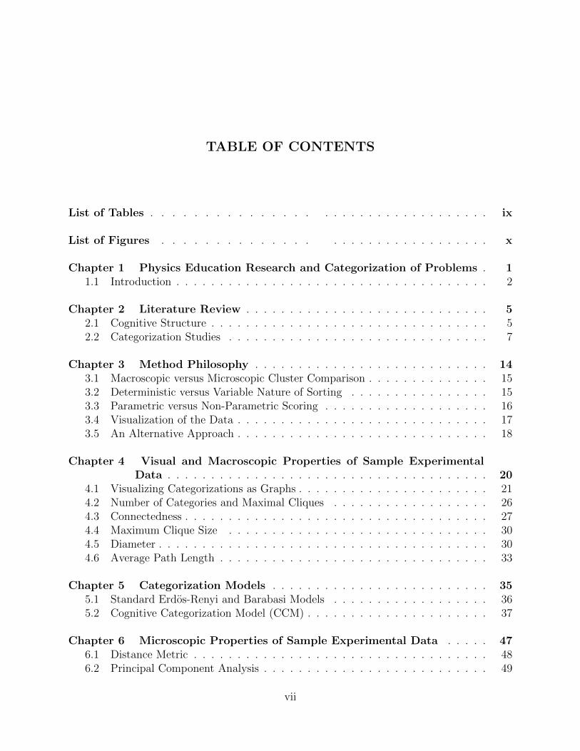
TABLE OF CONTENTS
List of Tables . . . . . . . . . . . . . . . . . . . . . . . . . . . . . . . . . . ix
List of Figures . . . . . . . . . . . . . . . . . . . . . . . . . . . . . . . . x
Chapter 1 Physics Education Research and Categorization of Problems . 11.1 Introduction . . . . . . . . . . . . . . . . . . . . . . . . . . . . . . . . . . . . 2
Chapter 2 Literature Review . . . . . . . . . . . . . . . . . . . . . . . . . . . . 52.1 Cognitive Structure . . . . . . . . . . . . . . . . . . . . . . . . . . . . . . . . 52.2 Categorization Studies . . . . . . . . . . . . . . . . . . . . . . . . . . . . . . 7
Chapter 3 Method Philosophy . . . . . . . . . . . . . . . . . . . . . . . . . . . 143.1 Macroscopic versus Microscopic Cluster Comparison . . . . . . . . . . . . . . 153.2 Deterministic versus Variable Nature of Sorting . . . . . . . . . . . . . . . . 153.3 Parametric versus Non-Parametric Scoring . . . . . . . . . . . . . . . . . . . 163.4 Visualization of the Data . . . . . . . . . . . . . . . . . . . . . . . . . . . . . 173.5 An Alternative Approach . . . . . . . . . . . . . . . . . . . . . . . . . . . . . 18
Chapter 4 Visual and Macroscopic Properties of Sample ExperimentalData . . . . . . . . . . . . . . . . . . . . . . . . . . . . . . . . . . . . . 20
4.1 Visualizing Categorizations as Graphs . . . . . . . . . . . . . . . . . . . . . . 214.2 Number of Categories and Maximal Cliques . . . . . . . . . . . . . . . . . . 264.3 Connectedness . . . . . . . . . . . . . . . . . . . . . . . . . . . . . . . . . . . 274.4 Maximum Clique Size . . . . . . . . . . . . . . . . . . . . . . . . . . . . . . 304.5 Diameter . . . . . . . . . . . . . . . . . . . . . . . . . . . . . . . . . . . . . . 304.6 Average Path Length . . . . . . . . . . . . . . . . . . . . . . . . . . . . . . . 33
Chapter 5 Categorization Models . . . . . . . . . . . . . . . . . . . . . . . . . 355.1 Standard Erdos-Renyi and Barabasi Models . . . . . . . . . . . . . . . . . . 365.2 Cognitive Categorization Model (CCM) . . . . . . . . . . . . . . . . . . . . . 37
Chapter 6 Microscopic Properties of Sample Experimental Data . . . . . 476.1 Distance Metric . . . . . . . . . . . . . . . . . . . . . . . . . . . . . . . . . . 486.2 Principal Component Analysis . . . . . . . . . . . . . . . . . . . . . . . . . . 49
vii
Chapter 7 Parameterizing Subsets . . . . . . . . . . . . . . . . . . . . . . . . 557.1 Experimental Parameters . . . . . . . . . . . . . . . . . . . . . . . . . . . . . 57
7.1.1 Problem Set Creation . . . . . . . . . . . . . . . . . . . . . . . . . . . 607.1.2 Expert-Novice Differentiation . . . . . . . . . . . . . . . . . . . . . . 60
Chapter 8 Subset Analysis: Data Mining the Categorization Graphs . . . 638.1 Monte Carlo analysis . . . . . . . . . . . . . . . . . . . . . . . . . . . . . . . 648.2 Simulated Annealing Analysis . . . . . . . . . . . . . . . . . . . . . . . . . . 65
Chapter 9 Conclusion . . . . . . . . . . . . . . . . . . . . . . . . . . . . . . . . 709.1 Outlook . . . . . . . . . . . . . . . . . . . . . . . . . . . . . . . . . . . . . . 73
APPENDICES . . . . . . . . . . . . . . . . . . . . . . . . . . . . . . . . . 76
Appendix A Categorization Model Pseudocode . . . . . . . . . . . . . . . . . 76A.1 Pseudocode . . . . . . . . . . . . . . . . . . . . . . . . . . . . . . . . . . . . 77
Appendix B Distance metric . . . . . . . . . . . . . . . . . . . . . . . . . . . . . 79B.1 Pseudocode . . . . . . . . . . . . . . . . . . . . . . . . . . . . . . . . . . . . 81
Appendix C Visualization technique . . . . . . . . . . . . . . . . . . . . . . . . . 82C.1 Pseudocode . . . . . . . . . . . . . . . . . . . . . . . . . . . . . . . . . . . . 82
Appendix D Problems in the Categorization Set . . . . . . . . . . . . . . . . . 84D.1 Prompt . . . . . . . . . . . . . . . . . . . . . . . . . . . . . . . . . . . . . . 84D.2 Problems . . . . . . . . . . . . . . . . . . . . . . . . . . . . . . . . . . . . . . 85
Appendix E Sorter Graphs . . . . . . . . . . . . . . . . . . . . . . . . . . . . . . 103
BIBLIOGRAPHY . . . . . . . . . . . . . . . . . . . . . . . . . . . . . . . . . . . . 146
viii
LIST OF TABLES
Table 2.1 Veldhuis’s Matrix Method. Deep Structures are listed along thetop. Surface Features are listed along the left. By “terms” Veldhuisincludes “physical arrangements of objects and literal physics terms”in the problem text.[3] Veldhuis created this set hoping that expertswould group the problems by column and novices would group theproblems by row. . . . . . . . . . . . . . . . . . . . . . . . . . . . . 10
Table 5.1 CCM Model Parameters . . . . . . . . . . . . . . . . . . . . . . 43
Table 7.1 Chapter titles Chapter titles taken from Walker’s textbook as arepresentative list. . . . . . . . . . . . . . . . . . . . . . . . . . . . 61
Table 7.2 TIPP levels A limited hierarchy of the cognitive processes describedby the TIPP. Most problems in a standard physics textbook require ahighest declarative knowledge process of Comprehension–Integrating,and procedural knowledge process of Retrieval–Executing [5]. Thelevel indicates the numeric value we scored the highest cognitive pro-cess required by each problem. . . . . . . . . . . . . . . . . . . . . 61
Table 8.1 Rigging parameters Variability explained by each of our problemvariable groups among our 10-problem subsets. From this we seethat the Chapter was an important variable, followed by the TIPP-Pstatistic. . . . . . . . . . . . . . . . . . . . . . . . . . . . . . . . . . 66
ix
LIST OF FIGURES
Figure 4.1 Simple example graph: When two problems are in the same cat-egory more than once (problems 1 and 9 as well as problems 3, 5,and 7 in this example) the edges drawn between those two corre-sponding vertices are thicker. The line width of each edge was takenproportional to the square of the number of connections between twovertices. . . . . . . . . . . . . . . . . . . . . . . . . . . . . . . . . . 24
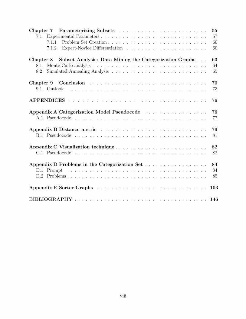
Figure 4.2 MSU physics study sorter graphs: Displayed from left to rightare the categorization graphs for representative sorters. Sorters 2and 16 were experts and sorters 20 and 30 were novices. Sorters 2and 30 did very little multiple categorization, sorter 20 did a goodbit of multiple categorization. Sorter 16 was unique in choosing tocategorize each problem between 2 and 3 times. Appendix E containsgraphs with each node labeled by the problem number for all sorters,including those shown here. . . . . . . . . . . . . . . . . . . . . . . 25
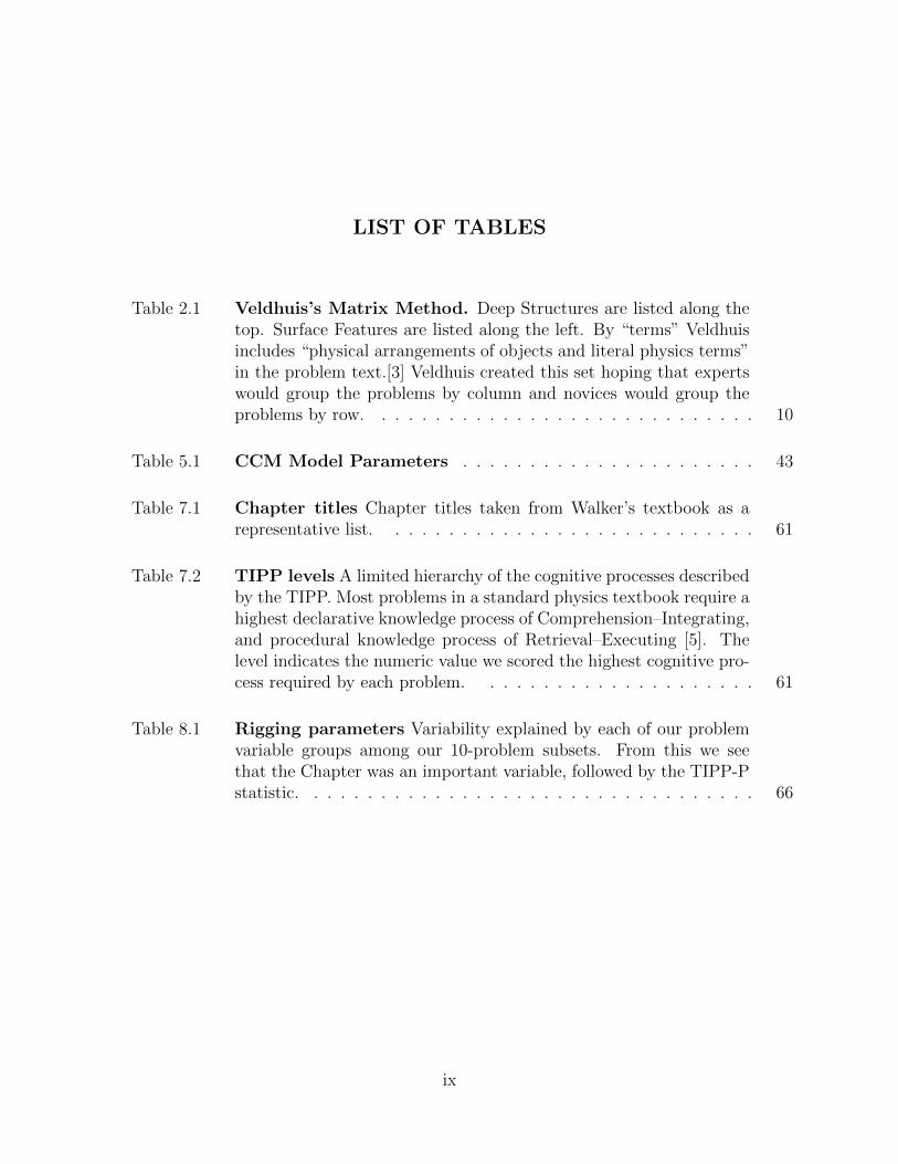
Figure 4.3 Distribution of Number of Categories: Here we see the ECDFsof the number of category distributions for experts and novices sep-arately. The faculty set is displayed using the dashed curve and thenovice set is displayed using the dotted curve. We also compare thesedistributions to a sample (N = 1000) shifted binomial distributionwith probability ρ = 0.204. A Kolmogorov–Smirnov test comparingthese two distributions suggests that expert and novice categoriza-tions are not distinguishable based on category number (p = 0.4793),and both are well approximated by the same shifted binomial distri-bution. . . . . . . . . . . . . . . . . . . . . . . . . . . . . . . . . . 28
Figure 4.4 Number of 3-cycles: This is the distribution of the number of 3-cycles for experts and novices. A Kolmogorov–Smirnov test suggeststhat experts and novices are not distinguishable based on their 3-cycledistributions (p = 0.1584). . . . . . . . . . . . . . . . . . . . . . . . 29
x
Figure 4.5 Maximum Clique Size: This is the distribution of the maximumclique size for experts and novices. A Kolmogorov–Smirnov test sug-gests that experts and novices are not distinguishable based on theirmaximum clique size distributions (p = 0.0587). . . . . . . . . . . . 31
Figure 4.6 Diameter: This is the distribution of the diameter of the expertsand novices. A Kolmogorov–Smirnov test suggests that experts andnovices are not distinguishable based on their diameter distributions(p = 0.6432). . . . . . . . . . . . . . . . . . . . . . . . . . . . . . . 32
Figure 4.7 Average Path Length: This is the distribution of the average pathlength for experts and novices. A Kolmogorov–Smirnov test suggeststhat experts and novices are not distinguishable based on their aver-age path length distributions (p = 0.3906). . . . . . . . . . . . . . . 34
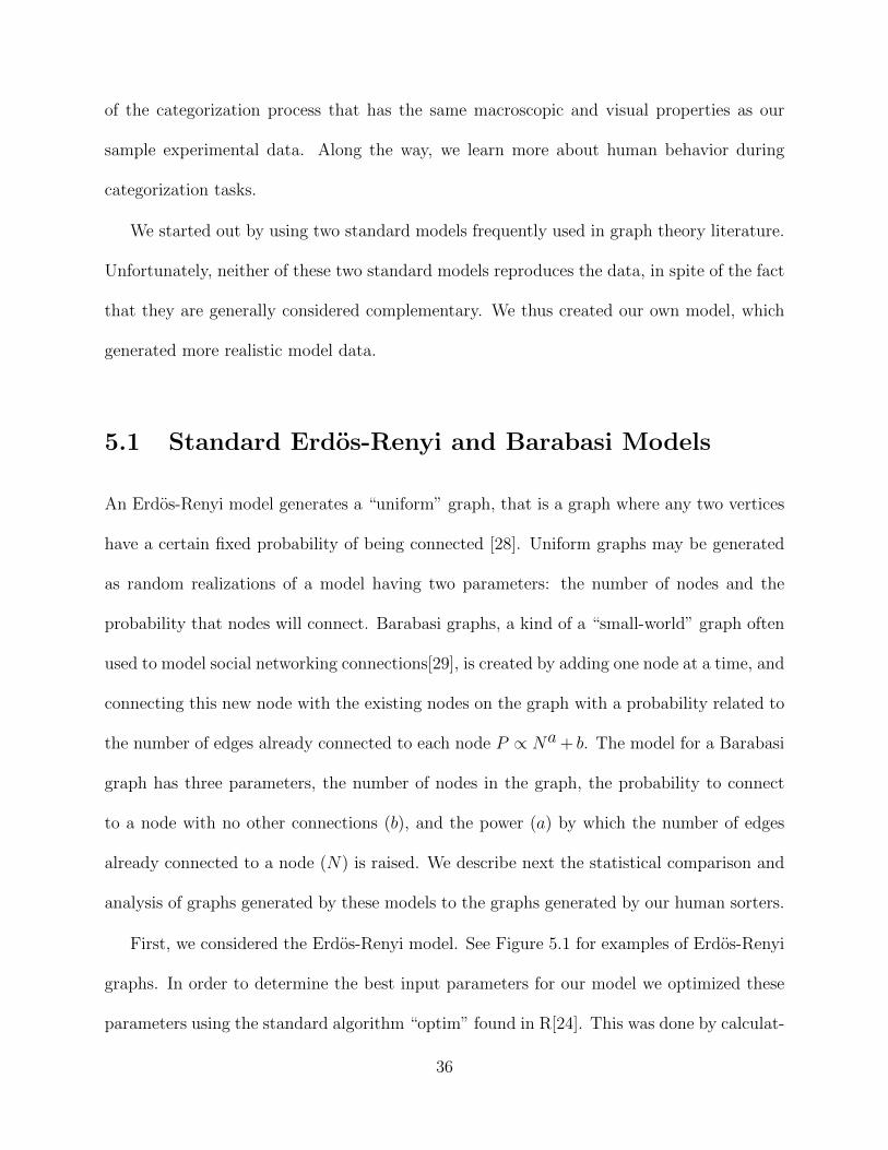
Figure 5.1 Erdos-Renyi and Barabasi graphs: The two graphs on the topare Erdos-Renyi graphs created using optimized parameters that bestfit the 3 cycle distributions of experts and novices. On the bottom,we see two Barabasi graphs. . . . . . . . . . . . . . . . . . . . . . . 38
Figure 5.2 3-cycle distributions Erdos-Renyi model: This is an ECDF ofthe 3-cycle distribution for sorters and the Erdos-Renyi model. Herethe dashed line corresponds to the Erdos-Renyi model while the solidline corresponds to the sorter data. . . . . . . . . . . . . . . . . . . 39
Figure 5.3 3-cycle distributions Barabasi model: This is an ECDF of the3-cycle distribution for the sorters and the Barabasi model. Here thedashed line corresponds to the Barabasi model while the solid linecorresponds to the sorter data. . . . . . . . . . . . . . . . . . . . . 40
Figure 5.4 3-cycle distributions Here we see the 3-cycle distributions for thedifferent CCMs. The model that fits the best is v3 (Equation 5.3),
where the multiple categorization probability is βC . . . . . . . . . 44
Figure 5.5 Representative CCM graphs: These are some representative graphsfor the CCM using optimized input parameters. Qualitatively theymatch up much better to the sorter graphs seen in Figure 4.2. . . . 46
xi
Figure 6.1 PCA of the sorter data: Here we see the PCA plot of the sorters.PC1 is the coordinate along the first principal axis, and PC2 is thecoordinate along the second principal axis. Sorter known by us to beexperts are marked by circles while sorters known by us to be novicesare marked by triangles. Each point is labeled on the left by the sorternumber. The second principal component discriminates experts fromnovices. . . . . . . . . . . . . . . . . . . . . . . . . . . . . . . . . . 53
Figure 6.2 Validating the use of PCA on the sorter data: This is a plot ofthe cumulative relative importance of each subsequent principal com-ponent. This shows that most of the variation is well-described by thefirst two principal components. Therefore using PCA for dimensionreduction is an appropriate choice for this data. . . . . . . . . . . . 54
Figure 7.1 Problem Dependence of PCA (Top) This is the PCA plot of thesorters for the entire set of problems from our previous study [6].
Both a Cramer’s test (p = 0.048) and a Hotelling’s test (p < 10−5)find the expert and novice groups to be distinct at a 95% confidencelevel. PC1 is the coordinate along the first principal axis, and PC2is the coordinate along the second principal axis. Sorters known byus to be experts are marked by circles while sorters known by usto be novices are marked by filled triangles. The second principalcomponent discriminates experts from novices. . . . . . . . . . . . 58
Figure 7.2 Problem Dependence of PCA This is the PCA plot of the sortersconsidering only the problems from Singh’s study. Both a Cramer’stest (p = 0.041) and a Hotelling’s test (p < 10−5) find the expertand novice groups to be distinct at a 95% confidence level. PC1 is thecoordinate along the first principal axis, and PC2 is the coordinatealong the second principal axis. Sorters known by us to be experts aremarked by circles while sorters known by us to be novices are markedby filled triangles. The second principal component discriminatesexperts from novices. . . . . . . . . . . . . . . . . . . . . . . . . . . 59
Figure 8.1 Rigging fraction This is a histogram of the rigging fraction for thesubsets with a random starting point. The shaded gray box indicatesthe rigging fraction of the Singh subset. From this, we can see thatthe Singh subset has more problems in common with its nearest localoptimum than does any of the random subsets studied. . . . . . . . 69
xii

Figure 9.1 The pillars of expert-novice differentiation. Here we see thekey parts of discriminating experts and novices on a categorizationtask. Deep structure (content), procedural knowledge (the kinds oftasks that a problem requires), and problem difficulty (easy questionstend to work better than hard questions). . . . . . . . . . . . . . . 72
Figure D.1 Diagram for problem 1. . . . . . . . . . . . . . . . . . . . . . . . . . 85
Figure D.2 Diagram for problem 4. . . . . . . . . . . . . . . . . . . . . . . . . . 86
Figure D.3 Diagram for problem 6. . . . . . . . . . . . . . . . . . . . . . . . . . 87
Figure D.4 Diagram for problem 8. . . . . . . . . . . . . . . . . . . . . . . . . . 88
Figure D.5 Diagram for problem 9. . . . . . . . . . . . . . . . . . . . . . . . . . 89
Figure D.6 Diagram for problem 13. . . . . . . . . . . . . . . . . . . . . . . . . 90
Figure D.7 Diagram for problem 14. . . . . . . . . . . . . . . . . . . . . . . . . 91
Figure D.8 Diagram for problem 17. . . . . . . . . . . . . . . . . . . . . . . . . 92
Figure D.9 Diagram for problem 18. . . . . . . . . . . . . . . . . . . . . . . . . 93
Figure D.10 Diagram for problem 19. . . . . . . . . . . . . . . . . . . . . . . . . 94
Figure D.11 Diagram for problem 27. . . . . . . . . . . . . . . . . . . . . . . . . 96
Figure D.12 Diagram for problem 28. . . . . . . . . . . . . . . . . . . . . . . . . 97
Figure D.13 Diagram for problem 30. . . . . . . . . . . . . . . . . . . . . . . . . 97
Figure D.14 Diagram for problem 34. . . . . . . . . . . . . . . . . . . . . . . . . 98
Figure D.15 Diagram for problem 47. . . . . . . . . . . . . . . . . . . . . . . . . 102
Figure E.1 The categorization graph of Sorter 1, an expert. . . . . . . . . . . . 104
Figure E.2 The categorization graph of Sorter 2, an expert. . . . . . . . . . . . 105
xiii

Figure E.3 The categorization graph of Sorter 3, an expert. . . . . . . . . . . . 106
Figure E.4 The categorization graph of Sorter 4, an expert. . . . . . . . . . . . 107
Figure E.5 The categorization graph of Sorter 5, an expert. . . . . . . . . . . . 108
Figure E.6 The categorization graph of Sorter 6, an expert. . . . . . . . . . . . 109
Figure E.7 The categorization graph of Sorter 7, an expert. . . . . . . . . . . . 110
Figure E.8 The categorization graph of Sorter 8, an expert. . . . . . . . . . . . 111
Figure E.9 The categorization graph of Sorter 9, an expert. . . . . . . . . . . . 112
Figure E.10 The categorization graph of Sorter 10, an expert. . . . . . . . . . . . 113
Figure E.11 The categorization graph of Sorter 11, an expert. . . . . . . . . . . . 114
Figure E.12 The categorization graph of Sorter 12, an expert. . . . . . . . . . . . 115
Figure E.13 The categorization graph of Sorter 13, an expert. . . . . . . . . . . . 116
Figure E.14 The categorization graph of Sorter 14, an expert. . . . . . . . . . . . 117
Figure E.15 The categorization graph of Sorter 15, an expert. . . . . . . . . . . . 118
Figure E.16 The categorization graph of Sorter 16, an expert. . . . . . . . . . . . 119
Figure E.17 The categorization graph of Sorter 17, an expert. . . . . . . . . . . . 120
Figure E.18 The categorization graph of Sorter 18, an expert. . . . . . . . . . . . 121
Figure E.19 The categorization graph of Sorter 19, a novice. . . . . . . . . . . . 122
Figure E.20 The categorization graph of Sorter 20, a novice. . . . . . . . . . . . 123
Figure E.21 The categorization graph of Sorter 21, a novice. . . . . . . . . . . . 124
Figure E.22 The categorization graph of Sorter 22, a novice. . . . . . . . . . . . 125
xiv
Figure E.23 The categorization graph of Sorter 23, a novice. . . . . . . . . . . . 126
Figure E.24 The categorization graph of Sorter 24, a novice. . . . . . . . . . . . 127
Figure E.25 The categorization graph of Sorter 25, a novice. . . . . . . . . . . . 128
Figure E.26 The categorization graph of Sorter 26, a novice. . . . . . . . . . . . 129
Figure E.27 The categorization graph of Sorter 27, a novice. . . . . . . . . . . . 130
Figure E.28 The categorization graph of Sorter 28, a novice. . . . . . . . . . . . 131
Figure E.29 The categorization graph of Sorter 29, a novice. . . . . . . . . . . . 132
Figure E.30 The categorization graph of Sorter 30, a novice. . . . . . . . . . . . 133
Figure E.31 The categorization graph of Sorter 31, a novice. . . . . . . . . . . . 134
Figure E.32 The categorization graph of Sorter 32, a novice. . . . . . . . . . . . 135
Figure E.33 The categorization graph of Sorter 33, a novice. . . . . . . . . . . . 136
Figure E.34 The categorization graph of Sorter 34, a novice. . . . . . . . . . . . 137
Figure E.35 The categorization graph of Sorter 35, a novice. . . . . . . . . . . . 138
Figure E.36 The categorization graph of Sorter 36, a novice. . . . . . . . . . . . 139
Figure E.37 The categorization graph of Sorter 37, a novice. . . . . . . . . . . . 140
Figure E.38 The categorization graph of Sorter 38, a novice. . . . . . . . . . . . 141
Figure E.39 The categorization graph of Sorter 39, a novice. . . . . . . . . . . . 142
Figure E.40 The categorization graph of Sorter 40, a novice. . . . . . . . . . . . 143
Figure E.41 The categorization graph of Sorter 41, a novice. . . . . . . . . . . . 144
xv

Chapter 1
Physics Education Research and
Categorization of Problems
Physicists oftentimes pride themselves on being resourceful problem solvers. Larkin et al.
concluded that the basis of this problem solving ability is the array of cognitive connections
between multiple concepts, making each physics concept a part of a coherent whole rather
than disparate bits of information [8]. Fuller points out the importance of a good conceptual
understanding when he says, “Every physicist knows the importance of having the correct
concept in mind before beginning to solve a problem” [9, emphasis mine].
Categorization studies comparing experts and novices started with Chi et al., who stud-
ied the categorization of introductory physics problems [1]. This study, to date, has been
cited over 3000 times. It has been critical in the study of the differences between experts
and novices in many areas, such as Clinical Psychology [10], dinosaur expertise [11], wine
tasting [12], and even Star Wars philosophy [13]. All of these studies go back to the same ap-
parently straightforward result in physics: novices categorize introductory physics problems
1

by “surface features” (e.g. “incline,” “pendulum,” or “projectile motion”), while experts
use “deep structure” (e.g. “energy conservation” or “Newton’s second law”).
Our understanding of expertise was established by the seminal study done by Chi et al. [1].
However, replicating this experiment has been challenging. More often than not, attempts
to verify it fail, as an informal survey among physics education researchers indicated. This
is a puzzling fact given the sensibility and popularity of the result of Chi et al.. It has
not been until more recently that the physics education research community has begun to
understand why this might be while it has been grappling with different understandings
of student learning and the conceptualization of expertise [14]. The earlier view held that
students strongly hold misconceptions which must be defeated by instruction [14]. This
view was limited in explaining how students actually acquire expertise. However, more
recently, the view of student learning has become more nuanced [15, 14]. Instead, students
have many intuitive resources that they may apply to solving the problems that they face.
As students learn, they also learn the productive resources which may be applied to the
problems that they face which will lead to positive outcomes. The paradigm shift about the
understandings of student learning leads us to reconsider the paradigm that the community
has used to understand expertise.
1.1 Introduction
In order to re-examine this understanding, we have designed and carried out a categorization
experiment and developed a novel methodology to analyze that experiment [6]. Chapter of
this thesis will discuss the developments in our understanding of student learning as well as
review categorization studies in physics over the past 31 years. This discussion will include
2

a summary of the different analysis methods used by each of the research groups, and allow
us to understand the advantages and disadvantages of each method.
Chapter will compare and contrast the previous analysis methods used to analyze cat-
egorizations. Given the aforementioned difficulties in replicating the seminal experiment of
Chi et al. and the revolution in understanding of learning, we will critique these methods
based on three properties. These are that an analysis method should be problem specific,
objective, and robust against outliers. With these requirements in mind, we will motivate
the need for the method we have developed to fulfill these requirements.
Chapter will introduce the key idea supporting this new method that we have created
to describe categorization data. The first step is to convert an individual sorter’s catego-
rization into a graph network. Expert and novice sorters’ graphs are then compared based
on the macroscopic properties of these graphs. We find that the key factor discriminating
sorters is not expertise, instead it is their sorting behavior, something we term “stacking”
vs. “spreading.”
Chapter will develop a statistical model which will seek to find the common pattern be-
hind this macroscopic comparison. In creating this model we choose only a three parameters
to describe the group behavior: The number of questions sorted (a parameter fixed by the
experiment), the average number of categories, and the multiple categorization parameter.
As is customary in categorization experiments, a single problem may be placed into more
than one category, and the multiple categorization parameter describes the probability that
multiple categorization occurs. Due to the fact that the individual multiple categorization
probability decreases with the individual number of categories created, this reinforces the
“stacker” vs. “spreader” interpretation.
3
Chapter will detail how to compare any two categorization graphs to each other using a
distance metric we developed and will visualize the relative position of sorters using Principal
Components Analysis (PCA) [6]. This visualization technique also confirms the “stacking”
and “spreading” behavior observed as the largest source of variation in our categorization
experiment. However, the second largest source of variation found by the PCA is due to
expertise. This finding suggests that the experiment of Chi et al. has been difficult to
replicate because the largest source of variation was not due to expertise. We explore next
why a particular set of problems would discriminate experts from novices, while others do
not, by considering many subsets of the large problem set categorized by the sorters.
In Chapter we will discuss the different statistics used to describe the problem sets.
These include the cognitive and contextual features of the problems as well as the ability
that a subset has to discriminate expert and novice sorters. The contextual features of
the problems include a problem’s chapter and difficulty. The discriminatory properties of
subsets are found by using both parametric and non-parametric tests which compare the
PCA coordinates of the expert and novice groups.
Finally, in Chapter , we will discuss the results of this subset analysis and determine
which properties are important in discriminating experts from novices in a categorization
experiment. We will discuss the importance, not only of problem content, but requiring
sorters to categorize problems which require diverse solution types.
4
Chapter 2
Literature Review
2.1 Cognitive Structure
Before we begin discussing categorization studies, we should define what an expert is from
a cognitive perspective. We know that we may identify an expert by his skill set, however,
using a skill set to define an expert is a rather circular definition, so we will do better.
Larkin et al. [8] consider the research on experts in several fields—namely Chess, algebra,
and physics—to help us arrive at an answer. Cognitive research has taught us how experts
store knowledge and about an expert’s ability to access that knowledge. From a cognitive
viewpoint, an expert’s knowledge of introductory topics may be thought of as a well indexed,
easy to access database. Moreover, this database is also well cross-referenced so that the
main topics are also easily connected. The difference can be seen in this anecdote regarding
Chess experts and novices. If a chess expert is shown a position from an actual match with
about 25 pieces on the board and allowed to study it for 5–10 seconds, he will be able to
reproduce it with about 90% accuracy, while a novice will typically be able to replace only
5

about 20–25% of the pieces [8]. This stark difference is due in large part to a memory
phenomena called “chunking.”[8] Cognitive research has shown that people can only hold
relatively few “objects” in short term memory. Chess experts will quickly recognize a familiar
pawn structure and placement of key pieces; the difference is therefore easily explained since a
chess expert memorizes structures while the novices attempts to remember a position piece
by piece. However, people studying chess experts have found out how to “rig the game”
so that expert performance reverts back to novice ability. They can do this by putting a
position on the board that is purely random which could never happen in a real game. For
example, never will a pawn be in the first rank nor the white king adjacent to the black
king. Positions like these have none of the familiar chunks that an expert chess player will
recognize, therefore the performance on this task will be the same for experts and novices.
In order to compare expert and novice cognitive structures, we need to define our under-
standing of the underlying process of categorization. Different understandings of the under-
lying process of categorization will lead to different statistical analysis methods. Chi et al.
seem to view categorization as a deterministic process, as evidenced by the “double-check”
step in their experimental method. They see any minor replication variation as evidence of
an underlying method. On the other hand, one of the phenomena that physics education
research has to grapple with is the variability of learner responses to what appear to be
identical scenarios, see for example Scherr [16] dealing with problems in relativity and Frank
et al. [17] dealing with problems in motion. Rather than interpreting card-sorting outcomes
as reflections of stable theories or beliefs, an alternative model is that they are based on ad
hoc assemblies of more simple intuitions (similar to “phenomenological primitives,” [15] or
“resources” [14]) — those are then assembled “on-the-fly,” and the particular assembly may
6
vary depending on circumstances. There is no reason to expect that card-sorting experiments
are immune to this variability, and one may thus expect that any sorter who categorizes the
same set of problems on separate occasions would return different results, although he or she
might even recognize the problems that are used. We cannot control the actual mechanisms
potentially underlying these “random” outcomes, but have accounted for the resulting vari-
ability in the choice of our statistical methods. In addition, we use sample-based statistics
to interpret our categorization data, realizing that our sample is only part of a vastly larger
population.
2.2 Categorization Studies
The novice group of Chi et al.’s study was made up of eight students who had just finished
the first semester of an introductory university physics class, and the expert group was made
up of eight advanced Ph.D. physics students. Both groups were given the instructions to
sort the problems “based on similarity of solution”[1]. Problems were allowed to be placed
in two (or more) categories if the sorter so desired; we call this “multiple categorization,” as
opposed to “single categorization,” where each problem would have to be sorted in one and
only one category.
Each sorter categorized their set in front of a member of the research team according to
a uniform protocol. Sorters were required to sort the problems without paper and pencil
to prevent them from actually solving the problems. After sorting the problems a second
time — to check for consistency — the sorters explained the reasoning for their groupings.
After a qualitative analysis of the category names used by more than two sorters, Chi et al.’s
group concluded that the key distinction between experts and novices is, quite sensibly, that
7

experts sort problems based on the physics principle required to solve each problem, while
novices sort the problems based on surface features. This difference in categorization, Chi
et al. concluded, was an experts’ ability to convert contextual cues from the problem texts
and figures into the physics principles that are required to solve those problems. The main
message from Chi’s paper is that this difference in categorization behavior allows experts to
be better problem solvers than novices [1].
In order to reevaluate these conclusions de Jong and Ferguson-Hessler studied both expert
and novice categorizations of “elements of knowledge” required in a typical Electricity and
Magnetism course [18]. In this study, the novice group consisted of 47 first-year students who
had just finished the Electricity and Magnetism course, and the expert group consisted of four
staff members, each of whom had taught the course for multiple years [18]. The “elements of
knowledge” categorized were simply bits of information and ideas needed to solve 12 “classic”
E&M problems. For example, in order to find the electric field due to a semi-infinite line of
charge with a constant charge per unit length using Coulomb’s law one needs four “elements
of knowledge.” First, a person would need to understand the physical meaning of a semi-
infinite line of charge. Second, a person would need to know the mathematical definition of
Coulomb’s law. Third, a person would need to know the principle of superposition and that
an application of this principle would be to take the integral of a vector quantity. Fourth, a
person would need to know the relationship between electric force and electric field (de Jong
and Ferguson-Hessler defined Coulomb’s law for the force only and not the electric field).
A total of 65 “elements of knowledge” were placed on individual cards and given to the
participants in a random order. The participants were asked to sort the cards into piles and
give names to their piles, indicating which, if any, elements were unfamiliar by putting them
8

in a separate pile. de Jong and Ferguson-Hessler found that novices who performed well
in the class generally sorted the “elements of knowledge” into groups according to the each
classic problem which generated that group. However, the experts’ advanced knowledge had
been re-organized in a “hierarchical way” useful for upper-level physics applications rather
than in the manner of the good novice problem solvers. That is, these elements tended to
be organized according to principles (Coulomb’s law, Biot-Savart,. . . ) and processes rather
than in groups useful for solving “classic” problems.
In a subsequent study, Veldhuis attempted to verify the result of Chi et al. [2]. Veld-
huis had three groups, a novice group comprised of 94 introductory physics students, an
intermediate group of 5 students who had just finished classical mechanics, and an expert
group of 20 physics professors—among whom only 2 had not taught calculus-based physics.
Veldhuis created four different categorization sets, one of which was given to each subject to
categorize according to a protocol similar to that used by Chi et al.’s group. The first set was
created in an attempt to mimic the Chi et al. problem set [3], and the second was a control
set with a similar collection of end-of-chapter problems. In contrast, the third and fourth
sets were carefully constructed so that each problem had only a single physics principle and
a single surface feature from a set of principles and surface features [2]. For example, Table
2.1 shows how the third set was constructed by populating a matrix of four surface and four
conceptual features. The fourth set was also “rigged.” It had the same number of cards,
but only two surface and two conceptual features. Veldhuis could not draw a conclusion
from the categorizations from his first two problem sets. However, sets 3 and 4 agreed with
Chi et al. in that experts categorize problems based on physics principles while novices show
a “more complex behavior.” [2, 3] Ironically, Veldhuis observed that distinguishing experts
9

Table 2.1: Veldhuis’s Matrix Method. Deep Structures are listed along the top. SurfaceFeatures are listed along the left. By “terms” Veldhuis includes “physical arrangements ofobjects and literal physics terms” in the problem text.[3] Veldhuis created this set hopingthat experts would group the problems by column and novices would group the problems byrow.
Newton II1 E cons2 ~p cons3 ~L cons4
Spring Prob 16 Prob 2 Prob 4 Prob 9Ramp Prob 11 Prob 6 Prob 12 Prob 15Pulley Prob 5 Prob 14 Prob 13 Prob 8Terms Prob 3 Prob 10 Prob 7 Prob 1
and novices based on surface features of their categorizations failed unless the desired physics
features — conceptual and surface — were built into the design of the experiment.
More recently, the work done in Singh’s group at the University of Pittsburgh has broad-
ened the application of “card-sorting” to other fields [19, 20, 7, 21]. Mason and Singh
compared students in introductory physics courses with both physics graduate students and
physics faculty. Mason and Singh created two categorization sets of twenty-four problems
each. The first set was created in an attempt to mimic Chi et al.’s set. Seven problems
were directly from Chi et al.’s original set, based on examples given in the paper, while the
remainder of the Chi et al.’s original set is apparently lost in history. A second set was
devised because the results from the first set showed “major differences” with Chi et al.’s
data [19, 20], which may not be surprising given Veldhuis’s previous results [2, 3]. Each
subject, upon reading the problems, filled in three columns on a response sheet: category
name, the appropriateness of the category name, and the identity of problems that fit in
the category. Mason and Singh then rated each problem’s category as “good,” “moderate,”
or “poor” based on each sorter’s description of the category. A category was considered
“good” if it was based on the underlying physics principles. Finally, the authors asked a
10
faculty panel to validate their ratings by following the same procedure on a subset of the
categorizations.
Mason and Singh found that the problems taken directly from Chi et al.’s original study
were placed by novices in “good” categories far less often than they did on average, deter-
mining that they were generally from topics more difficult to novice students. For example,
difficult topics for novices might have been rotational motion, non-equilibrium applications
of Newton’s 2nd law, or the Work-Energy theorem [19, 20]. Mason and Singh also found that
the superficial category names were far less prevalent in their study than in Chi’s original
study. It is possible that the shift away from novices’ use of superficial category names is
due to a change in curricular focus precipitated by Chi et al.’s result. Contrary to the sharp
distinction found by Chi et al., Mason and Singh found that there was some overlap between
the calculus-based introductory physics students and the graduate students [19, 20].
In a follow-up study, Singh [7] asked graduate student teaching assistants to perform a
similar categorization exercise, both as themselves and through the eyes of their students, and
compared both types of their categorizations to physics faculty and introductory students. In
contrast with Chi et al., Singh considered the physics faculty as the “true experts” and only
looked at graduate students as a sort of intermediate group. Similar to Mason and Singh,
problem categories were rated to be “good”, “moderate,” or “poor,” validated by a faculty
panel. Singh found that the graduate students acting as introductory students performed
better on the categorization task than did actual introductory students, thus overestimating
their students [7]. Singh found that the professors performed best on the categorization
task, distinguishing this group from the categorizations of the graduate students acting as
themselves. This suggested that the use of graduate students as an expert group is not
11
entirely accurate, as their behavior is not truly expert-like.
Finally, in a separate study, Lin and Singh also carried out a categorization study con-
cerning Quantum Mechanics problems [21]. For this task the novice group consisted of
twenty-two Junior and Senior physics majors taking Quantum Mechanics. The expert group
consisted of six faculty members [21]. In contrast to the previous studies mentioned here,
Lin and Singh chose to have a three-member faculty panel evaluate all of the categorizations,
scoring each category as either good, moderate, or poor. In contrast to the studies of intro-
ductory physics problems, in Lin and Singh’s study, the expert group had more variability,
as even the faculty panel did not see this task in stark terms. Two of the panel members
even said that they disliked using the terms “good” and “poor” to describe a categorization
of Quantum Mechanics problems; this reservation was not voiced by the raters in the intro-
ductory problem categorization studies [21]. Similarly, the faculty panel members said that
sometimes they preferred another categorization choice to their own [21]. All of this, Lin
and Singh conclude, was due to the more difficult nature of the problems. In any case, it is
clear that no “ideal” set of groupings existed, and it was impossible to simply assign some
“score” to a given categorization.
As you can see, interest in replicating the result of Chi et al. has increased in the past
decade, possibly due to the fact that the PER community has come to change its under-
standing of learning. This renewed interest has led to correspondence with the lead author,
Chi. Anyone interested in replicating Chi et al.’s experiment would want two things from
the original study: The problems used and the analysis method used. However, in corre-
spondence with Mason and Singh, Chi states that all but a few problems from the original
study “had been discarded and were not available” [20]. Furthermore, the exact analysis
12
method Chi et al. used is apparently lost to history as well [22]. From these communications
as well as the description of the analysis method from the original paper, it is apparent that
Chi et al. did not use all of the problems in their analysis. The truth is simply that so much
of the information from Chi et al.’s original study has been lost that we cannot falsify or
verify it.
In summary, replicating Chi et al.’s seminal experiment is challenging. More often than
not, attempts to repeat it fail, as an informal survey among physics education researchers
indicates — however, such null-results do not get published. Yet, as a community of physics
educators, we hold a firm belief that deep down there is a significant difference in problem
solving behavior between experts and novices, and that categorization is an important piece
of the puzzle. Quantifying this difference, however, more often than not, remains elusive.
13
Chapter 3
Method Philosophy
This chapter will compare and contrast the previous analysis methods used to analyze cat-
egorizations. Given the aforementioned difficulties in replicating the seminal experiment of
Chi et al. and the revolution in understanding of learning, we will critique these methods
based on three properties. These are that an analysis method should be problem specific,
objective, and robust against outliers. With these requirements in mind, we will motivate
the need for the method we have developed to fulfill these requirements.
While Chi et al.’s method has been the predominant paradigm for follow-up studies, their
methodology is based on a certain model of the categorization process. Using a different
model, one will arrive at a different methodology. Given the importance of this experimen-
tal technique, we believe it is important to understand the underlying model and consider
alternatives to its assumptions.
14

3.1 Macroscopic versus Microscopic Cluster Compari-
son
Chi et al.’s group looked at a processed version of the category names agreed upon by
multiple sorters and counted the number of problems in each category name [1]. Their
analysis does not seem to hinge on the identity of the problems in each group, merely the
number of problems in that group. For example, if two sorters both used the category name
“Conservation of Energy” but one sorter put problems {1, 3, 5, 7, 9} in that set and the other
sorter put problems {2, 4, 7, 8, 9} in that set, Chi et al.’s analysis would count that as two
people who both used an energy related variant as a category and both had five problems in
that set. In other words, the sets would be treated identically. We argue that it is important
that these two groups should be treated differently, as they have few identical elements. We
believe that instead of just these “macroscopic” measures (sizes and names of groups), the
sorting results should also be compared on the “microscopic” level of individual problems.
3.2 Deterministic versus Variable Nature of Sorting
Different understandings of the underlying process of categorization will lead to different
statistical analysis methods. Chi et al. seem to view categorization as a deterministic pro-
cess, as evidenced by the “double-check” step in their experimental method. They see any
minor replication variation as evidence of an underlying method. That is, variation on the
second time through the cards is a chance to correct a mistake. On the other hand, one
of the phenomena that physics education research has to grapple with is the variability of
learner responses to what appear to be identical scenarios, see for example Frank et al. [17].
15

Rather than interpreting card-sorting outcomes as reflections of stable theories or beliefs,
an alternative model is that they are based on ad hoc assemblies of more simple intuitions
(similar to “phenomenological primitives,” [15] or “resources” [14]) — those are then as-
sembled “on-the-fly,” and the particular assembly may depend on circumstances which are
dynamic. There is no reason to expect that card-sorting experiments are immune to this
variability, and one may thus expect that any sorter who categorizes the same set of prob-
lems on separate occasions would return different results, although he or she might even
recognize the problems that are used. To wit, replication variation is expected. We cannot
control the actual mechanisms potentially underlying these “random” outcomes, but have
accounted for the resulting variability in the choice of our statistical methods. In addition,
we use sample-based statistics to interpret our categorization data, realizing that our sample
is only part of a vastly larger population.
3.3 Parametric versus Non-Parametric Scoring
Previous analysis methods [19, 20, 7, 21] describe each categorization individually with a
score, which is either a comparison to an “ideal” categorization set or an individual “grade” of
each set. These methods measure performance on the categorization task, where the scoring
criteria is an input of the evaluation process — the process starts with assumptions of what
properties an expert categorization will have. It may, however, not be clear what an “ideal”
set is, which in turn makes the scoring somewhat ambiguous. First, curricular emphasis
within any physics program varies over time; as does the researcher’s personal categorization.
Therefore that researcher may rate the same data differently if he or she were to re-evaluate
the same categorization set again. Second, the experiment will not be repeatable from
16
one group to another using these methods because each individual experimenter’s ideal
categorization of the same set will be different, possibly creating a large distortion in the
analysis. Third, as Lin and Singh found, as topics become more complex, an expert will
express uncertainty in his or her own choice, sometimes preferring the choice of another
to his or her own. Finally, if one evaluates each categorization subjectively based on the
expected deep structure category for each problem, one assumes the deep structure versus
surface features distinction rather than letting that be a conclusion of the statistical analysis.
We believe that any groupings should emerge from the data itself. In other words, the
properties and patterns of what makes a categorization expert-like should be an output of
the experiment. Similar to outcomes from non-parametric data-mining, it may not always be
clear what these characteristics mean, as they are frequently combinations of many features
or latent factors.
3.4 Visualization of the Data
Finally, several studies utilized dendograms to interpret their data, e.g., Veldhuis [2]. While
dendograms are intuitive, they are not very stable. Milligan [23] investigated a number of
clustering algorithms and compared them using Monte-Carlo generated data from a defined,
yet synthetic, cluster model which employed random perturbations. According to Milligan,
complete linkage clustering, a type of dendogram analysis, struggles to recover clusters when
there are outliers present in the dataset. Another type of dendogram analysis, single linkage
clustering, is highly sensitive to noise in the dataset. It is for these reasons that it is important
to pre-process any data, for example by removing outliers from the data set, in order to get a
dendogram that is clear and interpretable. Interpreting a dendogram is a subjective exercise
17

as each dendogram will have a unique threshold where the tree has clustered into groups, yet
has not begun to coalesce into a single stem on the tree. Some dendograms do not have any
distinguishable groups at all. We desired to have an experimental method that required no
pre-processing, with a reliable and easily interpretable output suitable for further analysis.
As a result, we have chosen a different approach, based on graphs.
3.5 An Alternative Approach
Given the above concerns, we explored a different model of analyzing and interpreting card-
sorting data. To describe clustering on an individual problem level, we decided to approach
the analysis as a network. Instead of looking at piles, we decided to look at individual
question cards (nodes in the network) and relationships (edges, in this case due to nodes
“being in the same pile”). Networks are well described by graph theory. As the relationship
“being in the same pile” has no direction (if problem A is in the same pile as B, then B is
in the same pile as A), we are looking at undirected graphs. The resulting graphs have the
advantage of converting an abstract network into an object that can both be visualized and
analyzed using an established canon of mathematical methods.
As scientists, we prefer simple explanations to complex ones, and sought to distinguish
experts from novices using the simplest test possible. It is for this reason that we compare
these categorizations’ macroscopic features before continuing on to microscopic features. The
key distinction between the macroscopic and microscopic scales is that the macroscopic scale
should not be sensitive to the identity of the problems, while the microscopic scale should be
highly sensitive to problem identity. In choosing mathematical methods for further analysis,
we were unexpectedly limited by one feature of Chi et al.’s and subsequent studies: the
18

“multiple categorization,” i.e., the fact that one and the same question card is allowed to be
in more than one pile. This presented a challenge to several existing algorithms. The key
measurement we make is a “distance” measurement between each pair of categorizations.
Given these distances, we used Principal Components Analysis (PCA) to visualize the data
in a few simple plots.
19

Chapter 4
Visual and Macroscopic Properties of
Sample Experimental Data
This chapter introduces the key idea supporting this new method that we have created to
describe categorization data. The first step is to convert an individual sorter’s categoriza-
tion into a graph network. Expert and novice sorters’ graphs are then compared based
on the macroscopic properties of these graphs. We find that the key factor discriminating
sorters is not expertise, instead it is their sorting behavior, something we term “stacking”
vs. “spreading.”
In order to cognitive structures of physics concepts, we designed and carried out a card-
sorting experiment on physics experts and novices at Michigan State University. A total
of 18 physics professors and 23 novices participated in our study. All of the novices had
completed at least the first semester of an introductory physics course at MSU. We gave
each sorter a set of 50 problems to sort based on similarity of solution. The physics faculty
were given the set and allowed to choose a time when they would complete the task at
20
their convenience while the novices were asked to complete the task during a window of a
few hours in an informally supervised setting. Each sorter categorized his or her problems
and recorded his groups and group names in a separate packet. Multiple categorization was
allowed, but it was in no way communicated to the individual sorters that this practice was
expected or endorsed. While this may be problematic if some sorters did not assume that
multiple categorization was allowed, it is the standard protocol for these sorts of experiments
[1, 7, 20].
4.1 Visualizing Categorizations as Graphs
Analyzing the experimental data in terms of graphs requires a shift in conceptualization.
As a simple example, consider ten questions categorized into four categories. Suppose that
the first category is Newton’s second law and contains problems {2, 4, 6, 8, 10}. Suppose
also that the second category is conservation of energy and contains problems {1, 3, 5, 7, 9},
the third category is conservation of momentum and contains problems {2, 3, 5, 7}, and the
fourth category is kinematics and contains problems {1, 4, 9}. At this stage in the process,
the names of the categories are irrelevant. In order to create a graph of categorization data
we represented questions (cards) as the nodes and used each category to create a set of edges.
To start out, we summarize the categorization information in a matrix T . This matrix is a
Boolean (0 |1) table with the items being sorted placed along the rows and the categories in
21
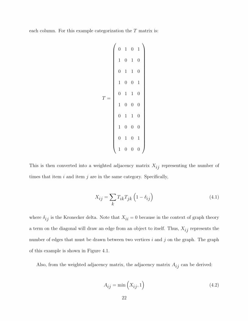
each column. For this example categorization the T matrix is:
T =
0 1 0 1
1 0 1 0
0 1 1 0
1 0 0 1
0 1 1 0
1 0 0 0
0 1 1 0
1 0 0 0
0 1 0 1
1 0 0 0
This is then converted into a weighted adjacency matrix Xij representing the number of
times that item i and item j are in the same category. Specifically,
Xij =∑k
TikTjk
(1− δij
)(4.1)
where δij is the Kronecker delta. Note that Xii = 0 because in the context of graph theory
a term on the diagonal will draw an edge from an object to itself. Thus, Xij represents the
number of edges that must be drawn between two vertices i and j on the graph. The graph
of this example is shown in Figure 4.1.
Also, from the weighted adjacency matrix, the adjacency matrix Aij can be derived:
Aij = min(Xij, 1
)(4.2)
22
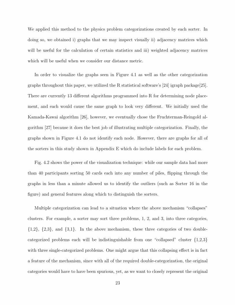
We applied this method to the physics problem categorizations created by each sorter. In
doing so, we obtained i) graphs that we may inspect visually ii) adjacency matrices which
will be useful for the calculation of certain statistics and iii) weighted adjacency matrices
which will be useful when we consider our distance metric.
In order to visualize the graphs seen in Figure 4.1 as well as the other categorization
graphs throughout this paper, we utilized the R statistical software’s [24] igraph package[25].
There are currently 13 different algorithms programmed into R for determining node place-
ment, and each would cause the same graph to look very different. We initially used the
Kamada-Kawai algorithm [26], however, we eventually chose the Fruchterman-Reingold al-
gorithm [27] because it does the best job of illustrating multiple categorization. Finally, the
graphs shown in Figure 4.1 do not identify each node. However, there are graphs for all of
the sorters in this study shown in Appendix E which do include labels for each problem.
Fig. 4.2 shows the power of the visualization technique: while our sample data had more
than 40 participants sorting 50 cards each into any number of piles, flipping through the
graphs in less than a minute allowed us to identify the outliers (such as Sorter 16 in the
figure) and general features along which to distinguish the sorters.
Multiple categorization can lead to a situation where the above mechanism “collapses”
clusters. For example, a sorter may sort three problems, 1, 2, and 3, into three categories,
{1,2}, {2,3}, and {3,1}. In the above mechanism, these three categories of two double-
categorized problems each will be indistinguishable from one “collapsed” cluster {1,2,3}
with three single-categorized problems. One might argue that this collapsing effect is in fact
a feature of the mechanism, since with all of the required double-categorization, the original
categories would have to have been spurious, yet, as we want to closely represent the original
23

12
3
4
5
6
7
8
910
Figure 4.1: Simple example graph: When two problems are in the same category morethan once (problems 1 and 9 as well as problems 3, 5, and 7 in this example) the edges drawnbetween those two corresponding vertices are thicker. The line width of each edge was takenproportional to the square of the number of connections between two vertices.
24

Sorter 2 Sorter 16
●
●
●
●
●
●
●
●
●
●
●●
●
●
●●
●
●●
●
●
●
●
●
●
●
●
●
●
●
●
●
●
●
●
●
●
●●
●
●
●
●
●
●
●
●
●
●
●
●
●
● ●
●
●
●
●
●
●●
●●
●●
●
●
●●
●
●
●
●
●
●
●
●
●
●
●
●
●●
●
●
●
●
●
●
●
●
●
●
●
●●
●
●
●
●
Sorter 20 Sorter 30
●
●
●
●
●
●
●
●●
●
●●
●
●
●
●●●
●
●
●
●
●
●
●●
●
●
●
●
●
●●
●
●●
●●
●
●
●
●
●
●
●
●
●
●●
●
●
●
●●
●
●
●
●●
●
●
●
●
●
●
●
●
●
●
●
●
● ●
●
●●●
●
●
●
●●
●
●
●●
●
●
●
●
● ●
●
●
●
●
●
●
●
●
Figure 4.2: MSU physics study sorter graphs: Displayed from left to right are thecategorization graphs for representative sorters. Sorters 2 and 16 were experts and sorters20 and 30 were novices. Sorters 2 and 30 did very little multiple categorization, sorter 20 dida good bit of multiple categorization. Sorter 16 was unique in choosing to categorize eachproblem between 2 and 3 times. Appendix E contains graphs with each node labeled by theproblem number for all sorters, including those shown here.
25

sorting, we need to be on the lookout for a possible loss of information upon converting each
sorting into a graph. We will do this by comparing the number of categories to an analogous
statistic from graph theory, the number of maximal cliques.
4.2 Number of Categories and Maximal Cliques
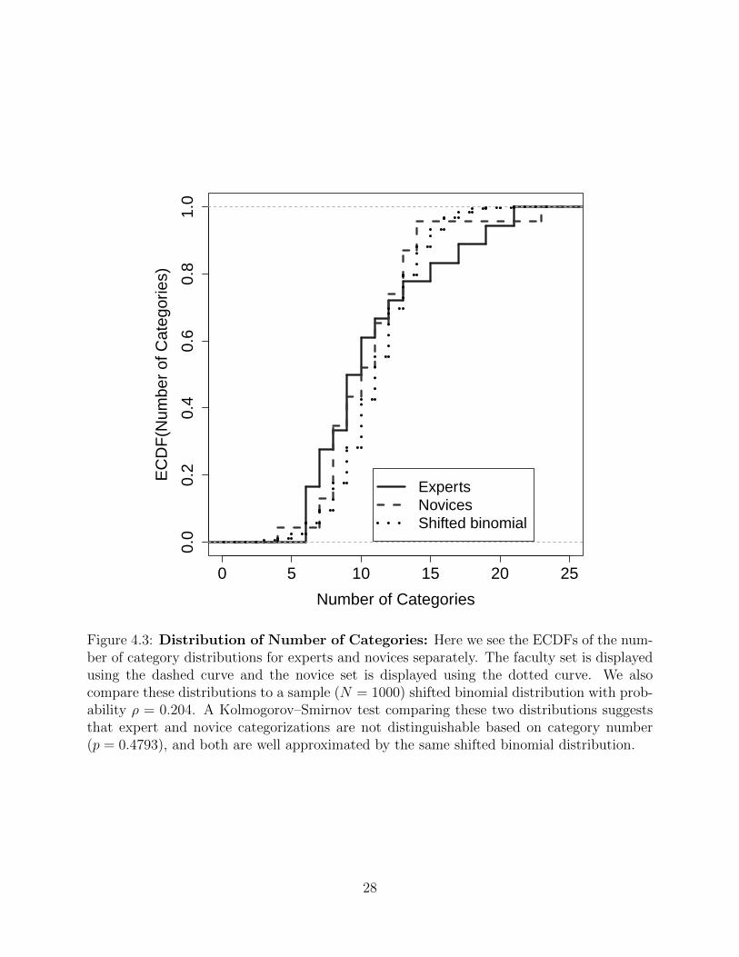
The “number of categories” is a frequently used macroscopic measure of card sorting distri-
butions and not yet particular to graph theory. Chi et al.’s experiment found that experts
and novices created, on average, the same number of categories, which is true also in our
study: experts created an average of 10.8±4.5 categories, while novices created 11.4±4.4 cat-
egories. The large standard deviations indicate a wide distribution of category counts, and
thus we decided to extend our comparison to the entire distributions, which includes differ-
ences in skewness or shape. For example, a Gaussian distribution and a bimodal distribution
with the same mean and standard deviation would be discriminated in our tests whereas
they would not be discriminated when only comparing averages. In order to compare two
distributions, we consider the Empirical Cumulative Distribution Function (ECDF), which
is calculated from each normalized distribution D(x) as follows:
ECDF (x) =
∫ x
−∞D(x′)dx′ (4.3)
For the category number distribution the ECDF (x) represents the fraction of sorters who
have x or less categories. We used the 2-sample Kolmogorov–Smirnov goodness-of-fit hypoth-
esis test (KS-test). The KS-test statistic is the maximum difference between two ECDFs.
Sample distributions from the same population have a known KS-test statistic distribution.
26

This allows for the calculation of a p-value much in the same way that a p-value is calculated
from a T-test. This p-value behaves in the usual way: If p > 0.05, then the distributions are
not statistically different at a 95% confidence interval. A KS-test comparing the ECDFs of
expert and novice number of categories (see Figure 4.3) demonstrated no statistically signif-
icant difference (p = 0.4793). This result confirms and expands Chi et al.’s result regarding
the average number of categories for experts and novices. Furthermore, we see that these
distributions are consistent with a binomial distribution.
The graph-theoretical equivalent of the number of categories is the number of maximal
cliques. A node is a member of a clique if it is connected to all of the other nodes in the
clique, and a clique is maximal if there is no other node which may be added to the clique.
To investigate the possible “collapse” of categories, we analyzed the ratio of categories to
maximal cliques for each sorter, and found that all but four sorters had exactly the same
number of maximal cliques as categories, which was not statistically significant (p-value=1.0).
4.3 Connectedness
The number of so-called 3-cycles macroscopically describes the connectedness of a graph,
and is the first graph theoretical measure we apply. A 3-cycle is a sub-graph of three vertices
where all vertices connect by edges. In our example, shown in Figure 4.1, one of the 24 3-
cycles is the sub-graph including vertices {1, 3, 5} because they are all connected by (at least)
one edge. However, the sub-graph including vertices {1, 2, 3} is not a 3-cycle because vertex 1
is not connected to vertex 2. This statistic is related to how often a sorter categorizes cards in
multiple piles. Contrary to the previous example where 7 of the 10 problems were categorized
twice, now consider the following example without any multiple categorization. Suppose the
27
0 5 10 15 20 25
0.0
0.2
0.4
0.6
0.8
1.0
Number of Categories
EC
DF
(Num
ber
of C
ateg
orie
s)
ExpertsNovicesShifted binomial
Figure 4.3: Distribution of Number of Categories: Here we see the ECDFs of the num-ber of category distributions for experts and novices separately. The faculty set is displayedusing the dashed curve and the novice set is displayed using the dotted curve. We alsocompare these distributions to a sample (N = 1000) shifted binomial distribution with prob-ability ρ = 0.204. A Kolmogorov–Smirnov test comparing these two distributions suggeststhat expert and novice categorizations are not distinguishable based on category number(p = 0.4793), and both are well approximated by the same shifted binomial distribution.
28
1 10 100 1000 10000
0.0
0.2
0.4
0.6
0.8
1.0
N3cycles
ecdf
(N3c
ycle
s)
ExpertsNovices
Figure 4.4: Number of 3-cycles: This is the distribution of the number of 3-cycles forexperts and novices. A Kolmogorov–Smirnov test suggests that experts and novices are notdistinguishable based on their 3-cycle distributions (p = 0.1584).
conservation of energy category has problems {1, 4, 7, 10}, the Newton’s Second Law category
has problems {2, 5, 8}, and the conservation of momentum category has problems {3, 6, 9}.
In this categorization, where there are no problems multiply categorized, there are only six
3-cycles. As such, the 3-cycle distribution is extremely useful for analyzing the connectedness
of graphs. A KS-test comparing the ECDFs of expert and novice 3-cycle distributions (see
Figure 4.4) demonstrated no statistically significant difference (p = 0.1584). This result was
expected because connectedness does not take problem identity into account.
29
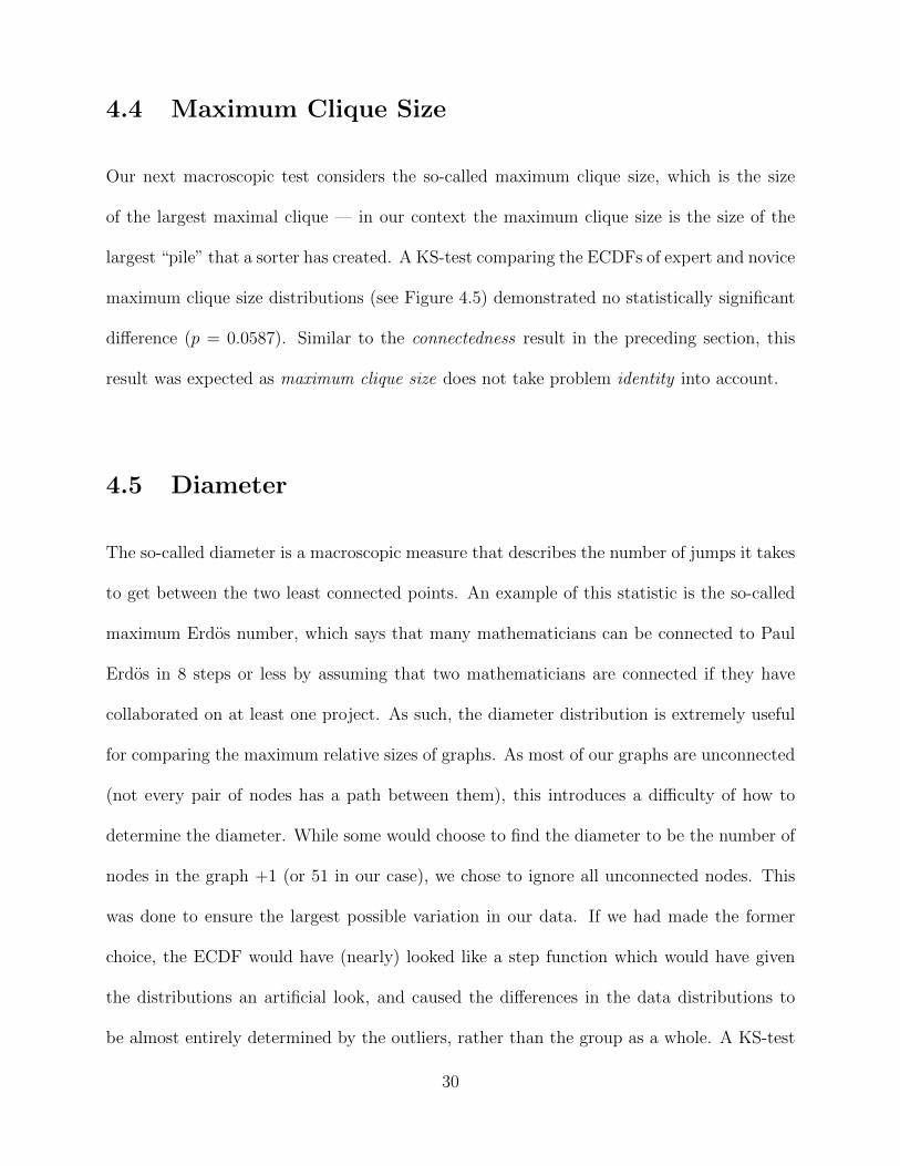
4.4 Maximum Clique Size
Our next macroscopic test considers the so-called maximum clique size, which is the size
of the largest maximal clique — in our context the maximum clique size is the size of the
largest “pile” that a sorter has created. A KS-test comparing the ECDFs of expert and novice
maximum clique size distributions (see Figure 4.5) demonstrated no statistically significant
difference (p = 0.0587). Similar to the connectedness result in the preceding section, this
result was expected as maximum clique size does not take problem identity into account.
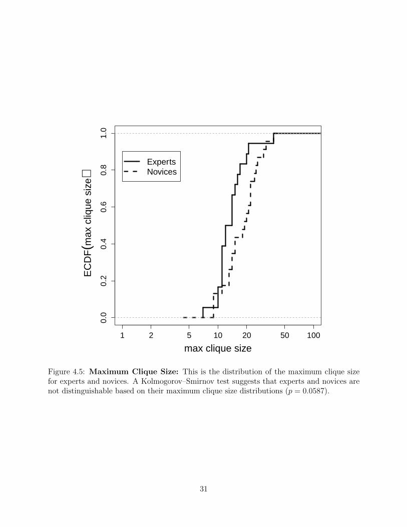
4.5 Diameter
The so-called diameter is a macroscopic measure that describes the number of jumps it takes
to get between the two least connected points. An example of this statistic is the so-called
maximum Erdos number, which says that many mathematicians can be connected to Paul
Erdos in 8 steps or less by assuming that two mathematicians are connected if they have
collaborated on at least one project. As such, the diameter distribution is extremely useful
for comparing the maximum relative sizes of graphs. As most of our graphs are unconnected
(not every pair of nodes has a path between them), this introduces a difficulty of how to
determine the diameter. While some would choose to find the diameter to be the number of
nodes in the graph +1 (or 51 in our case), we chose to ignore all unconnected nodes. This
was done to ensure the largest possible variation in our data. If we had made the former
choice, the ECDF would have (nearly) looked like a step function which would have given
the distributions an artificial look, and caused the differences in the data distributions to
be almost entirely determined by the outliers, rather than the group as a whole. A KS-test
30
1 2 5 10 20 50 100
0.0
0.2
0.4
0.6
0.8
1.0
max clique size
EC
DF(m
ax c
lique
siz
e)
ExpertsNovices
Figure 4.5: Maximum Clique Size: This is the distribution of the maximum clique sizefor experts and novices. A Kolmogorov–Smirnov test suggests that experts and novices arenot distinguishable based on their maximum clique size distributions (p = 0.0587).
31
0 1 2 3 4 5 6
0.0
0.2
0.4
0.6
0.8
1.0
diameter
EC
DF(d
iam
eter
)ExpertsNovices
Figure 4.6: Diameter: This is the distribution of the diameter of the experts and novices.A Kolmogorov–Smirnov test suggests that experts and novices are not distinguishable basedon their diameter distributions (p = 0.6432).
comparing the ECDFs of expert and novice diameter distributions (see Figure 4.6) demon-
strated no statistically significant difference (p = 0.6432). This result was also expected as
diameter does not take problem identity into account.
32

4.6 Average Path Length
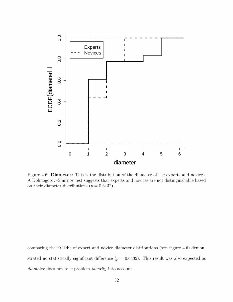
The average path length is a macroscopic measure that describes the average number of
jumps it takes to get between all unique pairs of points. As such, the distribution of average
path lengths may be used to compare the average relative sizes of the different graphs. The
calculation of the average path length is subject to the same difficulty due to unconnected
graphs as is the diameter. In this case, we chose to set the path length between unconnected
nodes to be 51, rather than ignoring them. In this setting, we feel that this measure includes
both the local structure of the graph and a measure of how unconnected the graph is as
well. As a result, we note that the range of average path length is much larger than the
diameter. However, a KS-test comparing the ECDFs of expert and novice average path
length distributions (see Figure 4.7) demonstrated no statistically significant difference (p =
0.3906). This result, combined with all of the previous results suggests that our hypothesis
that expert and novice categorizations can not be distinguished without taking problem
identity into account has merit.
33
0 20 40 60 80
0.0
0.2
0.4
0.6
0.8
1.0
average path length
EC
DF(a
vera
ge p
ath
leng
th) Experts
Novices
Figure 4.7: Average Path Length: This is the distribution of the average path length forexperts and novices. A Kolmogorov–Smirnov test suggests that experts and novices are notdistinguishable based on their average path length distributions (p = 0.3906).
34

Chapter 5
Categorization Models
This chapter develops a statistical model which seeks to find the common pattern behind
the common macroscopic sorting behavior of experts and novices. In creating this model we
choose only a three parameters to describe the group behavior: The number of questions
sorted (a parameter fixed by the experiment), the average number of categories, and the
multiple categorization parameter. As is customary in categorization experiments, a single
problem may be placed into more than one category, and the multiple categorization pa-
rameter describes the probability that multiple categorization occurs. Due to the fact that
the individual multiple categorization probability decreases with the individual number of
categories created, this reinforces the “stacker” vs. “spreader” interpretation.
All of the macroscopic statistical measures, that is, measures which dealt with just the
groups of cards and not the individual cards and their identities, yielded no significant
distinction between expert and novice sorters. For now, visualizing the data was successful
in quickly recognizing outliers (subjects who sort differently), but those outliers were not
necessarily more prevalent among experts or novices. We now aim to construct a model
35
of the categorization process that has the same macroscopic and visual properties as our
sample experimental data. Along the way, we learn more about human behavior during
categorization tasks.
We started out by using two standard models frequently used in graph theory literature.
Unfortunately, neither of these two standard models reproduces the data, in spite of the fact
that they are generally considered complementary. We thus created our own model, which
generated more realistic model data.
5.1 Standard Erdos-Renyi and Barabasi Models
An Erdos-Renyi model generates a “uniform” graph, that is a graph where any two vertices
have a certain fixed probability of being connected [28]. Uniform graphs may be generated
as random realizations of a model having two parameters: the number of nodes and the
probability that nodes will connect. Barabasi graphs, a kind of a “small-world” graph often
used to model social networking connections[29], is created by adding one node at a time, and
connecting this new node with the existing nodes on the graph with a probability related to
the number of edges already connected to each node P ∝ Na+ b. The model for a Barabasi
graph has three parameters, the number of nodes in the graph, the probability to connect
to a node with no other connections (b), and the power (a) by which the number of edges
already connected to a node (N) is raised. We describe next the statistical comparison and
analysis of graphs generated by these models to the graphs generated by our human sorters.
First, we considered the Erdos-Renyi model. See Figure 5.1 for examples of Erdos-Renyi
graphs. In order to determine the best input parameters for our model we optimized these
parameters using the standard algorithm “optim” found in R[24]. This was done by calculat-
36
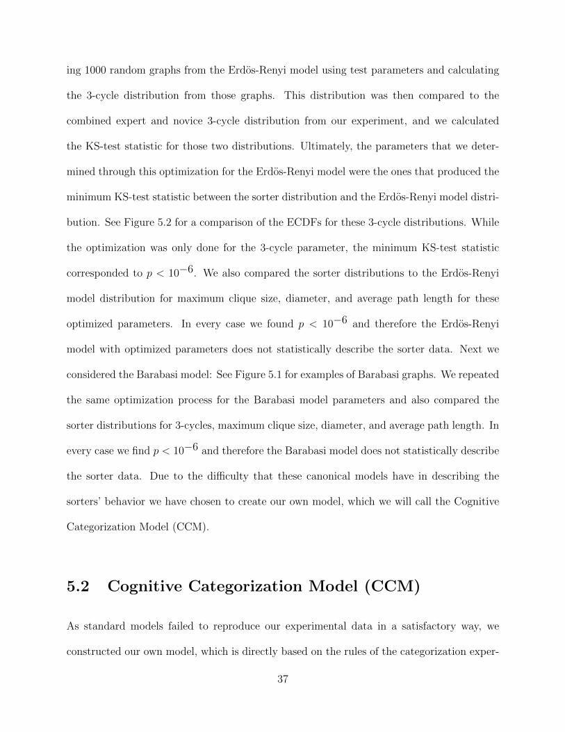
ing 1000 random graphs from the Erdos-Renyi model using test parameters and calculating
the 3-cycle distribution from those graphs. This distribution was then compared to the
combined expert and novice 3-cycle distribution from our experiment, and we calculated
the KS-test statistic for those two distributions. Ultimately, the parameters that we deter-
mined through this optimization for the Erdos-Renyi model were the ones that produced the
minimum KS-test statistic between the sorter distribution and the Erdos-Renyi model distri-
bution. See Figure 5.2 for a comparison of the ECDFs for these 3-cycle distributions. While
the optimization was only done for the 3-cycle parameter, the minimum KS-test statistic
corresponded to p < 10−6. We also compared the sorter distributions to the Erdos-Renyi
model distribution for maximum clique size, diameter, and average path length for these
optimized parameters. In every case we found p < 10−6 and therefore the Erdos-Renyi
model with optimized parameters does not statistically describe the sorter data. Next we
considered the Barabasi model: See Figure 5.1 for examples of Barabasi graphs. We repeated
the same optimization process for the Barabasi model parameters and also compared the
sorter distributions for 3-cycles, maximum clique size, diameter, and average path length. In
every case we find p < 10−6 and therefore the Barabasi model does not statistically describe
the sorter data. Due to the difficulty that these canonical models have in describing the
sorters’ behavior we have chosen to create our own model, which we will call the Cognitive
Categorization Model (CCM).
5.2 Cognitive Categorization Model (CCM)
As standard models failed to reproduce our experimental data in a satisfactory way, we
constructed our own model, which is directly based on the rules of the categorization exper-
37
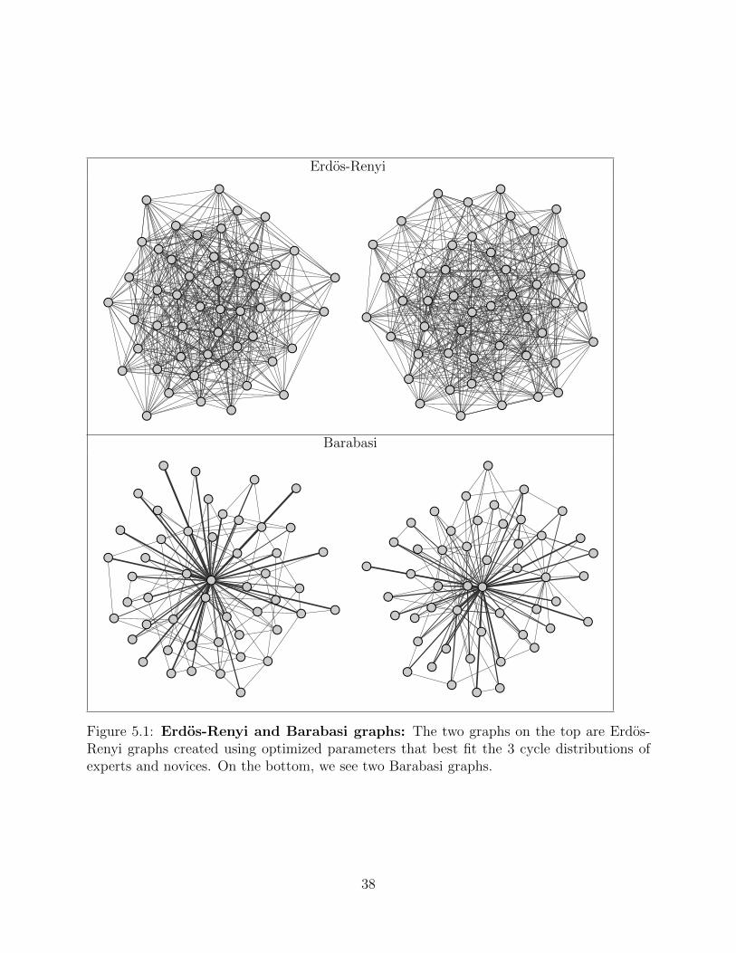
Erdos-Renyi
●
●
●
●
●
●
●
●●
●
●
●
●
●
●
●
●
●
●
●
●
●
●
●
●
●
●
●
●
●●
●
●
●
●
●
●
●
●
●●
●
●
●
●●
●
●
●
●
●
●
●
●●
●
●
●
●
●
●
●
●
●
●
●
●
●
●●
●
●
●
●
●
●
●
●
●
●
●
●
●
●
●
●
●
●
●
●
●
●
●
●
●
●
●
●
●
●
Barabasi
●●
●
●
●
●
●
●
●
●
●
●
●
●
●
●
●
●
●
●
●
●
●
●
●
●●
●
●●
●
●
●
●
●
●
●
●
●
●
●
●
●
●
●
●
●
●
●
●
●●●
●
●
●
●
●
●
●
●
●
●●
●●
●
●
●
●●
●
●●
●
●
●
●
●
●
●
●
●●
●
● ●
●
●
●
●
●●
●
●
●
●
●
●
●
Figure 5.1: Erdos-Renyi and Barabasi graphs: The two graphs on the top are Erdos-Renyi graphs created using optimized parameters that best fit the 3 cycle distributions ofexperts and novices. On the bottom, we see two Barabasi graphs.
38
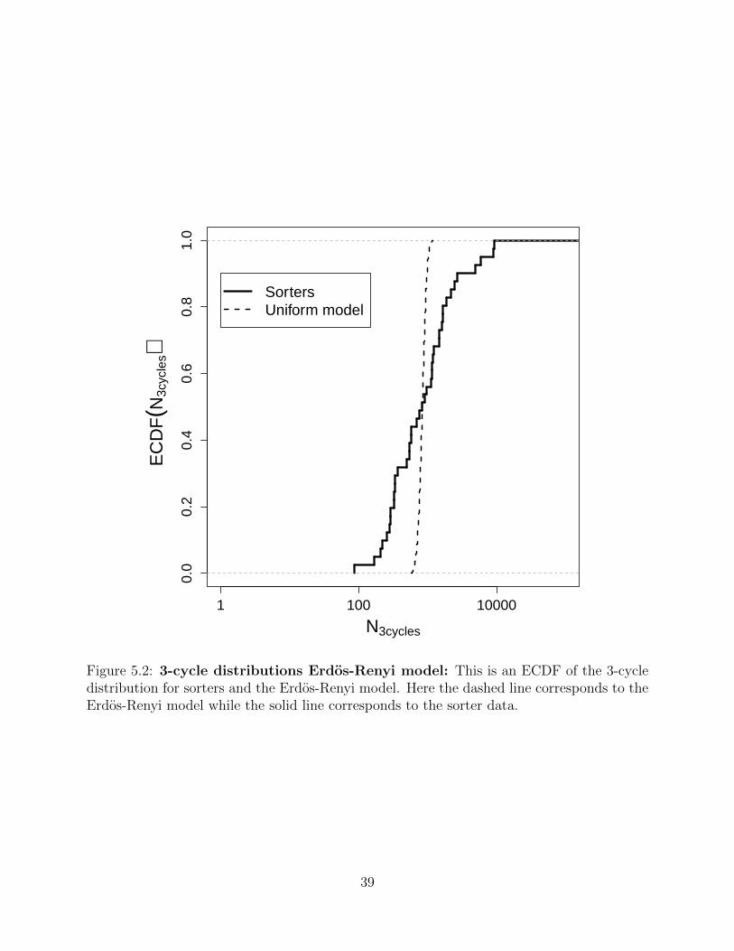
1 100 10000
0.0
0.2
0.4
0.6
0.8
1.0
N3cycles
EC
DF(N
3cyc
les)
SortersUniform model
Figure 5.2: 3-cycle distributions Erdos-Renyi model: This is an ECDF of the 3-cycledistribution for sorters and the Erdos-Renyi model. Here the dashed line corresponds to theErdos-Renyi model while the solid line corresponds to the sorter data.
39
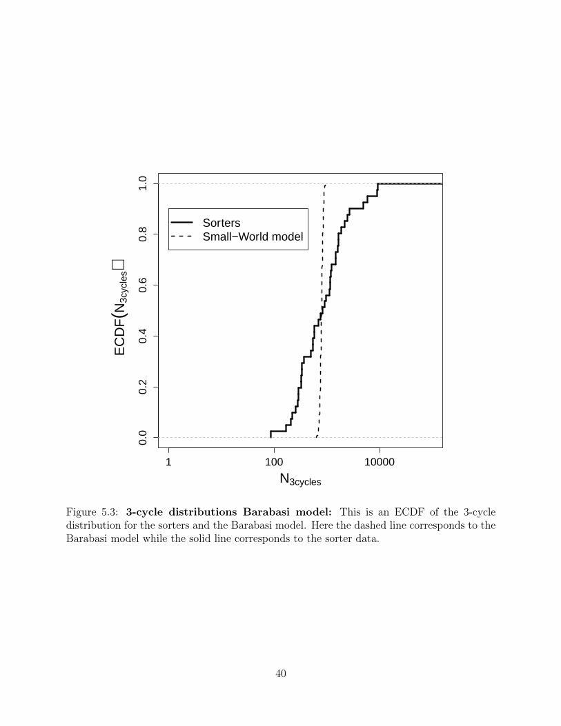
1 100 10000
0.0
0.2
0.4
0.6
0.8
1.0
N3cycles
EC
DF(N
3cyc
les)
SortersSmall−World model
Figure 5.3: 3-cycle distributions Barabasi model: This is an ECDF of the 3-cycledistribution for the sorters and the Barabasi model. Here the dashed line corresponds to theBarabasi model while the solid line corresponds to the sorter data.
40

iment:
1. All questions must be put into a category.
2. All categories must have at least one question in them.
3. A question may fall into more than one category.
The latter rule is mathematically cumbersome, but had to be included since it is standard
procedure in most experiments, including the one that was the base of our sample data in
the previous section.
Our new model, which we call the Cognitive Categorization Model (CCM), has three
parameters: The first parameter of the CCM model (Q) represents the number of questions
that are being categorized in the experiment. The second parameter is the average number of
categories determined by a sorter. As we described in Subsection 4.2, a shifted binomial dis-
tribution fits the category number data rather well. A binomial distribution is the “weighted
coin” distribution — if you flip a weighted coin N times, what is the probability that you
will get “heads” k times? In principle, one can flip a coin N times and get tails every time.
By Rule #1, we do not want to allow zero categories, therefore we must introduce a shift.
It would also be senseless to create more categories than questions, so we wish to choose
a number of categories from between 1 and Q. The simplest way to do this is to generate
a number from the binomial distribution between 0 and Q − 1 and then add 1 to each of
these randomly generated values. The probability of success is chosen to correspond to the
final average number of categories. The final parameter is the probability to categorize a
card into more than one pile. After each problem has been sorted into a single pile, the
algorithm tests whether that problem should be sorted into other categories as well. Our
41
model, with 2 free parameters is on par with the Erdos-Renyi model (1 free parameter) and
the Barabasi model (2 free parameters). In addition to the fact that the CCM parameters
are interpretable, the small number of CCM parameters makes this model parsimonious.
Appendix shows the pseudocode for this model. In our code, we implement multiple
categorization by generating a random number between zero and one and comparing that
number to our multiple categorization probability. However, there are a number of ways that
we can model the multiple categorization probability. The simplest way is to allow every
sorter to have a uniform probability and say that some percentage of the time a card will be
split again. So for this model the multiple categorization probability is constant (CCMv1):
Pmultiple = β1 (5.1)
where β1 is a constant between zero and one which applies to the entire population. Another
way that we consider assumes that a penalty is incurred whenever a card is split (CCMv2):
Pmultiple = βN2 (5.2)
where β2 is a constant between zero and one which applies to the entire population and N
is the number of times that a problem has already been categorized by a random sorter.
Finally, we consider a model where the multiple categorization probability depends on the
number of categories (C) that a sorter has selected which was determined by the binomial
distribution (CCMv3):
Pmultiple = βC3 (5.3)
42
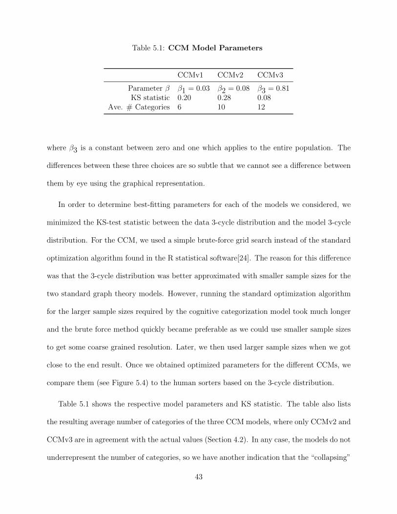
Table 5.1: CCM Model Parameters
CCMv1 CCMv2 CCMv3
Parameter β β1 = 0.03 β2 = 0.08 β3 = 0.81KS statistic 0.20 0.28 0.08
Ave. # Categories 6 10 12
where β3 is a constant between zero and one which applies to the entire population. The
differences between these three choices are so subtle that we cannot see a difference between
them by eye using the graphical representation.
In order to determine best-fitting parameters for each of the models we considered, we
minimized the KS-test statistic between the data 3-cycle distribution and the model 3-cycle
distribution. For the CCM, we used a simple brute-force grid search instead of the standard
optimization algorithm found in the R statistical software[24]. The reason for this difference
was that the 3-cycle distribution was better approximated with smaller sample sizes for the
two standard graph theory models. However, running the standard optimization algorithm
for the larger sample sizes required by the cognitive categorization model took much longer
and the brute force method quickly became preferable as we could use smaller sample sizes
to get some coarse grained resolution. Later, we then used larger sample sizes when we got
close to the end result. Once we obtained optimized parameters for the different CCMs, we
compare them (see Figure 5.4) to the human sorters based on the 3-cycle distribution.
Table 5.1 shows the respective model parameters and KS statistic. The table also lists
the resulting average number of categories of the three CCM models, where only CCMv2 and
CCMv3 are in agreement with the actual values (Section 4.2). In any case, the models do not
underrepresent the number of categories, so we have another indication that the “collapsing”
43

1 100 10000
0.0
0.2
0.4
0.6
0.8
1.0
N3cycles
EC
DF(N
3cyc
les)
SortersCCM v1CCM v2CCM v3
Figure 5.4: 3-cycle distributions Here we see the 3-cycle distributions for the differentCCMs. The model that fits the best is v3 (Equation 5.3), where the multiple categorization
probability is βC .
44
of categories (end of Section 4.1) does not appear to be an issue with the actual data.
Overall, we found that the best fitting CCM is CCMv3, which has a multiple categorization
probability that depends on the number of categories (Equation 5.3). Figure 5.5 shows some
example CCMv3 graphs; these CCM graphs look much more like the graphs of the human
sorters seen in Fig. 4.2 than the Erdos-Renyi and Barabasi graphs in Fig. 5.1.
The success of this model gives us insight into the behavior of our sorters: the probability
to categorize a single problem in multiple categories is different for each person, and that
probability actually decreases with the number of categories that are created. This model
prediction is supported by an observation we made of our sorters. We observed two different
sorter behaviors while they worked on the categorization task. It seemed like some people
were resolved to make as few piles as possible, we will call these people “stackers.” Stackers
were more likely to put a problem in multiple categories, deciding that putting a problem
into two piles was a better decision than making a new category. As a result a stacker’s
groups tend to be large and inclusive. The other group of people would spread the problems
out on the table that they were working on, we will call these people “spreaders.” Spreaders
were less likely to put a problem in multiple categories, deciding that making a new category
was a better decision than putting a problem into two piles. As a result a spreader’s groups
tend to be small and exclusive.
45
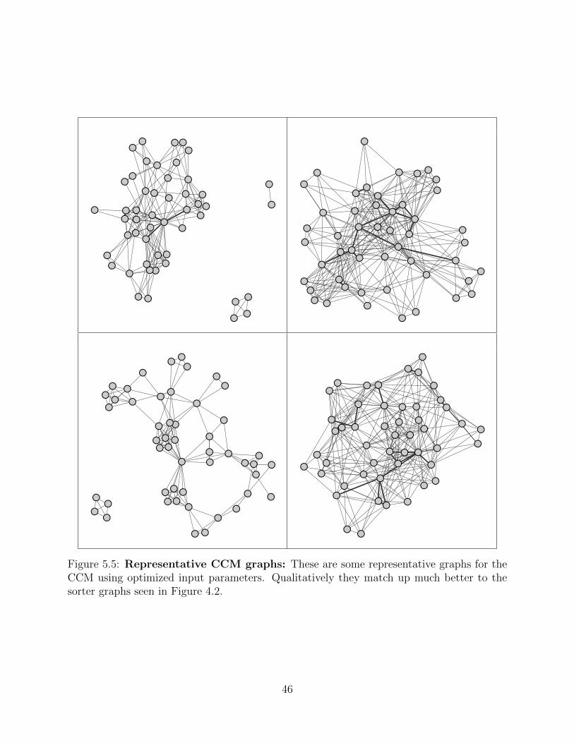
●●●
●
●●
●
●●
●
●
●
●
●
●
●
●
●
●
●●
●
●
●
●
●
●●
●
●
●
● ●
●
●
●
●
●
●
●
●●
●
●
●
●●
●
●
●
●
●●
●
●
●
●●
●
●
●
●
●
●
●
●
● ●
●
●
●
●
●
●
●
●
●
●
●
●
●
●●
●
●
●
●
●
●
●●
●
●
●
●
●
●
●
●
●
●
●
●
●
●
●
●
●
●
●
● ●
●
●
●
●
●
●
●
●
●
●
●
●
●●
●
●
●
●●
● ●
●
●
●
●
●
●
●
●
●
●
●
●
●●
●●
●
●
●
●●
●
●
● ●
●
●
●
●●
●
●
●
●
●
●
●
●
●
●
●
●
●
●
● ●
●
●
●
●
●
●
●
●
●●
●
●
●
●
●
●
●
●
●
●
●
Figure 5.5: Representative CCM graphs: These are some representative graphs for theCCM using optimized input parameters. Qualitatively they match up much better to thesorter graphs seen in Figure 4.2.
46

Chapter 6
Microscopic Properties of Sample
Experimental Data
This chapter details how to compare any two categorization graphs to each other using a
distance metric we developed and will visualize the relative position of sorters using Principal
Components Analysis (PCA) [6]. This visualization technique also confirms the “stacking”
and “spreading” behavior observed as the largest source of variation in our categorization
experiment. However, the second largest source of variation found by the PCA is due to
expertise. This finding suggests that the experiment of Chi et al. has been difficult to
replicate because the largest source of variation was not due to expertise. We explore next
why a particular set of problems would discriminate experts from novices, while others do
not, by considering many subsets of the large problem set categorized by the sorters.
47

6.1 Distance Metric
We now create a distance metric as a microscopic measure to compare two sorters to each
other. There are several existing distance metrics that will compare two different sortings,
including statistical indices such as the Rand Index [30] which can be converted into a
distance metric. However, in searching for existing statistical methods that will work for our
categorization exercise, we found none that obeyed the rules of our “categorization game,”
especially the third rule. The Rand index merely counts the number of “agreements.” This
may be calculated for any two categorizations. However similarity indicies that are not
corrected for chance agreements are not as reliable for creating a sort of measuring stick for
measuring a “distance” between two categorizations [31, 32]. For this reason Hubert and
Arabie created an adjustment to the Rand index. However this adjustment requires that
the sub-groups are disjoint, eliminating any utility that the adjusted Rand index has for
our study and other similar studies which allow multiple categorization. This story may
be repeated for any one of the other statistical indicies that we could find in the statistics
literature, and after some consideration, we decided that we needed to invent a new method
for analyzing this type of data.
Our distance metric will bypass this difficulty as it is a direct distance metric and not a
similarity index. The distance metric is determined by considering the weighted adjacency
matrix for each reviewer, and it compares any two graphs generated by two reviewers as long
as they have the same number of nodes (which they would for identical card sets). Each
element of the weighted adjacency matrix Xr for each reviewer r is:
Xrij = number of edges between problems i and j (6.1)
48
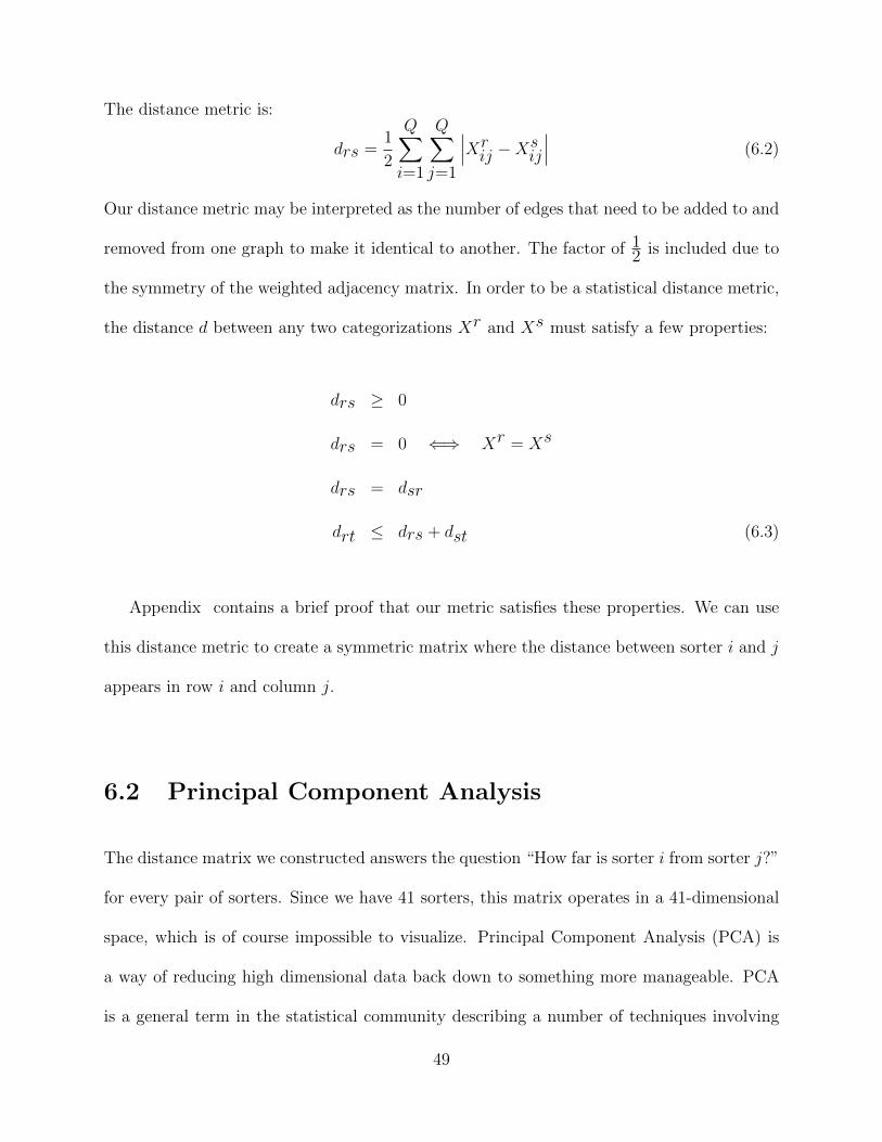
The distance metric is:
drs =1
2
Q∑i=1
Q∑j=1
∣∣∣Xrij −Xsij∣∣∣ (6.2)
Our distance metric may be interpreted as the number of edges that need to be added to and
removed from one graph to make it identical to another. The factor of 12 is included due to
the symmetry of the weighted adjacency matrix. In order to be a statistical distance metric,
the distance d between any two categorizations Xr and Xs must satisfy a few properties:
drs ≥ 0
drs = 0 ⇐⇒ Xr = Xs
drs = dsr
drt ≤ drs + dst (6.3)
Appendix contains a brief proof that our metric satisfies these properties. We can use
this distance metric to create a symmetric matrix where the distance between sorter i and j
appears in row i and column j.
6.2 Principal Component Analysis
The distance matrix we constructed answers the question “How far is sorter i from sorter j?”
for every pair of sorters. Since we have 41 sorters, this matrix operates in a 41-dimensional
space, which is of course impossible to visualize. Principal Component Analysis (PCA) is
a way of reducing high dimensional data back down to something more manageable. PCA
is a general term in the statistical community describing a number of techniques involving
49

the singular value decomposition. To visualize our data, we did a singular value decomposi-
tion on the distance matrix. By applying the singular value decomposition to the distance
matrix we perform a change of base so that the largest amount of variation is in the first
principal component (PC1), the second largest amount of variation is in the second principal
component (PC2), and each subsequent component explains less variation than the previous
component. This analysis is then projected out onto fewer spatial dimensions, using only
the most influential base vectors as a new reduced base.
Contrary to many applications of PCA, ours will not independently allow for interpreta-
tion of the groups of sorters that are separated by the analysis. This is due to the nature of
the matrix being analyzed by the PCA. In general, PCA assumes that each row is an obser-
vation and each column is a property. For example, in astronomy one could look at several
properties of stars (e.g. the temperature, the metallicity, the absolute brightness, etc.) for
many different stars. The principal components themselves (PC1, PC2, etc.) are linear com-
binations of these properties. Because of the interpretability of the principal components,
PCA is often able to explain the source of variation between groups of data. However in
our application, that is not true. This is because the properties are the distances from each
sorter and not some fundamental property of each sorter. Therefore, the principal compo-
nents are linear combinations of sorters, and are not able to aid in interpreting the source
of the variation between these sorters. Any interpretation of the principal components that
we will be able to do is therefore a function of our ability to explain that variability using
other complimentary analysis methods.
For a PCA to be considered successful, the majority of variation must be explained
with just a few components. In our case, taking just the first two components explains
50

approximately 87% of the variability in our dataset. We thus focus on this reduced-dimension
PCA, which can easily be visualized in Figure 6.1. We can now visualize our sorters and easily
interpret what we see. The question of what sorter characteristic results in what behavior of
PC1 and PC2 is lost in a 41-dimensional rotation and subsequent projection. In other words,
this abstract representation of microscopic data (the distance matrix strongly depends on
problem identities) does not boil down to a simple linear combination of macroscopic features.
An early concern was that the outliers (subjects who sort very differently than the ma-
jority, e.g., sorter 16 in Fig. 4.2, who is also clearly distinguishable in Fig. 6.1) might strongly
influence the PCA, and so the complete analysis was run with and without these particular
sorters. We found that the difference that these outliers made in the outcome of the PCA
was not significant; in other words, the method we are employing is robust against “noise”
in the data introduced by occasional outliers. We thus decided to keep the outliers within
the data set.
Making sense of PC1 and PC2 is where the previous work on graph visualization (Sec-
tion 4.1) and analysis (Sections 4.2 through 4.6), combined with the interpretation of the
CCM (Section 5.2) comes together. We can look at the relative placement of our sorters
by the PCA, visually analyze their graphs, and attempt an interpretation of the abstract
sources of variation found by the PCA. The expert and novice identity of each sorter is a
variable known only to us and not a factor in determining the placement of the sorters by
the PCA
Analyzing the sorters in order of increasing PC1-coordinate (Fig. 6.1, left panel) shows
that this coordinate does not distinguish experts from novices. In other words, most variance
in the data is not related to the expert or novice identity of the sorters. Instead, when
51
analyzing the graphs associated with the subjects, it turns out that PC1 mostly reflects the
“stacker” versus “spreader” behavior identified through our CCM (Section 5.2), which is
quite independent of being an expert or a novice. Based on this result, one could argue that
card-sorting experiments most strongly measure how individuals sort, and may thus be more
reflecting of what that individual’s office or the file system of his or her personal computer
looks like than whether or not he or she is a physics expert.
The expert/novice distinction only shows up in PC2. Going along the PC2-axis in the
left panel of Figure 6.1, one finds more experts with a high PC2 and more novices with a
low PC2. At this point we are both paradoxically hopeful—because expert-novice variation
shows up in this PC2—and deeply unsatisfied—because we have no indication about the
source of this variation. So far, we have a set that can discriminate experts from novices. Up
until this point we have ignored the single experimental “knob” that we can use to control
this experiment: The problems themselves. In the next two chapters we will attempt to
explain the source of this discrimination between experts and novices by quantifying that
discrimination and studying the properties of the problems themselves.
52
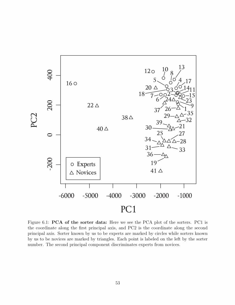
400
-200
020
0
PC2
-6000 -1000-2000-3000-4000-5000
PC1
NovicesExperts
36
2016
12
38
40
22
1310
1941
2725283331
34
29
85
37
39
7
3532
69
24
26
4 17
2130
111432 15
231
18
Figure 6.1: PCA of the sorter data: Here we see the PCA plot of the sorters. PC1 isthe coordinate along the first principal axis, and PC2 is the coordinate along the secondprincipal axis. Sorter known by us to be experts are marked by circles while sorters knownby us to be novices are marked by triangles. Each point is labeled on the left by the sorternumber. The second principal component discriminates experts from novices.
53

●
●
●
●●
●●
●●
● ● ● ● ● ● ● ● ● ● ● ● ● ● ● ● ● ● ● ● ● ● ● ● ● ● ● ● ● ● ● ●
0 10 20 30 40
5060
7080
9010
0
Eigenvalue rank
Cum
ulat
ive
rela
tive
impo
rant
ce o
f eac
h ei
genv
alue
Figure 6.2: Validating the use of PCA on the sorter data: This is a plot of thecumulative relative importance of each subsequent principal component. This shows thatmost of the variation is well-described by the first two principal components. Therefore usingPCA for dimension reduction is an appropriate choice for this data.
54

Chapter 7
Parameterizing Subsets
In this chapter we discuss the different statistics used to describe the problem sets. These
include the cognitive and contextual features of the problems as well as the ability that a
subset has to discriminate expert and novice sorters. The contextual features of the problems
include a problem’s chapter and difficulty. The discriminatory properties of subsets are found
by using both parametric and non-parametric tests which compare the PCA coordinates of
the expert and novice groups.
We found that the most salient feature of problem categorizations, that is, the first
principal component of the PCA, is related to the sorting behavior of the individuals, a
personality trait we termed “stacker” versus “spreader” [6]. The meaning of this component
was easy to recognize, as it exhibited itself in the stark visual differences between the the
sorters’ categorization graphs. A stacker tended to generate a few large piles of cards with
the same problem being a member of several piles. In contrast, a spreader tended to generate
many fine-grained small piles and would rarely allow a single problem to be a member of
several piles. Expertise only came in second, as the distinction between experts and novices is
55

exhibited by the second principal component. Unfortunately, due to the multi-dimensional
nature of the Principal Component Analysis and missing visual clues in the graphs, we
were unable to infer the source of this variability. However, all indications are that this
behavior is problem-specific. After all, variability in student performance while working on
problems in relativity [16] and motion [17] is well-documented. It is reasonable to believe
that this problem-dependent nature of student reasoning extends from solving problems to
the categorization behavior of sorters, as it depends on the particular problems being used.
What is the composition of a minimal ideal subset? What problem features need to be
present? In other words, instead of picking random problems from the back of chapters
in textbooks, how much does a problem set need to be “rigged” in order to be effective in
discriminating experts and novices?
Additional evidence for the importance of careful question selection—or “rigging”—was
given by Veldhuis [2], who also attempted to verify the result of Chi et al.. Veldhuis created
four different categorization sets. The first set was created in an attempt to mimic the Chi
et al. problem set [3], and the second was a control set with a similar collection of end-of-
chapter problems. In contrast, the third and fourth sets were carefully constructed so that
each problem had only a single physics principle and a single surface feature from a set of four
principles and four surface features [2]. The fourth set was also “rigged.” It had the same
number and type of cards, but only two surface and two conceptual features. Veldhuis could
not draw a conclusion from the categorizations from his first two problem sets. However,
sets 3 and 4 agreed with Chi et al. in that experts categorize problems based on physics
principles while novices show a “more complex behavior.” [2, 3]. Where on the “rigging
continuum” do problem sets need to be constructed in order to achieve measurable results?
56
Also, can Veldhuis’ result be generalized to more complex problems—that is, problems with
more than one physics principle and more than one surface feature?
We explore on a microscopic level why particular sets of problems would discriminate
experts from novices while others do not, looking at the individual properties of the included
problems. The main strategy of our approach is to pick subsets out of our large set of
problems, determine how well they distinguish experts from novices, and then examine their
composition based on a number of pedagogical and contextual features. Combinatorics
dictate that we can effectively sample the entire population for small subsets only, while
for larger subsets, we use simulated annealing to optimize selected “starter sets.” We do
not propose that subset analysis is equivalent to actually giving our sorters many subsets to
categorize. Yet, we believe that subset analysis is still able to find the features that should
be present in an ideally “rigged” problem set.
7.1 Experimental Parameters
Previously, we designed and carried out a card-sorting experiment on physics experts and
novices at Michigan State University, adhering to the experimental method of Chi et al.
as closely as possible [6]. A total of 18 physics professors and 23 novices participated in
our study. All of the novices had completed at least the first semester of an introductory
physics course at MSU. We gave each sorter a set of 50 problems to sort based on “similarity
of solution,” explicitly following the prompt of Singh [7]. Each sorter categorized his or
her problems and recorded the groups and group names in a separate packet. Multiple
categorization, i.e., putting a single card into more than one category, was allowed, but not
expected.
57

●
●●
●●
●●
●
●
●
●
●
●
●
●
●
●●
−6000 −5000 −4000 −3000 −2000 −1000
−20
00
200
400
PC1
PC
2
● ExpertsNovices
Figure 7.1: Problem Dependence of PCA (Top) This is the PCA plot of the sorters forthe entire set of problems from our previous study [6]. Both a Cramer’s test (p = 0.048)
and a Hotelling’s test (p < 10−5) find the expert and novice groups to be distinct at a95% confidence level. PC1 is the coordinate along the first principal axis, and PC2 is thecoordinate along the second principal axis. Sorters known by us to be experts are markedby circles while sorters known by us to be novices are marked by filled triangles. The secondprincipal component discriminates experts from novices.
58
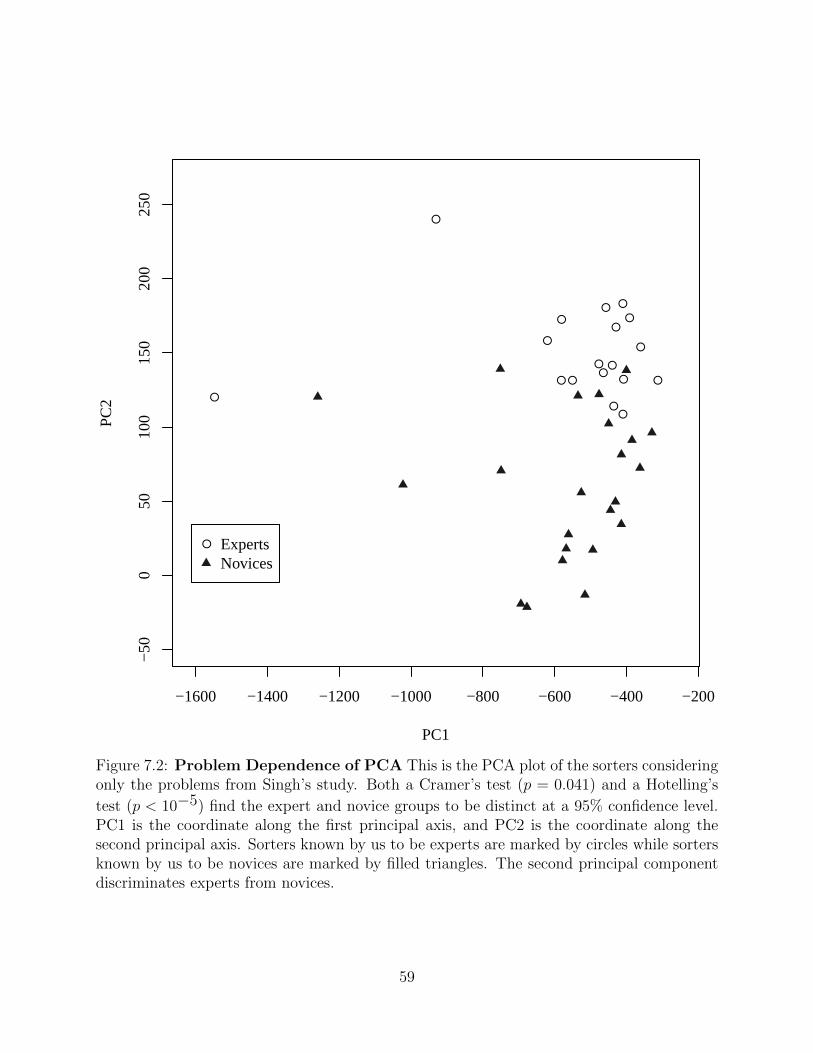
●
●
●
●
●
●
● ●
●
●
●
●
●●
●
●
●
●
−1600 −1400 −1200 −1000 −800 −600 −400 −200
−50
050
100
150
200
250
PC1
PC
2
● ExpertsNovices
Figure 7.2: Problem Dependence of PCA This is the PCA plot of the sorters consideringonly the problems from Singh’s study. Both a Cramer’s test (p = 0.041) and a Hotelling’s
test (p < 10−5) find the expert and novice groups to be distinct at a 95% confidence level.PC1 is the coordinate along the first principal axis, and PC2 is the coordinate along thesecond principal axis. Sorters known by us to be experts are marked by circles while sortersknown by us to be novices are marked by filled triangles. The second principal componentdiscriminates experts from novices.
59
7.1.1 Problem Set Creation
We constructed our initial large set of problems such that was diverse in terms of both
content and cognitive demands. We considered two traditional measures, the chapter which a
problem is in (using Walker’s textbook[4] as a guide) and the problem difficulty as measured
by the number of “dots” a problem has. We also included the taxonomic classification
according to the Taxonomy of Introductory Physics Problems (TIPP) [5]. The TIPP is useful
because it considers two dimensions or knowledge domains, one for declarative knowledge
(information) and the other for procedural knowledge (mental procedures) [5]. See Table
7.2 for a list of the TIPP levels included in our study. Higher levels were not included
because they are more suited to research projects rather than homework problems [5]. Each
problem was therefore classified along four feature dimensions: the chapter in which the
problem could be found (CHAP), the problem difficulty (DIFF), as well as the highest
complex cognitive process necessary to solve it for both declarative knowledge (TIPP-D)
and procedural knowledge (TIPP-P). We did not consider the surface features (as used by
Veldhuis [2]) of the problems, since those are not quantifiable.
7.1.2 Expert-Novice Differentiation
Our initial experiment found that experts and novices were separated by the second principal
component. While this is visually possible based on figures like Fig. 7.1 and Fig. 7.2, where
the experts congregate higher on the PC2 axis than the novices, we needed a way to quantify
this differentiation. We considered three statistical tests: the Hotelling’s test [33], the Cramer
test [34], and the Average Rate of Correct Classification (ARCC) [35]. The Hotelling’s test
is a standard test used to compare two groups of multivariable data, which assumes that
60
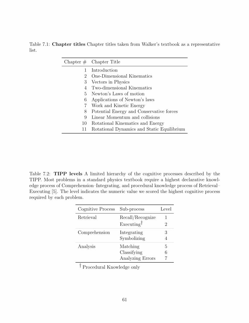
Table 7.1: Chapter titles Chapter titles taken from Walker’s textbook as a representativelist.
Chapter # Chapter Title
1 Introduction2 One-Dimensional Kinematics3 Vectors in Physics4 Two-dimensional Kinematics5 Newton’s Laws of motion6 Applications of Newton’s laws7 Work and Kinetic Energy8 Potential Energy and Conservative forces9 Linear Momentum and collisions
10 Rotational Kinematics and Energy11 Rotational Dynamics and Static Equilibrium
Table 7.2: TIPP levels A limited hierarchy of the cognitive processes described by theTIPP. Most problems in a standard physics textbook require a highest declarative knowl-edge process of Comprehension–Integrating, and procedural knowledge process of Retrieval–Executing [5]. The level indicates the numeric value we scored the highest cognitive processrequired by each problem.
Cognitive Process Sub-process Level
Retrieval Recall/Recognize 1
Executing† 2
Comprehension Integrating 3Symbolizing 4
Analysis Matching 5Classifying 6Analyzing Errors 7
† Procedural Knowledge only
61

each group’s distribution of these data is elliptical [33]. The Cramer test is a non-parametric
analog of the Hotelling’s test, that is, it does not assume a distribution shape [34]. The
ARCC is a statistical test which relies on Linear Discriminant Analysis to determine how
well experts and novices are separated by the PCA. We combined all of these measures into
a Canonical Correlation Analysis (CCA) [36]. A CCA quantifies the relationship between
the predictor variables (in our case the problem statistics) to the explanatory variables (the
sorter discrimination statistics). Because CCA assumes linear relationships between the
predictor variables and the response variables, we did a log transformation on all of our
variables in order to linearize power-law relationships and symmetrize skewed distributions.
When analyzing the results of the CCA, we found that the Cramer statistic was an order of
magnitude more important than the Hotellings and ARCC statistics. Thus, we ended up just
using the Cramer statistics as the CCA for this study. In order to determine which problem
properties are most important for predicting sorter discrimination, we found the variability
explained by each problem feature dimension (CHAP, DIFF, TIPP-D, and TIPP-P) in this
manner:
varstat =corstat∑
stats corstat(7.1)
where corstat is the correlation coefficient found by calculating a CCA for each group of prob-
lem statistics with the sorter discrimination statistics and the summation in the denominator
is done over the groups of statistics.
62
Chapter 8
Subset Analysis: Data Mining the
Categorization Graphs
In this chapter, we discuss the results of this subset analysis and determine which properties
are important in discriminating experts from novices in a categorization experiment. We
discuss the importance, not only of problem content, but requiring sorters to categorize
problems which require diverse solution types and including simpler problems, rather than
the most difficult problems.
Can subsets be as effective as the complete set of 50 cards? As a proof of concept, we
have compared the sorter visualizations from the entire dataset from our previous study [6]
to the subset of problems within that set which we obtained from Singh’s study [7]. As you
can see in Figure 7.1 and Figure 7.2, the two visualizations have similar properties. Natu-
rally, the sorters have different relative positions, as our distance metric, and consequently
our visualization method, was designed to compare categorizations on a microscopic—or
problem-specific—level. However, the overall level of expert-novice discrimination is similar,
63
so the smaller carefully chosen subset would have been sufficient to discriminate experts from
novices.
8.1 Monte Carlo analysis
When forming subsets of our 50-problem set, combinatorics limit the sizes of subsets for
which we can explore possible combinations. We analyzed 40000 5-problem subsets and
275000 10-problem subsets of our original 50-problem set. Due to the highly parallelizable
nature of this problem and the sheer number of subsets studied, this analysis was carried out
on the High Performance Computing Cluster (HPCC) at Michigan State University. These
numbers of subsets were chosen so that we could be 99% sure we had at least one 5-problem
subset with 5 of the 10 best problems in it and one 10-problem subset with 10 of the best
20 problems. This choice has allowed us to effectively sample the populations of 5-problem
and 10-problem subsets As these were random subsets, they were quite diverse in terms of
the features of the problems within each subset.
In our analysis of the subsets of problems, we found that the ability of these subsets
to distinguish experts from novices varied from negligible levels to nearly total separation.
Moreover, this behavior was prevalent for both the 5-problem and 10-problem subsets. Us-
ing a CCA, we quantified the relationship between the problem statistics and the sorter
discrimination statistics for the 5-problem and 10-problem subsets independently. For the
5-problem subsets, we found a correlation coefficient of r2 = 0.359, while for the 10-problem
subsets, we found r2 = 0.427. This means that the CCA can account for 35.9% of the
variability in the 5-problem subset analysis and 42.7% of the variability in the 10-problem
subset analysis. Given this result, it is clear that there was a problem set size effect on the
64
ability to discriminate experts from novices. However, caution is warranted as discussed in
Chapter as subset analysis is not the same as repeating the experiment with fewer cards.
Investigating the relationships found by the CCA further, we found that the most vari-
ability is contained in the Chapter variables, followed by the procedural knowledge variables
(See Table 8.1). The fact that Chapter variables explained a great deal of variability was
not surprising since this was our analog for “deep structure” (i.e. there is a Force chapter, an
Energy chapter, a Momentum chapter, etc.). However, more interesting was the prominence
of TIPP-P in explaining expert-novice sorting differences. Therefore, it was important that
the problem set under consideration ask questions that require more than calculation and
include tasks such as making a flow chart of a problem solving strategy. It is possible that
the prominence of the TIPP-P statistic is due in part to the nature of the students at MSU.
As the physics courses are in a large lecture format and require computerized homework,
questions that require hand-grading are few. Therefore these sorts of problems may have
“surprised” our novice sorters, which may have affected their ability to sort these problems.
Problem difficulty was the next most important statistic. Here we found that the “easy”
problems, as determined by a typical textbook author, were the most important in discrimi-
nating expert from novice. However, it is also possible that these problems were deceptively
easy, or that the novices were over-thinking the problem. Table 8.1 also clearly indicates
that the TIPP-D level does not play a large role in discriminating experts from novices.
8.2 Simulated Annealing Analysis
As described earlier, the number of subsets to study grows quickly as the subset size grows (up
to 25-problem subsets), and the sheer size of this search space limited exhaustive algorithms
65

Table 8.1: Rigging parameters Variability explained by each of our problem variablegroups among our 10-problem subsets. From this we see that the Chapter was an importantvariable, followed by the TIPP-P statistic.
Problem variable group Percent variability explained
TIPP-D 5.4TIPP-P 30.4Difficulty 22.8Chapter 41.4
to 10-problem subsets. However, most categorization studies have looked at more problems
[1, 2, 7, 20], and we needed to find an optimization algorithm to analyze larger sets. To
minimize the problem of being “trapped” in local minima which can trap typical optimization
algorithms, we are using Simulated Annealing [37, 38]. Simulated Annealing’s optimization
routine is based in principle on the metallurgical annealing process whereby impurities are
removed from a metal by heating it. If you assume that the parameter that you are interested
in minimizing corresponds to the “energy,” we allow the algorithm to move to a new state
with a probability
P(Eold, Enew, T
)=
1 when Enew < Eold
exp
(Eold−Enew
T
)else
(8.1)
where T is a “temperature” which is decreasing with every iteration of the code. For each
iteration, we generated new problem sets to study by replacing 2 problems at a time. Each
run consisted of 30000 iterations.
As the problem set used by Singh was included in our set, we have used that as a starting
point for the Simulated Annealing algorithm, as well as 50 randomly chosen subsets of the
same size (25-problems). Again, due to the highly parallelizable nature of this problem this
66
optimization was performed on the HPCC here at MSU. To extrapolate the results from
the 10-problem subsets to 25-problem subsets, we compared the problem statistics and the
sorter discrimination statistics for each of these groups of subsets. Since (except for the Singh
subset), the 10-problem and 25-problem subsets were chosen at random, we expected that
the groups would initially not have significantly different properties. Indeed, we found that
these groups are not statistically distinguishable in terms of problem features (p = 0.5621)
or sorter discrimination statistics (p = 0.2951).
How much optimization could we achieve by Simulated Annealing? The problem feature
coordinates of the optimal subsets were measurably larger(p < 10−8
)than the initial ran-
dom subsets (the Singh subset and its “optimized” version did not follow this trend). Not
surprisingly, as the algorithm looked for maximum sorter discrimination, we found that the
optimal sets had measurably larger(p < 10−15
)sorter discrimination statistics than the
random subsets as well.
As the optimal problem sets found with different starting subsets are not identical, we
cannot say that we have found a global optimum, only many local optima instead. However,
based on the results from the exhaustive analysis of the 10-problem subsets, the optimized
25-problem subsets are in the top 2% of all possible sorter discrimination statistics.
How much “rigging” happened as the result of optimization, i.e., how different are opti-
mized sets from random ones? If we indicate the set of problems that we started with as S,
and the optimized (or best) set of problems to be B, we define the rigging fraction to be:
R =length (S ∩B)
length (S)(8.2)
where the length simply gives the number of elements in the set, and the rigging fraction
67

(R) is the fraction of initial problems retained in the optimized set. The rigging fraction is
therefore a comparison between a starting set of problems and the nearest local optimum
for that set of problems.
To get a feel for the quality of this measure, we again used it first on the Singh sub-
set. Singh noted that she chose her problems carefully: “Many questions. . . were cho-
sen. . . because the development of these questions and their wording had gone through rig-
orous testing by students and faculty members.” [7] Indeed, the rigging fraction of the Singh
subset was larger than the rigging fraction of any of the random subsets (see Fig. 8.1), which
assured us that we found a good measure.
Thus, we found that regular-size 25-problem subsets also require “rigging,” and that
they should be optimized along the same feature dimensions as the smaller sets discussed in
Section 8.1.
68
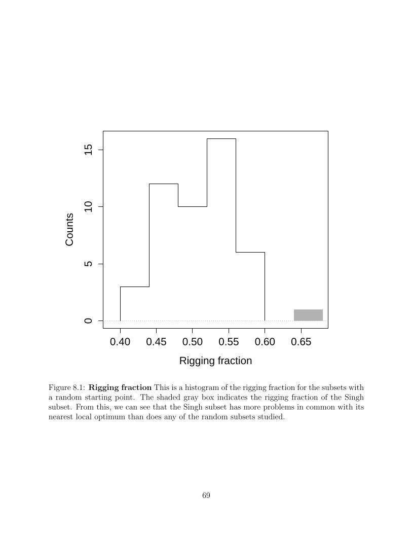
0.40 0.45 0.50 0.55 0.60 0.65
05
1015
Rigging fraction
Cou
nts
Figure 8.1: Rigging fraction This is a histogram of the rigging fraction for the subsets witha random starting point. The shaded gray box indicates the rigging fraction of the Singhsubset. From this, we can see that the Singh subset has more problems in common with itsnearest local optimum than does any of the random subsets studied.
69
Chapter 9
Conclusion
In our endeavor to study the categorization behavior of experts and novices, we have de-
veloped a method for analyzing expert and novice categorizations. In the process, we have
gained insight into different human cognitive structures. Rather than focusing on qualitative
differences in category names, we chose to focus on the groupings of problems. In order to do
this we have created a method for converting an abstract categorization into a graph, which
may then be analyzed. This conversion has laid the foundation for our method of analyzing
card-sorting experiments, which is applicable in any experiment where sorters may put any
single card into more than one category, a behavior which we name multiple categorization.
Using experimental data, we confirmed the null-results that experts and novices are not
distinguishable based on macroscopic features of their card-sorting such as the number of
categories. This held true even when employing graph theoretical approaches. We found
these null results when comparing categorizations’ macroscopic properties, therefore we cre-
ated the Cognitive Categorization Model (CCM), which provided insight into the general
sorter behavior. We found that the best fitting CCM had a multiple categorization prob-
70

ability that depended on the number of categories which led us to determine that sorters
tended toward “stacking” or “spreading” when sorting physics problems. A stacker tended
to create a few general categories and multiply categorize more often. A spreader tended to
create many specific categories and multiply categorize less often. This stacker vs. spreader
behavior is quite independent of the expert vs. novice distinction between our sorters.
As macroscopic properties did not differentiate expert from novice, we studied the mi-
croscopic properties of categorizations by creating and utilizing our distance metric. This
distance metric compares sorters’ categorizations in a manner which takes problem identity
into account. In order to visualize the relative position of our sorters as measured by our
distance metric, we employed Principal Components Analysis. This allowed us to confirm
the stacker vs. spreader distinction as the largest source of variation among sorters. It also
fortuitously found the distinction between experts and novices as the second largest source
of variation.
As was found by Chi et al., we agree that deep structure was an important feature
determining the difference between experts and novices. For this reason it was important to
construct a set of problems from a variety of chapters, our analog for “deep structure”. Yet,
the frequent null results obtained when replicating this experiment, as well as the results
of our own statistical analysis, tell us that we must go beyond chapters and consider the
pedagogical and cognitive properties of the problems that we select. We found that problems
which ask students to perform different procedural tasks (e.g. making a flow chart of how
you would solve a problem) are important to distinguish experts from novices. We also found
that “easy” problems, as determined by a typical introductory physics textbook author, did
a better job of discriminating experts from novices. This is not surprising: a problem is so
71
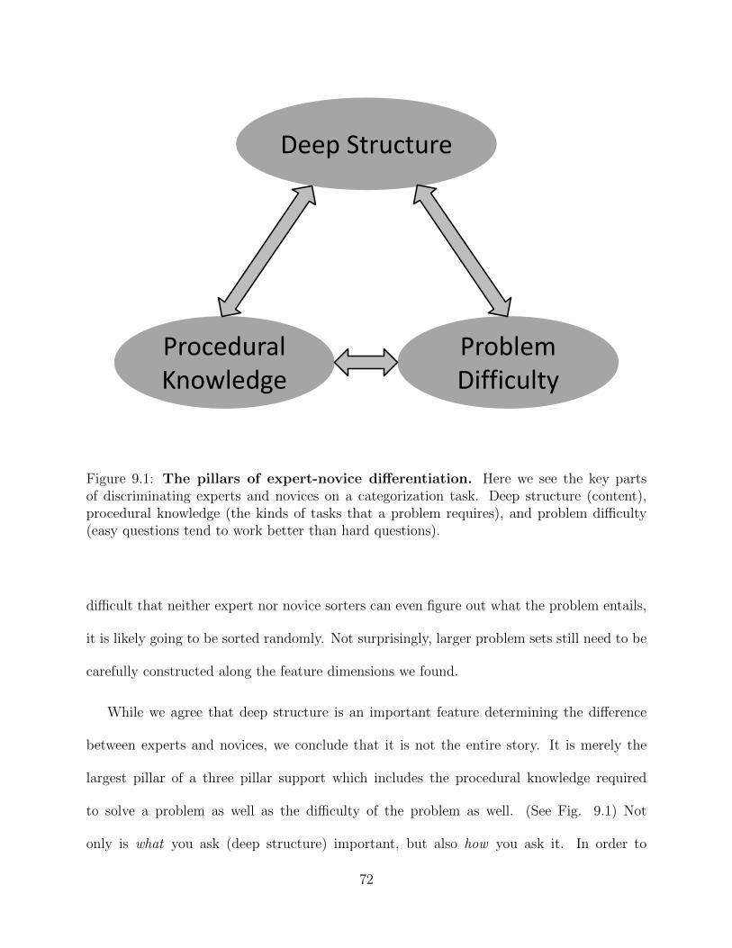
Deep Structure
Procedural Knowledge
Problem Difficulty
Figure 9.1: The pillars of expert-novice differentiation. Here we see the key partsof discriminating experts and novices on a categorization task. Deep structure (content),procedural knowledge (the kinds of tasks that a problem requires), and problem difficulty(easy questions tend to work better than hard questions).
difficult that neither expert nor novice sorters can even figure out what the problem entails,
it is likely going to be sorted randomly. Not surprisingly, larger problem sets still need to be
carefully constructed along the feature dimensions we found.
While we agree that deep structure is an important feature determining the difference
between experts and novices, we conclude that it is not the entire story. It is merely the
largest pillar of a three pillar support which includes the procedural knowledge required
to solve a problem as well as the difficulty of the problem as well. (See Fig. 9.1) Not
only is what you ask (deep structure) important, but also how you ask it. In order to
72

differentiate experts from novices on a categorization task we also need to ask questions
which require different procedural tasks (e.g. make a flow chart). One might have hoped
that these experiments would most strongly identify experts based on the types of declarative
knowledge and procedural knowledge instead, which are arguably more authentic indicators
of expert-likeness in real life. However, the relegation of deep structure from its former
lonesome perch as the single salient feature which discriminates experts from novices to part
of this triad is still a satisfying result which reflects the understanding gained since Chi et al.
published their seminal result.
9.1 Outlook
Even after considering all feature dimensions in this study, only 42.7% of the variability in
the 10-problem set was explained. This means that there may be other latent variables,
perhaps closely linked to the surface features in each problem, need to be considered. In
other words, the remaining variability can possibly only be resolved by intentionally planting
surface features, as in Veldhuis’ study [2]. Also, we need to understand the process of sorting,
not just the outcome. The first step in understanding the process was the development of the
CCM. However, as this model is only intended to describe the macroscopic sorting behavior,
it is “blind” to the problems, e.g., it cannot even begin to simulate the sorters’ reactions to
different features of the individual problems.
Likely the only way to gain a better understand of the sorting process will be to deploy
a “think-aloud” protocol, where sorters are asked to talk us through their sorting decisions.
Combining the ideas gleaned from a think-aloud protocol with a model which can describe the
internal cognitive process of categorization will be the key to understanding this outstand-
73

ing variability and predicting an instrument’s ability to discriminate experts from novices.
Ultimately, the goal would be to simulate the process of categorization.
74

APPENDICES
75

Appendix A
Categorization Model Pseudocode
As stated earlier, the purpose of the Cognitive Categorization Model was to account for the
common macroscopic sorting behavior of experts and novices. In order to do this, we created
a statistical model which attempted to model the sorting process. We assumed that there
were three rules to this sorting process:
1. All questions must be put into a category
2. All categories must have at least one question in them
3. A question may fall into one category
Once we assumed these three rules, we created a model which has three input parameters:
1. The number of questions (which is fixed by the experiment)
2. The average number of categories for all sorters
3. The multiple categorization parameterization
76
We fixed the number of questions and optimized the other parameters so that the model
would capture the sorters’ macroscopic behavior. By only having two free parameters, we
know that we have created a model which parsimoniously describes the sorter behavior rather
than soaking up statistical variation by over-fitting it.
A.1 Pseudocode
The following pseudocode creates a weighted adjacency matrix for a random categorization
according to our best-fitting categorization model. This matrix may then be used to create
a graph. Increasing the utility of the weighted adjacency matrix is the fact that many graph
theory statistics are calculated using the weighted adjacency matrix or the adjacency matrix
(which is a boolean version of the weighted adjacency matrix).
for each graph
Q = input parameter # number of questions
beta = input parameter # multiple categorization param.
Cbar = input parameter # avg. number of categories
# Pick the number of categories from the proper distribution.
C = 1 + random deviation from binomial
# Binomial properties: num. trials = Q-1 and avg = Cbar-1
Pmult = betaC # multiple sorting probability for CCMv3
# Create boolean T matrix; rows are questions columns are categories
Initialize T
X = shuffle question numbers
Y = shuffle list of category numbers from 1 to C
77
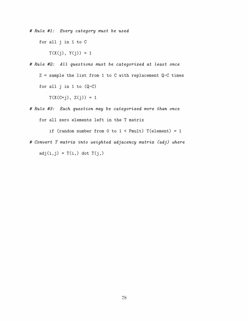
# Rule #1: Every category must be used
for all j in 1 to C
T(X(j), Y(j)) = 1
# Rule #2: All questions must be categorized at least once
Z = sample the list from 1 to C with replacement Q-C times
for all j in 1 to (Q-C)
T(X(C+j), Z(j)) = 1
# Rule #3: Each question may be categorized more than once
for all zero elements left in the T matrix
if (random number from 0 to 1 < Pmult) T(element) = 1
# Convert T matrix into weighted adjacency matrix (adj) where
adj(i,j) = T(i,) dot T(j,)
78

Appendix B
Distance metric
The following distance metric quantifies the number of edges that must be added or removed
from a graph to make it identical to another graph:
drs =1
2
Q∑i=1
Q∑j=1
∣∣∣Xrij −Xsij∣∣∣ (B.1)
Where Xrij is the (i, j)th element in the weighted adjacency matrix for reviewer r. The
properties of a metric are as follows:
drs ≥ 0
drs = 0 ⇐⇒ Xr = Xs
drs = dsr
drt ≤ drs + dst (B.2)
79
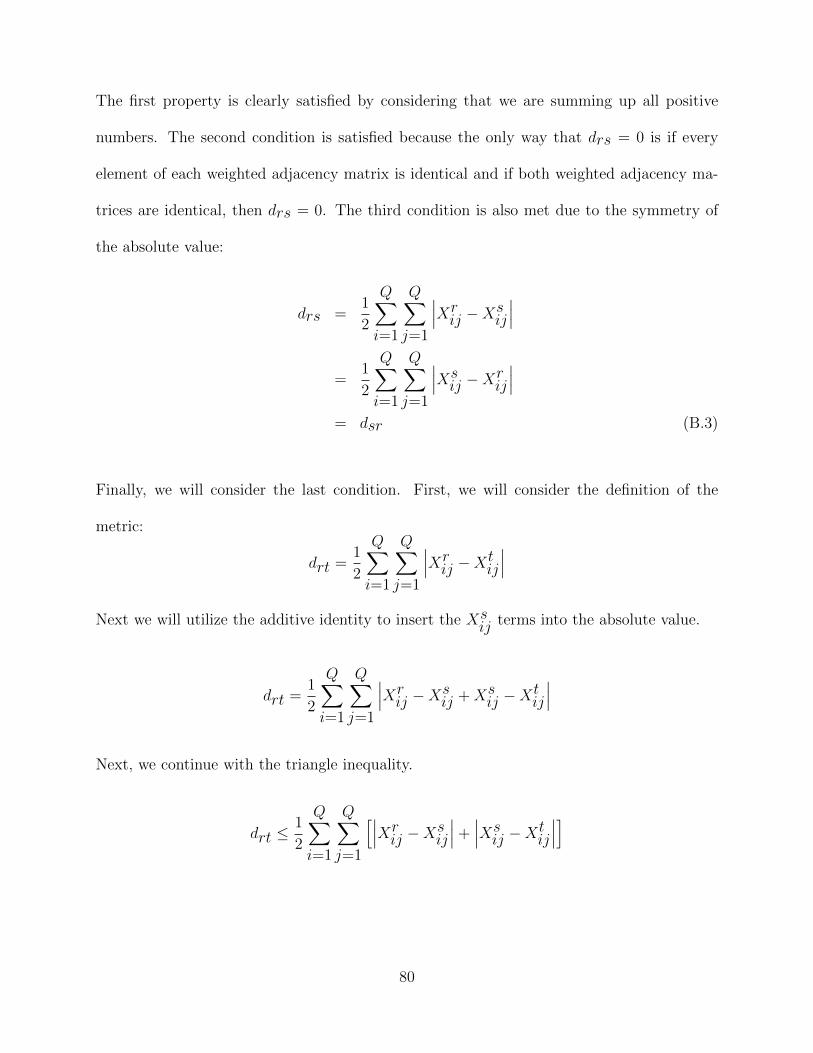
The first property is clearly satisfied by considering that we are summing up all positive
numbers. The second condition is satisfied because the only way that drs = 0 is if every
element of each weighted adjacency matrix is identical and if both weighted adjacency ma-
trices are identical, then drs = 0. The third condition is also met due to the symmetry of
the absolute value:
drs =1
2
Q∑i=1
Q∑j=1
∣∣∣Xrij −Xsij∣∣∣=
1
2
Q∑i=1
Q∑j=1
∣∣∣Xsij −Xrij∣∣∣= dsr (B.3)
Finally, we will consider the last condition. First, we will consider the definition of the
metric:
drt =1
2
Q∑i=1
Q∑j=1
∣∣∣Xrij −Xtij∣∣∣Next we will utilize the additive identity to insert the Xsij terms into the absolute value.
drt =1
2
Q∑i=1
Q∑j=1
∣∣∣Xrij −Xsij +Xsij −Xtij
∣∣∣Next, we continue with the triangle inequality.
drt ≤1
2
Q∑i=1
Q∑j=1
[∣∣∣Xrij −Xsij∣∣∣+∣∣∣Xsij −Xtij∣∣∣]
80

Now we distribute the term in front of the sum.
drt ≤
1
2
Q∑i=1
Q∑j=1
∣∣∣Xrij −Xsij∣∣∣+
1
2
Q∑i=1
Q∑j=1
∣∣∣Xsij −Xtij∣∣∣
And then we simplify using the definition of our metric.
drt ≤ drs + dst (B.4)
So we have shown that this is a metric.
B.1 Pseudocode
This pseudocode function will compute the distance between two sorters with known weighted
adjacency matrices wadj1 and wadj2.
dmetric = function(wadj1,wadj2)
Make sure each matrix is square and has same dimensions
diff = abs(wadj1 - wadj2)
dist = 0.5*sum(diff)
return(dist)
The distance matrix is then calculated by applying the dmetric function on each pair of
sorters’ weighted adjacency matricies.
81
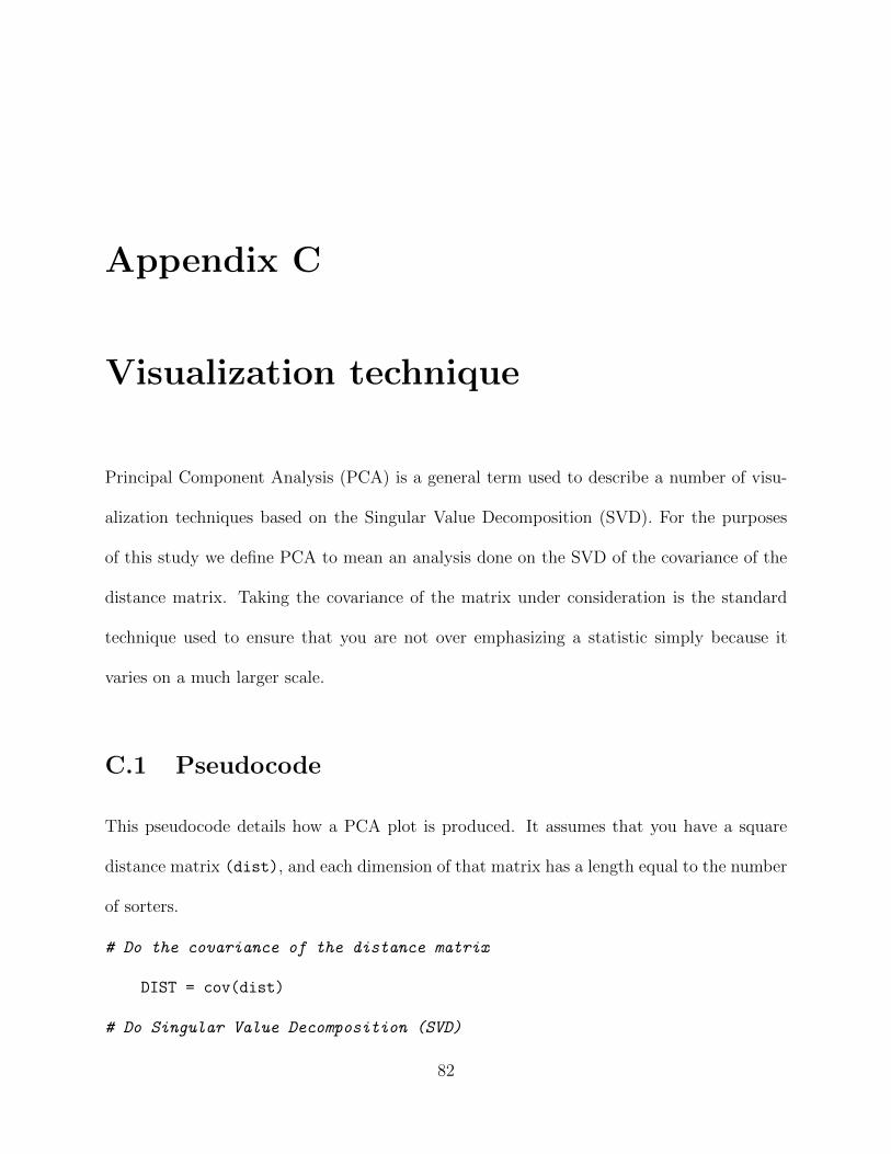
Appendix C
Visualization technique
Principal Component Analysis (PCA) is a general term used to describe a number of visu-
alization techniques based on the Singular Value Decomposition (SVD). For the purposes
of this study we define PCA to mean an analysis done on the SVD of the covariance of the
distance matrix. Taking the covariance of the matrix under consideration is the standard
technique used to ensure that you are not over emphasizing a statistic simply because it
varies on a much larger scale.
C.1 Pseudocode
This pseudocode details how a PCA plot is produced. It assumes that you have a square
distance matrix (dist), and each dimension of that matrix has a length equal to the number
of sorters.
# Do the covariance of the distance matrix
DIST = cov(dist)
# Do Singular Value Decomposition (SVD)
82

dist.svd = svd(DIST)
# Look at eigenvectors of the SVD
evector1 = dist.svd.U[1]
evector2 = dist.svd.U[2]
# More eigenvectors allow you to study more dimensions of the PCA
# Calculate principal components:
pc1 = dist × evector1
pc2 = dist × evector2
# Note: × indicates matrix multiplication
plot(pc1,pc2)
83
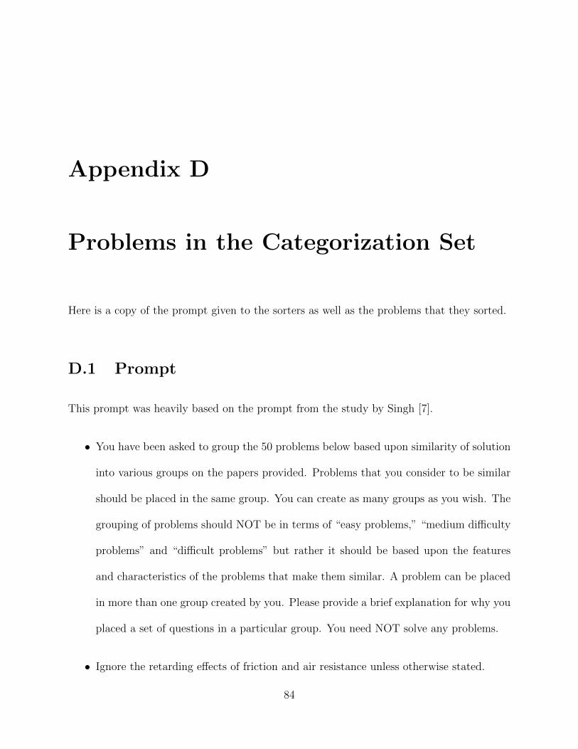
Appendix D
Problems in the Categorization Set
Here is a copy of the prompt given to the sorters as well as the problems that they sorted.
D.1 Prompt
This prompt was heavily based on the prompt from the study by Singh [7].
• You have been asked to group the 50 problems below based upon similarity of solution
into various groups on the papers provided. Problems that you consider to be similar
should be placed in the same group. You can create as many groups as you wish. The
grouping of problems should NOT be in terms of “easy problems,” “medium difficulty
problems” and “difficult problems” but rather it should be based upon the features
and characteristics of the problems that make them similar. A problem can be placed
in more than one group created by you. Please provide a brief explanation for why you
placed a set of questions in a particular group. You need NOT solve any problems.
• Ignore the retarding effects of friction and air resistance unless otherwise stated.
84
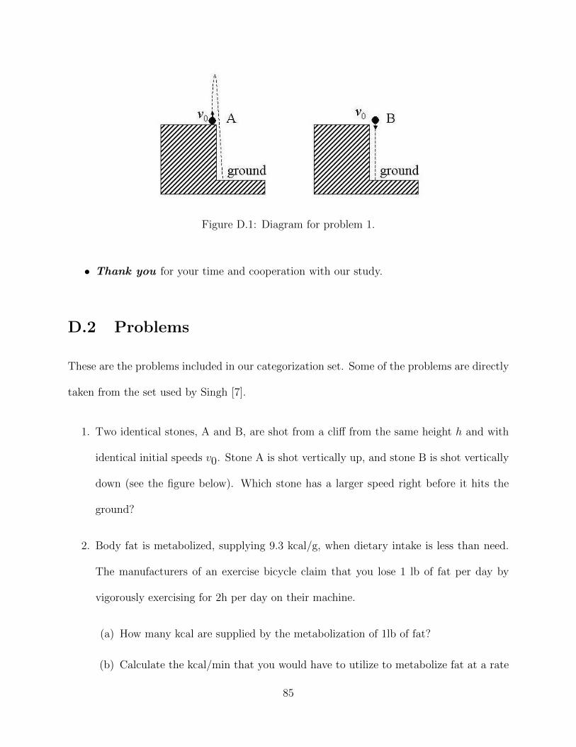
Figure D.1: Diagram for problem 1.
• Thank you for your time and cooperation with our study.
D.2 Problems
These are the problems included in our categorization set. Some of the problems are directly
taken from the set used by Singh [7].
1. Two identical stones, A and B, are shot from a cliff from the same height h and with
identical initial speeds v0. Stone A is shot vertically up, and stone B is shot vertically
down (see the figure below). Which stone has a larger speed right before it hits the
ground?
2. Body fat is metabolized, supplying 9.3 kcal/g, when dietary intake is less than need.
The manufacturers of an exercise bicycle claim that you lose 1 lb of fat per day by
vigorously exercising for 2h per day on their machine.
(a) How many kcal are supplied by the metabolization of 1lb of fat?
(b) Calculate the kcal/min that you would have to utilize to metabolize fat at a rate
85
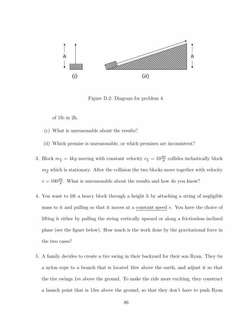
Figure D.2: Diagram for problem 4.
of 1lb in 2h.
(c) What is unreasonable about the results?
(d) Which premise is unreasonable, or which premises are inconsistent?
3. Block m1 = 4kg moving with constant velocity v1 = 10ms collides inelastically block
m2 which is stationary. After the collision the two blocks move together with velocity
v = 100ms . What is unreasonable about the results and how do you know?
4. You want to lift a heavy block through a height h by attaching a string of negligible
mass to it and pulling so that it moves at a constant speed v. You have the choice of
lifting it either by pulling the string vertically upward or along a frictionless inclined
plane (see the figure below). How much is the work done by the gravitational force in
the two cases?
5. A family decides to create a tire swing in their backyard for their son Ryan. They tie
a nylon rope to a branch that is located 16m above the earth, and adjust it so that
the tire swings 1m above the ground. To make the ride more exciting, they construct
a launch point that is 13m above the ground, so that they don’t have to push Ryan
86
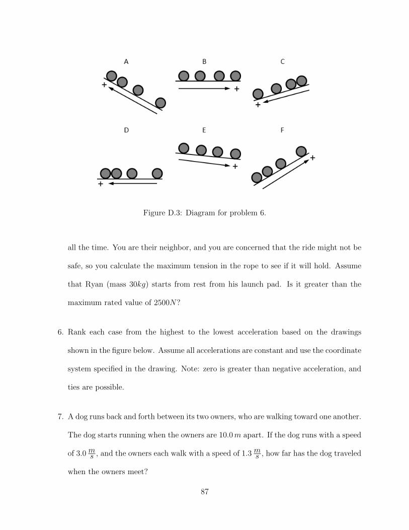
Figure D.3: Diagram for problem 6.
all the time. You are their neighbor, and you are concerned that the ride might not be
safe, so you calculate the maximum tension in the rope to see if it will hold. Assume
that Ryan (mass 30kg) starts from rest from his launch pad. Is it greater than the
maximum rated value of 2500N?
6. Rank each case from the highest to the lowest acceleration based on the drawings
shown in the figure below. Assume all accelerations are constant and use the coordinate
system specified in the drawing. Note: zero is greater than negative acceleration, and
ties are possible.
7. A dog runs back and forth between its two owners, who are walking toward one another.
The dog starts running when the owners are 10.0m apart. If the dog runs with a speed
of 3.0 ms , and the owners each walk with a speed of 1.3 ms , how far has the dog traveled
when the owners meet?
87
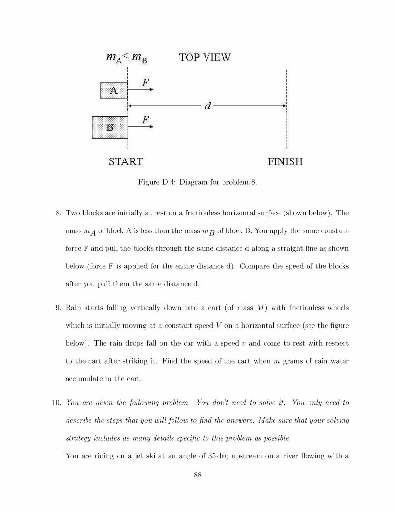
Figure D.4: Diagram for problem 8.
8. Two blocks are initially at rest on a frictionless horizontal surface (shown below). The
mass mA of block A is less than the mass mB of block B. You apply the same constant
force F and pull the blocks through the same distance d along a straight line as shown
below (force F is applied for the entire distance d). Compare the speed of the blocks
after you pull them the same distance d.
9. Rain starts falling vertically down into a cart (of mass M) with frictionless wheels
which is initially moving at a constant speed V on a horizontal surface (see the figure
below). The rain drops fall on the car with a speed v and come to rest with respect
to the cart after striking it. Find the speed of the cart when m grams of rain water
accumulate in the cart.
10. You are given the following problem. You don’t need to solve it. You only need to
describe the steps that you will follow to find the answers. Make sure that your solving
strategy includes as many details specific to this problem as possible.
You are riding on a jet ski at an angle of 35 deg upstream on a river flowing with a
88

Figure D.5: Diagram for problem 9.
speed of 2.8 ms . If your velocity relative to the ground is 9.5 ms at an angle of 20.0 deg
upstream, what is the speed of the jet ski relative to the water?
11. A force of 9.4N pulls horizontally on a 1.1 kg block that slides on a rough, horizontal
surface. This block is connected by a horizontal string to a second block of mass
m2 = 1.92 kg on the same surface. The coefficient of kinetic friction is µk = 0.24 for
both blocks. What is the acceleration of the blocks?
12. Three blocks (m1 = 1kg, m2 = 2kg, m3 = 3kg) are in a straight line in contact with
each other on a frictionless horizontal table (block with mass m2 is in the middle). A
constant horizontal force FH = 3N is applied to the block with mass m1. Find the
forces exerted on m1 by m2 and on m2 by m3.
13. The figure below shows two blocks on a frictionless inclined plane with an angle of
inclination θ = 40 deg and the two connected to each other via a massless rope. The
rope that connects the two blocks goes around a frictionless, massless pulley and is
89
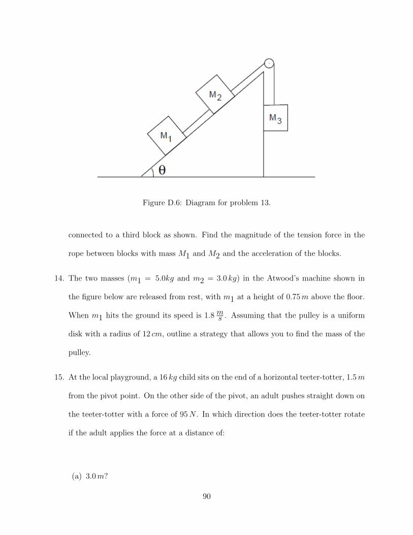
Figure D.6: Diagram for problem 13.
connected to a third block as shown. Find the magnitude of the tension force in the
rope between blocks with mass M1 and M2 and the acceleration of the blocks.
14. The two masses (m1 = 5.0kg and m2 = 3.0 kg) in the Atwood’s machine shown in
the figure below are released from rest, with m1 at a height of 0.75m above the floor.
When m1 hits the ground its speed is 1.8 ms . Assuming that the pulley is a uniform
disk with a radius of 12 cm, outline a strategy that allows you to find the mass of the
pulley.
15. At the local playground, a 16 kg child sits on the end of a horizontal teeter-totter, 1.5m
from the pivot point. On the other side of the pivot, an adult pushes straight down on
the teeter-totter with a force of 95N . In which direction does the teeter-totter rotate
if the adult applies the force at a distance of:
(a) 3.0m?
90
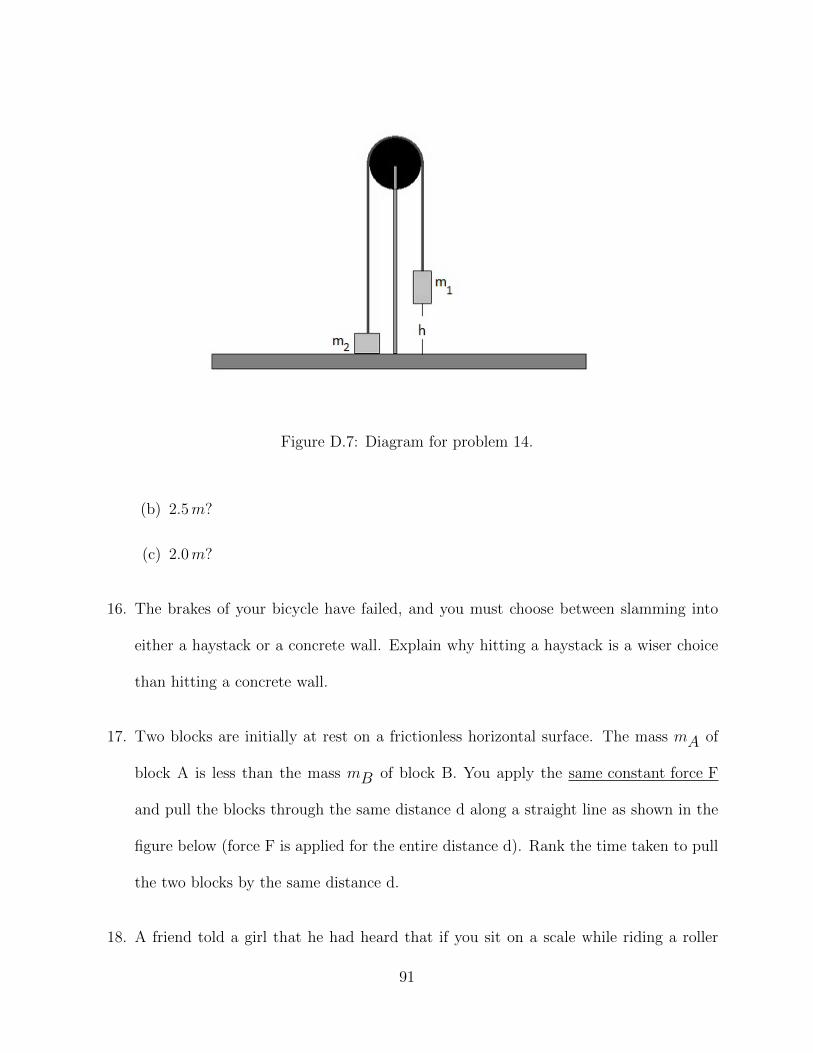
Figure D.7: Diagram for problem 14.
(b) 2.5m?
(c) 2.0m?
16. The brakes of your bicycle have failed, and you must choose between slamming into
either a haystack or a concrete wall. Explain why hitting a haystack is a wiser choice
than hitting a concrete wall.
17. Two blocks are initially at rest on a frictionless horizontal surface. The mass mA of
block A is less than the mass mB of block B. You apply the same constant force F
and pull the blocks through the same distance d along a straight line as shown in the
figure below (force F is applied for the entire distance d). Rank the time taken to pull
the two blocks by the same distance d.
18. A friend told a girl that he had heard that if you sit on a scale while riding a roller
91
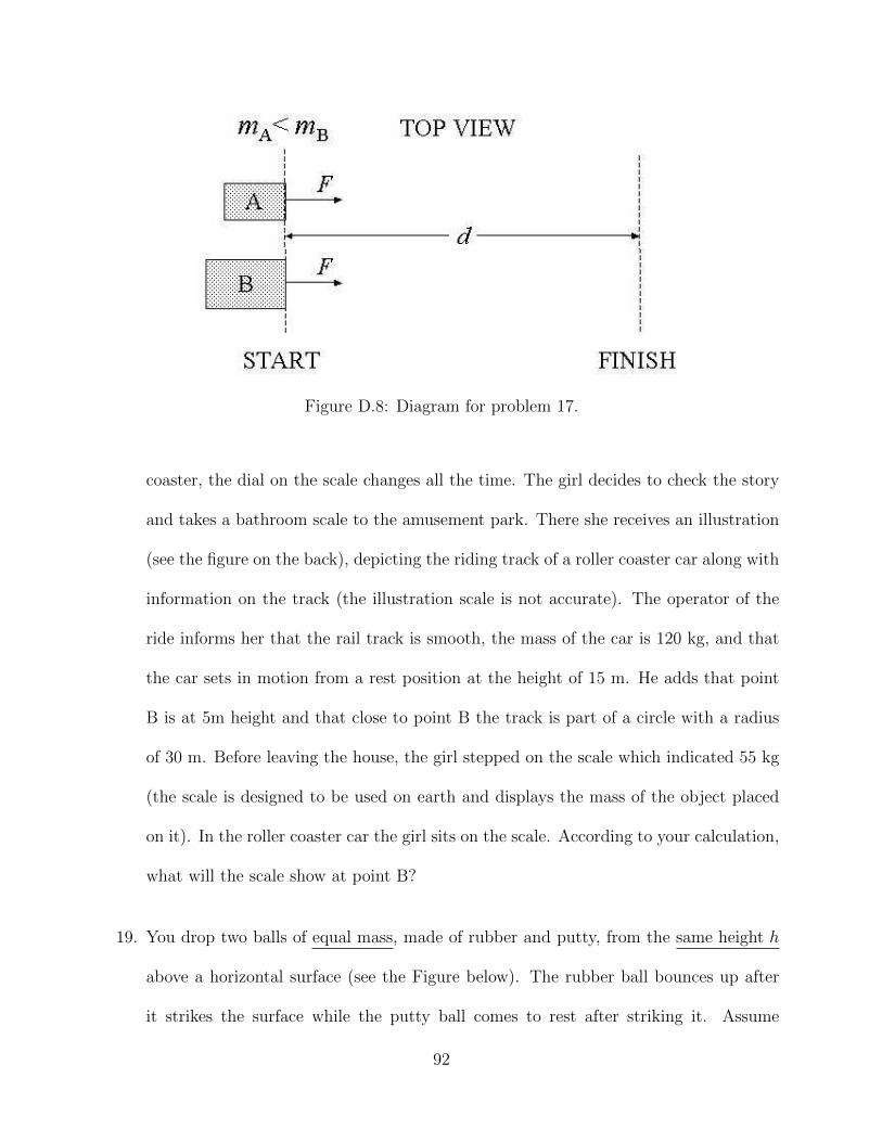
Figure D.8: Diagram for problem 17.
coaster, the dial on the scale changes all the time. The girl decides to check the story
and takes a bathroom scale to the amusement park. There she receives an illustration
(see the figure on the back), depicting the riding track of a roller coaster car along with
information on the track (the illustration scale is not accurate). The operator of the
ride informs her that the rail track is smooth, the mass of the car is 120 kg, and that
the car sets in motion from a rest position at the height of 15 m. He adds that point
B is at 5m height and that close to point B the track is part of a circle with a radius
of 30 m. Before leaving the house, the girl stepped on the scale which indicated 55 kg
(the scale is designed to be used on earth and displays the mass of the object placed
on it). In the roller coaster car the girl sits on the scale. According to your calculation,
what will the scale show at point B?
19. You drop two balls of equal mass, made of rubber and putty, from the same height h
above a horizontal surface (see the Figure below). The rubber ball bounces up after
it strikes the surface while the putty ball comes to rest after striking it. Assume
92
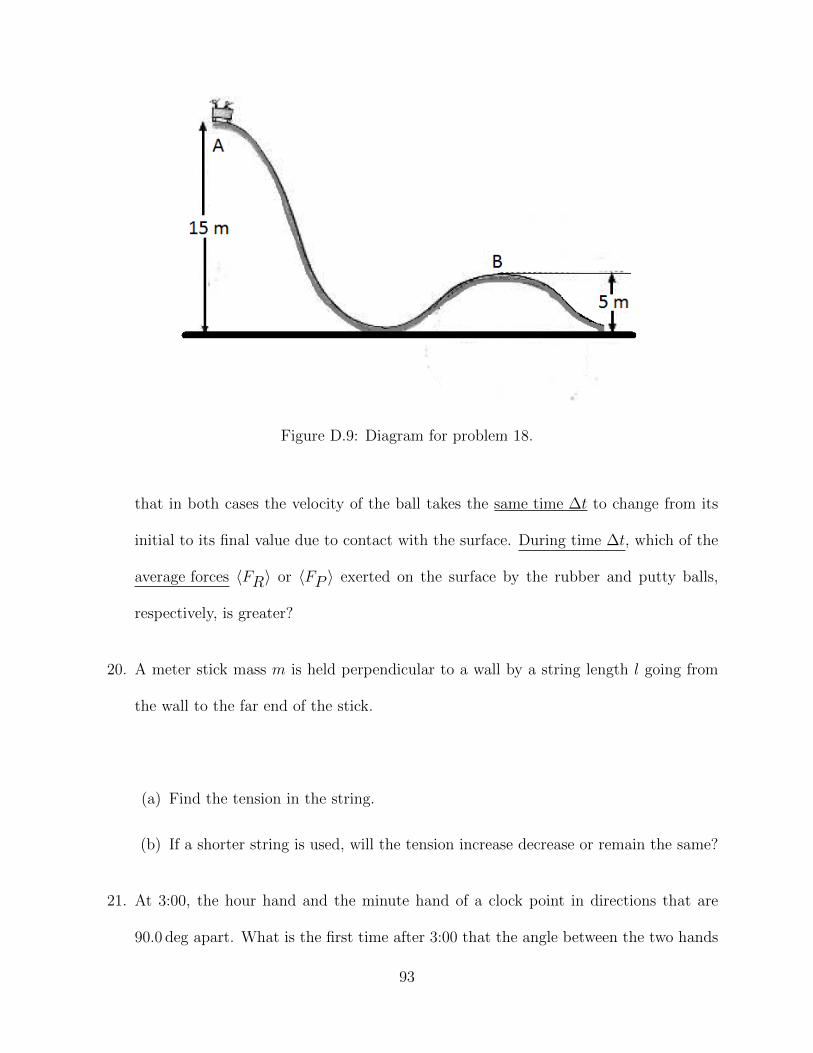
Figure D.9: Diagram for problem 18.
that in both cases the velocity of the ball takes the same time ∆t to change from its
initial to its final value due to contact with the surface. During time ∆t, which of the
average forces 〈FR〉 or 〈FP 〉 exerted on the surface by the rubber and putty balls,
respectively, is greater?
20. A meter stick mass m is held perpendicular to a wall by a string length l going from
the wall to the far end of the stick.
(a) Find the tension in the string.
(b) If a shorter string is used, will the tension increase decrease or remain the same?
21. At 3:00, the hour hand and the minute hand of a clock point in directions that are
90.0 deg apart. What is the first time after 3:00 that the angle between the two hands
93

Figure D.10: Diagram for problem 19.
has decreased to 45.0 deg?
22. A cyclist approaches the bottom of a gradual hill at a speed of 15ms . The hill is 5m
high, and the cyclist estimates that she is going fast enough to coast up and over it
without peddling. Ignoring friction and air resistance, find the speed at which the
cyclist crests the hill? Neglect the kinetic energy of the rotating wheels.
23. Two identical stones, A and B, are shot from a cliff from the same height h and with
identical initial speeds v0. Stone A is shot at an angle of 30 deg above the horizontal
and stone B is shot at an angle of 30 deg below the horizontal. Which stone takes a
longer time to hit the ground?
24. You are given the following problem. You don’t need to solve it. You only need to
create a flow chart to illustrate the steps you are going to follow to find the answers.
Make sure that your solving strategy includes as many details specific to this problem
as possible.
The press box at a baseball park is 38.0 ft above the ground. A reporter in the press
box looks at an angle of 15.0 deg below the horizontal to see second base. What is the
94

horizontal distance from the press box to second base?
25. You are given the following problem. You don’t need to solve it. You only need to
create a flow chart to illustrate the steps you are going to follow to find the answers.
Make sure that your solving strategy includes as many details specific to this problem
as possible.
The coefficient of static friction between a block and a horizontal floor is 0.35, while
the coefficient of kinetic friction is 0.22. The mass of the block is 4.6 kg and it is
initially at rest. Once the block is sliding, if you keep pushing on it with the same
minimum starting force as in part a), does the block move with constant velocity or
does it accelerate?
26. You are given the following problem. You don’t need to solve it. You only need to
create a flow chart to illustrate the steps you are going to follow to find the answers.
Make sure that your solving strategy includes as many details specific to this problem
as possible.
Harry Potter and Voldemort are wrestling inside a cart traveling east at a speed of
45ms directly toward an abyss. Harry then notices the danger and jumps backward due
west off of the cart. Ron who stands on safe ground in the back notices that Harry’s
velocity due west at the jump is 15ms relative to the ground. What is the speed of the
cart after Harry jumps off of it? The mass of the cart is 200kg, Harry’s mass is 60kg,
and Voldemort’s mass is 80kg.
27. In the figure below, a horizontal spring with spring constant k1 = 8Nm is compressed
20cm from its equilibrium position by a 4kg block. Then, the block is released. What
would be the maximum compression of a spring (k2 = 5Nm ) on the inclined plane when
95
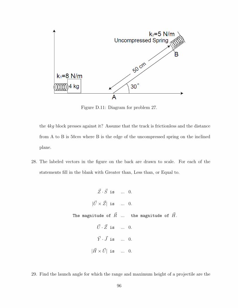
Figure D.11: Diagram for problem 27.
the 4kg block presses against it? Assume that the track is frictionless and the distance
from A to B is 50cm where B is the edge of the uncompressed spring on the inclined
plane.
28. The labeled vectors in the figure on the back are drawn to scale. For each of the
statements fill in the blank with Greater than, Less than, or Equal to.
~Z · ~S is ... 0.
|~U × ~Z| is ... 0.
The magnitude of ~R ... the magnitude of ~H.
~U · ~Z is ... 0.
~Y · ~J is ... 0.
| ~H × ~U | is ... 0.
29. Find the launch angle for which the range and maximum height of a projectile are the
96
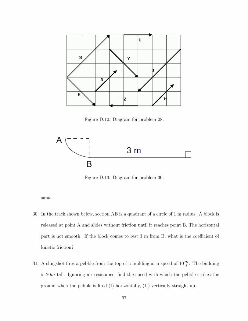
Figure D.12: Diagram for problem 28.
Figure D.13: Diagram for problem 30.
same.
30. In the track shown below, section AB is a quadrant of a circle of 1 m radius. A block is
released at point A and slides without friction until it reaches point B. The horizontal
part is not smooth. If the block comes to rest 3 m from B, what is the coefficient of
kinetic friction?
31. A slingshot fires a pebble from the top of a building at a speed of 10ms . The building
is 20m tall. Ignoring air resistance, find the speed with which the pebble strikes the
ground when the pebble is fired (I) horizontally, (II) vertically straight up.
97
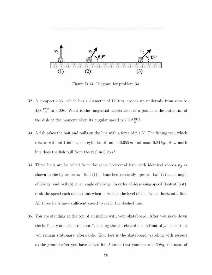
Figure D.14: Diagram for problem 34.
32. A compact disk, which has a diameter of 12.0cm, speeds up uniformly from zero to
4.00revs in 3.00s. What is the tangential acceleration of a point on the outer rim of
the disk at the moment when its angular speed is 2.00revs ?
33. A fish takes the bait and pulls on the line with a force of 2.1N . The fishing reel, which
rotates without friction, is a cylinder of radius 0.055m and mass 0.84 kg. How much
line does the fish pull from the reel in 0.25 s?
34. Three balls are launched from the same horizontal level with identical speeds v0 as
shown in the figure below. Ball (1) is launched vertically upward, ball (2) at an angle
of 60 deg, and ball (3) at an angle of 45 deg. In order of decreasing speed (fastest first),
rank the speed each one attains when it reaches the level of the dashed horizontal line.
All three balls have sufficient speed to reach the dashed line.
35. You are standing at the top of an incline with your skateboard. After you skate down
the incline, you decide to “abort”, kicking the skateboard out in front of you such that
you remain stationary afterwards. How fast is the skateboard traveling with respect
to the ground after you have kicked it? Assume that your mass is 60kg, the mass of
98

the skateboard is 10kg, and the height of the incline is 10cm.
36. Two frictionless inclined planes have the same height but have different angles of incli-
nations of 45 deg and 60 deg with respect to the horizontal. You slide down from the
top which is at a height h above the ground on each inclined planes starting from rest.
Find the time taken to reach the bottom in the two cases.
37. A turntable with a moment of inertia of 5.4×10⁻³kg m2 rotates freely with an angular
speed of 33 13 rpm. Riding on the rim of the turntable, 15 cm from the center, is a 1.3 g
cricket. If the cricket walks to the center of the turntable, will the turntable rotate
faster, slower, or at the same rate? Explain.
38. A 2.0 kg solid sphere (radius = 0.10m) is released from rest at the top of a ramp and
allowed to roll without slipping. The ramp is 0.75m high and 5.0m long. When the
sphere reaches the bottom of the ramp, what is
(a) its total kinetic energy?
(b) its rotational kinetic energy?
(c) its translational kinetic energy?
39. Two frictionless inclined planes have the same height but have different angles of incli-
nations of 45 deg and 60 deg with respect to the horizontal. You slide down from the
top which is at a height h above the ground on each inclined planes starting from rest.
Find your speed at the bottom of the inclined planes in the two cases.
40. A ball is thrown from the top of a 35m high building with an initial speed of 80ms at
99
an angle of 25 deg above the horizontal. Find the time it takes to reach the ground.
41. On October 9, 1992, a 27 pound meteorite struck a car in Peekskill, NY, creating a
dent about 22 cm deep. If the initial speed of the meteorite was 550 ms , what was the
average force exerted on the meteorite by the car?
42. The corners of a square with sides 2.5m long lie on a circle. Is the radius of the circle
greater than, less than, or equal to the length of a side of the square? Explain.
43. At amusement parks, there is a popular ride in which the floor of a rotating cylindrical
room falls away, leaving the backs of the riders “plastered” against the wall. Suppose
the radius of the room is 3.3 m and the speed of the wall is 10ms when the floor falls
away. What is the minimum coefficient of friction that must exist between a rider’s
back and the wall, if the rider is to remain in place when the floor drops away?
44. Your friend Dan, who is in a ski resort, competes with his twin brother Sam on who can
glide higher with the snowboard. Sam, whose mass is 60 kg, puts his 15 kg snowboard
on a level section of the track, 5 meters from a slope (inclined plane). Then, Sam takes
a running start and jumps onto the stationary snowboard. Sam and the snowboard
glide together till they come to rest at a height of 1.8 m above the starting level. What
is the minimum speed at which Dan should run to glide higher than his brother to
win the competition? Dan has the same weight as Sam and his snowboard weighs the
same as Sam’s snowboard.
45. Legend has it that Isaac Newton was hit on the head by a falling apple, thus triggering
his thoughts on gravity. Assuming the story to be true, estimate the speed of the apple
when it struck Newton.
100

46. An astronaut is floating next a space shuttle out in the middle of the intergalactic void
(i.e. very far from the influence of any planets or stars). Consider the astronaut and
the shuttle to be an isolated system. The astronaut accidentally kicks the shuttle with
his feet. Which of the following statements are true?
• The astronaut can never get back to the shuttle because once you have a certain
momentum it cannot be changed.
• The shuttle and the astronaut move apart from each other with the astronaut’s
velocity being larger than the shuttle’s velocity.
• The momentum of the shuttle is smaller than the momentum of the astronaut.
• In order to get back to the shuttle, the astronaut needs a change in momentum.
• The total momentum of the astronaut-shuttle system might not be conserved,
depending on how hard the shuttle was kicked.
47. Two small spheres of putty, A and B, of equal mass, hang from the ceiling on massless
strings of equal length. Sphere A is raised to a height h0 as shown in the figure below
and released. It collides with sphere B (which is initially at rest); they stick and swing
together to a maximum height hf . Find the height hf in terms of h0.
48. A kayaker paddles with a power output of 50.0W to maintain a speed of 1.50ms .
(a) Calculate the resistive force exerted by the water on the kayak.
(b) If the kayaker doubles her power output, and the resistive force due to the water
remains the same, by what factor does the kayaker’s speed change?
49. You are given the following problem. You don’t need to solve it. You only need to
101
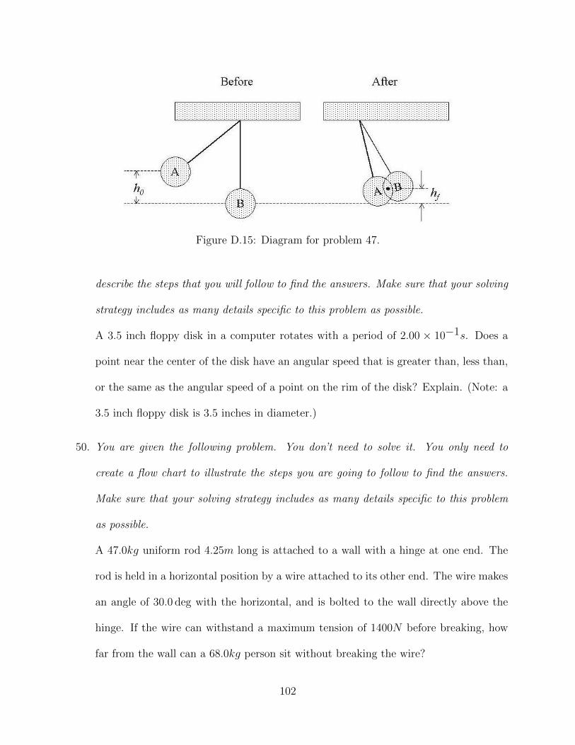
Figure D.15: Diagram for problem 47.
describe the steps that you will follow to find the answers. Make sure that your solving
strategy includes as many details specific to this problem as possible.
A 3.5 inch floppy disk in a computer rotates with a period of 2.00 × 10⁻¹s. Does a
point near the center of the disk have an angular speed that is greater than, less than,
or the same as the angular speed of a point on the rim of the disk? Explain. (Note: a
3.5 inch floppy disk is 3.5 inches in diameter.)
50. You are given the following problem. You don’t need to solve it. You only need to
create a flow chart to illustrate the steps you are going to follow to find the answers.
Make sure that your solving strategy includes as many details specific to this problem
as possible.
A 47.0kg uniform rod 4.25m long is attached to a wall with a hinge at one end. The
rod is held in a horizontal position by a wire attached to its other end. The wire makes
an angle of 30.0 deg with the horizontal, and is bolted to the wall directly above the
hinge. If the wire can withstand a maximum tension of 1400N before breaking, how
far from the wall can a 68.0kg person sit without breaking the wire?
102
Appendix E
Sorter Graphs
Included here are the graphs of the sorters from our study. Sorters 1-18 are experts and
Sorters 19-41 are novices. Each vertex represents a problem, and is labeled by the problem
number in our study. The edges are drawn between problems in the same category. Vertex
placement has been done using the Fruchterman-Reingold algorithm [27] as it did the best
job of displaying multiple categorization. Categories tend to form in large “ball” shapes.
Multiple categorization is evident by the appearance of an “arm” out of one of the categories.
103
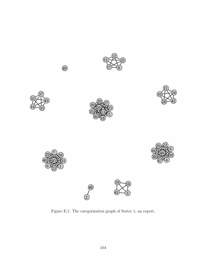
●
●●
●
●
●
●
●
●
●
●●
●● ●
●
●
●
●
●
●
●
●
●
●
●
● ●
● ●●
●
●
●
●●
●
●
●
●
●
●●
●
●●
●
●
●
●
1
23
4
5
6
7
8
9
10
1112
1314 15
16
17
18
19
20
21
22
23
24
25
26
27 28
29 30
31
32
33
34
3536
37
38
39
40
41
4243
44
45
46
47
48
49
50
Figure E.1: The categorization graph of Sorter 1, an expert.
104
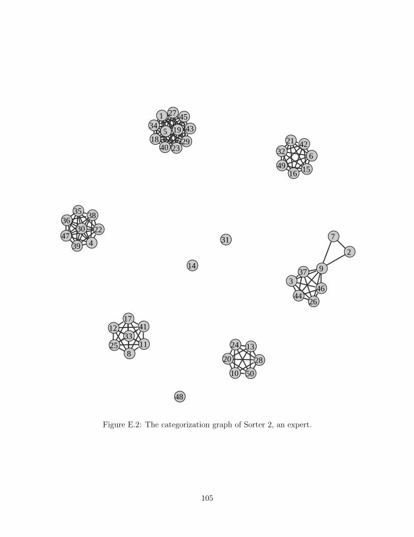
●
●
●
●
●
●
●
●
●
●
●●
●
●
●●
●
●●
●
●
●
●
●●
●
●
●
●
●●
●
●
●
●●
●
●
●
●
●
●●
●
●
●
●
●
●
●
1
2
3
4
5
6
7
8
9
10
11
12
13
14
1516
17
1819
20
21
22
23
2425
26
27
28
29
3031
32
33
34
3536
37
38
39
40
41
42
43
44
45
46
47
48
49
50
Figure E.2: The categorization graph of Sorter 2, an expert.
105
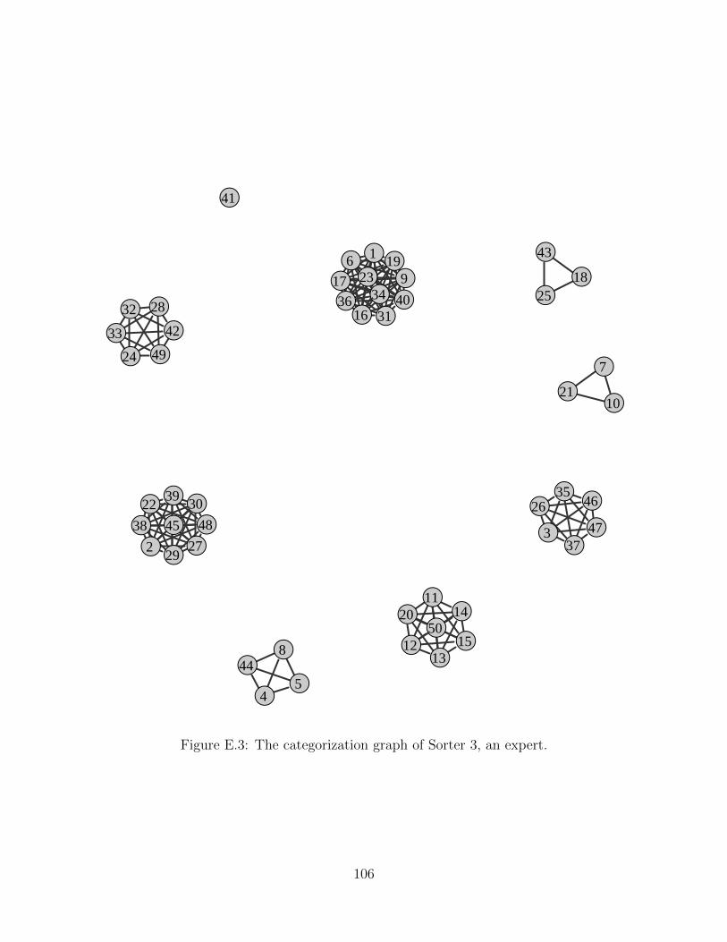
●
●●
●●
●
●
●
●
●
●
●●
●
●
●
● ●●
●
●
●
●
●
●
●
●
●
●
●
●●●
●
●
●
●●
●
●
●
●
●
●
●●●●
●
●
1
23
45
6
7
8
9
10
11
1213
14
15
16
17 1819
20
21
22
23
24
25
26
27
28
29
30
3132
33
34
35
36
3738
39
40
41
42
43
44
45
46
4748
49
50
Figure E.3: The categorization graph of Sorter 3, an expert.
106
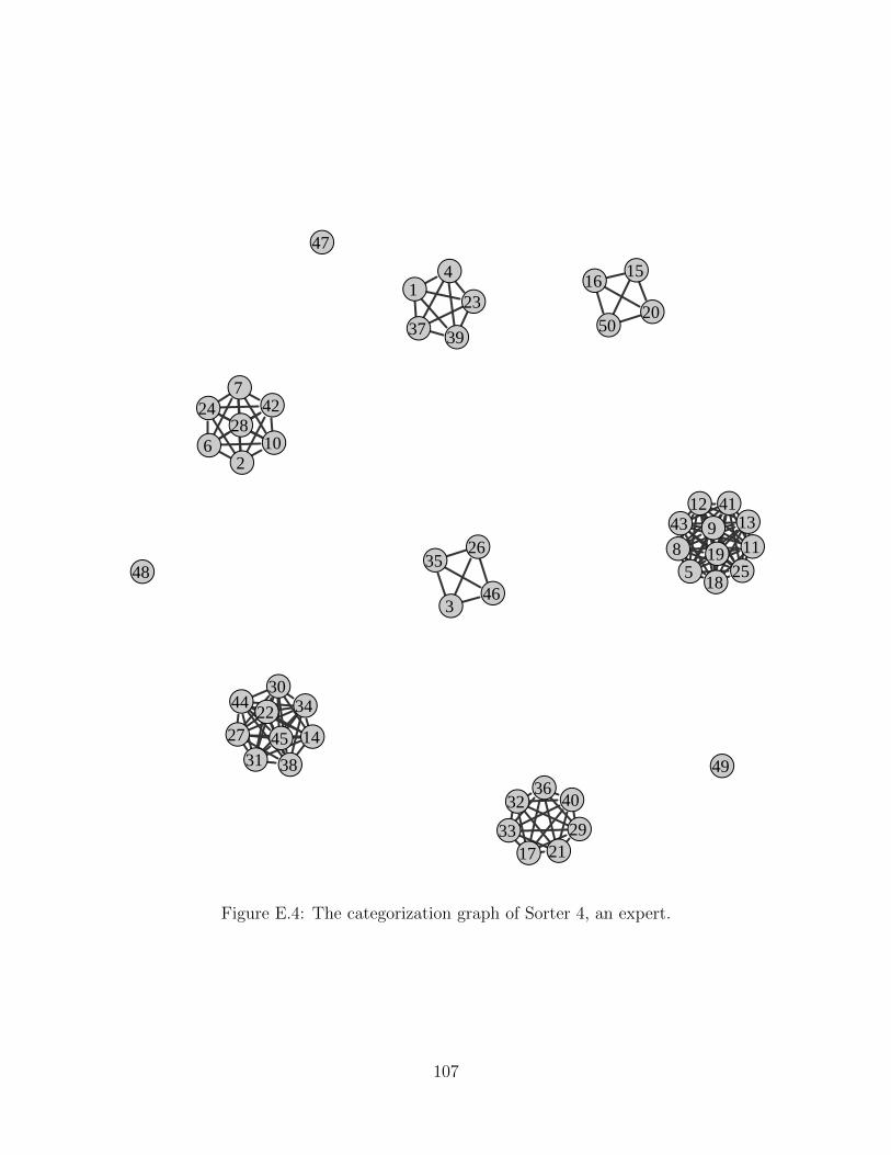
●
●
●
●
●
●
●
●●
●
●
●●
●
●●
●
●●
●
●
●
●
●
●●
●
●
●
●
●
●●
●
●
●
●
●
●
●
●
●
●
●
●
●
●
●
●
●
1
2
3
4
5
6
7
89
10
11
1213
14
1516
17
18
19
20
21
22
23
24
2526
27
28
29
30
31
32
33
34
35
36
37
38
39
40
41
42
43
44
45
46
47
48
49
50
Figure E.4: The categorization graph of Sorter 4, an expert.
107
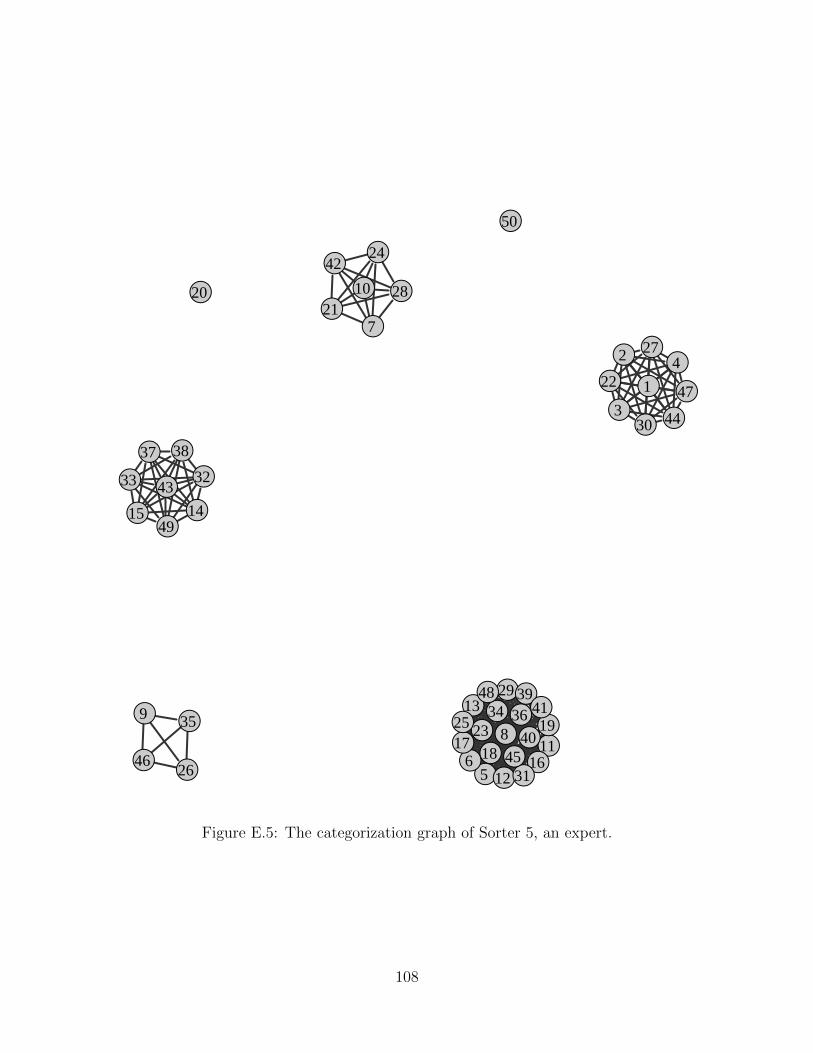
●●
●
●
●●
●
●●
●
●●
●
●●
●● ●
●
●●
●
●
●
●
●
●
●
●
●
●
●●
●● ●
● ●
●
●●
●
●
●
●●
●
●
●
●
1
2
3
4
56
7
89
10
11
12
13
1415
1617
18
19
2021
22
23
24
25
26
27
28
29
30
31
3233
3435 36
37 38
39
40
41
42
43
44
4546
47
48
49
50
Figure E.5: The categorization graph of Sorter 5, an expert.
108
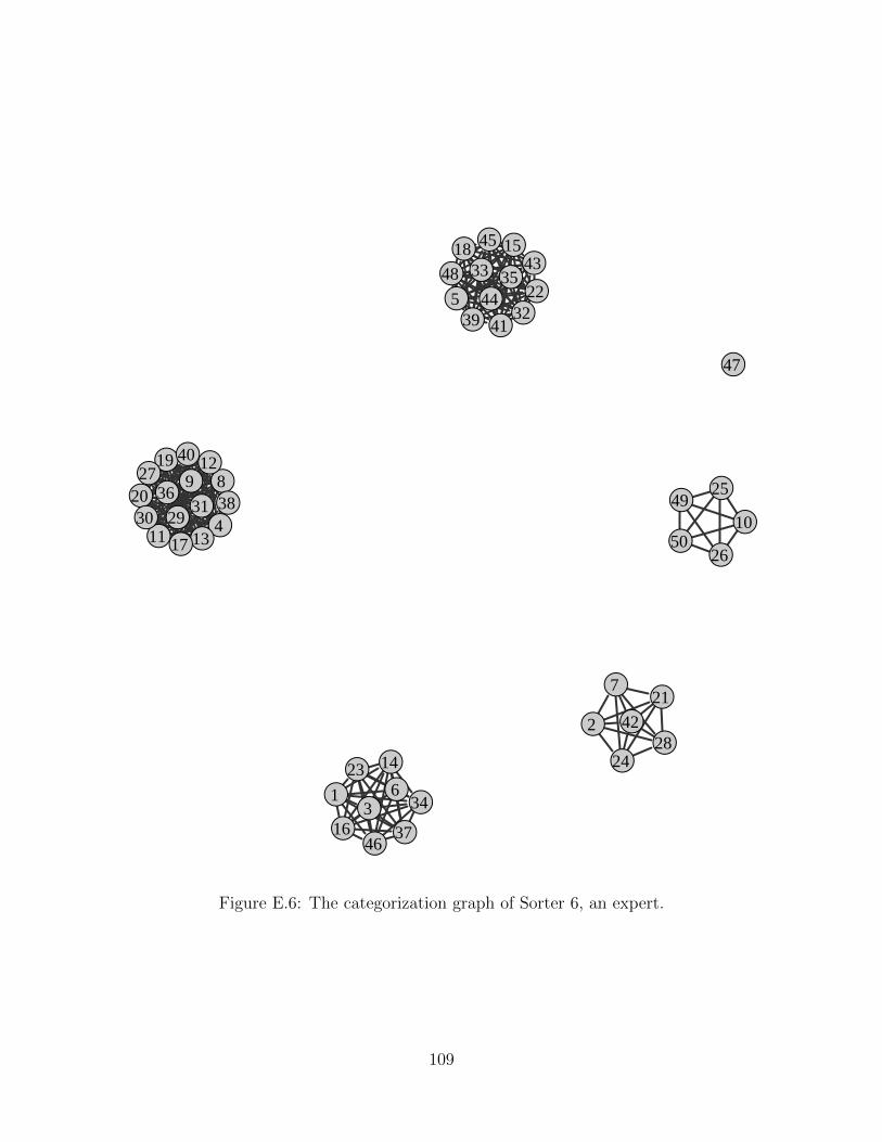
●
●
●
●
●
●
●
●●
●●
●
●
●
●
●
●
●
●
●
●
●
● ●
●
●
●
●
●● ●
●
●
●
●
●
●
●
●
●
●
●
●
●
●
●
●
●
●
●
1
2
3
4
5
6
7
89
1011
12
13
14
15
16
17
18
19
20
21
22
23 24
25
26
27
28
293031
32
33
34
35
36
37
38
39
40
41
42
43
44
45
46
47
48
49
50
Figure E.6: The categorization graph of Sorter 6, an expert.
109
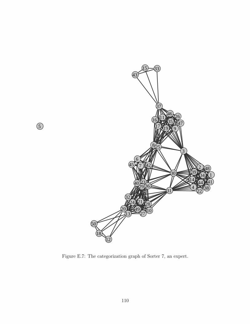
●●
●
●
●
●●
●
●
●
●
●
●
●
●
●●
●
●
●●
●●
●
●
●
●●
●
●
●●
●
●
●
●
●
●
●
● ●
●
●
●
●
●●
●
●
●
1
2
3
4
5
67
8
9
10
11
12
13
14
15
1617
18
19
20
21
22
23
24
25
26
27
28
29
30
3132
33
34
35
36
37
38
39
40 41
42
43
44
45
46
47
48
49
50
Figure E.7: The categorization graph of Sorter 7, an expert.
110
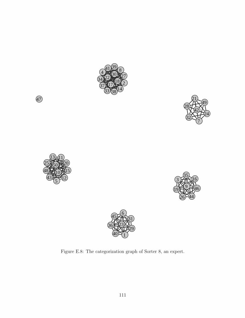
●
●
●
●
●
●
●
●
●
●
●
●
●
●
●●
●●
●
●
●
●
●
●
●
●
●
●
●
●
●
●
●
●
●
●
●●
●
●
●
●
●
●
●
●
●
●
●
●
1
2
3
4
5
6
7
8
9
10
11
12
13
14
15
16
1718
19
20
21
22
23
24
25
26
27
28
29
30
31
32
33
34
35
36
3738
39
40
41
42
43
44
45
46
47
48
49
50
Figure E.8: The categorization graph of Sorter 8, an expert.
111
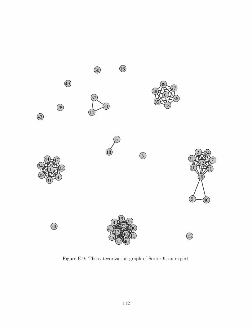
●
●●
●
●
●
●
●
●
●
●●
●●
●
●
●
●
●●
●●
●
●
●
●
●
●
●
●
●
●
●
●
● ●●●
●
●
●
●
●
●
●
●
●
●
●
●
1
23
4
5
6
7
8
9
10
1112
13
14
15
16
17
18
19
20
2122
23
24
25
26
27
28
29
30
31
32
33
34
353637
3839
40
41
42
43
44
45
46
47
48
49
50
Figure E.9: The categorization graph of Sorter 9, an expert.
112
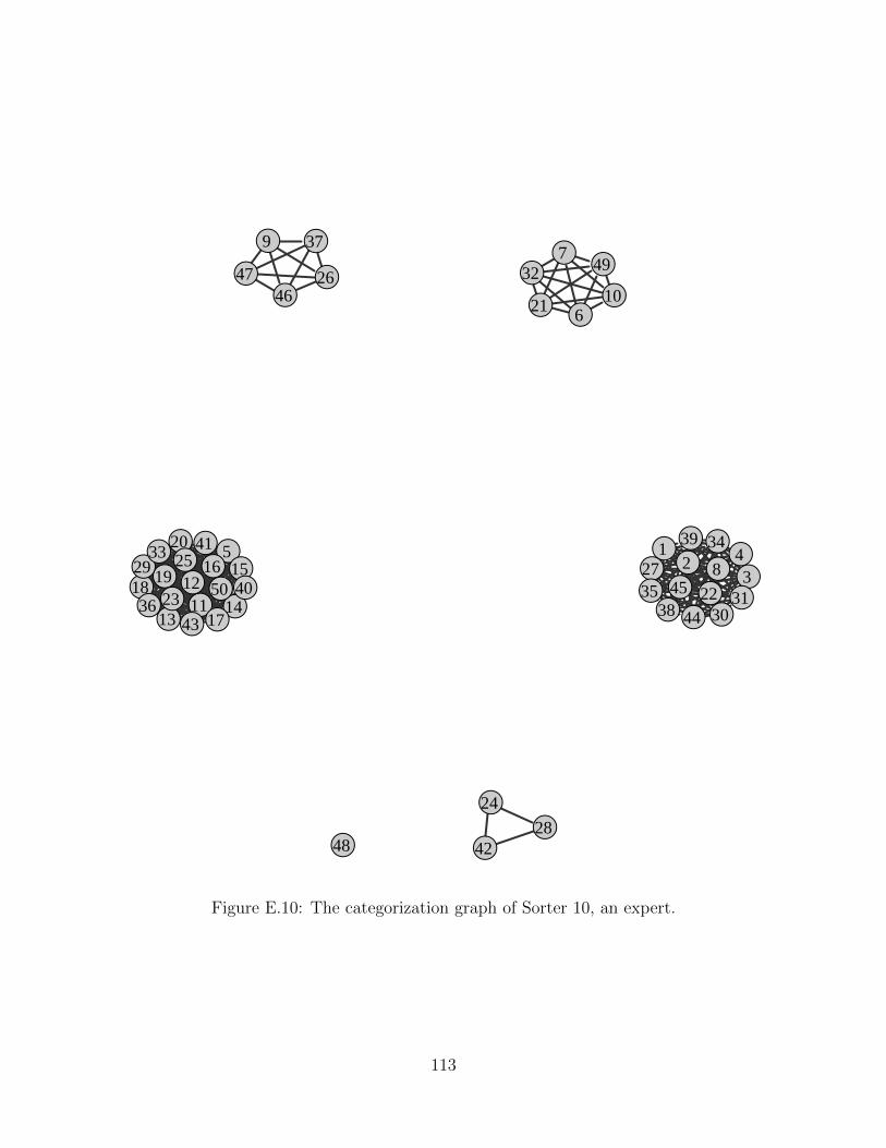
●● ●●●
●
●
●
●
●
●●
● ●
●●
●●●
●
●
●●
●
●
●
●
●
●
●●
●
● ●
●●
●
●
●
●
●
●
● ●●
●●
●
●
●
12
345
6
7
8
9
10
1112
1314
1516
17
1819
20
21
2223
24
25
26
27
28
29
3031
32
3334
3536
37
38
39
40
41
42
43 44
45
4647
48
49
50
Figure E.10: The categorization graph of Sorter 10, an expert.
113

●
●
●
●
●
●
●
●
●
●
●●●
●
●
●
●●
●
●
●●
●
●
●
●
●
●
●
●
●
●
●
●
●
●
●●
●
●
●
●
●
●
●
●
●
●
●
●
1
2
3
4
5
6
7
8
9
10
1112
13
14
15
16
17
18
19
20
21
22
23
24
25
26
27
28
29
30
31
32
33
34
35
36
37
38
39
40
41
42
43
44
45
46
47
48
49
50
Figure E.11: The categorization graph of Sorter 11, an expert.
114
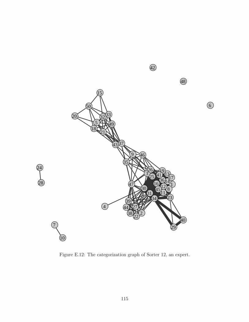
●
●
●
●
●
●
●
●
●
●
●●
●●
●
●●
●
●
●
●
●
●
●●●
●
●
●
●●
●●
●
●
●
●
●
●
●
●
●
●
●
●
●
●
●
●
●
1
2
3
4
5
6
7
8
9
10
1112
13
14
15
1617
18
19
20
21
22
23
24
25
26
27
28
29
3031
3233
34
35
36
37
38
39
40
41
42
43
44
45
46
47
48
49
50
Figure E.12: The categorization graph of Sorter 12, an expert.
115
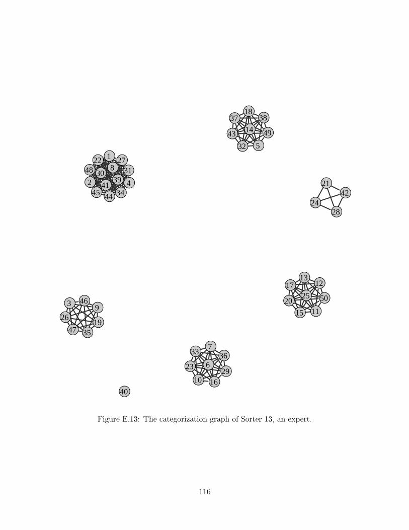
●
●
●
●
●
●
●
●
●
●
●
●●
●
●
●
●
●
●
●
●
●
●
●
●
●
●
●
●
● ●
●
●
●
●
●
● ●
●
●
●●
●
●●
●
●
●
●
●
1
2
3
4
5
6
7
8
9
10
11
1213
14
15
16
17
18
19
20
21
22
23
24
25
26
27
28
29
30 31
32
33
34
35
36
37 38
39
40
4142
43
4445
46
47
48
49
50
Figure E.13: The categorization graph of Sorter 13, an expert.
116
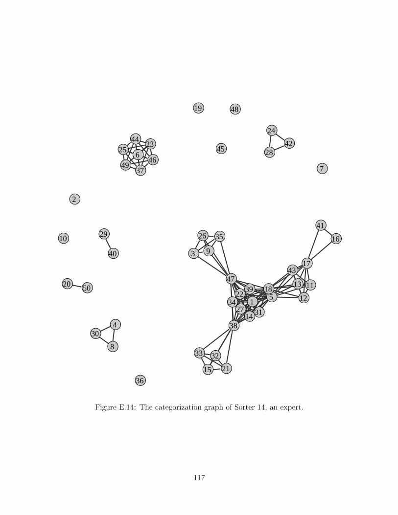
●
●
●
●
●
●●
●
●●
●●
●
●
●
●
●
●
●
●
●
●
●●
●
●
●
●
●
●
●
●●
●
●
●
●
●
●
●
●
●
●
●●
●
●
●
●
●1
2
3
4
5
6
7
8
9
10
11
12
13
14
15
16
17
18
19
20
21
22
23
24
25
26
27
28
29
30
31
3233
34
35
36
37
38
39
40
41
42
43
4445
46
47
48
49
50
Figure E.14: The categorization graph of Sorter 14, an expert.
117
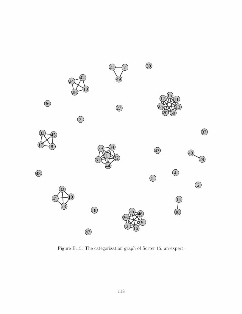
●
●
●
●●
●
●
●
●
●
●●●
●
●
●
●
●
●
●
●
●
●
●
●
●
●
●
●
●
●
●
●
●
●
●
●
●
●●
●
●
●
●
●
●
●
●
●
●
1
2
3
45
6
7
8
9
10
1112
13
14
15
16
17
18
19
20
21
22
23
24
25
26
27
28
29
30
31
32
33
34
35
36
37
38
3940
41
42
43
44
45
46
47
48
49
50
Figure E.15: The categorization graph of Sorter 15, an expert.
118
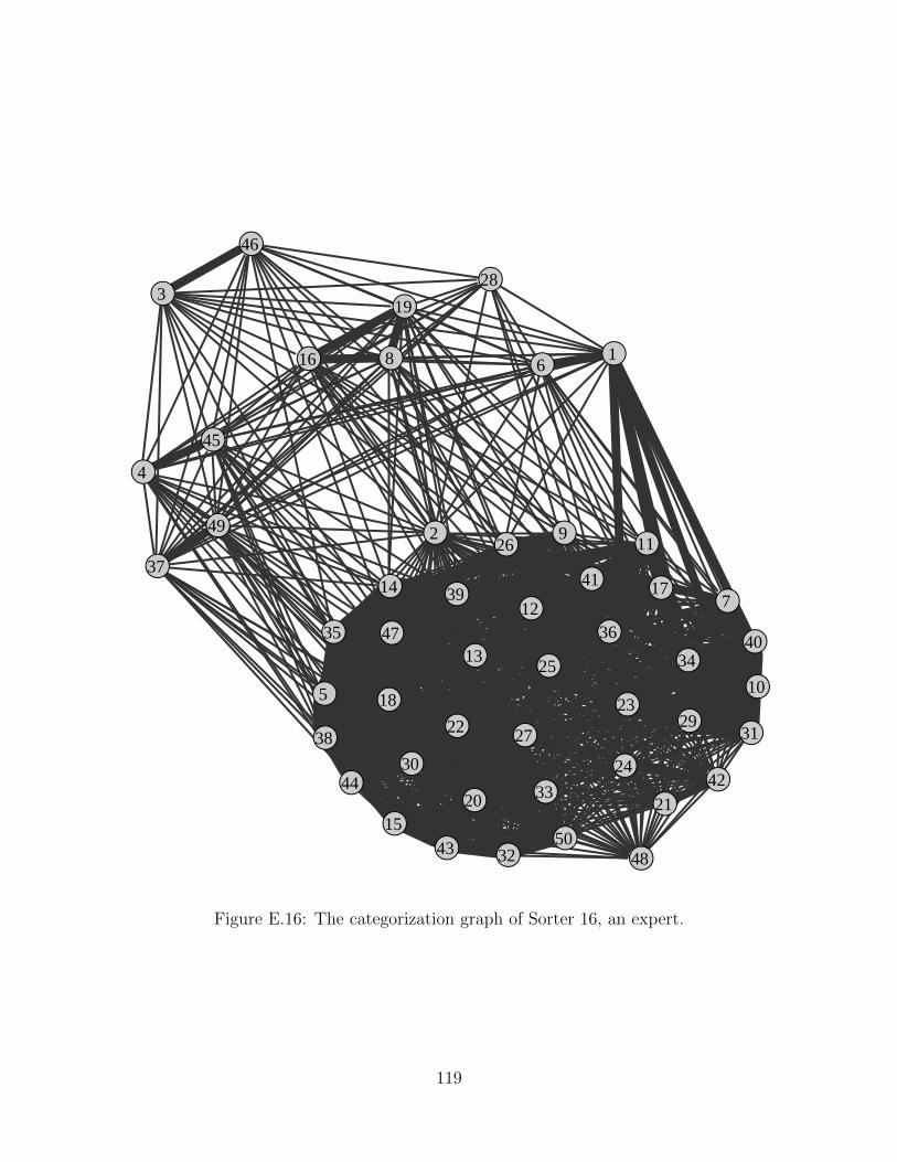
●
●
●
●
●
●
●
●
●
●
●
●
●
●
●
●
●
●
●
● ●
●●
●
●
●
●
●
●
●●
●
●
●● ●
●
●
●
●
●
●
●
●
●
●
●
●
●
●
1
2
3
4
5
6
7
8
9
10
11
12
13
14
15
16
17
18
19
20 21
2223
24
25
26
27
28
29
30
31
32
33
34
35 36
37
38
39
40
41
42
43
44
45
46
47
48
49
50
Figure E.16: The categorization graph of Sorter 16, an expert.
119
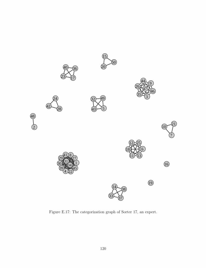
●
●
●
●
●
●
●
●
●
●
●
●
●
●
●
●
●
●
●
●
●
●
●
●
●
●
●
●
●● ●
●
●
●
●
●
●
●
●
●
●
● ●
●
●
●●
●
●
●
1
2
3
4
5
6
7
8
9
10
11
12
13
14
15
16
17
18
19
20
21
22
23
24
25
26
27
28
2930 31
32
33
34
35
36
37
38
39
40
41
4243
44
45
4647
48
49
50
Figure E.17: The categorization graph of Sorter 17, an expert.
120
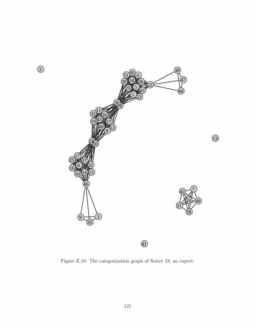
●
●
●
●
●
●
●
●
●
●
●
●
●
●●●
●
●
●
●
●
●
●
●
●
●●
●
●
●
●
●
●
●
●
●
●
●
●●
●
●
●
●●
●
●
●
●
●
1
2
3
4
5
6
7
8
9
10
11
12
13
14 1516
17
18
19
20
21
22
23
24
25
2627
28
29
30
31
32
33
34
35
36
37
38
39
40
41
42
43
4445
46
47
48
49
50
Figure E.18: The categorization graph of Sorter 18, an expert.
121
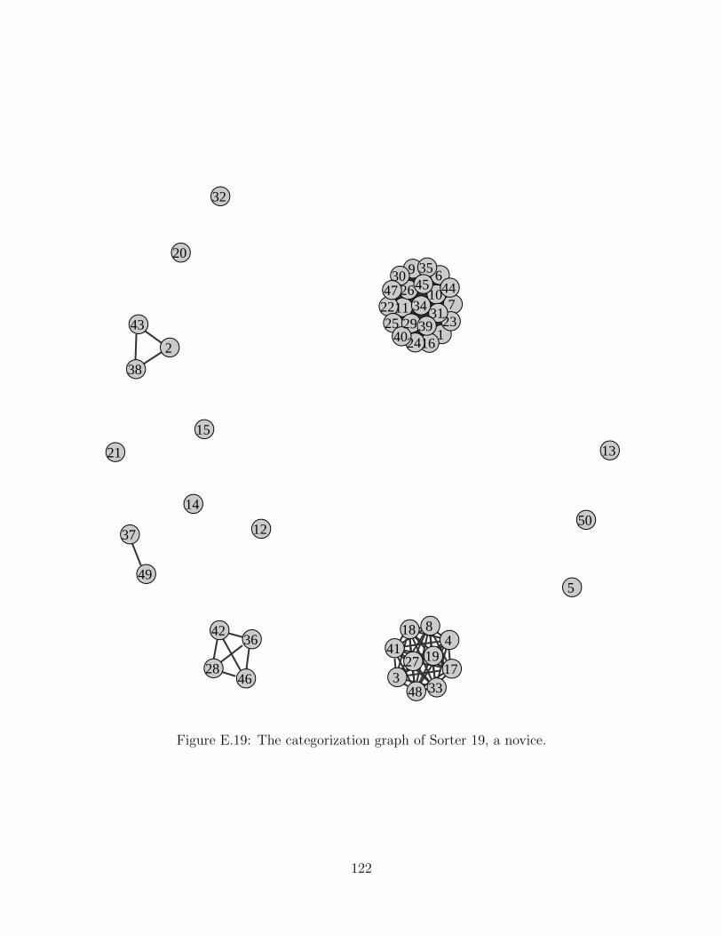
●●
●
●
●
●
●
●
●●
●
●
●
●
●
●
●
●●
●
●
●●
●●
●
●●
●
●
●
●
●
●
●
●
●
●
●●
●●
●
●●
●
●
●
●
●
12
3
4
5
6
7
8
9
1011
12
13
14
15
16
17
18
19
20
21
2223
2425
26
2728
29
30
31
32
33
34
35
36
37
38
3940
4142
43
4445
46
47
48
49
50
Figure E.19: The categorization graph of Sorter 19, a novice.
122
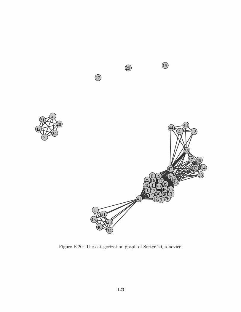
●
●
●
●
●●
●
●●
●●●●
●
●
● ● ●●●
●
●
●
●
●
●
●
●
●
●
●
●●
●
●●
●●
●
●
●
●
●
●
●
●
●
●
●
●
1
2
3
4
56
7
89
1011
12
13
14
15
16 17 1819
20
21
22
23
24
25
26
27
28
29
30
31
32
33
34
3536
37
38
39
40
41
42
43
44
45
46
47
48
49
50
Figure E.20: The categorization graph of Sorter 20, a novice.
123
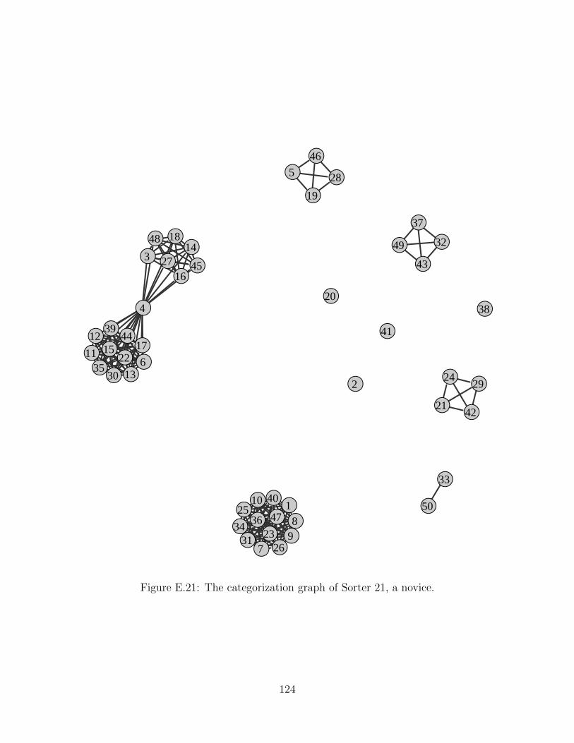
●
●
●
●
●
●
●
●●
●
●●
●
●
●
●
●
●
●
●
●
●
●
●
●
●
●
●
●●
●
●
●
●
●
●
●
●●
●
●
●
●
●
●
●
●
● ●
●1
2
3
4
5
6
7
89
10
11
12
13
14
15
16
17
18
19
20
21
22
23
24
25
26
27
28
2930
31
32
33
34
35
36
37
38
39
40
41
42
43
44
45
46
47
4849
50
Figure E.21: The categorization graph of Sorter 21, a novice.
124
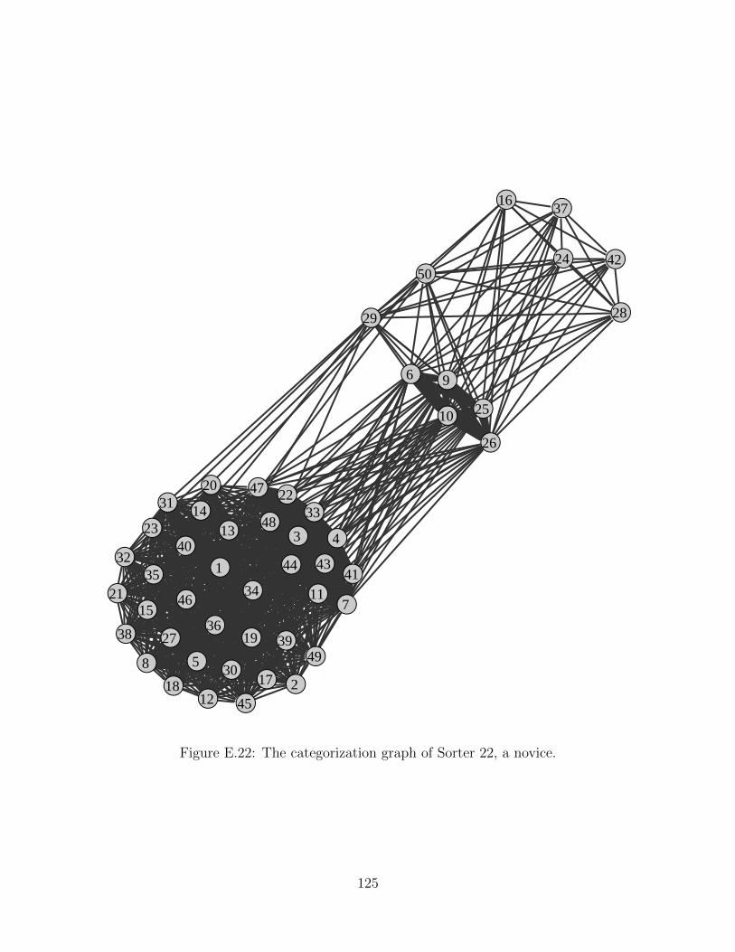
●
●
● ●
●
●
●
●
●
●
●
●
●●
●
●
●●
●
●
●
●
●
●
●
●
●
●●
●
●
●
●
●●
●
●
● ●
●●
●
●●
●
●
●
●
●
●
1
2
3 4
5
6
7
8
9
10
11
12
1314
15
16
1718
19
20
21
22
23
24
25
26
27
2829
30
31
32
33
3435
36
37
38 39
40
41
42
4344
45
46
47
48
49
50
Figure E.22: The categorization graph of Sorter 22, a novice.
125
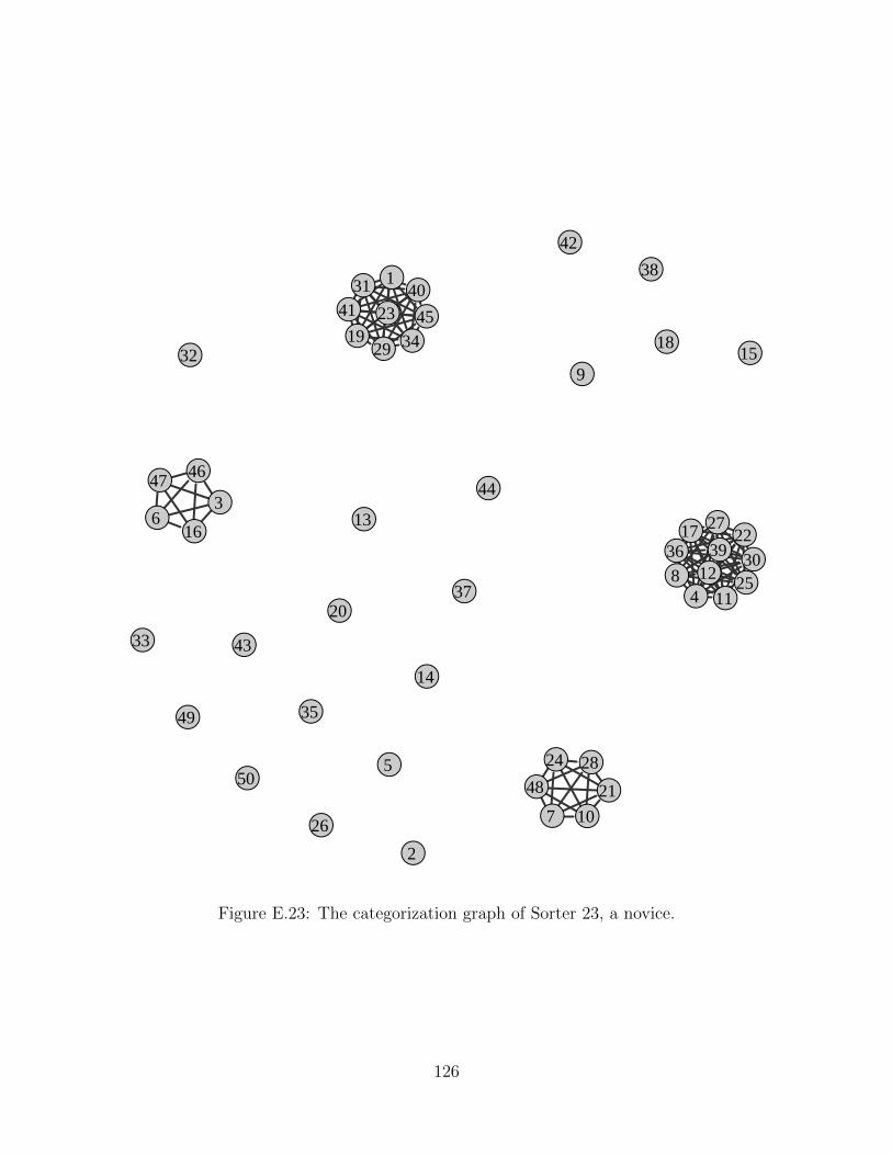
●
●
●
●
●
●
●
●
●
●
●●
●
●
●
● ●
●●
●
●
●
●
●
●
●
●
●
●
●
●
●
●
●
●
●
●
●
●
●●
●
●
●
●
●●
●
●
●
1
2
3
4
5
6
7
8
9
10
11
12
13
14
15
16 17
1819
20
21
22
23
24
25
26
27
28
29
30
31
32
33
34
35
36
37
38
39
4041
42
43
44
45
4647
48
49
50
Figure E.23: The categorization graph of Sorter 23, a novice.
126
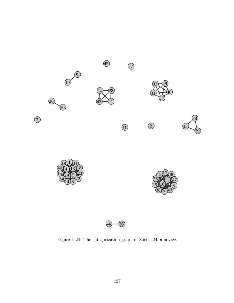
●
●
●
●●●
●
●
●●
●●
●
●●
●
●●
●
● ●
●●
●
●
●
●
●
●
●
●
●●
●
●
●
●
●
●
●
●
●
●
●
●
●
●●
●
●
1
2
3
45
6
7
8
9
10
1112
13
14
15
16
1718
19
20 21
2223
24
25
26
27
28
29
30
31
32
33
34
35
36
37
38
39
40
41
42
43
44
45
46
4748
49
50
Figure E.24: The categorization graph of Sorter 24, a novice.
127
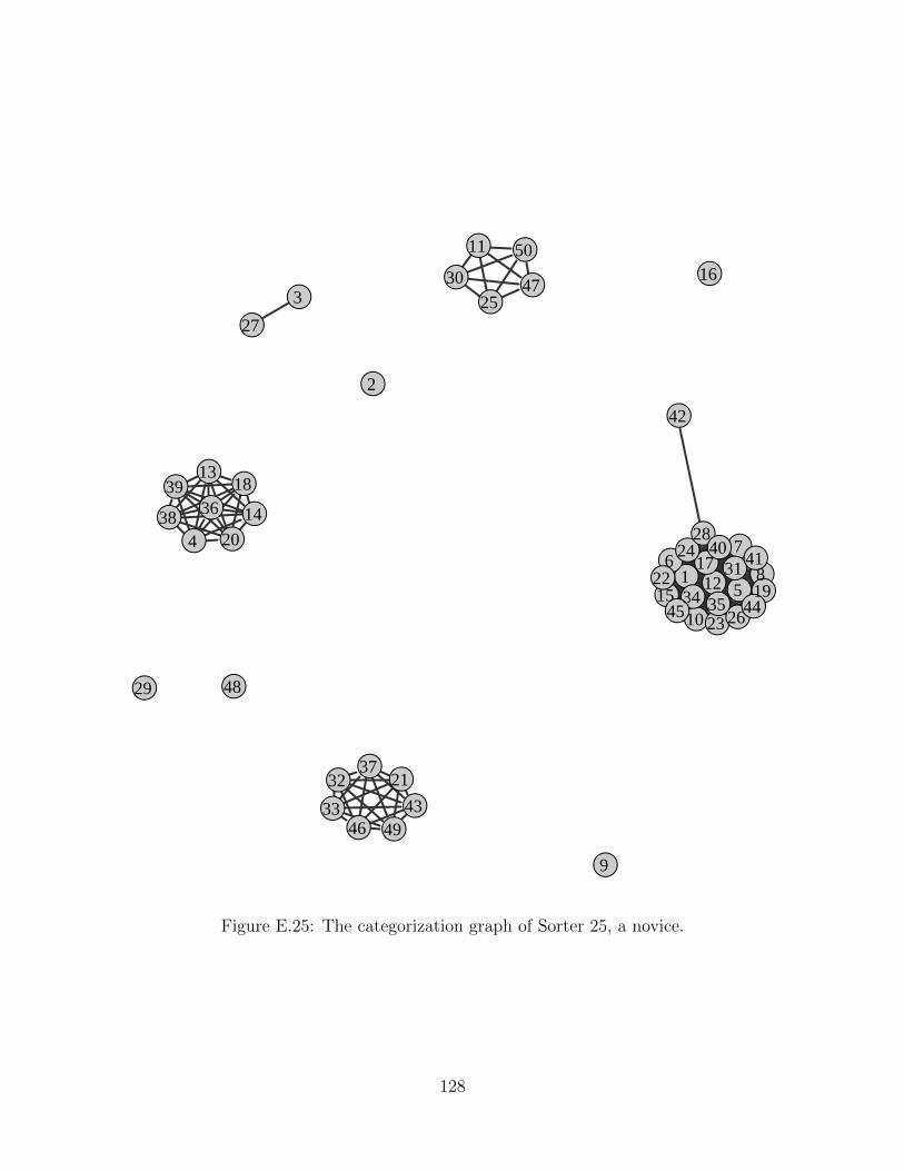
●
●
●
●
●● ●
●
●
●
●
●
●
●
●
●
●
●
●
●
●
●
●
●
●
●
●
●
●
●
●
●●
●●
●
●
●●
● ●
●
●
●●
●
●
●
●
●
1
2
3
4
5
67
8
9
10
11
12
13
14
15
16
17
18
19
20
21
22
23
24
25
26
27
28
29
30
31
32
33
34 35
36
37
38
39
4041
42
43
4445
46
47
48
49
50
Figure E.25: The categorization graph of Sorter 25, a novice.
128
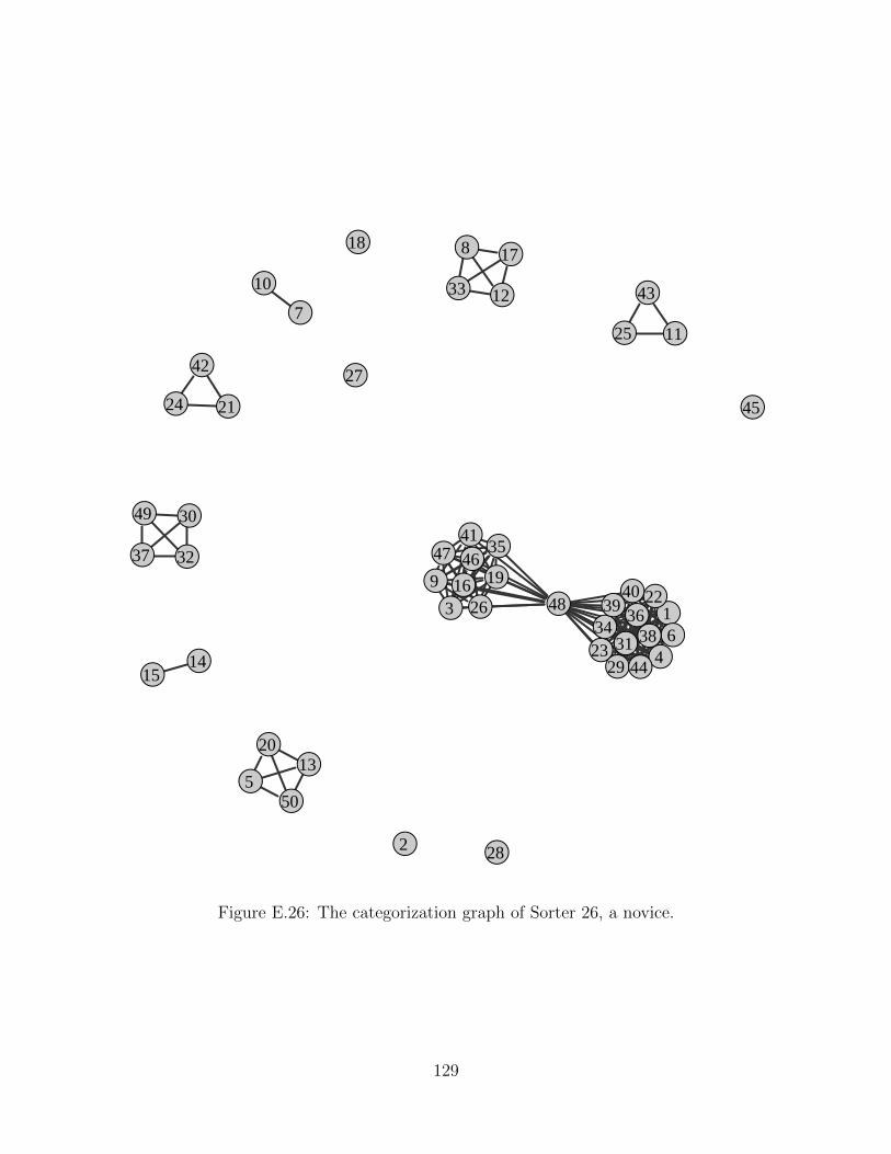
●
●
●
●
●
●
●
●
●
●
●
●
●
●●
●
●●
●
●
●
●
●
●
●
●
●
●
●
●
●
●
●
●
●
●
●
●●●
●
●
●
●
●
●●
●
●
●
1
2
3
4
5
6
7
8
9
10
11
12
13
1415
16
1718
19
20
21
22
23
24
25
26
27
28
29
30
31
32
33
34
35
36
37
38
3940
41
42
43
44
45
4647
48
49
50
Figure E.26: The categorization graph of Sorter 26, a novice.
129

● ●
●
●
●
●●
●
●
●
●
●
● ●
●
●●
●●
●
●●
●
●
●
●
●
●
●
●
●
●●
●
●
●
●
●
●
●
●
●
●
●●
●
●
● ●
●
1 2
3
4
5
6
7
8
9
10
11
12
13 14
15
1617
1819
20
21
22
23
24
25
26
27
28
29
30
31
3233
34
35
36
37
38
39
40
41
42
43
4445
46
47
48 49
50
Figure E.27: The categorization graph of Sorter 27, a novice.
130
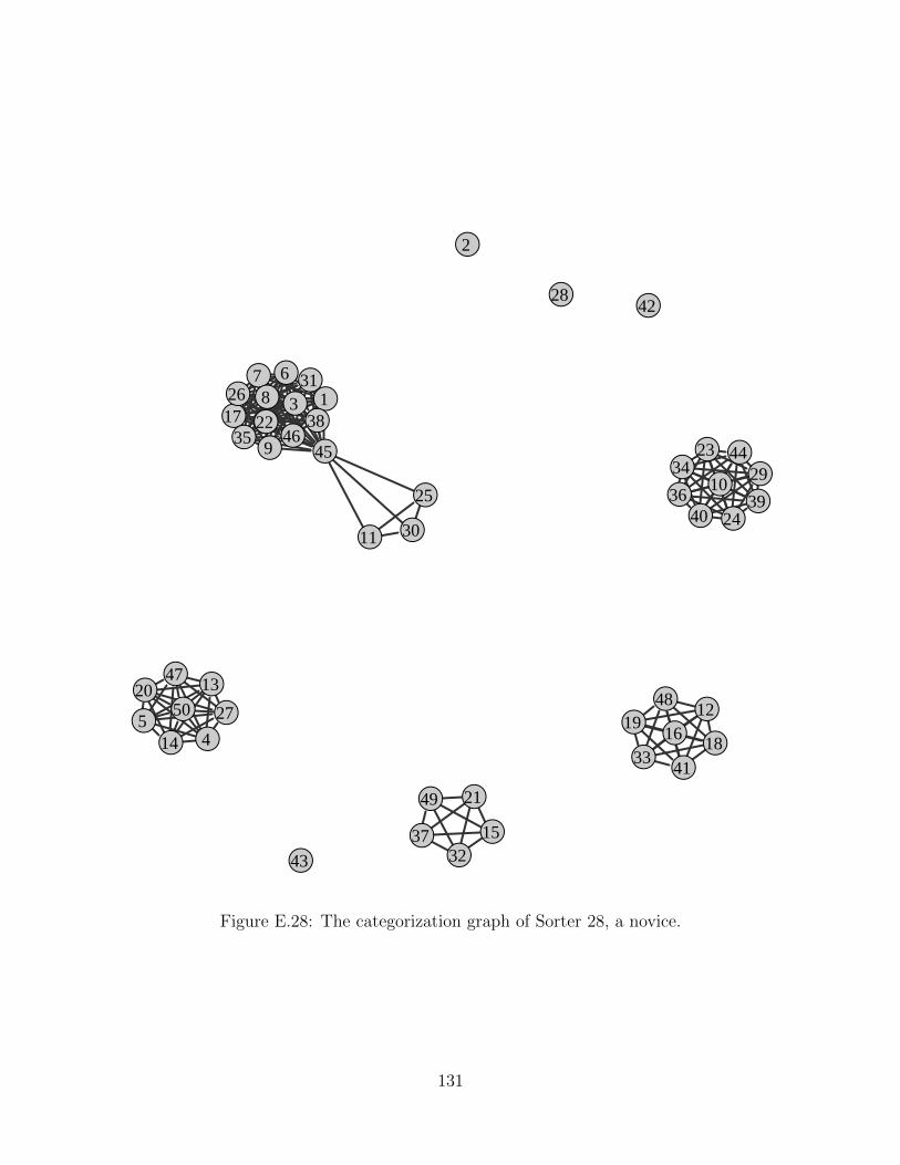
●
●
●
●●
●●●
●
●
●
●●
●
●
●
●
●●
●
●
●●
●●
●
●
●
●
●
●
●
●
●●
●
●
●
●●
●
●
●
●●●
●●
●
●
1
2
3
45
678
9
10
11
12
13
14
15
16
17
1819
20
21
22
23
2425
26
27
28
29
30
31
32
33
34
35
36
37
38
3940
41
42
43
444546
47
48
49
50
Figure E.28: The categorization graph of Sorter 28, a novice.
131
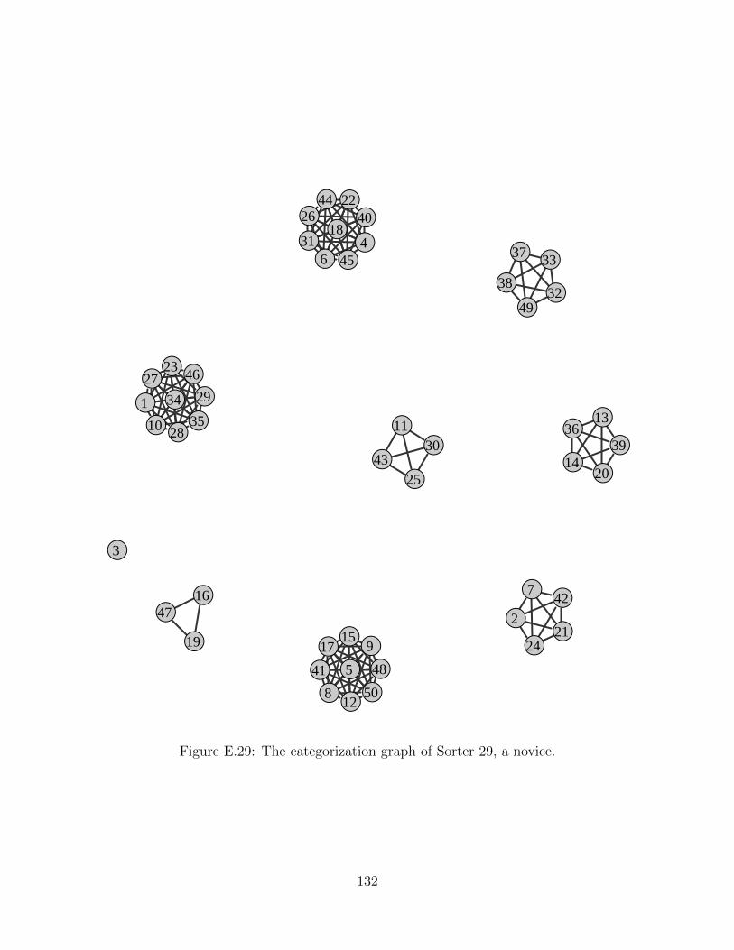
●
●
●
●
●
●
●
●
●
● ●
●
●
●
●
●
●
●
●
●
●
●
●
●
●
●
●
●
●
●
●
●
●
●● ●
●
●
●
●
●
●
●
●
●
●
●
●
●
●
1
2
3
4
5
6
7
8
9
10 11
12
13
14
15
16
17
18
19
20
21
22
23
24
25
26
27
28
29
30
31
32
33
34
35 36
37
38
39
40
41
42
43
44
45
46
47
48
49
50
Figure E.29: The categorization graph of Sorter 29, a novice.
132
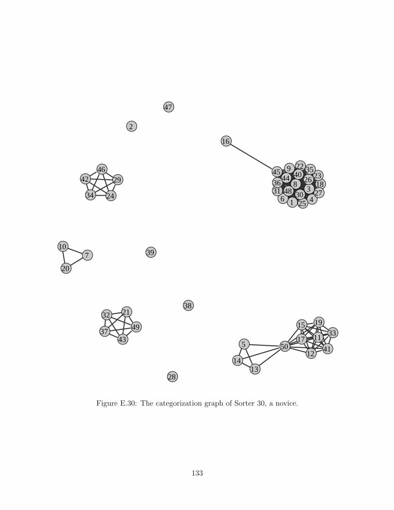
●
●
●●
●
●
●
●●
●
●
●●
●
●
●
●
●
●
●
●
●●
●●
●●
●
●●●
●
●
●
●●
●
●
●
●
●
●
●
●●●
●
●
●
●
1
2
34
5
6
7
8
9
10
11
12
1314
15
16
17
18
19
20
21
2223
2425
26
27
28
29
3031
32
33
34
35
36
37
38
39
40
41
42
43
444546
47
48
49
50
Figure E.30: The categorization graph of Sorter 30, a novice.
133
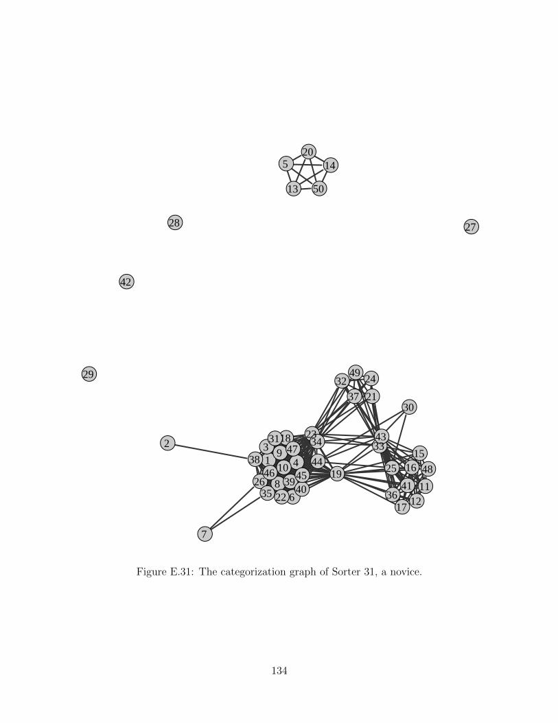
●● ●
●
●
●
●
●
●●
●●
●
●
●●
●
●
●
●
●
●
●
●
●●
●●
●
●
●
●
●●
● ●
●
●●● ●
●
●
●●●
●●
●
●
1
2 3
4
5
6
7
8
910
1112
13
14
1516
17
18
19
20
21
22
23
24
2526
2728
29
30
31
32
3334
35 36
37
38
3940 41
42
43
444546
47
48
49
50
Figure E.31: The categorization graph of Sorter 31, a novice.
134
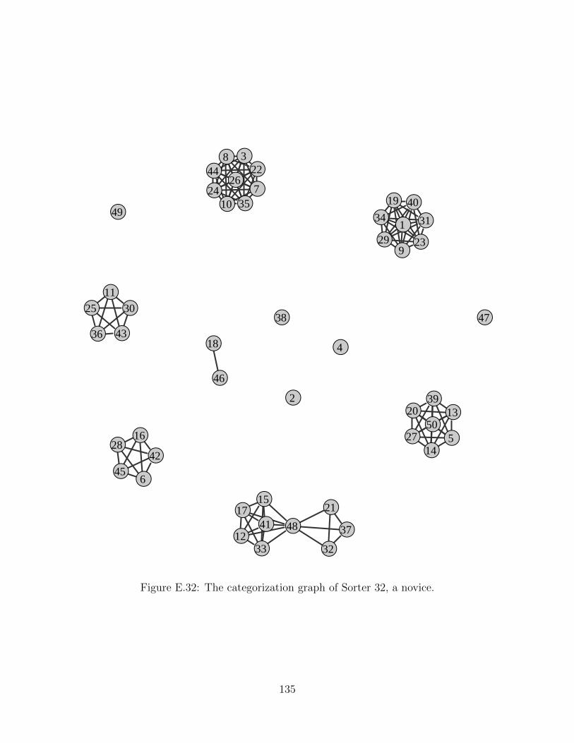
●
●
●
●
●
●
●
●
●
●
●
●
●
●
●
●
●
●
●
●
●
●
●
●
●
●
●●
●
●
●
●●
●●
●
●
●
●
●
●
●
●
●
●
●
●
●
●
●
1
2
3
4
5
6
7
8
9
10
11
12
13
14
15
16
17
18
19
20
21
22
23
24
25
26
2728
29
30
31
3233
3435
36
37
38
39
40
41
42
43
44
45
46
47
48
49
50
Figure E.32: The categorization graph of Sorter 32, a novice.
135
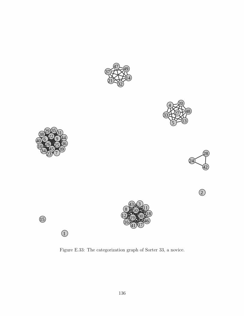
●
●
●
●
●
●
●
●
●●
●●
●
●
● ● ●
●●
●
●
●
●●
●●
●
●
●
●
●
●
●
●
●
●
●
●
●●
●
●
●
●
●
●
●
●
●
●
1
2
3
4
5
6
7
8
9
10
11
12
13
14
1516 17
1819
20
21
22
23
24
2526
27
28
29
30
31
32
33
34
35
36
37
38
39
40
41
42
43
44
45
46
47
48
49
50
Figure E.33: The categorization graph of Sorter 33, a novice.
136

●
●
●
●
●
●
●
●● ●●●
●
●
●
●
● ●●
●
●
●●
●
●
●
●
●●
●
●
●
●●●
●
●
●
●
●
●
●
●
●
●
●
●
●
●●
1
2
3
4
5
6
7
8 9 101112
13
14
15
16
17 1819
20
21
22
23
24
25
26
27
2829
30
31
32
333435
36
37
38
39
40
41
42
43
44
45
46
47
48
4950
Figure E.34: The categorization graph of Sorter 34, a novice.
137
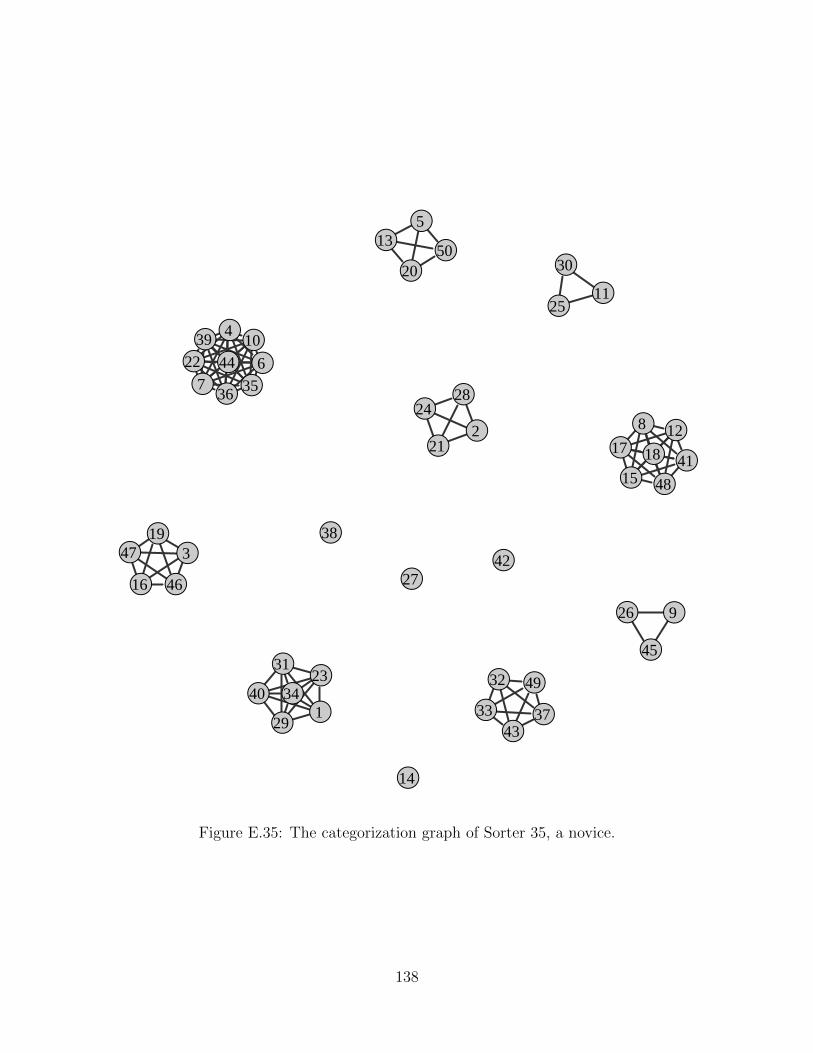
●
●
●
●
●
●●
●
●
●
●
●
●
●
●
●
● ●
●
●
●
●
●
●
●
●
●
●
●
●
●●
●●
●●
●
●
●
●
●
●
●
●
●
●●
●
●
●
1
2
3
4
5
67
8
9
10
11
12
13
14
15
16
17 18
19
20
21
22
23
24
25
26
27
28
29
30
3132
3334
3536
37
38
39
40
41
42
43
44
45
46
47
48
49
50
Figure E.35: The categorization graph of Sorter 35, a novice.
138
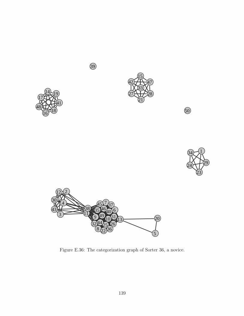
●
●
●
●
●
●●
●
● ●●
●
●
●
●
●
●
●
●
●
●
●
●●
●●
● ●
●
●
●●
●
●
●
●
●●
●
●
●
●
●
●
●●
●
●
●
●
1
2
3
4
5
6
7
8
9 1011
12
13
14
15
16
17
18
19
20
21
22
23
24
25 26
27 28
29
30
31
32
33
34
35
36
3738
39
40
41
42
43
44
4546
47
48
49
50
Figure E.36: The categorization graph of Sorter 36, a novice.
139
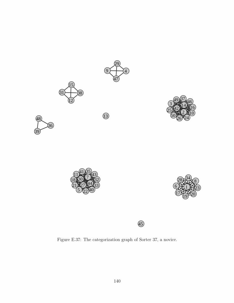
●
●●
●
●●
●●
●
●
●
●
●
●
●
●
●
●
● ●●
● ●
●●
●
●●
●
●
●
●●
●●
●
●●
●
●
●
●
●●
●
●
●
●
●
●
1
2
3
4
56
78
9
10
11
12
13
14
15
16
17
18
19 20
2122
23
24
25
26
2728
29
30
31
3233
34
35
36
3738
39
40
41
42
43
44
45
46
47
48
49
50
Figure E.37: The categorization graph of Sorter 37, a novice.
140
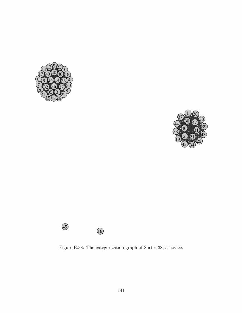
●
●
●
●
●
●●
●
●
●●
●
●
●
●
●
● ●
●
●
●
●
●
● ●
●
●
●
●
●●
●
●
●
●●
●
●●
●
●
●
●
●
●
●●
●●
●
1
2
3
4
5
67
8
9
1011
12
13
14
15
16
17 18
19
20
21
22
23
24 25
26
27
28
29
30
31
32
33
34
3536
37
3839
40
41
42
43
44
45
4647
4849
50
Figure E.38: The categorization graph of Sorter 38, a novice.
141
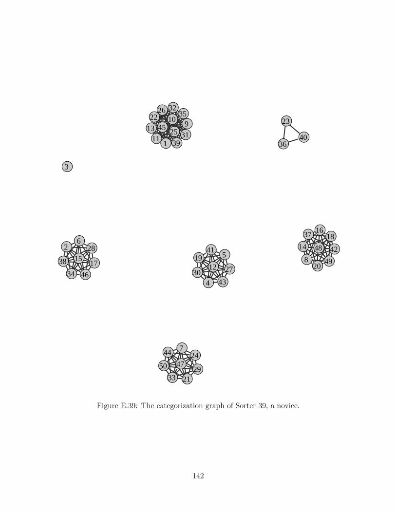
●
●
●
●
●●
●
●
●●
●
●
●
●●
●
●
●
●●
●
● ●
●
●
●
●
●
●
●
●
●
●
●
●
●
●
●
● ●
● ●
●
●
●
●
●
●●
●
1
2
3
4
5
6
7
8
910
11
12
13
14
15
16
17
18
1920
21
22 23
24
25
26
27
28
29
30
31
32
33
34
35
36
37
38
3940
41 42
43
44
45
46
47
48
49
50
Figure E.39: The categorization graph of Sorter 39, a novice.
142

●
●
●
● ●
●
●
●
●
●●
●
●
●●
●
●
●
●
●
●
●
●
●
●
●
●
●
●
● ●●●
●
●
●
●
●
●●
●
●
●
●●
●●
●
●
●
1
2
3
4 5
6
7
8
9
10
11
12
13
1415
16
17
18
19
20
21
22
23
24
25
26
27
28
29
30 313233
34
35
36
37
38
3940
41
42
43
44
45
4647
48
49
50
Figure E.40: The categorization graph of Sorter 40, a novice.
143
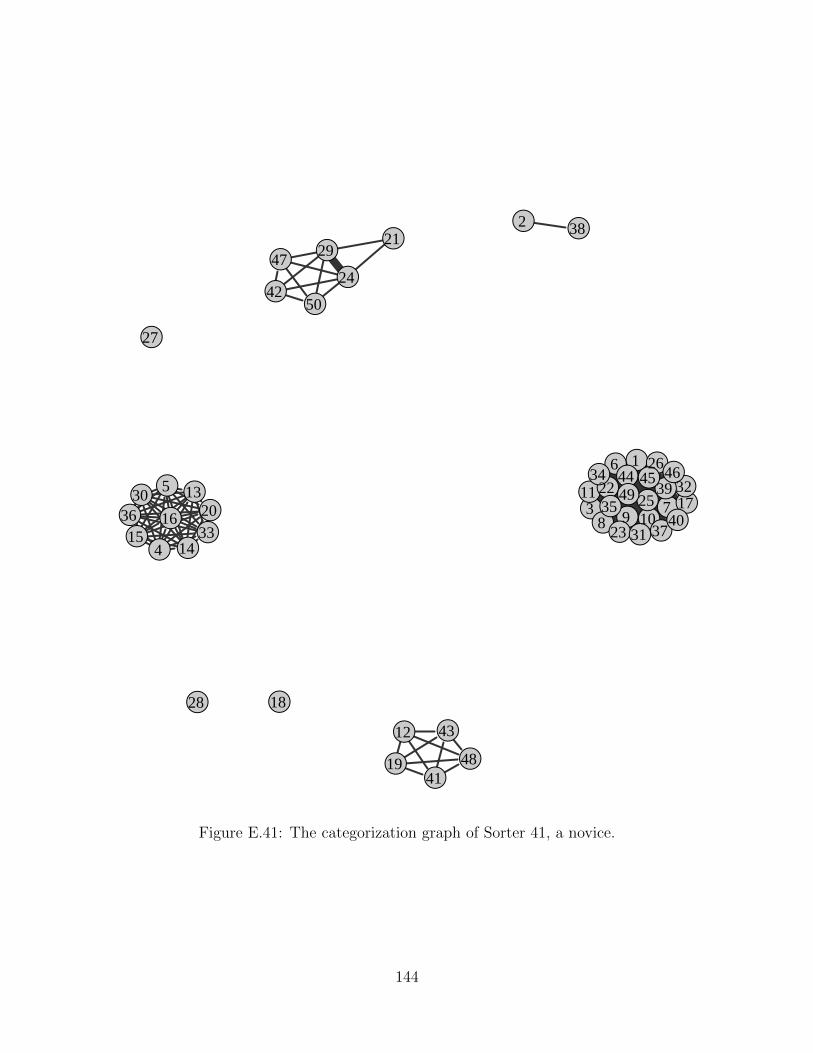
●
●
●
●
●●
●●●●
●
●
●
●●●
●
●
●
●
●
●
●
●
●
●
●
●
●
●
●
●
●
●●●
●
●
●●
●
●
●
●●●
●
●
●
●
1
2
3
4
56
78 9 10
11
12
13
1415
1617
18
19
20
21
22
23
24
25
26
27
28
29
30
31
32
33
34
353637
38
39
40
41
42
43
44 45 46
47
48
49
50
Figure E.41: The categorization graph of Sorter 41, a novice.
144

BIBLIOGRAPHY
145

Bibliography
[1] M. T. H. Chi, P. J. Feltovich, and R. Glaser, Cognitive Science 5, 121 (1981), ISSN0364-0213.
[2] G. H. Veldhuis, Science Education 74, 105 (1990).
[3] G. H. Veldhuis, Ph.D. thesis, Iowa State University (1986), unpublished thesis.
[4] J. S. Walker, Physics (Pearson Education, Inc., Upper Saddle River, New Jersey 07458,2004), 2nd ed., ISBN 0-13-101416-1.
[5] R. Teodorescu, C. Bennhold, and G. Feldman, in Physics Education Research Confer-ence 2008 (Edmonton, Canada, 2008), vol. 1064 of PER Conference, pp. 203–206.
[6] S. F. Wolf, D. P. Dougherty, and G. Kortemeyer, Phys. Rev. ST Phys. Educ. Res. 8,010124 (2012), URL http://link.aps.org/doi/10.1103/PhysRevSTPER.8.010124.
[7] C. Singh, American Journal of Physics 77, 73 (2009).
[8] J. Larkin, J. McDermott, D. P. Simon, and H. A. Simon, Science 208, 1335 (1980).
[9] R. G. Fuller, Physics Today 35, 43 (1982).
[10] G. L. Murphy and J. C. Wright, Journal of Experimental Psychology: Learning, Mem-ory, and Cognition 10, 144 (1984).
[11] K. E. Johnson, P. Scott, and C. B. Mervis, Journal of Experimental Child Psychology87, 171 (2004).
[12] G. E. A. Solomon, The Journal of the Learning Sciences 6, pp. 41 (1997).
[13] M. L. Means and J. F. Voss, Journal of Memory and Language 24, 746 (1985).
[14] D. Hammer, American Journal of Physics 68, S52 (2000), URLhttp://link.aip.org/link/?AJP/68/S52/1.
[15] A. A. diSessa, Cognition and Instruction 10, pp. 105 (1993), ISSN 07370008, URLhttp://www.jstor.org/stable/3233725.
[16] R. E. Scherr, American Journal of Physics 75, 272 (2007), URLhttp://link.aip.org/link/?AJP/75/272/1.
146

[17] B. W. Frank, S. E. Kanim, and L. S. Gomez, Phys. Rev. ST Phys. Educ. Res. 4, 020102(2008), URL http://link.aps.org/doi/10.1103/PhysRevSTPER.4.020102.
[18] T. de Jong and M. G. Ferguson-Hessler, Journal of Educational Psychology 78, 249(1986).
[19] A. Mason and C. Singh, Master’s thesis, University of Pittsburgh, Pittsburgh, PA, USA(2009), unpublished thesis.
[20] A. Mason and C. Singh, Phys. Rev. ST Phys. Educ. Res. 7, 020110 (2011), URLhttp://link.aps.org/doi/10.1103/PhysRevSTPER.7.020110.
[21] S.-Y. Lin and C. Singh, European Journal of Physics 31, 57 (2010).
[22] M. T. H. Chi, personal communication (2010).
[23] G. Milligan, Psychometrika 45, 325 (1980), 10.1007/BF02293907.
[24] R Development Core Team, R: A Language and Environment for Statistical Computing,R Foundation for Statistical Computing, Vienna, Austria (2010), ISBN 3-900051-07-0,URL http://www.R-project.org.
[25] G. Csardi and T. Nepusz, InterJournal Complex Systems, 1695 (2006), URLhttp://igraph.sf.net.
[26] T. Kamada and S. Kawai, Information Processing Letters 31, 7 (1989), ISSN 0020-0190,URL http://www.sciencedirect.com/science/article/pii/0020019089901026.
[27] T. M. J. Fruchterman and E. M. Reingold, Software: Practice and Experience 21, 1129(1991), ISSN 1097-024X, URL http://dx.doi.org/10.1002/spe.4380211102.
[28] P. Erdos and A. Renyi, Publicationes Mathematicae 6, 290 (1959).
[29] A.-L. Barabasi and R. Albert, Science 286, 509 (1999).
[30] W. M. Rand, Journal of the American Statistical Association 66, pp. 846 (1971), URLhttp://www.jstor.org/stable/2284239.
[31] L. Hubert and P. Arabie, Journal of Classification 2, 193 (1985), ISSN 0176-4268.
[32] N. X. Vinh, J. Epps, and J. Bailey, in Proceedings of the 26th International Conferenceon Machine Learning, edited by L. Bottou and M. Littman (Omnipress, Montreal,2009), pp. 1073–1080.
[33] H. Hotelling, The Annals of Mathematical Statistics 2, pp. 360 (1931), ISSN 00034851,URL http://www.jstor.org/stable/2957535.
[34] L. Baringhaus and C. Franz, Journal of Multivari-ate Analysis 88, 190 (2004), ISSN 0047-259X, URLhttp://www.sciencedirect.com/science/article/pii/S0047259X03000794.
147
[35] B. A. Wiggins, Applied and Environmental Microbiology 62, 3997 (1996), URLhttp://aem.asm.org/content/62/11/3997.abstract.
[36] H. Hotelling, Biometrika 28, 321 (1936).
[37] S. Kirkpatrick, C. D. Gelatt, and M. P. Vecchi, Science 220, 671(1983), http://www.sciencemag.org/content/220/4598/671.full.pdf, URLhttp://www.sciencemag.org/content/220/4598/671.abstract.
[38] C. J. P. Belisle, Journal of Applied Probability 29, pp. 885 (1992), ISSN 00219002, URLhttp://www.jstor.org/stable/3214721.
148