Embed Size (px)
Citation preview

Mathematisches Forschungsinstitut Oberwolfach
Report No. 32/2005
Explicit Methods in Number Theory
Organised byHenri Cohen (Talence)
Hendrik W. Lenstra (Leiden)
Don B. Zagier (Bonn)
July 17th – July 23rd, 2005
Abstract. These notes contain extended abstracts on the topic of explicitmethods in number theory. The range of topics included modular forms, va-rieties over finite fields, rational and integral points on varieties, class groups,and integer factorization.
Mathematics Subject Classification (2000): 11xx, 12xx, 13xx, 14xx.
Introduction by the Organisers
The workshop Explicit Methods in Number Theory was organised by Henri Cohen(Talence), Hendrik W. Lenstra (Leiden), and Don B. Zagier (Bonn) and was heldJuly 17–23, 2005. Three previous workshops on the topic had been held in 1999,2001, and 2003. The goal of this meeting was to present new methods and resultson concrete aspects of number theory. In many cases, this included computationaland experimental work, but the primary emphasis was placed on the implicationsfor number theory rather than on the computational methods employed.
There was a ‘mini-series’ of five 1-hour morning talks given by Bas Edixhoven,Johan Bosman, Robin de Jong, and Jean-Marc Couveignes on the topic of com-puting the coefficients of modular forms. Let
∆ = q∏
n≥1
(1 − qn)24 =∑
n≥1
τ(n)qn
be Ramanujan’s tau function, a newform of weight 12 for SL2(Z). The speakersexhibited a method to compute τ(p) for p prime in time polynomial in log p.
Some of the other main themes included:

1800 Oberwolfach Report 32/2005
• Modular forms, q-expansions, and Arakelov geometry• Rational and integral points on curves and higher-dimensional varieties• Integer factorization• Counting points on varieties over finite fields• Class groups of quadratic and cubic fields and their relationship to geom-
etry, analysis, and arithmetic.
As always in Oberwolfach, the atmosphere was lively and active, providing anideal environment for the exchange of ideas and productive discussions. This meet-ing was well-attended—with over 50 participants from a variety of backgroundsand with broad geographic representation from all continents, including a numberof younger researchers. There were 30 talks of various lengths, and ample timewas allotted for informal collaboration.

Explicit Methods in Number Theory 1801
Workshop: Explicit Methods in Number Theory
Table of Contents
Bas Edixhoven (joint with Jean-Marc Couveignes, Robin de Jong)On the computation of the coefficients of a modular form, I: introduction . 1803
Bjorn PoonenCharacterizing characteristic 0 function fields . . . . . . . . . . . . . . . . . . . . . . . . . 1805
Kiran S. KedlayaComputing zeta functions of surfaces . . . . . . . . . . . . . . . . . . . . . . . . . . . . . . . . 1808
E. Victor Flynn (joint with Nils Bruin)Annihilation of Sha on Jacobians . . . . . . . . . . . . . . . . . . . . . . . . . . . . . . . . . . . 1810
John VoightComputing maximal orders of quaternion algebras . . . . . . . . . . . . . . . . . . . . . 1812
Fernando Rodriguez-VillegasRatios of factorial and algebraic hypergeometric functions . . . . . . . . . . . . . . 1813
Johan Bosman (joint with Bas Edixhoven)On the computation of the coefficients of a modular form, II: explicitcalculations . . . . . . . . . . . . . . . . . . . . . . . . . . . . . . . . . . . . . . . . . . . . . . . . . . . . . . 1816
Thorsten KleinjungPolynomial Selection for NFS I . . . . . . . . . . . . . . . . . . . . . . . . . . . . . . . . . . . . . 1818
Daniel BernsteinPolynomial Selection for NFS II . . . . . . . . . . . . . . . . . . . . . . . . . . . . . . . . . . . . 1819
Frank Calegari (joint with Nathan Dunfield)Automorphic forms and rational homology spheres . . . . . . . . . . . . . . . . . . . . . 1820
Jurgen Kluners (joint with Etienne Fouvry)Cohen–Lenstra heuristics for 4–ranks of class groups of quadratic numberfields . . . . . . . . . . . . . . . . . . . . . . . . . . . . . . . . . . . . . . . . . . . . . . . . . . . . . . . . . . . . 1821
Dongho ByeonClass numbers, elliptic curves, and hyperelliptic curves . . . . . . . . . . . . . . . . . 1823
Michael StollFinite coverings and rational points . . . . . . . . . . . . . . . . . . . . . . . . . . . . . . . . . 1824
Robin de Jong (joint with Jean-Marc Couveignes, Bas Edixhoven)On the computation of the coefficients of a modular form, III: Applicationof Arakelov intersection theory . . . . . . . . . . . . . . . . . . . . . . . . . . . . . . . . . . . . . . 1827
Neeraj KayalSolvability of polynomial equations over finite fields . . . . . . . . . . . . . . . . . . . . 1828
1802 Oberwolfach Report 32/2005
Mark WatkinsRandom matrix theory and Heegner points . . . . . . . . . . . . . . . . . . . . . . . . . . . 1829
Bas Edixhoven (joint with Jean-Marc Couveignes, Robin de Jong)On the computation of the coefficients of a modular form, IV: theArakelov contribution . . . . . . . . . . . . . . . . . . . . . . . . . . . . . . . . . . . . . . . . . . . . . . 1830
Samir Siksek (joint with Martin Bright)Functions, reciprocity and the obstruction to divisors on curves . . . . . . . . . 1832
Michael A. Bennett (joint with P.G. Walsh)Integral points on congruent number curves . . . . . . . . . . . . . . . . . . . . . . . . . . . 1835
Bart de Smit (joint with Lara Thomas)Local Galois module structure for Artin-Schreier extensions of degree p . . 1837
Nicole RaulfHecke operators and class numbers . . . . . . . . . . . . . . . . . . . . . . . . . . . . . . . . . . 1838
Reinier BrokerClass invariants in a non-archimedean setting . . . . . . . . . . . . . . . . . . . . . . . . 1839
Ronald van LuijkExplicit computations on the Manin conjectures . . . . . . . . . . . . . . . . . . . . . . . 1841
Jean-Marc CouveignesOn the computation of the coefficients of a modular form, V: computationalaspects . . . . . . . . . . . . . . . . . . . . . . . . . . . . . . . . . . . . . . . . . . . . . . . . . . . . . . . . . . . 1842
Tim Dokchitser (joint with Vladimir Dokchitser)Computations in non-commutative Iwasawa theory of elliptic curves . . . . . 1846
William A. Stein (joint with G. Grigorov and A. Jorza and S. Patrikis andC. Tarnita-Patrascu)Computational verification of the Birch and Swinnerton-Dyer conjecturefor individual elliptic curves . . . . . . . . . . . . . . . . . . . . . . . . . . . . . . . . . . . . . . . . 1848
H.M. StarkThe Brauer-Siegel theorem . . . . . . . . . . . . . . . . . . . . . . . . . . . . . . . . . . . . . . . . . 1850
Robert CarlsTheta null points of canonical lifts . . . . . . . . . . . . . . . . . . . . . . . . . . . . . . . . . . 1853
Bas JansenMersenne primes and class field theory . . . . . . . . . . . . . . . . . . . . . . . . . . . . . . 1855
Mark van Hoeij (joint with Jurgen Kluners)Generating Subfields . . . . . . . . . . . . . . . . . . . . . . . . . . . . . . . . . . . . . . . . . . . . . . . 1858
Explicit Methods in Number Theory 1803
Abstracts
On the computation of the coefficients of a modular form, I:introduction
Bas Edixhoven
(joint work with Jean-Marc Couveignes, Robin de Jong)
The following text is based on notes taken by Bjorn Poonen. I thank him forletting me use his notes. The responsibility for mistakes in this text is mine.As this text has been edited shortly after the conference, it also reflects somecomments from and discussions with the audience.
Let
∆ = q∏
n≥1
(1 − qn)24 =∑
n≥1
τ(n)qn
with q = e2πiz for z ∈ H (the upper half plane). This ∆ is a newform of weight12 for SL2(Z).
If one has the factorization of n, one can easily compute τ(n) in terms of theτ(p) for primes p dividing n. (If one can compute the coefficient σk−1(n) of theEisenstein series Ek, one can go backwards, and factor n. It’s not clear that onecan do this for τ .)
Theorem 1 (Deligne 1969). For all primes ℓ, there is a unique continuous semisim-ple representation
ρℓ : Gal(Q/Q) → GL(Vℓ)
where Vℓ is a 2-dimensional Fℓ-vector space, unramified outside ℓ, such that forall primes p 6= ℓ,
det(1 − xFrobp |Vℓ) = 1 − xτ(p) + x2p11
in Fℓ[x].
Later Deligne showed also that |τ(p)| < 2p11/2. (Hecke had proved |τ(p)| =O(p6), with an explicit constant, and this will suffice for our purposes.)
Aim of the project:
(1) To show that ρℓ can be computed in time polynomial in ℓ.(2) To show that for big primes p, the value of τ(p) can be computed in time
polynomial in log p. (Question of Rene Schoof)
The first can be used to do the second. We claim that these can be done indeterministic polynomial time, but our presentation will use randomness.
Theorem 2 (Swinnerton-Dyer and Serre 1972). For ℓ /∈ 2, 3, 5, 7, 23, 691, wehave Im ρℓ ⊇ SL(Vℓ); i.e.,
Im(ρℓ) = g ∈ GL(Vℓ) : det g is an 11-th power.In what follows we will suppose that ℓ /∈ 2, 3, 5, 7, 23, 691.

1804 Oberwolfach Report 32/2005
Theorem 3 (Deligne 1969). The dual representation V ∨ℓ is contained in the 11th
etale cohomology group H11(E10Q,et
,Fℓ) of the 11-dimensional variety that is the
10-th fibered power of the universal elliptic curve over the j-line. Also,
V ∨ℓ = H1(j-line
Q,et, Sym10(R1π∗Fℓ)).
Let Xℓ be the modular curve X1(ℓ), and let Jℓ be its Jacobian. Then Vℓ ⊂Jℓ(Q)[ℓ]. We have
Xℓ(C) = Γ1(ℓ)\(H ∪ P1(Q))
where Γ1(ℓ) is the inverse image in SL2(Z) of the subgroup
(1 ∗
1
)of SL2(Z/nZ).
This is related to the fact that ∆ is congruent modulo ℓ to a weight 2 form oflevel ℓ. The genus of Xℓ is about ℓ2/24. Let Tℓ ⊂ End(Jℓ) be the Hecke algebra,generated by the Tn, n ≥ 1, and 〈a〉, for a ∈ F×
ℓ . As a Z-module, it is free of rankgℓ. Then
Vℓ =⋂
1≤i≤(ℓ2−1)/6
ker(Ti − τ(i), Jℓ(Q)[ℓ]
):
this follows from a multiplicity 1 result and a result of Jacob Sturm bounding thenumber of i needed.
Strategy: Choose an effective divisor D = P1 + · · · + Pgℓof degree gℓ on Xℓ,Q
and a map f : Xℓ,Q ։ P1Q. Then:
X1(C)gℓ → Jℓ(C) = Cgℓ/Λℓ
(Q1, . . . , Qgℓ) 7→ [Q1 + · · · +Qgℓ
−D] =
gℓ∑
i=1
∫ Qi
Pi
(ω1, . . . , ωgℓ),
where the ωi are newforms, normalized by a1(ωi) = 1, and Λℓ = H1(Xℓ(C),Z).Since the induced map Symgℓ Xℓ → Jℓ is a birational morphism, with some luck,for all nonzero x ∈ Vℓ, there exists a unique effective D′
x = Qx,1 + · · · + Qx,gℓ
of degree gℓ with [D′x − D] = x, and D′
x is disjoint from the poles of f . Theuniqueness of D′
x satisfying [D′x − D] = x is equivalent to h0(Xℓ,Q,Lx(D)) = 1,
where Lx is the line bundle corresponding to x.Consider the polynomial
Pℓ :=∏
x∈Vℓ−0(T −
∑
i
f(Qx,i)) ∈ Q[T ]
of degree ℓ2 − 1. One could use a variant∏
lines L⊂Vℓ
(T −∑
06=x∈L
∑
i
f(Qx,i)),
which has degree ℓ+ 1.Now Pℓ can be approximated in C[T ], or computed modulo p in Fp[T ] for many
p.
Explicit Methods in Number Theory 1805
Theorem 4. (not completely written up yet) There exists an explicit c (maybec = 16) such that for all ℓ, one can choose D and f so that the logarithmic heightof the coefficients of Pℓ are O(ℓc).
The proof of this theorem is the subject of lectures 3 and 4 of this series.Choice of D: We will do this on Xℓ redefined as X1(5ℓ), and with D over Q(ζℓ)
(this not change anything above significantly).Idea: Specialize to Xℓ,Fℓ
. As x 0, Lx OXℓ,Fℓ. For a place of Q over ℓ, the
kernel of reduction modulo ℓ in Vℓ is a line if ℓ ∤ τ(ℓ), and is Vℓ if ℓ | τ(ℓ).Note: Gal(Q/Q(ζℓ)) acts transitively on Vℓ−0, and fixesD, so h0(Xℓ,Q,Lx(D))
is independent of x. All we need is that h0(Xℓ,Fℓ,O(D)) = 1. Equivalently by
Riemann-Roch and Serre duality, we need h0(Xℓ,Fℓ,Ω(−D)) = 0.
Let X1, X2 be the two components of Xℓ,Fℓ, and let Σ = X1 ∩ X2. Then
X1 → X1(5)Fℓ
x∼→ P1
Fℓ. The curve X1 has an equation yℓ−1 = f(x) where f has
degree ℓ− 1 and simple zeros, and Σ is the set of zeros of y. Then D = D1 +D2
with D1 on X1 and D2 on X2.Recipe for D1: distribute the multiplicities 0, 1, . . . , ℓ− 2 over the ℓ− 1 zeros of
x on X1. For D2: — 0, 0, 1, 2, . . . , ℓ− 3.
Characterizing characteristic 0 function fields
Bjorn Poonen
Consider first-order formulas in the language of rings. We will not give a precisedefinition of first-order formula here, but loosely speaking it is an expression builtup from the symbols +, ·, 0, 1,=, (, ), the logical relations ∧ (“and”), ∨ (“or”), ¬(“not”), the quantifers ∀ (“for all”) and ∃ (“there exists”), and variables x, y, z, . . . .For instance,
(∀y)(∃z)(∃w) (x · z + 1 + 1 = y2) ∨ ¬(z = x+ w)
is a first-order formula. In this example, the variables y, z, w are bound by quan-tifiers, and the variable x is free. A first-order formula in which all variablesare bound by quantifiers is called a first-order sentence. From now on, it will beunderstood that formulas and sentences are first-order formulas and sentences.
If we fix a ring R, then it is understood that the variables represent elements inR. (In contrast, second-order logic allows variables ranging over subsets.) Thenfor each assignment of elements of R to the free variables, we get a truth value.In particular, a sentence has a truth value for each ring R.
It is important, especially when trying to transfer results from one ring toanother, to know whether a ring-theoretic property can be expressed by the truthof a first-order sentence. For example, it is a basic theorem of model theory thata sentence true for one algebraically closed field of characteristic 0 is true forall algebraically closed fields of characteristic 0; it is because of this that many
1806 Oberwolfach Report 32/2005
theorems proved for C using analytic methods are known to hold for arbitraryalgebraically closed fields of characteristic 0.
By compactness, there does not exist a sentence that for each field K is trueif and only if K is of characteristic 0. We prove that, on the other hand, there isa sentence with this property if we consider only finitely generated fields, that is,fields that are finitely generated (as a field) over the prime subfield. Such fieldsare the finite extensions of rational function fields Fp(t1, . . . , tn) or Q(t1, . . . , tn).
Theorem 1. There is a sentence that is true for all finitely generated fields ofcharacteristic 0, and false for all finitely generated fields of characteristic > 0.
The proof makes use of two earlier results. To state these, we need a fewdefinitions.
Definition 2. The Kronecker dimension of a finitely generated field K is
KrdimK :=
trdeg(K/Fp), if charK = p > 0
trdeg(K/Q) + 1, if charK = 0.
A global field is a finitely generated field K with KrdimK = 1; such a field is eithera number field (finite extension of Q) or a global function field (function field of acurve over a finite field).
Definition 3. The Pfister form 〈〈a1, . . . , an〉〉 is the diagonal quadratic form in 2n
variables whose coefficients are∏
i∈S ai as S ranges through subsets of 1, . . . , n.For example, 〈〈a, b〉〉 is the quadratic form
x21 + ax2
2 + bx23 + abx2
4.
Among other things, R. Rumely proved our Theorem 1 for global fields:
Theorem 4 ([Rum80]). There is a sentence that is true for all number fields andfalse for all global function fields.
Rumely’s idea was to build on work of J. Robinson to define the family ofvaluation rings of a global field K in a uniform first-order way, and then to observethat a global field is a number field if and only if the intersection of the valuationrings is not a field.
F. Pop, as part of his work on the “elementary equivalence versus isomorphism”problem for finitely generated fields, discovered that recent work on isotropy ofPfister forms could be used to characterize fields of given Kronecker dimension:
Theorem 5 ([Pop02]). For each n ∈ N and finitely generated field K, we haveKrdimK ≤ n if and only if either
• 2 = 0 and [K : K2] ≤ 2n, or• 2 6= 0 and every Pfister form 〈〈a1, . . . , an+2〉〉 over K(
√−1) represents 0
over K(√−1).
Thus, for each n ∈ N, there is a sentence σn that for a finitely generated field Kholds if and only if KrdimK = n.

Explicit Methods in Number Theory 1807
Definition 6. If φ is a first-order formula with n + 1 free variables, then forany field K, the set of a ∈ Kn+1 satisfying φ is a subset A ⊆ Kn+1. We havea projection Kn+1
։ Kn that discards the last coordinate. The fibers of thecomposition A → Kn+1
։ Kn form a family of subsets of K. Such a family willbe called a definable family of subsets. We will call it a uniformly definable family of
subsets in the situation where we have a definable family of subsets of K for manydifferent fields K, and the formula that defines it is independent of K.
Now we list the main steps in the proof of Theorem 1. It suffices to find asentence that works for the finitely generated fields with
√−1 ∈ K, so we assume
this from now on. In the case where charK = 0, we let k be the relative algebraicclosure of Q in K, so k is a number field. With this notation, the following stepsgive a proof that there is a uniformly definable family F of K such that wheneverK is a finitely generated field of characteristic 0 containing
√−1, we have k ∈ F .
(1) Prove that there exists an elliptic curve E over Q such that E(Q) is infiniteand E(K) = E(k). The key here is to reinterpret E(K) as the set of k-rational maps Alb V 99K Ek where AlbV is the Albanese variety of ak-variety V with function field K, and Ek = E ×Q k.
(2) Observe that for such E, the set of values of the rational function x/y (auniformizing parameter at ∞ for a Weierstrass model) on E(K) is a subsetR of k such that R ∩ Q is p-adically dense in a neighborhood of 0 in Qp
for all primes p.(3) Ratios of elements from this R form a subset S of k such that S ∩ Q is
p-adically dense in Qp for all primes p.(4) For t ∈ K,
t ∈ k ⇐⇒ ∀s1, s2, s3 ∈ S, 〈〈s1, s2, t− s3〉〉 represents 0 over K.
(5) For each (a, b) ∈ K2, we get a curve E : y2 = x3 + ax + b over K, and asubset of K defined in the previous step. These form a uniformly definablefamily F of subsets indexed by (a, b) ∈ K2. If (a, b) define the special Edescribed in the first step, then the corresponding subset of K equals k.
Now, given any finitely generated field K containing√−1, we can say that
charK = 0 if and only if there exists a subset S ∈ F such that S is a field andKrdimS = 1 and S is a number field. The conditions on S can be expressed in afirst-order sentence, because of Theorems 4 and 5. This completes the sketch ofthe proof of Theorem 1.
With a lot more work, one can find also a formula with one free variable thatfor any finitely generated field K defines the relative algebraic closure k of theprime field in K, and a formula φn(x1, . . . , xn) with n free variables that holds ina finitely generated field K for elements x1, . . . , xn if and only if x1, . . . , xn arealgebraically dependent over k.
One can also prove some geometric analogues, for function fields over alge-braically closed or other large fields: these geometric analogues will appear in ajoint paper with F. Pop.

1808 Oberwolfach Report 32/2005
References
[Pop02] Florian Pop, Elementary equivalence versus isomorphism, Invent. Math. 150 (2002),no. 2, 385–408. MR1933588 (2003i:12016).
[Rum80] R.S. Rumely, Undecidability and definability for the theory of global fields,Trans. Amer. Math. Soc. 262 (1980), no. 1, 195–217. MR583852 (81m:03053).
Computing zeta functions of surfaces
Kiran S. Kedlaya
We describe an ongoing project with two MIT undergraduates (Tim Abbottand David Roe) to compute the zeta function of a smooth projective surface overthe field Fp, for p a small prime, by adapting the Griffiths-Dwork algorithm forcomputing Picard-Fuchs equations of pencils of smooth projective hypersurfacesover C [3, §5], in the spirit of the author’s algorithm for computing zeta functionsof hyperelliptic curves [7]. (The technique can be applied more generally to smoothtoric hypersurfaces over finite fields of small characteristic; see for example [5, §5]for the analogue of the Griffiths-Dwork algorithm.)
Let X be the smooth projective surface defined by the homogeneous polyno-mial Q(w, x, y, z) of degree d, and choose a lift Q(w, x, y, z) to a homogeneouspolynomial over Zp of degree d. The zeta function of X can be obtained as
ζX(t) =
4∏
i=0
det(1 − Ft,Hi(X))(−1)i+1
for any Weil cohomology Hi. By Lefschetz, in fact we have
ζX(t) =1
(1 − t)(1 − pt)(1 − p2t) det(1 − Ft,H2prim(X))
,
where H2prim(X) denotes the primitive part of H2(X).
For our computations, we use Berthelot’s rigid cohomology [1], [2]; in this caseH2
prim(X) can be identified (via a Gysin map) with the algebraic de Rham coho-
mology of the affine variety U = P3Qp
\ V (Q) over Qp. The cohomology of the
latter can be described (following Griffiths) as follows. Write
Ω = wdx ∧ dy ∧ dz − xdw ∧ dy ∧ dz + ydw ∧ dx ∧ dz − zdw ∧ dx ∧ dy.Then every 3-form on U has the form PΩ/Qm for some integer m ≥ 4/d andsome homogeneous polynomial P of degree md− 4. The cohomology space is thequotient of the space of these forms by the space spanned by relations of the form
mAwQΩ −AQwΩ
Qm+1,
for A a homogeneous polynomial of degree md− 3, and similarly with w replacedby x, y, z. (The subscript denotes partial differentiation.) This gives efficientalgorithms for computing a basis of cohomology and for expressing an arbitraryform as a linear combination of basis elements plus an exact form.
Explicit Methods in Number Theory 1809
The action of Frobenius on the rigid cohomology is given by the ring ho-momorphism F on the weak completion (in the Monsky-Washnitzer sense) ofZp[w, x, y, z,Q
−1]0 (degree zero part) defined by
F (w) = wp
F (x) = xp
F (y) = yp
F (z) = zp
F (Q−1) = (Q−1)p(1 + (F (Q)(Q−1)p − 1))−1;
the point here is that (F (Q)(Q−1)p − 1) is divisible by p, so we may expand(1 + (F (Q)(Q−1)p − 1))−1 as a geometric series. (One can also compute thisinverse using a Newton iteration, but we do not need enough terms of the seriesto make this worth doing.)
Since one wishes to perform a finite computation, one cannot compute F ex-actly; instead, one must retain enough terms so that when one applies F to abasis of cohomology, reduces, and extracts a matrix for Frobenius, the resultingcharacteristic polynomial is close enough to the right answer that the right answeris uniquely determined by some size estimates (derived optimally using the Weilconjectures). There is a subtlely here in that the reduction of some PΩ/Qm mayhave worse denominators than does P , since one divides by as much as (m − 1)!in the course of doing the reduction. However, the experience of [7] and the com-parison theorem between rigid and de Rham cohomology suggest that because ofmassive cancellation, the true precision loss is closer (in valuation) to logpm thanto m/(p − 1); we are still in the process of determining the precise nature of thecancellation in this situation.
In the interim, we have made some computations to gauge the feasibility of thisapproach, using a combination of the packages Singular [6] (for calculations usingGrobner bases) and Magma [4] (for other calculations). It seems that computing,say, the full zeta function of a degree 4 surface over a small Fp may be tractablevia this approach, while a degree 5 surface looks much less so because of spaceconstraints. However, one does extract some useful information by computingthe Frobenius matrix modulo a small power of p; for instance, this can be used todetermine the Newton polygon and to bound from above the number of roots whichare equal to p times roots of unity, thus limiting the (geometric) Picard numberof the surface via the easy half of Tate’s conjecture. In particular, we expect to beable to produce many examples of degree 5 surfaces over F2 with geometric Picardnumber 1; this would answer a question of Voloch (private communication).
References
[1] P. Berthelot, Geometrie rigide et cohomologie des varietes algebriques de caracteristique p,in Introductions aux cohomologies p-adiques (Luminy, 1984), Mem. Soc. Math. France 23
(1986), 7–32.[2] P. Berthelot, Finitude et purete cohomologique en cohomologie rigide (with an appendix in
English by A.J. de Jong), Invent. Math. 128 (1997), 329–377.

1810 Oberwolfach Report 32/2005
[3] P.A. Griffiths, On the periods of certain rational integrals: I, Ann. Math. 90 (1969), 460–495.[4] J. Cannon et al, Magma 2.12, http://magma.maths.usyd.edu.au.[5] D.A. Cox and S. Katz, Mirror symmetry and algebraic geometry, Amer. Math. Soc., 1999.[6] G.-M. Greuel, G. Pfister, and H. Schonemann, Singular 2.0,
http://www.singular.uni-kl.de.[7] K.S. Kedlaya, Counting points on hyperelliptic curves using Monsky-Washnitzer cohomology,
J. Ramanujan Math. Soc. 16 (2001), 323–338.
Annihilation of Sha on Jacobians
E. Victor Flynn
(joint work with Nils Bruin)
We discuss work on the problem of determining the free rank of the Mordell-Weilgroup J(K) of an Abelian variety J over a number field K. Due to failures ofthe local-to-global principle, the bounds obtained from Selmer groups need notbe sharp. The Shafarevich-Tate group of J over K measures this failure and thestandard exact sequence
0 → J(K)/mJ(K) → S(m)(J/K) → X(J/K)[m] → 0
gives the relation between the Selmer group and J(K)/mJ(K).If δ ∈ S(m)(J/K) does come from an element in J(K)/mJ(K), one can show
this by exhibiting a point P ∈ J(K) that maps to δ. Since such a point is of finiteheight, one can find it in finite time. The converse is harder to decide. Supposethat δ ∈ S(m)(J/K) represents a suspected non-trivial element in X(J/K)[m].Since we do not have an upper bound on the smallest height of a possible pointP ∈ J(K) that maps to δ, a failure to find such a point does not prove that δ isnot in the image of J(K).
Several methods are available to refine the bounds on #J(K)/mJ(K) and thuspossibly decide if δ ∈ S(m)(J/K) represents a non-trivial element in X(J/K):comparing bounds obtained from different descents (see [11], for example), deeperdescents (as in [5], [9]), the use of isogenous Abelian varieties, and visualisation(as in [1], [2], [7], [4], [8]).
Of these methods, the last is the most amenable to generalisation to the Ja-cobian J of a higher genus curve. We can construct another Abelian variety Bsuch that the product J × B has a non-trivial isogenous Abelian variety A. Therelevant groups for product varieties are easily expressed in terms of the factors:
(J ×B)(K) ≃ J(K) ×B(K)
S(m)(J ×B/K) ≃ S(m)(J/K) × S(m)(B/K)X(J ×B/K) ≃ X(J/K) × X(B/K).
It follows that rkA(K) = rkJ(K) + rkB(K). By comparing S(m)(A/K) andS(m)(J ×B/K) one may be able to conclude that X(J ×B/K)[m] is non-trivialand a further analysis may allow the conclusion that X(J/K)[m] is non-trivial.
We focus on annihilation by base field extension, which is a special case ofvisualisation, where A is taken to be the Weil restriction of scalars of J with

Explicit Methods in Number Theory 1811
respect to a suitable extension L of K in the following way. Let δ ∈ S(m)(J/K)represent a non-trivial element δ ∈ X(J/K)[m], in which case we have X(J/K) ⊂H1(K, J). We take L to be an extension such that the restriction of δ fromGal(K/K) to Gal(K/L) is trivial. In particular, we apply this method to Jacobiansof hyperelliptic curves.
The term visualisation originates from Mazur and refers to the fact that thehomogeneous spaces represented by the relevant elements of S(m)(J/K) occur asfibres of the map A→ B. This description of the homogeneous spaces is consideredso explicit that the homogeneous space is visualised. Given an short exact sequenceof Abelian varieties
0 → J → A→ B → 0,
one defines the visualised subgroup of H1(K, J) by
0 → VisK(J → A) → H1(K, J) → H1(K,A) → H1(K,B).
It is straightforward to check that for δ ∈ S(m)(J/K), one can only expect to provethat the class δ of δ in X(J/K) is non-trivial via comparison with S(m)(A/K) ifδ ∈ VisK(J → A). If that is the case, by abuse of terminology we will say that δis visualised in A.
For example, using the field extension from Q to Q(√−3), we can show the
following.
Example 1. Let J be the Jacobian over Q of
C : y2 = x5 − 81x− 243.
Then J(Q) = 0 and X(J/Q)[2] = (Z/2Z)2.
Independently of visualisation methods, if C is a curve of genus 2 with a rationalWeierstrass point then δ ∈ H1(K, J [2]) has a degree 4 del Pezzo surface Vδ relatedto it. If δ ∈ S(2)(J/K) and Vδ has no rational points then δ represents a non-trivialelement of X(J/K)[2]. We can use the Brauer-Manin obstruction on del Pezzosurfaces of degree 4 to infer information about X(Jac(C)/K)[2] for curves C ofgenus 2. In fact, we exploit an example in [3] of a violation of the Hasse principleon a degree 4 del Pezzo surface to obtain the following explicit infinite family.
Proposition 2. Let Cℓ,λ : Y 2 = ℓ(X2 − 2
)(X − λ+2
λ+1
)(X − λ
)(X − 3λ+4
2λ+3
),
and let Jℓ,λ be the Jacobian of Cℓ,λ. There exists a nontrivial member ofX(J−2k,− 13
8/Q)[2] for any k of the form
(1) k = 80(t5 − t+ 1)2((t5 − t+ 1)2 + 10
)2+
((t5 − t+ 1)2 − 10
)4,
for any t ∈ Q. Furthermore, J−2k,− 138
is absolutely simple.
There are also infinite families of nontrivial X(J/Q)[2] in [6] and [10], but thenature of our examples (being a familiy of twists) and the method of proof (usingthe Brauer-Manin obstruction on degree 4 del Pezzo surfaces) is quite different.
1812 Oberwolfach Report 32/2005
As a consequence, we recover a proof of [2, Proposition 2.3] that any element ofH1(K, J) represented by δ ∈ H1(K, J [2]) can be visualised in an Abelian varietyof dimension at most d22d. In fact, we prove the small improvement that if δ ∈S(2)(J/K) and C has at least dimJ rational Weierstrass points then it can bevisualised in an Abelian variety of dimension at most d22d−1.
Conditional on the conjecture that the Brauer-Manin obstruction is the onlyobstruction for del Pezzo surfaces having rational points, it would follow thatone can either show that δ represents a non-trivial element in H1(K, J) by localmethods or the Brauer-Manin obstruction on Vδ, or δ can be visualised in anAbelian variety of dimension 4. This is better than than the general bound of 32on the visualisation dimension.
References
[1] Amod Agashe and William Stein. Visible evidence in the Birch and Swinnerton-Dyer Con-jecture for rank 0 modular abelian varieties. J. number theory.
[2] Amod Agashe and William Stein. Visibility of Shafarevich-Tate groups of abelian varieties.J. Number Theory, 97(1):171–185, 2002.
[3] B. J. Birch and H. P. F. Swinnerton-Dyer. The Hasse problem for rational surfaces. J. ReineAngew. Math., 274/275:164–174, 1975. Collection of articles dedicated to Helmut Hasse onhis seventy-fifth birthday, III.
[4] Nils Bruin. Visualising Sha[2] in abelian surfaces. Math. Comp., 73(247):1459–1476 (elec-tronic), 2004.
[5] J. W. S. Cassels. Second descents for elliptic curves. J. Reine Angew. Math., 494:101–127,1998. Dedicated to Martin Kneser on the occasion of his 70th birthday.
[6] Jean-Louis Colliot-Thelene and Bjorn Poonen. Algebraic families of nonzero elements ofShafarevich-Tate groups. J. Amer. Math. Soc., 13(1):83–99, 2000.
[7] John E. Cremona and Barry Mazur. Visualizing elements in the Shafarevich-Tate group.Experiment. Math., 9(1):13–28, 2000.
[8] E. V. Flynn and J. Redmond. Application of covering techniques to families of curves. J.Number Theory, 101(2):376–397, 2003.
[9] J. R. Merriman, S. Siksek, and N. P. Smart. Explicit 4-descents on an elliptic curve. ActaArith., 77(4):385–404, 1996.
[10] Bjorn Poonen. An explicit algebraic family of genus-one curves violating the Hasse principle.J. Theor. Nombres Bordeaux, 13(1):263–274, 2001. 21st Journees Arithmetiques (Rome,2001).
[11] Edward F. Schaefer and Michael Stoll. How to do a p-descent on an elliptic curve. Trans.Amer. Math. Soc., 356(3):1209–1231 (electronic), 2004.
Computing maximal orders of quaternion algebras
John Voight
Let F be a number field, specified in the usual way in bits by an irreducible poly-nomial over Q, and let ZF be its maximal order, encoded by a Z-basis. It is well-known that the problem of computing ZF given F is deterministic polynomial-timeequivalent to the problem of given a positive integer finding its largest squarefreedivisor. We prove an analogous statement in a noncommutative setting.

Explicit Methods in Number Theory 1813
A quaternion algebra over F is a central simple F -algebra with dimF A = 4, orequivalently an F -algebra which is generated by α, β ∈ A such that
α2 = a, β2 = b, αβ = −βα
for some a, b ∈ F ∗, denoted A =
(a, b
F
). A quaternion algebra is encoded in bits
by the pair a, b. A ZF -lattice of A is a finitely generated ZF -submodule Λ of Asatisfying FΛ = A. An order of A is a ZF -lattice which is also a subring; an orderis maximal if it is not properly contained in any other order. We specify an orderO by a Z-basis.
We are therefore interested in the following problem (O): Given A, find amaximal order O ⊂ A. We prove the following theorem.
Theorem. Problem (O) for any fixed F is probabilistic polynomial-time equivalentto the problem of factoring integers.
The implication (⇐) follows from the work of [1, Theorem 5.3]; their algorithmworks in the more general setting of semisimple algebras over Q. We are able toprovide an algorithm which is simpler and may run more efficiently for the specificcase of quaternion algebras over number fields.
To prove the implication (⇒), we suppose that we wish to factor the integera ∈ Z>0. Then we select an appropriate b ∈ ZF /aZF such that the quaternion
algebraA =
(a, b
F
)has the property that a maximal orderO ⊂ A has discriminant
d(O) ⊂ ZF whose norm yields a proper factor of a. The choice of b requires arandom choice which is analogous to finding a nonresidue modulo a prime, aproblem which has satisfactory probabilistic polynomial-time solutions but forwhich no deterministic polynomial-time algorithm is known. For the details of theproof, we refer the reader to [2].
References
[1] Gabor Ivanyos and Lajos Ronyai, Finding maximal orders in semisimple algebras over Q,Comput. Complexity 3 (1993), 245–261.
[2] John Voight, Quadratic forms and quaternion algebras: Algorithms and arithmetic, Ph.D.thesis, University of California, Berkeley, 2005.
Ratios of factorial and algebraic hypergeometric functions
Fernando Rodriguez-Villegas
Chebychev in his work on the distribution of primes numbers used the followingfact
un :=(30n)!n!
(15n)!(10n)!(6n)!∈ Z, n = 0, 1, 2, . . .
This is not immediately obvious (for example, this ratio of factorials is not aproduct of multinomial coefficients) but it is not hard to prove. The only proof Iknow proceeds by checking that the valuations vp(un) are non-negative for every

1814 Oberwolfach Report 32/2005
prime p; an interpretation of un as counting natural objects or being dimensionsof natural vector spaces is far from clear.
As it turns out, the generating function
u :=∑
ν≥1
unλn
is algebraic over Q(λ); i.e. there is a polynomial F ∈ Z[x, y] such that
F (λ, u(λ)) = 0.
However, we are not likely to see this polynomial explicitly any time soon as itsdegree is 483, 840 (!).
What is the connection between un being an integer for all n and u beingalgebraic? Consider the more general situation
un :=∏
ν≥1
(νn)!γν ,
where the sequence γ = (γν) for ν ∈ N consists of integers which are zero exceptfor finitely many.
We assume throughout that γ is regular, i.e.,∑
ν≥1
νγν = 0,
which, by Stirling’s formula, is equivalent to the generating series u :=∑
ν≥1 unλn
having finite non-zero radius of convergence. We define the dimension of γ to be
d := −∑
ν≥1
γν .
To abbreviate, we will say that γ is integral if un ∈ Z for every n = 0, 1, 2, . . ..We can now state the main theorem of the talk.
Theorem 1. Let γ 6= 0 be regular; then u is algebraic if and only if γ is integraland d = 1.
One direction is fairly straightforward. If u is algebraic, by a theorem of Eisen-stein, there exists an N ∈ N such that Nnun ∈ N for all n ∈ N. It is not hard tosee that in our case if such an N exists then it must equal 1. To see that d = 1we need to introduce the monodromy representation.
The power series u satisfies a linear differential equation Lu = 0. After possiblyscaling λ this equation has singularities only at 0, 1 and ∞. Indeed, u is a hyper-geometric series. Moreover, these singularities are regular singularities preciselybecause we assumed γ to be regular.
If we let V be the space of local solutions to Lu = 0 at some base point not 0, 1or ∞ then analytic continuation gives a representation
ρ : π1(P1 \ 0, 1,∞) −→ GL(V ).
We let the monodromy group Γ be the image of ρ and let B,A, σ be the mon-odromies around 0,∞, 1, respectively, with orientations chosen so that A = Bσ.
Explicit Methods in Number Theory 1815
The main use of the monodromy group for us is the fact that u is algebraic if andonly if Γ is finite.
As it happens the multiplicity of the eigenvalue 1 for B is d and it is also truethat the corresponding Jordan block of B is of size d. Hence, Γ is not finite ifd > 1.
To prove the converse we appeal to the work of Beukers and Heckman [1] whoextended Schwartz work and described all algebraic hypergeometric functions. Letp and q be the characteristic polynomials of A and B respectively. In our situationp and q are relatively prime polynomials in Z[x] (which are products of cyclotomicpolynomials). Their work tells us that Γ is finite if and only if the roots of p andq interlace in the unit circle.
The key step in the proof of this beautiful fact is to determine when Γ fixesa non-trivial positive definite Hermitian form H on V (which guarantees that Γis compact). I explained in my talk how H can be defined using a variant of aconstruction going back to Bezout. Consider the two variable polynomial
p(x)q(y) − p(y)q(x)
x− y=
∑
i,j
Bi,jxiyk
and define the Bezoutian of p and q as
Bez(p, q) = (Bi,j).
We need two facts about this matrix. First, the determinant of Bez(p, q) equalsthe resultant of p and q (in passing I should mention that this is a useful factcomputationally since the matrix is of smaller size than the usual Sylvester matrix).Second, note that Bez(p, q) is symmetric. Hence it carries more information thanjust its determinant as it defines a quadratic form H . It is a classical fact (due toHermite and Hurwitz) that the signature of H has a topological interpretation.
Consider the continuous map P1(R) → P1(R) given by the rational functionp/q. Since P1(R) is topologically a circle we have H1(P1(R),Z) ≃ Z and theinduced map H1(P1(R),Z) → H1(P1(R),Z) is multiplication by some integer s,which is none other than the signature of H . In particular, H is definite if andonly if the roots of p and q interlace on R. A twisted form of this construction andanalogous signature result can be applied to the hypergeometric situation; in thisway we recover the facts about the Hermitian form fixed by Γ proved by Beukersand Heckman.
Finally, to make the connection with the integrality of γ we define the Landaufunction
L(x) := −∑
ν≥1
γννx, x ∈ R
where x denotes fractional part. It is simple to verify that
vp(un) =∑
k≥1
L(n
pk
).

1816 Oberwolfach Report 32/2005
Landau [2] proved a nice criterion for integrality: γ is integral if and only ifL(x) ≥ 0 for all x ∈ R.
Write
p(t) =
r∏
j=1
(t− e2πiαj ), q(t) =
r∏
j=1
(t− e2πiβj ),
where r = dimV and 0 ≤ α1 ≤ α2 ≤ · · · ≤ αr < 1 and 0 ≤ β1 ≤ β2 ≤ · · · ≤ βr < 1are rational.
The function L satisfies a number of simple properties: it is locally constant (byregularity), periodic modulo 1, right continuous with discontinuity points exactlyat x ≡ αj mod 1 or x ≡ βj mod 1 for some j = 1, . . . , r and takes only integervalues. More precisely,
L(x) = #j | αj ≤ x − #j | 0 < βj ≤ x.Away from the discontinuity points of L we have
L(−x) = d− L(x).
In particular, L(x) ≥ 0 if and only if L(x) ≤ d.It is now easy to verify that if d = 1 and L(x) ≥ 0 then the roots of p and
q must necessarily interlace on the unit circle finishing the proof. (Some furtherelaboration would also yield the other implication in the theorem independentlyof our previous argument.)
As a final note, let me mention that the examples in the theorem are a caseof the ADE phenomenon; up to the obvious scaling n 7→ dn for some d ∈ N,they come in two infinite families A and D, which are easy to describe, and somesporadic ones (10 of type E6, 10 of type E7 and 30 of type E8).
References
[1] F. Beukers and G. Heckman Monodromy for the hypergeometric function nFn−1, Invent.Math. 95 (1989), 325–354.
[2] E. Landau Sur les conditions de divisibilite d’un produit de factorielles par un autre. Col-lected works, I, p. 116, Thales-Verlag, Essen, 1985.
On the computation of the coefficients of a modular form, II: explicitcalculations
Johan Bosman
(joint work with Bas Edixhoven)
Many thanks go to John Voight for making and supplying me the notes that hetook from my talk about this subject.
Let τ(n) be defined by ∆(q) = q∏
n≥1(1 − qn)24 =∑
n≥1 τ(n)qn. We wish to
calculate τ(p) mod ℓ. For all ℓ, there exists a representation ρ : Gal(Q/Q) →Gal(Kℓ/Q) → GL2(Fℓ) such that tr(Frobp) ≡ τ(p) mod ℓ and det(Frobp) ≡

Explicit Methods in Number Theory 1817
p11 mod ℓ for p 6= ℓ. For ℓ ≥ 11, there exists a 2-dimensional subspace Vℓ ⊂Jac(X1(ℓ))[ℓ] such that ρ is given by the action of Gal(Q/Q) on Vℓ.
Let f1, . . . , fg be a basis of newforms for the modular forms space S2(Γ1(ℓ)).This space is isomorphic to H0(X1(ℓ),Ω
1) by f 7→ f(dq/q). We have J1(ℓ)(C) ∼=Cg/Λ where Λ =
∫γ(f1, . . . , fg)dq/q : [γ] ∈ H1(X1(ℓ)(C),Z) is a lattice.
We have
φ : X1(ℓ)g → Cg/Λ ⊃ Vℓ
(Q1, . . . , Qg) 7→g∑
i=1
∫ Qi
0
(f1, . . . , fg) dq/q.
If we choose Y1(ℓ) ⊂ X1(ℓ) to be the moduli space of pairs (E,P ) where E is anelliptic curve and P is a point on E of order ℓ, then this gives us a model for X1(ℓ)over Q in which the cusp at 0 is rational. Hence the map φ is defined over Q inthis setting.
For each x ∈ Vℓ we want to approximate Q ∈ X1(ℓ)g such that φ(Q) = x.
Pick a random Q and compute φ(Q). Then draw a small vector from φ(Q) in thedirection of x. Getting the Jacobian matrix, we then find a Q′ such that φ(Q′)is closer to x. Repeat this step until we are really close. Once in a neighborhoodof x, we use Newton-Raphson iteration. We use a low calculation precision untilwe get in the Newton-Raphson part, where we start increasing the precision. Thisway the first part of the approximation can be performed much faster than theNR part, in spite of the fact that it needs more steps.
What we need to show is that we can calculate fi(z) and∫ z
0fi(z)(dq/q) to a
high precision.Let F be the standard fundamental domain for the action of SL2(Z) and let f be
a newform. Write z = γz′ with γ ∈ SL2(Z) and z′ ∈ F . This is for computationalreasons: in SL2(Z) we can do exact calculations and in the upper half plane wewant to stay away from the real line.
Because f is a newform, there is a character ǫ : (Z/ℓZ)∗ → C∗ such that
f(
az+bcz+d
)= ǫ(d)(cz+d)2f(z) for all matrices in Γ0(l). Furthermore, Γ0(ℓ)\SL2(Z)
has the following set of coset representatives:
S =
(1 00 1
)∪
(0 −11 j
): j ∈ −(ℓ− 1)/2, . . . , (ℓ+ 1)/2
.
So if we write γ = γ1γ2 with γ1 ∈ Γ0(ℓ) and γ2 ∈ S, then the calculation of f(γz)is reduced to the calculation of f(γ2z).
Now, S · F is a fundamental domain for Γ0(ℓ)\H, in which 0 is the only cuspapart from ∞. If ℑz ≫ 0, then |q| ≪ 1 so
∑n an(f)qn converges rapidly, so we can
calculate f(z). This works if z is not near the cusp 0. If z ∈ S · F is near 0, thenwe have an Atkin-Lehner operator on S2(Γ1(ℓ)) by (wℓf)(z) = ℓz−2f(−1/ℓz). If
f is a newform, then wℓf = cf f , where f =∑an(f)qn, the complex conjugate
and cf is a constant depending on f .
1818 Oberwolfach Report 32/2005
Plug in a value of z such that ℑz ≫ 0, ℑ(−1/ℓz) ≫ 0 to get cf . For points in
S · F near the cusp 0, −1/ℓz is near ∞, so we can calculate f(−1/ℓz). From thiswe can get wℓf(−1/ℓz), hence also f(z).
With similar tricks plus some more we can also calculate integrals of modularforms to a high precision (think of at least hundreds of decimals).
Given ψ ∈ Q(X1(ℓ)) (quotients of two modular forms of the same weight), weobtain
Pℓ =∏
Q∈Vℓ\0(X −
g∑
i=1
ψ(Qi)) ∈ Q[X ].
We can approximate Pℓ ∈ R[X ]. Using continued fractions, we find rational num-bers near the coefficients. If |p/q − α| ≪ 1/q2, then we are psychologically con-vinced that α = p/q, although a mathematical proof still lacks. This polynomialshould define the field of definition of a nonzero point in Vℓ and its splitting fieldshould be Kℓ.
We do this for ℓ = 13, ℓ = 17.We also have another polynomial
P ′ℓ =
∏
L∈P1(Vℓ)
(X −∑
Q∈L\0
∑
i
ψ(Qi))
which gives the extension PGL2(Fℓ).Multiplication by n on Vℓ gives a map x 7→ ψn(x) in Q[x]/Pℓ(x), which we want
to calculate. The cycle type of Frobp acting on Vℓ is the same as the decompositiontype of Pℓ mod p. One ends up with a set of candidate matrices M for ρ(Frobp).Find an r such that M r = nI for all candidates. Then, in Fp[x]/(Pℓ), the congru-
ence ψn ≡ xpr
mod Pℓ holds. If you do this for sufficiently many p, one can useLLL to find the polynomial ψn.
We can use this to calculate τ(p) mod ℓ if ρ(Frobp) has its eigenvalues in Fℓ.Factor Pℓ in Fp[x], say Pℓ(x) = P1 . . . Pk. Then n is an eigenvalue of ρ(Frobp) iffxp ≡ ψn mod Pi for some i.
Polynomial Selection for NFS I
Thorsten Kleinjung
In this talk some aspects of the polymonial selection step for the (general) numberfield sieve (NFS) were discussed ([2], [1]). The NFS is currently the best knownalgorithm for factoring integers (at least heuristically). Given an integerN the firststep of NFS, called polymonial selection step, consists in finding two irreduciblecoprime polynomials f, g ∈ Z[x] sharing a common root modulo N . The runtimeof NFS depends on the quality of the polynomials f and g. For this talk we usethe size of the absolute value of the coefficients of f and g as a first approximationfor the quality, leading to the following problem:

Explicit Methods in Number Theory 1819
Problem: Given df and dg find two irreducible coprime polynomials f, g ∈ Z[x]of degree df resp. dg with a common root modulo N such that the absolute valueof their coefficients is as small as possible.
Except for one method of P. Montgomery there are good solutions for thisproblem only if one of the polynomials is linear (wlog dg = 1). It is easy to find
polynomials whose coefficients are of size df +1√N . By generating many polynomials
in this way one may hope to find some among them which have smaller coefficients.A method of P. Montgomery and B. Murphy ([2]) allows to construct polynomialssuch that the first two coefficients of f are ”small”. So far g has always beenmonic.
In the first part of this talk the Montgomery-Murphy method was generalizedto non monic linear polynomials g. Fixing the leading coefficients of f and g, thisallows to construct f and g if a certain congruence is solvable. In this case the sizeof the coefficients can be bounded as in the method of Montgomery and Murphy.The second part explained how to exploit the non monicness by considering manypolynomial pairs simultaneously. More precisely, for a small l: dl
f polynomial pairsdepending on df l values are considered. A method for quickly approximating thethird coefficients of the polynomials f was given. This only depends on the df lvalues as above. The effort to identify good pairs among the dl
f polynomial pairs
considered above is O(dl2 log d).
References
[1] T. Kleinjung, Polynomial Selection for the General Number Field Sieve, submitted to:Math. of Comp.
[2] B. A. Murphy, Polynomial selection for the Number Field Sieve Integer Factorisation Al-gorithm, PhD thesis, The Australian National University, 1999.
Polynomial Selection for NFS II
Daniel Bernstein
I discussed the smoothness of the values (a− bm)(a5 + f4a4b+ ...+ f0b
5) thatappear in the number-field sieve. In particular, I mentioned choosing pairs (a, b)to produce the smallest values; using superelliptic integrals to approximate thenumber of pairs (a, b); using smoothness probabilities for ideals to approximatesmoothness probabilities for a − bx; using power series to approximate Dirichletseries; handling more general notions of smoothness; and, as a future possibilityto explore, generalizing to (a− bm+ cm2)(. . .).

1820 Oberwolfach Report 32/2005
Automorphic forms and rational homology spheres
Frank Calegari
(joint work with Nathan Dunfield)
In 1900, Poincare made the following conjecture (updated into modern language):
Conjecture 1. Let M be a compact connected orientable three manifold. Supposethat H1(M,Z) = 1. Then M ≃ S3.
Poincare himself found a counterexample. The manifold S3 admits an action
of the group A5, a double cover of A5, and the quotient space M has trivialfirst homology. Any compact connected M with H1(M,Z) = 1 is known as ahomology sphere. If the weaker condition H1(M,Q) = 1 is satisfied then onesays that M is a rational homology sphere. One has the following conjecture.
Conjecture 2 (Virtual Betti Number Conjecture). Let M be a compact connectedorientable three manifold with π1(M) infinite. Then there exists a finite cover
M →M such that b1(M) := dimH1(M,Q) > 0.
This conjecture implies the virtual Haken conjecture, and thus can be consideredvery difficult. Assuming geometrization one may assume that M is hyperbolic, buteven in this case the problem seems very difficult. One approach that has beensuggested is to try and prove that any sufficiently big M will have non-trivial firstBetti number, for some concept of “big”. Clearly one can ask that M has largevolume (defined topologically by Mostow Rigidity), but this is not sufficient as canbe seen by considering examples arising from Dehn surgery. A recent suggestionwas to talk manifolds with sufficiently large injectivity radius r(M). One definesr(M) as the supremum over real numbers r such that for every x ∈M there existsa ball of radius r centered at x inside M that does not intersect itself. Since everyM has a cover with arbitrarily large injectivity radius, this would suffice to provethe conjecture.
Our main result is that this hope is too optimistic, namely, we construct aparticularM and coversMn of arbitrarily large injectivity radius with b1(Mn) = 0.Our proof that b1(Mn) = 0 actually requires us to use some as yet unknownconjectures from number theory (such as the GRH), but even with this caveatone should conclude conjecture 2 is unlikely to fall by the optimistic approachmentioned above.
The link to number theory is through automorphic forms. Certain hyperbolicmanifolds (arithmetic manifolds) have homology which corresponds to spaces ofautomorphic forms. Moreover, these automorphic forms can in certain situationsbe associated to Galois representations, due to a result of Taylor [1]. The precisenature of our Mn imply that one can control the ramification behavior of theseGalois representations, and with some work one can show that such Galois repre-sentations do not exist. This implies that the homology is trivial, and that Mn isa rational homology sphere. The precise result we prove is the following:

Explicit Methods in Number Theory 1821
Theorem 3. Let D be the (unique) quaternion algebra over K = Q(√−2) ramified
at π and π, where 3 = ππ. Let O be a maximal order of D. Let m be a maximal bi-ideal of O trivial away from π. Finally, let Bn be the complex embedding of 1+mn
into SL2(C), and let Mn = H/(Bn ∩ O×). The manifolds Mn have arbitrarilylarge injectivity radius as n → ∞. Moreover, assuming the Langlands conjecturefor GL2(AK) and the GRH, Mn is a rational homology sphere for all n.
References
[1] R. Taylor, l-adic representations associated to modular forms over imaginary quadratic
fields. II, Invent. Math. 116 (1994), no. 1-3, 619–643.
Cohen–Lenstra heuristics for 4–ranks of class groups of quadraticnumber fields
Jurgen Kluners
(joint work with Etienne Fouvry)
Let K = Q(√D) be a quadratic number field of discriminant D. Denote by ClD
the ordinary class group of K and by CD the narrow class group of K. We remarkthat these two groups are always the same if D < 0. For a prime ℓ we denoteby rkℓ(A) := dimFℓ
(A/Aℓ) the ℓ–rank of an abelian group A. Furthermore weintroduce the 4–rank rk4(A) := rk2(A
2). A special case of the Cohen–Lenstraheuristics [1, p.57] states for odd primes ℓ:
limX→∞
∑0<D≤X ℓrkℓ(ClD)
∑0<D≤X 1
= 1 + ℓ−1
and
limX→∞
∑0<−D≤X ℓrkℓ(ClD)
∑0<−D≤X 1
= 2,
where the sums are over discriminants D of quadratic fields. This result is onlyproven for ℓ = 3 as a consequence of the Davenport–Heilbronn theorem [2]. Theoriginal paper [1] does not state anything about the 2–part of the class group. Bygenus theory it is clear that rk2(CD) = ω(D) − 1, where ω counts the number ofprime factors. We remark that rk2(CD)− 1 ≤ rk2(ClD) ≤ rk2(CD). By averagingthe corresponding expressions we get
∑
0<±D≤X
2rk2(ClD),∑
0<±D≤X
2rk2(CD) ∼ cX logX,
for some positive constant c and for X tending to infinity.Frank Gerth [4] put forward the idea to consider Cl2D instead of ClD. With this
new interpretation he conjectures the analogous results for rk2(Cl2D) = rk4(ClD),i.e.
(2) limX→∞
∑0<D≤X 2rk4(ClD)
∑0<D≤X 1
= 1 + 1/2

1822 Oberwolfach Report 32/2005
and
(3) limX→∞
∑0<−D≤X 2rk4(ClD)
∑0<D≤X 1
= 2.
The goal of our talk will be to prove these two formulas, i.e.
Theorem 1. Formulae (2) and (3) are true.
Let us state the main ideas of the proof. In order to simplify we assume thatD < 0 and D ≡ 1 mod 4. Then we get the following formula which was alreadyknown by Redei [6].
Theorem 2.
2rk4(CD) =1
2#b | b > 0 squarefree, b | D, (b|(−D/b) = 1,
where the symbol (a|b) = 1 iff x2 − ay2 − bz2 = 0 has a non-trivial solution.
After doing suitable transformations we arrive at the sum:
Theorem 3.
(4)∑
−D≤XD≡1 mod 4
2rk4(CD) =1
2
∑
ab≤Xab≡3 mod 4
µ2(ab)(a|b),
where µ denotes the Moebius µ-function.
Then we use the fact that (a|b) = 1 iff a is a square mod b and b is a squaremod a. This condition can be expressed using Legendre symbols and we finallyarrive at
Theorem 4. ∑
−D≤XD≡1 mod 4
2rk4(CD) =
1
2
∑
m1m2n1n2≤xm1m2n1n2≡3 mod 4
µ2(m1m2n1n2)
2ω(m1m2n1n2)(−1)(n1−1)(m2−1)/4
(m1
n1
)(m2
n2
).
The task of the proof will be to compute the asymptotics of this sum. It willturn out that the main term corresponds to the four choices:
n1 = 1 = n2, n1 = 1 = m2,m1 = 1 = n2, and m1 = 1 = m2.
For the rest of the sum we show that it can be bounded by O(x log(x)−1/2+ǫ) forall ǫ > 0 using Siegel-Walfisz theorem and large sieve techniques introduced byHeath-Brown [5].

Explicit Methods in Number Theory 1823
References
[1] H. Cohen and H. W. Lenstra, Jr. Heuristics on class groups of number fields. In: Num-ber theory, Noordwijkerhout 1983, volume 1068 of Lecture Notes in Math., pages 33–62.Springer, Berlin, 1984.
[2] H. Davenport and H. Heilbronn. On the density of discriminants of cubic fields. II. Proc.Roy. Soc. London Ser. A, 322(1551):405–420, 1971.
[3] F. Gerth, III. The 4-class ranks of quadratic fields. Invent. Math., 77(3):489–515, 1984.
[4] F. Gerth, III. Extension of conjectures of Cohen and Lenstra. Exposition. Math., 5(2):181–184, 1987.
[5] D.R. Heath–Brown. A mean value estimate for real characters sums. Acta. Arith., 72 :235–275, 1995.
[6] L. Redei. Arithmetischer Beweis des Satzes uber die Anzahl der durch vier teilbaren Invari-anten der absoluten Klassengruppe im quadratischen Zahlkorper. J. Reine Angew. Math.,171:55–60, 1934.
Class numbers, elliptic curves, and hyperelliptic curves
Dongho Byeon
Cohen and Lenstra conjectured that the probability a prime p divides the classnumbers of imaginary quadratic fields is
1 −∞∏
i=1
(1 − 1
pi)
and the probability a prime p divides the class numbers of real quadratic fields is
1 −∞∏
i=2
(1 − 1
pi).
However nothing is known. The best known quantitative result for imaginaryquadratic fields is;
(Soundararajan) If g ≥ 3 is an odd positive integer, then the num-ber of imaginary quadratic fields whose absolute discriminant is≤ X and whose ideal class group has an element of order g is
≫ X12+ 1
g −ǫ, for any ǫ > 0.
and for real quadratic fields is;
(Yu) If g ≥ 3 is an odd positive integer, then the number of realquadratic fields whose absolute discriminant is ≤ X and whose
ideal class group has an element of order g is ≫ X1g −ǫ, for any
ǫ > 0.
Let D > 0 be the fundamental discriminant of the real quadratic field Q(√D)
and h(D) be its class number. In this talk, applying Stewart and Top’s resulton square free sieve to Mestre’s work (or Leprevost’s work) on ideal class groupsand elliptic curves (or modular hyperelliptic curves), we improve Yu’s result forg = 5, 7, 11, 23, 29.

1824 Oberwolfach Report 32/2005
Theorem 1. If g = 5 or 7,
#0 < D < X |h(D) ≡ 0 (mod g) ≫ X12 .
Theorem 2.
#0 < D < X |h(D) ≡ 0 (mod 11) ≫ X13
#0 < D < X |h(D) ≡ 0 (mod 23) ≫ X15
#0 < D < X |h(D) ≡ 0 (mod 29) ≫ X16 .
Finite coverings and rational points
Michael Stoll
1. Introduction
The purpose of this talk is to put forward a conjecture. The background isgiven by the following
Basic Question.
Given a (smooth projective) curve C over a number field k, can we determineexplicitly the set C(k) of rational points?
One possible approach to this is to consider an unramified covering Dπ→ C that
is geometrically Galois. By standard theory, there are only finitely many twists
Djπj→ C of this covering (up to isomorphism over k) such that Dj has points
everywhere locally, and
C(k) =∐
j
πj(Dj(k)) .
Moreover, the set of these twists is computable (at least in principle).In particular, if it turns out that there are no such twists, then this proves that
C(k) is empty. More generally, in this way, we obtain restrictions on the possiblelocation of rational points inside the adelic points of C.
2. The Conjecture
Let me now state a conjecture that essentially says that this approach providesall the information that it possibly can.
Let us define a residue class on C to be a subset X of the adelic points C(Ak) =∏v C(kv) of the form
X =∏
v∈S
Xv ×∏
v/∈S
C(kv)
with a finite set S of places, where Xv is an open and closed subset of C(kv).There will be two versions of the conjecture, a weaker and a stronger one.
Explicit Methods in Number Theory 1825
Main Conjecture (weak version).
If X ⊂ C(Ak) is a residue class such that X ∩ C(k) = ∅, then there exists an
unramified covering Dπ→ C such that for all twists Dj
πj→ C, we have πj(Dj(Ak))∩X = ∅.
In other words, we can actually prove that X ∩C(k) = ∅ using some unramifiedcovering.Main Conjecture (strong version).
Same as before, but we require the unramified covering D → C to be abelian.
Here are some consequences.
• The weak version implies that we can decide if C(k) = ∅: we searchfor a point by day and run through the coverings by night (they can beenumerated), until one of the two attacks is successful.
• When C(k) is empty, the strong version is equivalent to saying that theBrauer-Manin obstruction is the only obstruction against rational pointson C.
3. Evidence
Now I want to give some evidence for these conjectures.First a few general facts.
• The strong conjecture is true for curves of genus zero. (Use Hasse Principleand weak approximation.)
• Let C be a curve of genus 1, with Jacobian E. If C represents an elementof X(k,E) that is not divisible, then the strong conjecture is true for C.It is true for E if and only if the divisible subgroup of X(k,E) is trivial.
• Similarly, if C is of genus ≥ 2 and Pic1C is a non-divisible element in
X(k, J) (where J is the Jacobian of C), then the strong conjecture holdsfor C.
• If C → A is a nonconstant morphism into an abelian variety A such thatA(k) is finite and X(k,A)div = 0, then the strong conjecture is true for C.(Stoll, partial results by Colliot-Thelene and Siksek in the context of theBrauer-Manin obstruction)
• Bjorn Poonen has heuristic arguments supporting an even stronger versionof the conjecture in case C(k) is empty.
From this and by other means, we get a number of concrete examples.
• The strong conjecture is true for all modular curves X0(N), X1(N) andX(N) over Q. (Use Mazur and W. Stein’s tables)
• Computations have shown the strong conjecture to hold for all but 1488genus 2 curves of the form y2 = f(x), where f has integral coefficientsof absolute value at most 3, such that the curve does not have a rationalpoint (here k = Q). Under the assumption that X(k, J)div = 0 for theJacobian J of such a curve, the strong conjecture holds for 1383 out ofthese 1488 curves. Assuming in addition the Birch and Swinnerton-Dyer

1826 Oberwolfach Report 32/2005
conjecture (plus standard conjectures on L-series), the strong conjectureholds for 42 of the remaining 105 curves. We hope to be able to deal withthe other 63 curves in due course. (Bruin, Stoll)
• Successful Chabauty computations verify the strong conjecture for residueclasses defined in terms of just one place v.
There are also some relative statements that allow us to conclude that someversion of the conjecture holds for one curve, if we know it for one or more othercurves.
• If either version of the conjecture holds for C/K, where K/k is a finiteextension, and C(K) is finite, then it holds for C/k. (Stoll)
• If C(k) is finite and D → C is a nonconstant morphism, and either versionof the conjecture holds for C, then it also holds for D. (Stoll, partial resultby Colliot-Thelene in the context of the Brauer-Manin obstruction)
• If D → C is an unramified covering, C(k) is finite, and the weak versionof the conjecture holds for all twists Dj , then it also holds for C. (Stoll)
This allows us to show that one of the two versions holds for a given curve inmany cases.
We can also use these results to prove a statement of a somewhat differentflavor.
• If the weak conjecture holds for y2 = x6 + 1 over all number fields k, thenit also holds for all hyperelliptic curves of genus ≥ 2 (and many more,perhaps all curves with g ≥ 2) over any number field. (Use Bogomolov-Tschinkel)
4. More Conjectures
Let me state two more rather plausible conjectures.“Strong Chabauty” Conjecture.
Assume that C → A is a nonconstant morphism into an abelian variety such thatthe image of C is not contained in a proper abelian subvariety. Also assume thatrankA(k) ≤ dimA − 2. Then there is a set of places v of k of density 1 anda zero-dimensional subscheme Z ⊂ C such that C(kv) intersects the topologicalclosure of J(k) in J(kv) only in points from Z.
The motivation for this conjecture comes from the fact that in this situation,the system of equations for the intersection is overdetermined. Hence you do notexpect solutions unless there is a good reason for them.
• If C satisfies assumptions and conclusion of the above conjecture, andX(k,A)div = 0, then the strong version of the main conjecture is truefor C. (Stoll)
“Eventually Small Rank” Conjecture.
Let C be a curve of genus ≥ 2. Then there is some n ≥ 1 such that for all twistsDj of the multiplication-by-n covering of C with Dj(Ak) 6= ∅, the Jacobian of Dj
has a factor A such that rankA(k) ≤ dimA− 2.

Explicit Methods in Number Theory 1827
Since the genus of the Dj grows rapidly with n, this essentially says that onedoes not expect Mordell-Weil ranks to be large compared to the dimension.
• Assume(1) X(k,A)div = 0 for all abelian varieties,(2) the “Strong Chabauty” conjecture,(3) the “Eventually Small Rank” conjecture.Then the weak version of the main conjecture holds for all curves over k,and C(k) can be determined.
References
[1] M. Stoll, Finite descent and rational points on curves, Preprint (2005).
On the computation of the coefficients of a modular form, III:Application of Arakelov intersection theory
Robin de Jong
(joint work with Jean-Marc Couveignes, Bas Edixhoven)
Let X/Q be a smooth proper curve of genus g > 0, let D be an effective divisorof degree g on X , and let f : X → P1 be a non-constant morphism. Let UD bethe open subvariety of x in Pic0(X) such that there is a unique effective divisorD′
x such that x = [D′x − D]. On UD(Q) we have a natural Weil height function
hD,f sending x 7→ h(∑
i f(Qx,i)) if D′x =
∑i Qx,i, where h is the usual naive
height function on P1. The object of the present lecture is to prove the followingtheorem.Theorem. There is a second natural Weil height function hD,f : UD(Q) → Rand there are effectively computable functions B1 = B1(X) and B2 = B2(X,D, f)such that
(i) hD,f (x) ≤ hD,f (x) +B1(X) for allx ∈ UD(Q)
and
(ii) hD,f (x) ≤ B2(X,D, f) for all torsion pointsx ∈ UD(Q) .
The first estimate should be seen as providing an effective comparison between twodifferent but equivalent height functions, and the second estimate should be seenas expressing the idea that the height of a torsion point x is small independent of x(compare with the Neron-Tate height, which is always zero on torsion points). The
construction of hD,f is done using Arakelov intersection theory [1] [2]. Explicitly,we find
B1(X) =g
[K : Q]
∑
σ
logGσ,sup(Xσ) + log g ,
where K is any number field over which K is defined, and where the Gσ,sup(Xσ)are the sups of the Arakelov-Green function [1] [2] on the compact Riemann sur-faces Xσ associated to X/K using the various complex embeddings σ of K. The

1828 Oberwolfach Report 32/2005
number B1(X) is independent of the choice of K. Next we find that B2(X,D, f)is deg f/[K : Q] times
−1
2(D,D−ω) + 4g2
∑
s
δs log #k(s)
+1
2deg detRp∗ω +
∑
σ
log ‖ϑ‖σ,sup + (f∗∞, D) +g
2[K : Q] log(2π) .
Here K is so large as to have X,D, f and x defined over K, and so that X hassemi-stable reduction over K. The intersections are Arakelov intersections on aregular semi-stable model of X over K. The various other terms occurring havetheir usual meaning as in say [2]. Again, the whole expression for B2 is indepen-dent of the choice of K.
Recall that Bas Edixhoven has proved in an earlier lecture that for X = X1(l)one can choose D, f such that Vl \ 0 is in UD. Using our explicit formulasfor B1, B2, he will prove in a subsequent lecture that the naive height of thecoefficients of the polynomial Pl(T ) =
∏x∈Vl\0(T − ∑
i f(Qx,i)) ∈ Q[T ], where
againD′x =
∑iQx,i, is bounded by a polynomial in l. This, in turn, is instrumental
in proving that the running time of our proposed algorithm for computing τ(p)mod l is at worst polynomial in l.
References
[1] Arakelov, S. Ju. An intersection theory for divisors on an arithmetic surface. Izv. Akad.Nauk SSSR Ser. Mat. 38 (1974), 1179–1192.
[2] Faltings, Gerd Calculus on arithmetic surfaces. Ann. of Math. (2) 119 (1984), no. 2, 387–424.
Solvability of polynomial equations over finite fields
Neeraj Kayal
We investigate the complexity of the following polynomial solvability problem:given a finite field Fq and a set of polynomials f1, f2, · · · , fm ∈ Fq[x1, x2, · · · , xn]of total degree at most d determine the Fq-solvability of the system f1 = f2 =· · · = fm = 0. That is, determine whether there exists a point a ∈ Fn
q such that
f1(a) = f2(a) = · · · = fm(a) = 0
This problem is easily seen to be NP-complete even when the field size q isas small as 2 and the the degree of each polynomial is bounded by d = 2. Herewe investigate the deterministic complexity of this problem when the number ofvariables in the input is bounded. We show that for a fixed number of variables,there is a deterministic algorithm for this problem whose running time is boundedby a polynomial in d, m and log q.

Explicit Methods in Number Theory 1829
References
[1] M. D. Huang, Y. C. Wong Solving Systems of Polynomial Congruences Modulo a LargePrime., Proceedings of the Foundations of Computer Science (FOCS) conference 1996,115-124.
Random matrix theory and Heegner points
Mark Watkins
Fix a rational elliptic curve E. Random matrix theory gives a rather preciseestimate for the number of d with |d| < D such that the twisted curve Ed has evenanalytic rank at least two. This number is conjectured to be asymptotically equalto cED
3/4(logD)bE where bE depends on the rational 2-torsion structure of E andthe squareness of its discriminant, and cE is rather mysterious [1]. This predictioncomes first from the RMT-based heuristic that the probability that L(Ed, 1) ≤ xis like c
√x(logD)3/8 for small x, and then a discretisation of values of L(Ed, 1) via
the Birch–Swinnerton-Dyer formula, using the fact that the analytic value of Xd
is square (and Xd = 0 corresponds to a curve of analytic rank 2 or more). Forodd twists there is no precise prediction from random matrix theory; we have theRMT-based heuristic that the probability that L′(Ed, 1) ≤ x is like cx3/2(logD)3/8
but have little understanding of how to discretise the values of L′(Ed, 1).The data of Rubinstein [2] lend credence to the estimate in the even rank case;
with a data set of 2398 curves, they consider negative fundamental discriminantsup to 108 that satisfy a Heegner-type hypothesis, and suggest that the exponentof D is 0.75 ± 0.01 and bE is within 0.1 of its predicted value. The calculationmethod of Rubinstein involves weight-3/2 modular forms, and can compute upto D in time D3/2 naıvely, or in time D1+ǫ using convolution methods. For oddtwists, Elkies [3] has done experimentation up to 107 for the congruent numbercurve using Heegner points; his method adds up (on the complex torus) the imagesof the h conjugates under the modular parametrisation map, and sees if it is closeto a torsion point. This takes D3/2 time, and there does not seem to be anypossibility to improve this via convolution techniques.
Elkies now suggests a different method to identify odd twists that (are likelyto) have analytic rank 3 or more. The idea is to compute the Heegner pointmodulo p for many small primes p, which is possible in some cases due to the factthat under appropriate conditions the complex multiplication points on X0(N) aresupersingular points mod p. If the computed point is the image of a torsion pointfor many primes p, then we might guess that it really is a torsion point (a similaridea can also be used to test for divisibility of the Heegner point).
We fix a rank zero elliptic curve E and run over small p up to some limit,say (logD)3. We then run over all negative fundamental discriminants that bothsatisfy a Heegner hypothesis and have p inert in the corresponding quadratic field.For each of these, we compute the images of the supersingular points of X0(N)modulo p on Ed modulo p. This step might be difficult in general, but for specificcurves like X0(11) or X0(32) it is not too problematic. Then we wish to know the
1830 Oberwolfach Report 32/2005
multiplicity of each of these images in an appropriate Heegner sum. This is givenby counting embeddings of the imaginary quadratic field into the endomorphismalgebra of the supersingular point, which is in turn given by the Fourier coefficientof a Θ-series of a translate of a rank 3 lattice. This last fact should allow us touse convolution techniques and reduce the running time to D1+ǫ, but we have notyet determined if the method is practical. There are other theoretical directionsthat can be pursued; for instance, we can try to study p-adic weight-3/2 modularforms via repeating the above argument modulo higher powers of p.
References
[1] J. B. Conrey, J. P. Keating, M. O. Rubinstein, N. C. Snaith, On the frequency of vanishingof quadratic twists of modular L-functions. In Number theory for the millennium, I (Ur-bana, IL, 2000), edited by M. A. Bennett, B. C. Berndt, N. Boston, H. G. Diamond, A. J.Hildebrand and W. Philipp, A K Peters, Natick, MA (2002), 301–315. Available online atwww.arxiv.org/math.NT/0012043
[2] J. B. Conrey, J. P. Keating, M. O. Rubinstein, N. C. Snaith, Random Matrix The-ory and the Fourier Coefficients of Half-Integral Weight Forms. Available online atwww.arxiv.org/math.NT/0412083
[3] N. D. Elkies, Heegner point computations. In Algorithmic Number Theory, ANTS-I (Ithaca1994), edited by L. M. Adleman and M. D. Huang, Springer Lecture Notes in ComputerScience, 877 (1994), 122–133.N. D. Elkies, Curves Dy2 = x3 − x of odd analytic rank. In Algorithmic num-ber theory, ANTS-V (Sydney 2002), edited by C. Fieker and D. R. Kohel, SpringerLecture Notes in Computer Science, 2369 (2002), 244–251. Available online atwww.arxiv.org/math.NT/0208056
On the computation of the coefficients of a modular form, IV: theArakelov contribution
Bas Edixhoven
(joint work with Jean-Marc Couveignes, Robin de Jong)
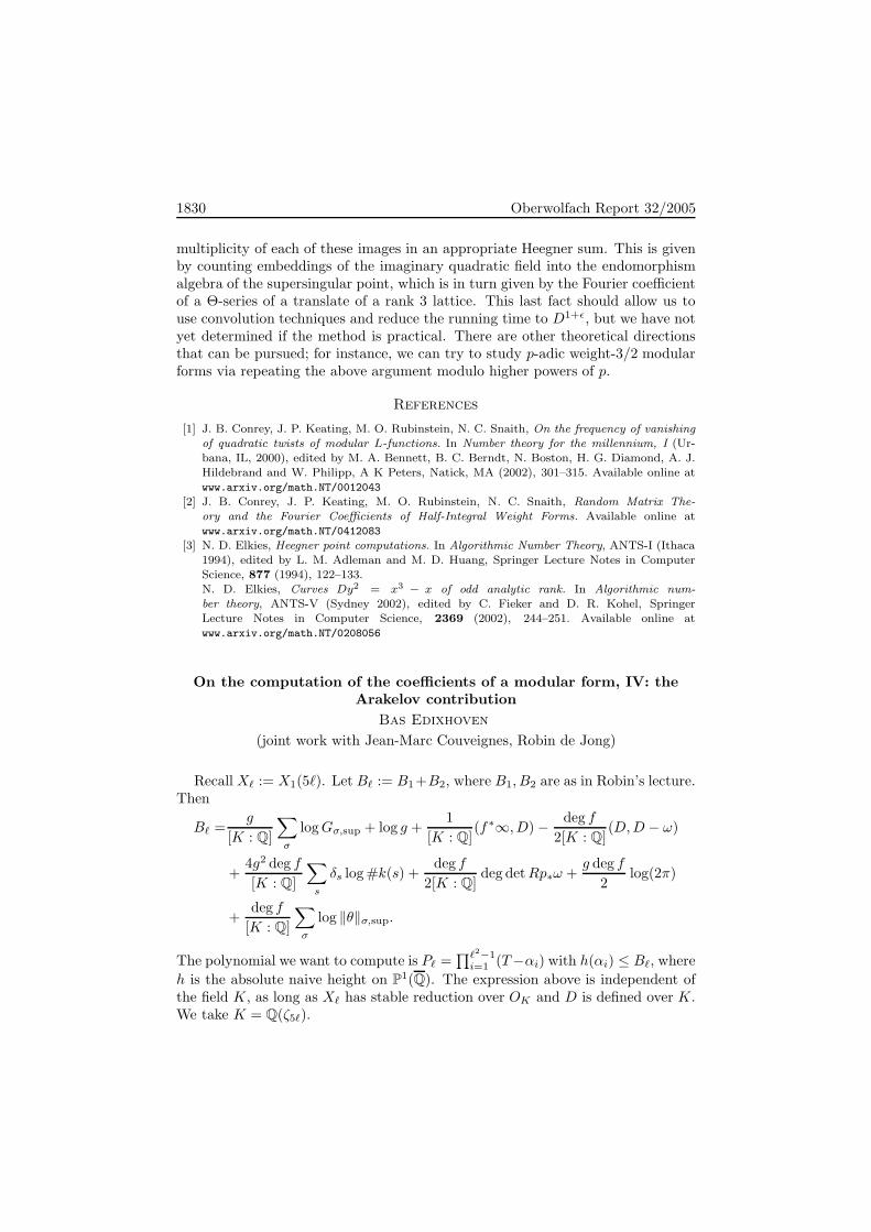
Recall Xℓ := X1(5ℓ). Let Bℓ := B1+B2, where B1, B2 are as in Robin’s lecture.Then
Bℓ =g
[K : Q]
∑
σ
logGσ,sup + log g +1
[K : Q](f∗∞, D) − deg f
2[K : Q](D,D − ω)
+4g2 deg f
[K : Q]
∑
s
δs log #k(s) +deg f
2[K : Q]deg detRp∗ω +
g deg f
2log(2π)
+deg f
[K : Q]
∑
σ
log ‖θ‖σ,sup.
The polynomial we want to compute is Pℓ =∏ℓ2−1
i=1 (T−αi) with h(αi) ≤ Bℓ, where
h is the absolute naive height on P1(Q). The expression above is independent ofthe field K, as long as Xℓ has stable reduction over OK and D is defined over K.We take K = Q(ζ5ℓ).

Explicit Methods in Number Theory 1831
We need to show that there exists c such that Bℓ = O(ℓc). We have
(1) g = O(ℓ2).(2) [K : Q] = 4(ℓ− 1) ≥ ℓ.(3) deg f = O(ℓ2).(4)
∑s δs log #k(s) = O(ℓ log ℓ) + O(l3) = O(l3): contributions only from s|ℓ
and s|5, respectively; there are O(ℓ) supersingular points with s|ℓ, andO(ℓ2) with s|5.
(5) deg detRp∗ω = [K : Q]habs,Falt(Jℓ) = O(ℓ3 log ℓ), where habs,Falt is theabsolute Faltings height. Short sketch: Let vol′ be volume with respect tothe inner product for which the basis ω1, . . . , ωg is orthonormal. Then
hK(Jℓ,K)
[K : Q]≤ hQ(Jℓ,Q) ≤ − log vol
R ⊗ S2(Γ1(5ℓ),Z)
S2(Γ1(5ℓ),Z)= − log vol
R ⊗ T∨
T∨
= log volR ⊗ T
T≤ log vol′
R ⊗ T
T− g
2log π + 2πg
= O(ℓ2 log ℓ),
where the last step comes from bounds on the coefficients an(ωi). Remark:Abbes-Ullmo did X0(squarefree N), but we needed X1.
(6) ∑
σ
log ‖θ‖σ,sup = [K : Q] log ‖θ‖sup = O(ℓℓ4(log ℓ)2ℓ6),
where the ℓ comes from [K : Q], the ℓ4(log ℓ)2 comes from log(det Im τ),and the ℓ6 comes from log(e···|θ|). (As of Tuesday, this no longer dependson Bost’s preprint, but does depend on unpublished work of us!)
(7) ∑
σ
logGσ,sup = [K : Q] logGsup = O(ℓℓ8),
with a non-effective constant. Remark: There is a submitted article byJorgenson and Kramer in which bounds on Green functions are given thatimply that logGsup is bounded uniformly in ℓ.
The bound ℓ8 uses a result of Franz Merkel. Let X be a compactRiemann surface, and µ a positive 2-form (volume form) with
∫X µ = 1.
Let X = U (1) ∪ · · · ∪ U (n) be an open covering, and let z(i) : U (i) → C bea holomorphic function such that z(i)(U (i)) ⊃ D(1) (the closed unit disk).
For 0 ≤ r ≤ 1, let U(i)r := x ∈ U (i) : |z(i)(x)| < r. Fix 0 < r1 < 1 and
suppose
(a)⋃
i U(i)r1 = X
(b) For all i, µ ≤ c1|dz(i)dz(i)| on U(i)1 .
(c) For all i, j, we have
supU
(i)1 ∩U
(j)1
∣∣∣∣dz(i)
dz(j)
∣∣∣∣ ≤M.

1832 Oberwolfach Report 32/2005
Then
logGsup ≤ n(c4 + c9c1 + c7 logM),
where c4, c7, c9 depend only on r1.Application to Xℓ(C). Replace Xℓ by X(5ℓ), together with its action
of SL2(Z/5ℓZ). We can take c1 = O(ℓ3). We have q1/5ℓ = e2πiz/5ℓ. Thereare ≈ ℓ2 cusps. This gives ≈ ℓ2 disks. Small disks: we need O(ℓ4) of them.The choice M = 5 is good.
(8) − 12 (D,D − ω) = O(ℓℓ4ℓ8), where the O(ℓ) comes from [K : Q], the ℓ4
comes from g2, and the ℓ8 comes from the Green functions.(9) (f∗∞, D) = O(ℓℓ4ℓ8) similarly.
Conclusion: Bℓ = O(ℓ14).Also log #R1p∗Lx(D) ≤ O(ℓ15), and the left hand side is at least the sum of
log #k(s) over s such that D′x is not unique over k(s).
Functions, reciprocity and the obstruction to divisors on curves
Samir Siksek
(joint work with Martin Bright)
Let K be a perfect field, C a smooth projective curve over K, and f a non-constant element of the function field K(C). We define
Gf (k) :=∏
P∈C(K)
NormK(P )/K
(K(P )∗)ordP (f).
The product makes sense since all but finitely many of the terms are 1, and theresult is clearly a subgroup of K∗. Our first theorem defines a homomorphismfrom the Picard group Pic(C) to the quotient group K∗/Gf(K) In essence, thismeans that we are doing descent on the Picard group of the curve.
Theorem 2. With notation as above, f induces a unique homomorphism
φ : Pic(C) → K∗/Gf (K)
satisfying the following property: if∑mjQj is a divisor on C whose support is
disjoint from the poles and zeros of f , then the class [∑mjQj ] of this divisor in
Pic(C) is mapped, by φ, to the coset represented by∏
f(Qj)mj
in the group on the right-hand side.
This theorem subsumes many earlier results, by various authors, whereby cer-tain functions on a curve C are shown to induce homomorphisms from the JacobianJ into groups of the form, say, L∗/L∗q, where L is some finite K-algebra, and q issome positive integer.
Now let K be a number field. We denote by IK the idele group of K, andClK := IK/K
∗ the idele class group of K. Again let C be a curve defined over
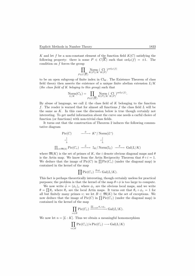
Explicit Methods in Number Theory 1833
K and let f be a non-constant element of the function field K(C) satisfying thefollowing property: there is some P ∈ C(K) such that ordP (f) = ±1. Thecondition on f forces the group
∏
P∈C(K)
NormK(P )/K
( ClK(P )
)ordP (f)
to be an open subgroup of finite index in ClK . The Existence Theorem of classfield theory then asserts the existence of a unique finite abelian extension L/K(the class field of K beloging to this group) such that
NormL/K
(CL) =∏
P∈C(K)
NormK(P )/K
( ClK(P )
)ordP (f).
By abuse of language, we call L the class field of K belonging to the functionf . The reader is warned that for almost all functions f the class field L will bethe same as K. In this case the discussion below is true though certainly notinteresting. To get useful information about the curve one needs a carful choice offunction (or functions) with non-trivial class fields.
It turns out that the construction of Theorem 2 induces the following commu-tative diagram
Pic(C)φ−−−−→ K∗/Norm(L∗)
i
y i
y∏
υ∈M(k) Pic(Cυ)φ−−−−→ IK/Norm(IL)
θ−−−−→ Gal(L/K)
where M(K) is the set of primes of K, the i denote obvious diagonal maps and θis the Artin map. We know from the Artin Reciprocity Theorem that θ i = 1.We deduce that the image of Pic(C) in
∏Pic(Cυ) (under the diagonal map) is
contained in the kernel of the map∏
Pic(Cυ)θφ−−→ Gal(L/K).
This fact is perhaps theoretically interesting, though certainly useless for practicalpurposes; the problem is that the kernel of the map θ φ is too large to compute.
We now write φ = (φυ)υ where φυ are the obvious local maps, and we writeθ =
∏θυ where θυ are the local Artin maps. It turns out that θυ φυ = 1 for
all but finitely many primes υ; we let B ⊂ M(K) be the set of exceptions. Wenow deduce that the image of Pic(C) in
∏Pic(Cυ) (under the diagonal map) is
contained in the kernel of the map
∏
υ∈B
Pic(Cυ)
Q
υ∈B θυφυ−−−−−−−−→ Gal(L/K).
We now let n = [L : K]. Thus we obtain a meaningful homomorphism∏
υ∈B
Pic(Cυ)/nPic(Cυ) −→ Gal(L/K)

1834 Oberwolfach Report 32/2005
whose kernel contains the image of Pic(C)/nPic(C). The good thing is thatPicCυ/nPic(Cυ) is finite and computable and that this allows us to compute thekernel.
Now an element of Pic(Cυ)/nPic(Cυ) does not have a well-defined degree, butit does have a well-defined degree modulo n. If 0 ≤ r < n, we denote by
(Pic(Cυ)/nPic(Cυ))r
to be the subset of elements that have degree r modulo n. This subset containsthe images of
Picr(C), Picr+n(C), Picr+2n(C), . . .
in Pic(Cυ)/nPic(Cυ). We immediately obtain the following theorem.
Theorem 3. Consider the induced map
∏
υ∈B
(Pic(Cυ)/nPic(Cυ))r −→ Gal(L/K).
The subset of elements of the set on the left-hand side sent to 1 under this mapis finite. If this subset is empty then Picr(C), Picr+n(C), Picr+2n(C), . . . are allempty.
Finally we give an example to show that the above scenario is realistic.
Example. Let C/Q be the genus 1 curve given by
C : y2 = −727x4 − 104x3 + 92x2 + 4x− 4.
The curve C has points everywhere locally. We would like to show that C doesnot have any rational points. Take
f =x+ 16/53
x;
in this case it is possible to show that L = Q(i). We identify Gal(L/K) withµ2 = 1,−1.
Primes Basis for Pic(Cp)/2 Pic(Cp) φ(P ) (θp φ)(P )
p = ∞ P0 = (−0.3018 . . . , 0.0003 . . .) −0.00028 −1
p = 2P0 = (2−1, 2−2 + 1 + 2 + · · · ) 1 + 25 + · · · 1P1 = (2−4 + · · · , 2−8 + · · · ) 1 + 28 + · · · 1
We see that the “Kernel” of (∏
p Pic(Cp)/2 Pic(Cp))1 → 1,−1 is empty. Thus
C(Q) = ∅.

Explicit Methods in Number Theory 1835
References
[1] S. Siksek, Sieving for rational points on hyperelliptic curves, Math. Comp. 70 (2000), 1661–1674.
[2] S. Siksek, Descent on Picard groups using functions on curves, Bull. Austral. Math. Soc.66 (2002), 119–124.
[3] S. Siksek and A. Skorobogatov, On a Shimura curve that is a counterexample to the Hasseprinciple, Bull. London Math. Soc. 35 (2003), 409–414.
[4] M. Bright and S. Siksek, Functions, reciprocity and the obstruction to divisors on curves,in preparation.
Integral points on congruent number curves
Michael A. Bennett
(joint work with P.G. Walsh)
If N is a positive integer, then N is a congruent number, that is, there exists aright triangle with rational sides and area N , precisely when the elliptic curve
EN : y2 = x3 −N2x
has infinitely many rational points. In this talk, we address the question of whethercurves of the shape EN possess integral points of infinite order, provided we knowthey have rational points with this property. We will concentrate on the casewhere N = 2apb for a and b nonzero integers and p an odd prime. Since EN isrationally isomorphic to Em2N for each nonzero integer m, and since both E1 andE2 have rank 0 over Q, we may suppose, without loss of generality, that b is odd.
¿From now on, we will fix p to be an odd prime number, and a and b to benonnegative integers. We are interested in describing the integer solutions (x, y),with, say, y > 0 to the Diophantine equation.
(5) y2 = x(x+ 2apb)(x − 2apb).
A solution (x, y) (with y > 0) to (5) will be called primitive if either
minν2(x), a ≥ 2 or minνp(x), b ≥ 2.
¿From the above remarks, clearly it is enough to determine all primitive integersolutions. These correspond to the S-integral points on Ep and E2p, where S =2, p.
Our main result is that all solutions are as follows. First, we have the followingsporadic solutions; in each case b = 1.
(6)
p a x p a x p a x p a x3 1 −3 3 3 25 7 3 −7 29 0 2843393 1 −2 5 0 −4 7 4 −63 41 6 420253 1 12 5 0 45 11 1 21783 1 18 5 2 25 17 5 8333 1 294 7 1 112 17 7 16337
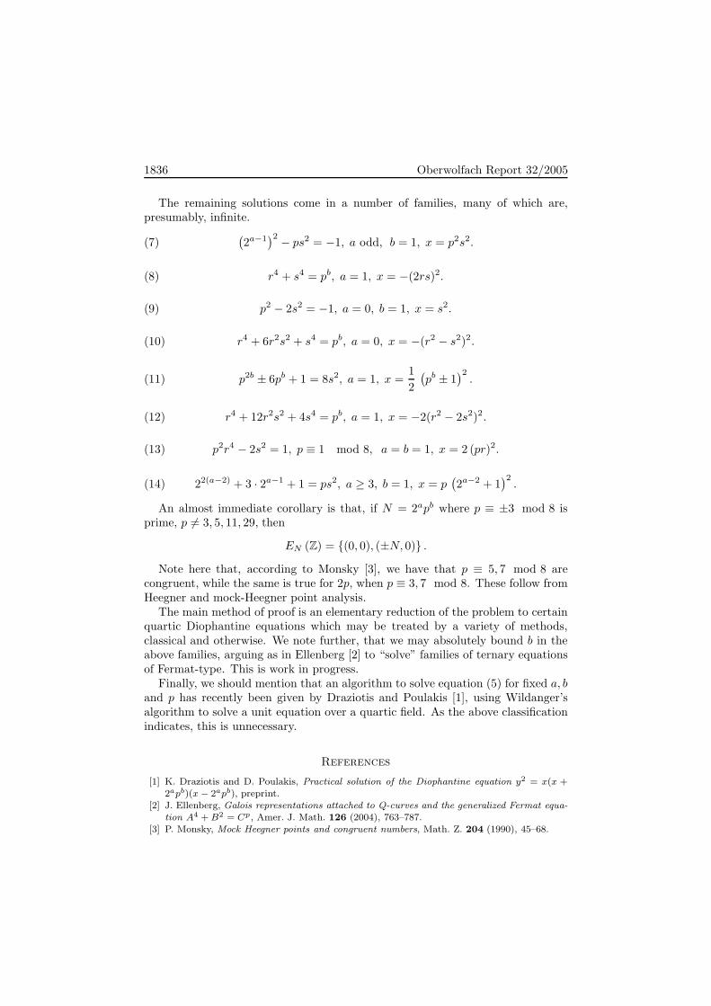
1836 Oberwolfach Report 32/2005
The remaining solutions come in a number of families, many of which are,presumably, infinite.
(7)(2a−1
)2 − ps2 = −1, a odd, b = 1, x = p2s2.
(8) r4 + s4 = pb, a = 1, x = −(2rs)2.
(9) p2 − 2s2 = −1, a = 0, b = 1, x = s2.
(10) r4 + 6r2s2 + s4 = pb, a = 0, x = −(r2 − s2)2.
(11) p2b ± 6pb + 1 = 8s2, a = 1, x =1
2
(pb ± 1
)2.
(12) r4 + 12r2s2 + 4s4 = pb, a = 1, x = −2(r2 − 2s2)2.
(13) p2r4 − 2s2 = 1, p ≡ 1 mod 8, a = b = 1, x = 2 (pr)2.
(14) 22(a−2) + 3 · 2a−1 + 1 = ps2, a ≥ 3, b = 1, x = p(2a−2 + 1
)2.
An almost immediate corollary is that, if N = 2apb where p ≡ ±3 mod 8 isprime, p 6= 3, 5, 11, 29, then
EN (Z) = (0, 0), (±N, 0) .
Note here that, according to Monsky [3], we have that p ≡ 5, 7 mod 8 arecongruent, while the same is true for 2p, when p ≡ 3, 7 mod 8. These follow fromHeegner and mock-Heegner point analysis.
The main method of proof is an elementary reduction of the problem to certainquartic Diophantine equations which may be treated by a variety of methods,classical and otherwise. We note further, that we may absolutely bound b in theabove families, arguing as in Ellenberg [2] to “solve” families of ternary equationsof Fermat-type. This is work in progress.
Finally, we should mention that an algorithm to solve equation (5) for fixed a, band p has recently been given by Draziotis and Poulakis [1], using Wildanger’salgorithm to solve a unit equation over a quartic field. As the above classificationindicates, this is unnecessary.
References
[1] K. Draziotis and D. Poulakis, Practical solution of the Diophantine equation y2 = x(x +2apb)(x − 2apb), preprint.
[2] J. Ellenberg, Galois representations attached to Q-curves and the generalized Fermat equa-tion A4 + B2 = Cp, Amer. J. Math. 126 (2004), 763–787.
[3] P. Monsky, Mock Heegner points and congruent numbers, Math. Z. 204 (1990), 45–68.

Explicit Methods in Number Theory 1837
Local Galois module structure for Artin-Schreier extensions ofdegree p
Bart de Smit
(joint work with Lara Thomas)
Let L/K be a Galois extension of local fields with [L : K] = p = char(K). Let Gbe the Galois group and A ⊂ B the extension of valuation rings. By the normalbasis theorem, L is free of rank 1 as a module over the group ring K[G]. Thevaluation ring B is free of rank 1 over A[G] if and only if L/K is unramified.Let us assume that L/K is totally ramified, i.e., that the ramification index is p.Let k be the resdue field of A, which is also the residue field of B. We let r bethe ramification number of L/K, so the filtration of G with ramification groupssatisfies Gr 6= Gr+1.
The multiplier ring of B, or the associated order of B, is defined as R = x ∈K[G] : xB ⊂ B. Note that R is the endomorphism ring of B as an A[G]-module. It is a complete local ring, which is free of rank p as an A-module. Welet e = dimk(mR/m
2R) be the embedding dimension of R, and we will show that
it is tightly related to the number of R-module generators of B.We first present a slight strengthening and an independent proof of a result of
Aiba and Lettl [1, 4], whose characteristic 0 analog is given in [2]:
B is a free R-module ⇐⇒ e ≤ 3 ⇐⇒ s | p− 1.
Here s is the remainder of r when we divide by p, which satisfies 0 < s < p.Our second result says that when s 6= p− 1 the embedding dimension e of R is
exactly 2d+ 1, where d is the minimal number of R-module generators of B.The proof uses the combinatorics of balanced sequences, which turns out to be
encoded by the Hirzebruch continued fraction [3]. One can rewrite this in termsof the usual continued fraction [5] and obtain the following: If
−r/p = x0 +1
x1 +1
.. .
. . .
xn−1 +1
xn
with x0, . . . , xn ∈ Z, and x1, . . . , xn−1 ≥ 1 and xn ≥ 2, then
d =∑
i<n odd
xi.
This also gives rise to a polynomial time algorithm that given p and r computes dand e.
References
[1] A. Aiba, Artin-Schreier extensions and Galois module structure. J. Number Theory 102
(2003), 118–124.

1838 Oberwolfach Report 32/2005
[2] F. Bertrandias and M.-J. Ferton, Sur l’anneau des entiers d’une extension cyclique de degrepremier d’un corps local, C. R. Acad. Sci. Paris Ser. A-B 274 (1972), A1330–A1333.
[3] F. Hirzebruch, Uber vierdimensionale Riemannsche Fl”achen mehrdeutiger analytischerFunctionen von zwei komplexen Veranderlichen, Math. Ann. 126 (1953), 1–22.
[4] G. Lettl, Note on a theorem of A. Aiba, to appear in: J. Number Theory.[5] D.B. Zagier, Zetafunctionen und quadratische Korper, Springer-Verlag Hochschultext, 1981.
Hecke operators and class numbers
Nicole Raulf
Let K be an imaginary quadratic number field of class number one and denote itsring of integers by O and the set of units of O by O∗. Furthermore, let q = [a, b, c]denote a primitive quadratic form whose coefficients belong to O and whose dis-criminant is an element of Ω := d ∈ O \ 0 : d ≡ x2 mod 4, d no square.Remember that primitive means that the ideal generated by the coefficients of q isequal to O. For d ∈ Ω let hd be the class number of primitive quadratic forms, i. e.imposing the usual equivalence relation on primitive quadratic forms, hd is thenumber of inequivalent primitive quadratic forms of discriminant d. Furthermore,for d ∈ Ω consider Pell’s equation t2 − du2 = 4, t, u ∈ O. ǫd is the fundamentalsolution of this equation and ζd is a root of unity of maximal order which can be
written in the form ζd = t1+u1
√d
2 , t21 − du21 = 4. If we write ζd = eπi/md , then
md ∈ 1, 2, 3. Having introduced all notations, we can now state the theorem.
Theorem 1. For v ∈ O \ 0 we have:
∑
|du2|≤x
hd log |ǫd|md
∼
1
4|v|2∑
d∈O/O∗,d|v
|d|2
x2 as x→ ∞
where we sum over all d ∈ Ω and u ∈ O/O∗ such that |du2| ≤ x and ∃t ∈ O so
that t2 − du2 = 4v and | t+u√
d2√
v| 6= 1.
This mean value theorem is proved with the help of Hecke operators. The Heckeoperators we work with act on PSL2(O) - invariant functions on the upper half -space H3. The upper half - space H3 is equipped with the hyperbolic metric andthe corresponding Laplace operator is denoted by ∆. When trying to express thetrace of the Hecke operator Tv, v ∈ O \ 0, on a fixed eigenspace of −∆ in termsof hd and log |ǫd|, the following L - series appears:
Lv(s) :=∑
d∈Ω
∑
u
hd log |ǫd|md|du2|s ,
where the u - summation extends over all u ∈ O \ O∗ such that ∃t ∈ O with
the property t2 − du2 = 4v and | t+u√
d2√
v| 6= 1. The discussion shows that Lv(s)
converges absolutely for Re s > 2 and has an analytic continuation for Re s ≥ 3/2

Explicit Methods in Number Theory 1839
except for a simple pole at s = 2. Hence a Tauberian theorem implies the theoremstated above.
References
[1] N. Raulf, Traces of Hecke Operators Acting on Three - Dimensional Hyperbolic Space, Dis-sertation Munster (2004).
[2] N. Raulf, Traces of Hecke Operators acting on Three - Dimensional Hyperbolic Space, toappear in J. Reine Angew. Math.
Class invariants in a non-archimedean setting
Reinier Broker
The theory of complex multiplication provides us with a means of explicitly com-puting the Hilbert class field H = H(K) of an imaginary quadratic number fieldK. Let D = disc(K) < 0 be the discriminant of K and define
EllD(C) = E/C |E is an elliptic curve over C with End(E) ∼= OK∼=as the finite set of elliptic curves E/C with endomorphism ring isomorphic to thering of integers OK of K. We have the following theorem, usually called the firstmain theorem of complex multiplication.
Theorem. For [E] ∈EllD(C) we have H = K(j(E)). Moreover the polynomial,
fD =∏
[E]∈EllD(C)
(X − j(E)) ∈ Z[X ]
has integer coefficients.
The polynomial fD is usually called the Hilbert class polynomial. We are interestedin efficiently computing this polynomial.
The degree of fD equals the class number of K and hence grows exponentiallyin log |D|. Since any algorithm computing fD has to write down the answer, thisshows that there can’t exist a polynomial time algorithm that computes fD.
The classical algorithm of evaluating the modular function j : H → C in pointsτ ∈ H corresponding to the ideal classes of the class group Cl(O) can be improvedin two ways. Firstly, one can work in a non-archimedean setting as explained in[1]. This avoids the problem of rounding errors that might occur when expandingthe product
fD =∏
[E]∈EllD(C)
(X − j(E)) ∈ Z[X ].
The second improvement is inspired by the fact that even for moderately smalldiscriminants D, the coefficients of fD are already huge. As example, for D = −31we get coefficients of 16 digits. We can save a constant factor in the size of thecoefficients by using other (‘smaller’) functions than the j-function.
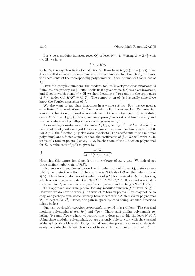
1840 Oberwolfach Report 32/2005
Let f be a modular function (over Q) of level N ≥ 1. Writing O = Z[τ ] withτ ∈ H, we have
f(τ) ∈ HN ,
with HN the ray class field of conductor N . If we have K(f(τ)) = K(j(τ)), thenf(τ) is called a class invariant . We want to use ‘smaller’ function than j, becausethe coefficients of the corresponding polynomial will then be smaller than those offD.
Over the complex numbers, the modern tool to investigate class invariants isShimura’s reciprocity law (1970). It tells us if a given value f(τ) is a class invariant,and if so, in which points τ ′ ∈ H we should evaluate f to compute the conjugatesof f(τ) under Gal(H/K) ∼= Cl(O). The computation of f(τ) is easily done if weknow the Fourier expansion of f .
We also want to use class invariants in a p-adic setting. For this we need asubstitute of the evaluation of a function via its Fourier expansion. We note thata modular function f of level N is an element of the function field of the modularcurve X(N) over Q(ζN ). Hence, we can express f as a rational function in j andthe x-coordinates of an elliptic curve with j-invariant j.
As example, consider an elliptic curve E/Qp given by Y 2 = X3 + aX + b. Thecube root γ2 of j with integral Fourier expansion is a modular function of level 3.For 3 6 |D, the function γ2 yields class invariants. The coefficients of the minimalpolynomial are a factor 3 smaller than the coefficients of fD. We will write γ2 interms of 3-torsion points. Let c1, . . . , c4 be the roots of the 3-division polynomialfor E. A cube root of j(E) is given by
(1)−48a
2a− 3(c1c2 + c3c4).
Note that this expression depends on an ordering of c1, . . . , c4. We indeed getthree distinct cube roots of j(E).
Expression (1) enables us to work with cube roots of j over Qp. We can ex-plicitly compute the action of the coprime to 3 ideals of O on the cube roots ofj(E). This allows to decide which cube root of j(E) is contained in H , by checkingwhich one is invariant under Gal(H3/H) ∼= (O/3O)∗/O∗. If we find one that iscontained in H , we can also compute its conjugates under Gal(H/K) ∼= Cl(O).
This approach works in general for any modular function f of level N ≥ 1.However, we do have to write f in terms of N -torsion points. This may not be soeasy, and perhaps even worse, we may have to factor the N -th division polynomialΨN of degree O(N2). Hence, the gain in speed by considering ‘smaller’ functionsmight be lost.
One can work with modular polynomials to avoid this problem. The classicalmodular polynomial relates j(τ) and j(pτ). There exist similar polynomials re-lating f(τ) and f(pτ), where we require that p does not divide the level N of f .Using these modular polynomials, we are currently able to work with the classicalWeber-f function of level 48. Using normal computer power, we can now relativelyeasily compute the Hilbert class field of fields with discriminant up to −1010.

Explicit Methods in Number Theory 1841
References
[1] Couveignes, J.-M. and Henocq, T.: Action of modular correspondences around CM pointsin Algorithmic Number Theory Symposium V, Lecture Notes in Computer Science 2369,(2002), 234–243.
Explicit computations on the Manin conjectures
Ronald van Luijk
Even though finding the set of rational points on a curve could be very hard,once the set is known, it is easy to describe. If it is not a finite set, then thegenus g of the curve is at most 1. In case g = 0 we can give a parametrizationof the curve and in case g = 1 the set naturally carries the structure of a finitelygenerated group, for which we can give a set of generators.
For a higher-dimensional variety X ⊂ Pn over a number field k it is not soeasy to describe the set X(k) of rational points. To this extend we define acounting function NU for any open subset U of X , based on a height functionH : Pn(k) → R>0. For k = Q the height function is defined by
H(x) = maxi
(|xi|) when
x = [x0 : x1 : . . . : xn]xi ∈ Zgcd(x0, . . . , xn) = 1
and for higher degree number fields we use the standard generalization. Thecounting function NU : R>0 → Z≥0 is defined by
NU (B) = #x ∈ U(k) : H(x) ≤ B.We want to understand the asymptotic behavior of NU as B tends to infinity. Forsome easy to understand varieties X we find that there exists an open subset Uof X such that we have
NU (B) ≈ CBa(logB)b,
where C is some constant, a is a number such that the canonical sheaf ωX isisomorphic to O(−a), and b+1 is the rank of the Neron-Severi group NS(X) of X .The conjecture of Batyrev and Manin states that if the canonical divisor ofX ⊂ Pn
k
is isomorphic to O(−a) for some a > 0, then there exists a finite field extension lof k, an open subset U ⊂ X , and a constant C such that with b = rankNS(Xl)− 1we have
(15) NUl(B) ≈ CBa(logB)b.
Even though Batyrev and Tschinkel found a counter example to this conjecturein dimension 5, there is a lot of evidence for the case of dimension 2. We look atthe degenerate case of a = 0, namely those of trivial canonical sheaf, in particularthe case of K3 surfaces. Martin Bright has computed NX(B) for many diagonalquartic surfaces X and B up to 106. Especially those with low Neron-Severi rank
1842 Oberwolfach Report 32/2005
tend to have too few points with low height to extrapolate from. We use thequartic surface in P3 given by
w(x3 + y3 + z3 + x2z + xw2) = 3x2y2 − 4x2yz + x2z2 + xy2z + xyz2 − y2z2,
which has Neron-Severi rank 1 even over the algebraic closure. With a programwritten by Michael Stoll, based on a variation of an algorithm by Noam Elkies,we computed all points of height at most 15000, of which there turn out to be 46that do not lie on the two rational curves given by xw = 0. Let U be the opensubset outside these two rational curves. Then NU (B) appears to grow like logB,rather than being bounded as one would conclude from (15). One explanationwould be that the factor Ba in (15) comes from an integral
∫Ba−1db, which for
a = 0 yields logB instead of Ba. This potentially leads to an extension of theManin conjecture to K3 surfaces.
[1] V. Batyrev and Y. Manin, Sur le nombre des points rationnel de hauteurborne des varietes algebriques, Math. Ann. 286 (1990), no. 1–3, pp.27–43.
[2] E. Peyre, Counting points on varieties using universal torsors, Arith-metic of Higher-Dimensional Algebraic Varieties, eds. B. Poonen and Y.Tschinkel, Prog. in Math. 226 (2004).
[3] R. van Luijk, K3 surfaces with Picard number one and infinitely manyrational points, preprint.
On the computation of the coefficients of a modular form, V:computational aspects
Jean-Marc Couveignes
This talk is the continuation of the ones by Johan Bosman, Bas Edixhovenand Robin de Jong. I will address the problem of computing torsion divisors, withprescribed Hecke action, on modular curves (e.g. divisor classes in the linear spaceVℓ image of the modulo ℓ Galois representation ρℓ attached to the Ramanujan τ -function). We need algorithms that can be proven to be polynomial time.
We have three possible strategies for doing this. We first may calculate complexapproximations for the divisors we are interested in. The difficulty is then to showthat we can perform efficient and stable numerical computations in the jacobian ofmodular curves, in deterministic polynomial time in both the level and the requiredaccuracy. These computations should include addition/subtraction in the jacobianand the explicit solution to the inverse Jacobi problem. This has been done in [1]for the curves X0(p) when p tends to infinity. Adapting these methods to thecase of X1(5p) would suffice for the computation of the Ramanujan τ function.A second possibility would be to fix an auxiliary small prime p and compute thetorsion divisors we are interested in modulo p. We may then Hensel lift thesedivisors and obtain good p-adic approximations. The third method which I wantto present in this talk computes the divisors modulo many different small primesp and then recovers the actual divisors in characteristic zero by Chinese remainder

Explicit Methods in Number Theory 1843
theorem. It is slightly less efficient than the previous one. But it is simpler toexplain.
It should be stressed that the efficiency of all these methods depends on thebound on the height of torsion divisors that was presented by Edixhoven and deJong. Indeed, this bound controls the accuracy (resp. the number of auxiliaryprimes p) we need.
As far as the complex analytic method is concerned, the bound is also necessaryto prove the numerical stability of the algorithm. As far as the modulo p method isconcerned, there could be some instability also : namely if one of the divisors we arelooking for becomes special when reduced modulo p. The bound by Edixhoven andde Jong shows that the number of such bad primes p is bounded by a polynomialin ℓ.
The description and proof of the algorithm goes in four steps.
(1) define and compute some explicit model for the curve X1(ℓ) or some smallcovering Xℓ of it.
(2) provide enough information on this curve (in particular its singularities) tobe able to compute in its jacobian using what is known as the Brill-Noetheralgorithm.
(3) construct elements in the ℓ-Sylow subgroup of the group of Fq-points ofthe jacobian of X1(ℓ).
(4) using Hecke operators, construct a point in Vℓ = ∩n≥2 Ker(Tn − τ(n)).
We now detail these four steps.(1) — The modular curve X(2)1(ℓ)
Let ℓ ≥ 5 be a prime. We set dℓ = ℓ2−14 and mℓ = ℓ−1
2 . We denote byXℓ = X(2)1(ℓ) the moduli of elliptic curves with full 2-torsion plus one non-trivialℓ-torsion point.
Let λ be an indeterminate and form the Legendre elliptic curve with equationy2 = x(x− 1)(x− λ). Call Tℓ(λ, x) the ℓ-division polynomial of this curve. It has
degree 2dℓ = ℓ2−12 in x and dℓ in λ. We denote by Tℓ(Λ, X, Y ) = Tℓ(
ΛY ,
XY )Y 2d the
associated homogeneous polynomial and call Cℓ ⊂ P2 the corresponding projectivecurve. This is a singular plane model for Xℓ.
The morphism φ : Xℓ → X1(ℓ) corresponding to forgetting the 2-torsion struc-ture is Galois with group S3. The six corresponding automorphisms extend to P2
and Cℓ in a way compatible with the maps Xℓ → Cℓ and Cℓ ⊂ P2. The group isgenerated by the two transpositions τ(0,∞) and τ(0,1) defined in homogeneous coor-dinates by τ(0,∞) : [Λ, X, Y ] → [Y,X,Λ] and τ(0,1) : [Λ, X, Y ] → [Y −Λ, Y −X,Y ].
(2) — Singularities on Cℓ
The only possible singularities of Cℓ lie on one of the three lines with equationsΛ = 0, Y = 0 and Λ−Y = 0. We study the branches at infinity on Cℓ through theassociated Tate’s elliptic curves and deduce the 2dℓ roots of Tℓ(λ, x) in the fieldQλ−1 of Puiseux series in λ−1. We introduce Tate’s q-parameter, definedimplicitly by j = 1
q + 744 + · · · . For a and b integers such that either b = 0 and
1 ≤ a ≤ ℓ−12 or 1 ≤ b ≤ ℓ−1
2 and 0 ≤ a ≤ ℓ−1 we consider the ℓ-torsion point ζaℓ q
bℓ

1844 Oberwolfach Report 32/2005
on the Tate curve with parameter q and call xa,b the corresponding expansion of
x as a series in λ−1ℓ . We find
xa,b = −4ζaℓ 2
−8bℓ λ1− 2b
ℓ +O(λ1− 2b+1ℓ )
if b 6= 0 and xa,0 =−4ζa
ℓ
(1−ζaℓ )2 λ + O(1). We call Σ∞ = [1, 0, 0] the unique singular
point at infinity and for every 1 ≤ b ≤ ℓ−12 we call σ∞,b the point above Σ∞ on Xℓ
associated to the orbit x0,b, x1,b, · · · , xℓ−1,b for the inertia group. We call µ∞,a
the point on Xℓ corresponding to the expansion xa,0. The ramification index ofthe covering map λ : Xℓ → X(2) is ℓ at σ∞,b and 1 at µ∞,a.
The genus of Xℓ is gℓ = (ℓ−3)2
4 = (mℓ − 1)2. The arithmetic genus of Cℓ is
ga = (m2ℓ + mℓ − 1)(2m2
ℓ + 2mℓ − 1). We now compute the conductor of Cℓ.Locally at Σ∞ the curve Cℓ consists of mℓ branches (one for each place σ∞,b) that
are cusps with equations(
XΛ
)ℓ= −22ℓ−8b
(YΛ
)2b+ · · · . The conductor of this later
cusp is σ∞,b times (ℓ− 1)(2b− 1) which is the next integer to the last gap of theadditive semigroup generated by ℓ and 2b. The conductor of the full singularityΣ∞ is now given by Gorenstein’s formula [5, Theorem 2] and is
∑
1≤b≤mℓ
b(4m2ℓ + 4mℓ − 1) − 2mℓ − (2mℓ + 1)b2 · σ∞,b.
The full conductor Cℓ is the sum of this plus the two corresponding terms to theisomorphic singularities Σ0 and Σ1. Some authors call it the adjunction divisor.
The degree deg(Cℓ) of Cℓ is 2mℓ(2m3ℓ + 4m2
ℓ − 2mℓ − 1). So we have δ(Cℓ) =mℓ(2m
3ℓ + 4m2
ℓ − 2mℓ − 1) and we check that ga = gℓ + δ(Cℓ).(2’) — The Brill-Noether algorithmLet p 6∈ 2, 3, ℓ be a prime. Le Cp be the field of p-adics and Fp its residue
field. We embed Q in Cp and also in C. In particular ζℓ = exp(2iπℓ ) and 2
1ℓ are
well defined as p-adic numbers.We set hℓ = 3mℓ(mℓ +1). Let Shℓ = H0(P2,OP2(hℓ)) the linear space of degree
hℓ homogeneous polynomials in Λ, X , and Y . Let Hhℓ be the space of hℓ-formson Xℓ. If mℓ ≥ 8 then the dimension of Hhℓ(Cℓ) is greater than 2gℓ and therestriction map ρ : Shℓ → Hhℓ contains Hhℓ(Cℓ) according to the residue theorem.So we have a description of Hhℓ(Cℓ) as a subspace of Shℓ .
A place p of the field Fq(Xℓ) is represented in the following way. Le P be an
Fq-point on Xℓ above p. If P lies on one of the lines with equations Λ = 0, Y = 0and Λ−Y = 0 then it is one of the σ’s or one of the µ’s and we already know howto call it.
Otherwise, P is a smooth point and may be regarded as a point on the affinepart of the plane curve Cℓ. Let rp be the degree of p which is also the degreeof Fq(P ) over Fq. The point P can be given by its affine coordinates λ andx. We call rλ the degree of Fq(λ(P )) over Fq and set rx/λ = rp/rλ. We callFp(λ) ∈ Fq[λ] the unitary, irreducible polynomial with degree rλ that cancelsλ(P ). We call Gp(λ, x) ∈ Fq[λ, x] = Fq[λ][x] the unique polynomial with degree

Explicit Methods in Number Theory 1845
rx/λ in x and degree < rλ in λ such that the coefficient of xrx/λ is 1 ∈ Fq[λ] andGp(λ(P ), x(P )) = 0.
So we can represent forms and divisors on our modular curve. For every formin Hhℓ(Cℓ) we can compute its divisor. And given a divisor, we can compute thesubspace of Hhℓ(Cℓ) consisting of forms that vanish at this divisor. This is enoughto compute in the jacobian Jℓ of Xℓ.
(3) — The ℓ-Sylow subgroup of J1(ℓ)(Fq)Recall there is a covering map φ : Xℓ → X1(ℓ) corresponding to forgetting the 2-
torsion structure. This induces two morphisms φ∗ : J1(ℓ) → Jℓ and φ∗ : Jℓ → J1(ℓ)such that φ∗ φ∗ = [6] on J1(ℓ).
We denote by Jℓ ⊂ Jℓ the image of ν = φ∗ φ∗. This is a subvariety of Jℓ
isogenous to J1(ℓ). The restriction of ν to Jℓ is multiplication by 6. The mapsφ∗ and φ∗ induce Galois equivariant bijections between the N -torsion subgroupsJ1(ℓ)[N ] and Jℓ[N ] for every prime to 6 integer N .
For any finite field k and abelian variety A/k and prime integer n, we denoteby A[n∞](k) the n-Sylow subgroup of A(k). We note Nq the number of Fq-pointsin J1(ℓ)(Fq) and set Nq = LqMq where Mq is prime to ℓ and Lq is a power of ℓ.We check the map [Mq] ν = φ∗ Mq φ∗ : Jℓ(Fq) → Jℓ[ℓ
∞](Fq) is surjective.By Eichler-Shimura and results of Manin, Shokurov, Merel, Cremona, [6, 7, 2,
4], for q = pk a power of a prime p 6= ℓ, the number of Fq-rational points on J1(ℓ)is computed in time polynomial in ℓ, p, and k.
Starting from elements in Jℓ(Fq) and applying the operator [Mq] φ∗ φ∗, weconstruct elements in the group Jℓ[ℓ
∞](Fq).(4) — projecting into the Ramanujan subgroup
We choose an integer 6 such that 66 is congruent to 1 modulo Lq. We set
Tn = [6]φ∗ Tn φ∗ and notice that Tn φ∗ = φ∗ Tn on J1(ℓ)[ℓ∞]. This way, the
map φ∗ : J1(ℓ)[ℓ∞](Fq) → Jℓ[ℓ
∞](Fq) becomes a bijection of Hecke modules. Theforecoming calculations are more naturally described in J1(ℓ)[ℓ
∞](Fq) but theywill be performed in Jℓ[ℓ
∞](Fq).We call A the algebra of endomorphisms of J1(ℓ)/Fp generated by the operators
Tn for all prime integers n. We set B = A[Fp] where Fp is the p-Frobenius operator.We assume the polynomial X2 − τ(p)X + p11 splits modulo ℓ and call a and b
the two roots in Zℓ which we assume to be distinct modulo ℓ. The method can beeasily adapted in the inert case.
We call V aℓ ⊂ Vℓ the eigenspace associated to a and V b
ℓ the eigenspace associatedto b. We denote ma the maximal ideal in B generated by ℓ, the Tn−τ(n) and Fp−a.For every integer n ≥ 2 we call An(X) ∈ Z[X ] the characteristic polynomial of Tn
acting on modular forms of weight 2 for Γ1(ℓ). We factor An(X) = bn(X)(X −τ(n))en in Fℓ[X ] with bn(X) unitary and bn(τ(n)) 6= 0 ∈ Fℓ. We set q = pka whereka > 0 is an integer that kills a in (Z/ℓZ)∗ and observe that V a
ℓ = V aℓ (Fq). The
ℓ-Sylow subgroup J1(ℓ)[ℓ∞](Fq) of J1(ℓ)(Fq) is contained in J1(ℓ)[Lq](Fq). We set
Lq = ℓwq . The polynomial factorization An(X) = bn(X)(X − τ(n))en modulo ℓlifts modulo Lq as An(X) = Bn(X)Cn(X).
1846 Oberwolfach Report 32/2005
We call Πa the composite map of (Fp − [b mod Lq])2g(X1(ℓ)) and all Bn(Tn) for
all n primes such that 2 ≤ n ≤ ℓ2. The image of J1(ℓ)[ℓ∞](Fq) by Πa contains
V aℓ = J1(ℓ)[ma] and is killed by m
2wqg(X1(ℓ))a .
Given a non-zero element x in the image of J1(ℓ)[ℓ∞](Fq) by Πa, we can test
whether it is killed by ma by applying to it all the generators ℓ and Tn − τ(n) forn ≤ ℓ2. If we always obtain zero this shows that x is in V a
ℓ . Otherwise we producesome non zero element in mx and we replace x by this element and iterate. Thisprocess stops after at most 2g(X1(ℓ))wq steps and produces a non-zero element xin V a
ℓ . We proceed in a similar way with V bℓ and find a generating set for Vℓ.
References
[1] Jean-Marc Couveignes. Jacobiens, jacobiennes et stabilite numerique. http://www.univ-tlse2.fr/grimm/couveignes, 2004.
[2] J. E. Cremona. Algorithms for modular elliptic curves. Cambridge University Press, 1997.[3] Sebastiaan Edixhoven. On computing coefficients of modular forms. Talk at MSRI,
http://www.math.leidenuniv.nl/∼edix/public html rennes/talks/msridec2000.html, 2000.[4] Gerhard Frey and Michael Muller. Arithmetic of modular curves and applications. In On
Artin’s conjecture for odd 2-dimensional representations, number 1585 in Lecture Notes inMath. Springer, 1994.
[5] D. Gorenstein. An arithmetic theory of adjoint plane curves. Trans. Amer. Math. Soc.,72:414–436, 1952.
[6] Yuri Manin. Parabolic points and zeta function of modular curves. Math. USSR Izvestija,6(1):19–64, 1972.
[7] Loıc Merel. Universal fourier expansions of modular forms. In On Artin’s conjecture for odd2-dimensional representations, number 1585 in Lecture Notes in Math. Springer, 1994.
Computations in non-commutative Iwasawa theory of elliptic curves
Tim Dokchitser
(joint work with Vladimir Dokchitser)
Recently a “Main Conjecture of non-commutative Iwasawa theory” has been for-mulated by J. Coates, T. Fukaya, K. Kato, R. Sujatha and O. Venjakob [1]. Take anumber field F , an elliptic curve E/F , and an extension F∞/F whose Galois groupΓ is a compact p-adic Lie group, not necessarily commutative. With some restric-tions on F,Γ and E, the conjecture predicts a relation between the non-abelianEuler characteristic (defined by the authors) of twists E ⊗ τ of E in F∞/F , andspecial values of L-functions L(E, τ, s)|s=1. We want to provide some of the firstnumerical evidence in favour of their conjecture.
Namely, take F = Q, Fn = Q(µpn , pn√m) and F∞ =
⋃n Fn. Then F∞/F is
Galois and its Galois group is possibly the simplest non-commutative compactp-adic Lie group,
Γ = Gal(F∞/F ) ∼=( ∗ ∗
0 1
)∈ GL2(Zp)
.
Explicit Methods in Number Theory 1847
This Lie group is 2-dimensional, and its first layer Gal(F1/Q) is of order p(p− 1);it is somewhat similar to a dihedral group of order 2p. It is not hard to see that
The regular representation of Gal(F1/Q) ∼= σ ⊕ ρp−1 .
Here σ is the regular representation of Gal(Q(µp)/Q and ρ is a sum of p− 1 one-dimensional characters; ρ is irreducible of dimension p − 1. The representationsρ and σ arise naturally when one describes L-functions of E over the subfields ofF1, for instance
L(E/F1, s) = L(E, σ, s)L(E, ρ, s)p−1
L(E/Q(µp), s) = L(E, σ, s)L(E/Q( p
√m, s) = L(E, s)L(E, ρ, s)
The Main Conjecture of [1] predicts relations between the non-abelian Euler char-acteristics (algebraic side) with special values of twisted L-functions (analytic side),
L(E, σ, 1) = χnon-ab(E ⊗ σ) · (finite computable correction term),L(E, ρ, 1) = χnon-ab(E ⊗ ρ) · (finite computable correction term).
See [1], 5.6-5.10 and the penultimate paragraph of the paper for the precise for-mulation. Using results from non-abelian and from cyclotomic Iwasawa theory, wecan prove the following relation between these Euler characteristics:
Theorem. Assume that E/Q has good ordinary reduction at p > 3, the cyclotomicµ−invariant of E/Q(µp) is zero, and that E/Q(µp) has trivial p∞-Selmer group.Then
χnon-ab(E ⊗ σ) = 1 ⇐⇒ χnon-ab(E ⊗ ρ) = 1.
In combination with the main conjecture, this gives explicit relations betweenthe p-parts of the suitably modified values L(E, σ, 1) and L(E, ρ, 1). We test thesepredictions numerically for p = 3, 5 and 7 for various elliptic curves and find thatthe computations support the main conjecture.
Next, I discussed one specific example that comes out of the computations (jointwith V. Dokchitser, J. Coates and R. Sujatha).
Let E be the elliptic curve y2 + y = x3 − x2 (conductor 11) over Q and p = 3.The curve has Mordell-Weil rank 0 and the question is for which m does E acquirerational points over the field Q( 3
√m) or, more generally, over Q( 3n√
m).Using results from cyclotomic Iwasawa theory, it is not hard to see that over the
field Q(µ3n) the curve has rank 0 and trivial X[3], so the question is also equivalentto the same one for E over Fn (which is the Galois closure Q( 3n√
m,µ3n), as above).The answer depends on whether m is divisible by 11 (the only prime of bad
reduction) and by anomalous primes in Mazur’s terminology. A prime number
q 6= 11 is anomalous for E/Q if the reduction E(Fq) has a non-trivial 3-torsionpoint. For instance, this happens for q = 23, 59, 71. Then one can show:
(I) If m is neither divisible by 11 nor by any anomalous primes (e.g. m =2, 3, 5, 6, 7, ...), then over the field Fn the curve E has rank 0 and trivial X[3].
(II) If m is not divisible by 11 but divisible by an anomalous prime (e.g. m =29, 53, 2·29, ...), then either the Mordell-Weil rank of E/Q( p
√m) is positive or X[3]
1848 Oberwolfach Report 32/2005
is non-trivial over this field. However, we do not have a criterion how to distinguishbetween these two cases for a given m, and it would be very interesting to have atleast a heuristical prediction of what to expect.
(III) Perhaps the most interesting case is the following: if m is divisible by 11but not by anomalous primes, then one can show that the Mordell-Weil rank ofE/Q( 3n√
m) is ≤ n. On the other hand, a root number computation shows that theorder of vanishing of L(E/Q( 3n√
m), s) at s = 1 is ≥ n. Thus, Tate’s generalisationof the Birch-Swinnerton-Dyer conjecture [3] predicts that both inequalities areequalities. This means that on every step from Q( 3n√
m) to Q( 3n+1√m) the rank
goes up by exactly 1, so E acquires exactly one new generator in the Mordell-Weilgroup (for every n ≥ 1 !). It would be very interesting to have some kind ofalgebraic construction of these points to explain this curious phenomenon.
References
[1] J. Coates, T. Fukaya, K. Kato, R. Sujatha, O. Venjakob, The GL2 mainconjecture for elliptic curves without complex multiplication, available onhttp://arXiv.org/abs/math.NT/0404297, to appear in Publ. Math. IHES.
[2] T. Dokchitser, V. Dokchitser, Computations in non-commutative Iwasawa theory of ellipticcurves, preprint, soon to appear on arXiv.org
[3] J. Tate, On the conjectures of Birch and Swinnerton-Dyer and a geometric analog,Seminaire Bourbaki, 18e annee, 1965/66, no. 306.
Computational verification of the Birch and Swinnerton-Dyerconjecture for individual elliptic curves
William A. Stein
(joint work with G. Grigorov and A. Jorza and S. Patrikis andC. Tarnita-Patrascu)
The L-function L(E, s) of an elliptic curve E over Q is a holomorphic functionon C that encodes deep arithmetic information about E. This project is about aconnection between the behavior of L(E, s) at s = 1 and the arithmetic of E.
We use theorems and computation to attack the following conjecture for manyspecific elliptic curves of conductor up to 1000:
Conjecture 1 (Birch and Swinnerton-Dyer). The order of vanishing ords=1 L(E, s)equals the rank r of E, the group X(E) is finite, and
L(r)(E, 1)
r!=
ΩE · RegE ·∏p cp · #X(E)
(#E(Q)tor)2.
For more about Conjecture 1, see [Lan91, Wil00] and the papers they reference.Henceforth we call it the BSD conjecture.
Definition 2 (Analytic X). If E has rank r, let
#X(E)an =L(r)(E, 1) · (#E(Q)tor)
2
r! · ΩE · RegE ·∏p cp
Explicit Methods in Number Theory 1849
denote the order of X(E) predicted by Conjecture 1. We call this the analyticorder of X(E).
Conjecture 3 (BSD(E, p)). Let (E, p) denote a pair consisting of an elliptic curveE over Q and a prime p. We also call the assertion that ords=1 L(E, s) equals therank r, that X(E)[p∞] is finite, and
ordp(#X(E)[p∞]) = ordp(#X(E)an)
the BSD conjecture at p, and denote it BSD(E, p).
The BSD conjecture is invariant under isogeny.
Theorem 4 (Cassels). If E and F are Q-isogeneous and p is a prime, thenBSD(E, p) is true if and only if BSD(F, p) is true.
Proof. See [Cas65, Mil86, Jor05].
One way to give evidence for the BSD conjecture is to compute #X(E)an andnote that it is the square of an integer, in accord with the following theorem:
Theorem 5 (Cassels). If E is an elliptic curve over Q and p is a prime such thatX(E)[p∞] is finite, then #X(E)[p∞] is a perfect square.
Proof. See [Cas62, PS99].
Below we use the notation of [Crea] to refer to specific elliptic curves over Q.
Conjecture 6 (Birch and Swinnerton-Dyer ≤ 1000). For all optimal curves ofconductor up to 1000 we have X(E) = 0, except for the following four rank 0elliptic curves, where X(E) has the indicated order:
Curve 571A 681B 960D 960N#X(E)an 4 9 4 4
Theorem 7 (Cremona). Conjecture 1 is true for all elliptic curves of conductorup to 1000 if and only if Conjecture 6 is true.
Proof. In the book [Cre97], Cremona computed #X(E)an for every curve of con-ductor up to 1000. By Theorem 4 it suffices to consider only the optimal ones,and the four listed are the only ones with nontrivial #X(E)an.
In view of Theorem 7, the main goal of this paper is to obtain results in supportof Conjecture 6. Combining our results, we obtain the following theorem.
Theorem 8. Suppose that E is a non-CM elliptic curve of rank ≤ 1, conductor≤ 1000 and that p is a prime. If p is odd, assume further that the mod p repre-sentation ρE,p is irreducible and p does not divide any Tamagawa number of E.Then BSD(E, p) is true.
For example, if E is the elliptic curve 37A, then according to [Cre97], all ρE,p
are irreducible and the Tamagawa numbers of E are 1. Thus Theorem 8 assertsthat the full BSD conjecture for E is true.
1850 Oberwolfach Report 32/2005
There are 18 optimal curves of conductor up to 1000 of rank 2 (and none ofrank > 2). For these E of rank 2, nobody has proved that X(E) is finite in evena single case. We exclude CM elliptic curves from most of our computations. Themethods for dealing with the BSD conjecture for CM elliptic curves are differentthan for general curves, and will be the subject of another paper. Similar remarksapply to BSD(E, p) when ρE,p is reducible.
References
[Cas62] J. W. S. Cassels, Arithmetic on curves of genus 1. III. The Tate-Safarevic and Selmergroups, Proc. London Math. Soc. (3) 12 (1962), 259–296. MR 29 #1212
[Cas65] J. W. S. Cassels, Arithmetic on curves of genus 1. VIII. On conjectures of Birch andSwinnerton-Dyer, J. Reine Angew. Math. 217 (1965), 180–199. MR 31 #3420
[Crea] J. E. Cremona, Elliptic curves of conductor ≤ 25000,http://www.maths.nott.ac.uk/personal/jec/ftp/data/.
[Cre97] , Algorithms for modular elliptic curves, second ed., Cambridge University Press,Cambridge, 1997,http://www.maths.nott.ac.uk/personal/jec/book/.
[Jor05] A. Jorza, The Birch and Swinnerton-Dyer Conjecture for Abelian Varieties over NumberFields, Harvard University Senior Thesis (2005).
[Lan91] S. Lang, Number theory. III, Springer-Verlag, Berlin, 1991, Diophantine geometry. MR93a:11048
[Mil86] J. S. Milne, Arithmetic duality theorems, Academic Press Inc., Boston, Mass., 1986.[PS99] B. Poonen and M. Stoll, The Cassels-Tate pairing on polarized abelian varieties, Ann.
of Math. (2) 150 (1999), no. 3, 1109–1149. MR 2000m:11048[Wil00] , The Birch and Swinnerton-Dyer Conjecture,
http://www.claymath.org/prize problems/birchsd.htm.
The Brauer-Siegel theorem
H.M. Stark
I want to return to the origins of the study of class-numbers of CM fields bystudying zeta functions of fields K with the property that ζK(0) has two real zerosβ2 < β1 < 1, both near to s = 1. In the applications, K is normal over Q andin fact the two principal applications come with K being (i) a biquadratic fieldcontaining two quadratic subfields with Siegel zeros and (ii) a normal extension ofQ with a real double zero of ζK(s) within (for = example) (log logD)−10 of s = 1.Here D is the absolute value of the discriminant of K.
Our principal tool is the exact formula relating zeros and primes. Recall thatζK(s) satisfies a functional equation
ξK(s) = ξK(1 − s)
where
ξK(s) =
(D
22r2πn
)s/2
Γ(s/2)r1Γ(s)r2ζK(s)s(s− 1)

Explicit Methods in Number Theory 1851
is an entire function of order one with Hadamard product,
ξK(s) = eA+Bs∏
ρ
(1 − s
ρ
)es/ρ = eA+B′s
∏′
ρ
(1 − s
ρ
)
where A and B are constants (depending on K and ρ runs through the non-trivialzeros of ζK(s). The first product over ρ is absolutely convergent. If we group the
ρ in some manner so that∑′
ρ1/ρ converges (conditionally) then
B′ = B +∑′
1/ρ
and in the second product∏′
ρ groups the ρ in the same way.
Let Fc(x) be an even real-valued function whose two-sided Laplace transform
Fc(w) =
∫ ∞
−∞Fc(x)e
−wx dx,
converges absolutely at least in the strip |Re(w)| ≤ 1/2. We also desire that
Fc(x) ≥ 0
for all x. The variable c is a positive real scaling factor. It follows that Fc(w) iseven. Our first example of a function is
Fc(x) = Ec(x) =c√π
exp(c2x2)
which gives
Ec(w) = exp
(w2
4c2
).
We evaluate the integral on the vertical line Re(s) = 2,
1
2πi
∫
(2)
ξ′KξK
(s)Ec(s− 1/2) ds,
in the usual two ways. One way moves the line of integration leftwards to the lineRe(w) = −1 and picks up the residues. Applying the functional equation bringsus back to Re(w) = 2 and in this manner, we get
1
2πi
∫
(2)
ξ′KξK
(s)Ec(s− 1/2) ds =1
2
∑′
ρ
ress=ρ Ec(s− 1/2) +B′ = Ec(0)
=1
2
∑′
ρ
= exp
((ρ− 1/2)2
4c2
)+
c√πB′.
Serious homework problem. The integrals are absolutely convergent andindeed, very rapidly so. So is the sum of the residues. But B′ is not unique.Explain.

1852 Oberwolfach Report 32/2005
In [3], it was shown, without the use of an integration, that when∑′
means
that ρ and 1 − ρ are grouped together, B′ = 0. We use this grouping. Evaluatingthe integral from the other side of the equation leads to the following:
1
2(logD)Ec(0) + exp
(1
16c2
)=
1
2
∑
ρ
exp
((ρ− 1/2)2
4c2
)+R
where R is a collection of the remaining terms all of which are positive real. Theexp(1/(16c2)) term comes from the s = 0, 1 pair. On the right side, we single outthe β1, 1 − β1 pair and the β2, 1 − β2 pair. For convenience, set β0 = 1 and
aj = exp
((βj − 1/2)2
4c2
)
for j = 0, 1, 2. Our identity now reads
1
2(logD)Ec(0) + a0 = a1 + a2 + Z +R
where Z is the sum over the remaining zeros. Any further real zeros and all zeroswith Re(ρ) = 1/2 make positive real contributions to the right-hand side. We cantransfer these contributions from Z to R, and in this way we get a fundamentalinequality,
(16)1
2(logD)Ec(0) + a0 > a1 + a2 + Z
where Z is a sum over those zeros ρ which are neither real, nor on the lineRe(s) = 1/2. These zeros represent violations of the “Modified Generalized Rie-mann Hypothesis” (MGRH), if they exist.
We havea0 > a1 > a2
always, nevertheless, if we choose the scaling factor c to be small enough [certainly,we will need c so small that a2 > 1/2(logD)Ec(0) and then smaller still], we canarrange in both our principal applications that
(17)1
2(logD)Ec(0) + a0 < a1 + a2
Thus the obstruction to an effective proof that class-numbers of CM fields go to ∞as the field varies or to an ineffective improvement of Siegel’s theorem lies in thepossible existence of normal extensions of Q whose zeta functions violate MGRH.Further analysis [4], leads to many such zeros very near to s = 1.
A possible attack on this difficulty comes from the analytic discriminant boundmethods which orginated in very crude form in [3] with the realization that withB′ = 0, the expansion for ξ′K(s)/ξK(s) yields an estimate for logD which is betterthan the Minkowski bounds. The method was tremendously improved by Odlyzkowho took account of the zeros of ζK(s), as well as the primes of K, and then bySerre who proved the current best known bounds under the assumption of GRHby introducing the Weil formulas into the analysis. A way was then found to takeaccount of zeros violating MGRH in a positive way. The new wrinkle was to find
Explicit Methods in Number Theory 1853
functions Fc(x) such that for some a ≥ 1/2, Re = Fc(w) ≥ 0 for all w in thestrip |w| ≤ a. See Odlyzko [1] and Poitou [2]. The use of such a function would
eliminate all the terms in Z from consideration in our fundamental inequality (1),but the cost is to lower the size of a0, a1, a2 to a point where it appears we can nolonger arrange to get the contradiction in (2) for any c. The best I have managedso far for the classic Siegel zero problem is with a value of a just slightly less thanβ2 − 1/2.
References
[1] A.M. Odlyzko, Bounds for discriminants and related estimates for class numbers, regula-tors, and zeros of zeta functions: a survey of recent results, Sem. Theor. Nombres Bordeaux(2), 2 (1990), no. 1, 119–141.
[2] Poitou, George, Minorations de discriminants (d’apres A.M. Odlyzko), Seminaire Bourbaki,vol. 1975/76, 28eme annee, Exp. No. 479, 136–153, Lecture Notes in Math. 567 (1977).
[3] H.M. Stark, Some effective cases of the Brauer-Siegel theorem, Invent. Math. 23 (1974),135–152.
[4] H.M. Stark, Class-numbers of CM fields and Siegel zeros, to be published.
Theta null points of canonical lifts
Robert Carls
Our research is inspired by results of J.-F. Mestre who proposed the followinggeneralisation of Gauss’ arithmetic geometric mean (AGM)
a(n+1)u =
1
2g
∑
v∈(Z/2Z)g
√a(n)v+ua
(n)v , u ∈ (Z/2Z)g.
Mestre introduced a point counting algorithm for ordinary hyperelliptic curves overa finite field of characteristic 2 based on the generalised AGM formulas. An opti-mised version of his algorithm is described in [4]. One of our aims is to broaden theunderstanding of Mestre’s algorithm in order to generalise it to arbitrary residuefield characteristic. The generalised AGM formulas can be deduced from a trans-formation formula for complex analytic theta functions (see [3, Ch. IV, Th. 2])which describes their behaviour under the doubling of the period matrix. In orderto use Mestre’s formulas over the 2-adic numbers one has to apply the Lefschetzprinciple.
Our method yields equations satisfied by the canonical theta null point of acanonical lift over a 2-adic ring. The canonical theta null point is defined in termsof the canonical theta structure. The proof is done by purely algebraic means in-volving an algebraic version of the above mentioned theta transformation formulawhich is proven in [5]. In contrast to Mestre’s formulas ours are integral. Thisallows one to keep track of the reduction modulo 2.
According to the theory of complex multiplication the invariants of a simpleabelian variety with CM generate a certain class field of the reflex field of theendomorphism algebra. In Section 2 we compute Hilbert class fields of certain

1854 Oberwolfach Report 32/2005
imaginary quadratic fields using canonical theta null points. A 2-adic CM methodfor abelian surfaces using Igusa invariants instead of canonical theta null points isdescribed in [2].
The results of Section 1 were proven with the help of Bas Edixhoven. I owethanks to B. Moonen, F. Oort and M. Raynaud who contributed to the proof ofthe existence of the canonical theta structure.
1. The main results
Let R be a complete noetherian local ring with perfect residue field k of char-acteristic p > 0. Assume that R admits an automorphism σ lifting the p-th powerFrobenius automorphism of k. Let A be an abelian scheme over R of relative di-mension g having ordinary reduction and let L be an ample symmetric line bundleof degree 1 on A. Fix j ≥ 0. Suppose we are given an isomorphism
(Z/pjZ)gR
∼→ A[pj ]et(18)
where A[pj ]et denotes the maximal etale quotient of A[pj ].
Theorem: Assume that A is a canonical lift. There exists a canonical thetastructure of type (Z/pjZ)g
R for the pair(A,L⊗pj
)
depending on the isomorphism (18).
For a proof of the above theorem see [1]. Now let p = 2. In the following weassume that A is a canonical lift. Let [xu]u∈(Z/2jZ)g
Rdenote the theta null point of
A with respect to the canonical theta structure for (A,L⊗2j
).
Theorem: There exists a unique ω ∈ R∗ such that for all u ∈ (Z/2jZ)gR we
have
x2u = ω
∑
v∈(Z/2Z)gR
σ(xv+u)σ(xv).
A proof of the above theorem is going to be published. Taking j = 1 and setting
a(n)u =
1
2gωx2
u and a(n+1)u = σ(xu)2
one obtains Mestre’s generalised AGM formulas. We remark that in the case thatk = Fq is a finite field the constant ω of the above theorem is expected to be relatedto the product of the invertible eigenvalues of the q-Frobenius endomorphism ofAFq .
2. Example
Let Zq denote the Witt vectors with values in a finite field Fq of characteristic2. Let E be an elliptic curve over Zq having ordinary reduction. Let σ ∈ End(Zq)denote a lift of the 2nd-power Frobenius automorphism of Fq. Assume that E is
Explicit Methods in Number Theory 1855
a canonical lift. Let L = O(0E) where 0E denotes the zero section of E. Thereexists a unique isomorphism
(Z/2Z)Zq
∼→ E[2]et.(19)
Hence there exists a canonical theta structure of type (Z/2Z)Zq for the pair
(E,L⊗2). By our second theorem there exists an ω ∈ Z∗q such that the coordinates
of the theta null point [x0, x1] satisfy the equations
x20 = ω
(σ(x0)
2 + σ(x1)2)
and x21 = 2ωσ(x0)σ(x1).
We set µ = x1
x0. Rewriting the above equations in terms of µ we get
µ2(σ(µ)2 + 1
)= 2σ(µ).(20)
Suppose [Fq : F2] = 2. Equation (20) implies that
(µ2 + µ+ 2) · (µ4 + 4µ3 + 5µ2 + 2µ+ 4) = 0.
Let L = End0(E) = End(E) ⊗ Q. If the j-invariant of EF4 equals 1 then L =Q(
√−7). Note that L has class number 1 and the polynomial x2 + x + 2 is
reducible over L. If EF4 cannot be defined over F2 then we have L = Q(√−15)
which has class number 2. The polynomial x4 + 4x3 + 5x2 + 2x+ 4 generates theHilbert class field of Q(
√−15).
References
[1] R. Carls, Canonical coordinates on the canonical lift, preprint, available athttp://arxiv.org/abs/math.NT/0508007.
[2] P. Gaudry, T. Houtmann, D. Kohel, C. Ritzenthaler, A. Weng, The p-adic CM-method forgenus 2, preprint, available at http://arxiv.org/abs/math.NT/0503148.
[3] J.-I. Igusa, Theta functions, Grundl. d. math. Wiss. 194, Springer-Verlag (1972).[4] R. Lercier, D. Lubicz, A quasi-quadratic time algorithm for hyperelliptic curve point count-
ing, preprint, available at http://www.math.u-bordeaux.fr/∼lubicz.[5] D. Mumford, On the equations defining abelian varieties I, Inventiones Math. 1 (1966),
287–354.
Mersenne primes and class field theory
Bas Jansen
The Lucas-Lehmer test is an algorithm to check whether a number of the formM = 2p − 1, with p an odd positive integer, is prime. The algorithm produces asequence of p− 1 numbers modulo M , starting with the starting value 4 and eachtime squaring the previous number and subtracting 2. Then the last number iszero modulo M if and only if M is prime. Lehmer observed that if the last numberis zero then the penultimate number can be either PLUS or MINUS 2(p+1)/2 mod-ulo M . Gebre-Egziabher showed that if you start your sequence with 2/3 insteadof 4, then the test also works, and the sign will be plus if and only if p is 1 modulo4 (p > 5). In my talk I generalize this result.

1856 Oberwolfach Report 32/2005
The Lucas-Lehmer test can be formulated in a little bit more general way.
Let p ∈ Z>1 odd,M = Mp = 2p − 1,s ∈ Z/MZ ands1 = s, si+1 = s2i − 2 for i ∈ 1, . . . , p− 1.
Then we have the following theorem.
Theorem:
sp−1 = 0 ⇔
M is prime&(
s− 2M
)=
(−s− 2
M
)= 1.
Lehmer’s observation.
Lehmer observed that we can obtain a sign from the Lucas-Lehmer test. Namelyfirst note that
sp−1 = s2p−2 − 2 = s2p−2 − 2p+1 =
(sp−2 − 2(p+1)/2)(sp−2 + 2(p+1)/2).
Hence then we see that
sp−1 = 0 ⇒ sp−2 =
plusor
minus
2(p+1)/2.
Starting values in big field.
The starting values 4, 10 and 23 are all elements of Q. We can create starting
values in a much bigger field.
For every
s ∈⋃
n>0
Q(n√
2)
there exists integer k = ks such that
(s modMp) has a natural meaning
whenever
gcd(p, k) = 1.

Explicit Methods in Number Theory 1857
Namely, write
s = (2ed)−1 ·n−1∑
i=0
cin√
2i
(e, d, ci ∈ Z with e ≥ 0 and d odd).
Pick k = n · order(2 mod d).
Let an ≡ 1 modMp, then (2a)n ≡ 2 modMp. We define
(smodMp) := (2e · d modMp)−1 ·
n−1∑
i=0
(ci 2a·i modMp).
Definition of ǫs(p).
For s ∈ ⋃n>0 Q(n
√2) we define
Ps = p : gcd(p, ks) = 1, sp−1 = 0 for s1 = (s modM).
Define
ǫs : Ps → +1,−1by
sp−2 = ǫs(p) · 2(p+1)/2.
Example.
P4 = P10 = P2/3 = p > 2 : 2p − 1 prime = 3, 5, 7, 13, 17, 19, . . ..
ǫ4(5) = +1 because s1 = (4 mod 31), s2 = 14, s3 = 196 − 2 = 8 = +2(5+1)/2.
A generalisation of G-E result.
Let s ∈ K =⋃
n>0 Q(n√
2),
m = [Q(s,√
2,√
4 − s2) : Q],d ∈ Z>0 such that d · s ∈ OK ,c = odd part of radical(d) and
N = order(m√
2 mod c).
Then we have the following theorem.

1858 Oberwolfach Report 32/2005
Main theorem: If4 − s2 ∈ (K∗)2,
then ∀p, q ∈ Z>4m ∩ Ps we have
ǫs(p) = ǫs(q) ⇐ p ≡ q mod N.
Example s = 23 .
We have 4 − (23 )2 = 32
9 = (4√
23 )2,
m = 2,d = 3,c = odd part of radical(3) = 3 and
N = order(√
2 mod 3) = 4.
¿From the fact that N = 4 G-E result follows.
Now we give two corollaries which follow easily from the main theorem.
Corollary: Let s = 626363 . Let p ∈ Ps = p > 2 : 2p − 1 prime. Then
ǫs(p) = 1 ⇔ p ≡ 1, 7, 9, 13 mod20.
Corollary: Let s = − 1475 + 32
25
√2. Let p ∈ Ps = p > 2 : 2p − 1 prime. Then
ǫs(p) = −1 ⇔ p 6= 3, 5.
Generating Subfields
Mark van Hoeij
(joint work with Jurgen Kluners)
Let K/k be a finite separable field extension of degree n. We describe analgorithm that computes all subfields of K that contain k. We assume that aprimitive element α of K/k is given as well as its minimal polynomial f ∈ k[x].The main result is that all subfields can be presented as intersections of a smallnumber of subfields, and that those subfields can be calculated efficiently. Theconcepts of principal and generating subfields are introduced.
1. The main theorem
Let K be a field containing K and f = f1 · · · fr be the factorization of f overK where the fi ∈ K[x] are irreducible and monic, and f1 = x− α. We define the
fields Ki := K[x]/(fi) for 1 ≤ i ≤ r. We denote elements of K as g(α) where g isa polynomial of degree < n, and define for 1 ≤ i ≤ r the embedding
φi : K → Ki, g(α) 7→ g(x) mod fi.
Note that φ1 is just the identity map id : K → K. We define for 1 ≤ i ≤ r:
Li := Ker(φi − id) = g(α) ∈ K | g(x) ≡ g(α) mod fi.

Explicit Methods in Number Theory 1859
The Li are closed under multiplication, and hence fields, since φi(ab) =φi(a)φi(b) = ab for all a, b ∈ Li.
Theorem 1. If L is a subfield of K/k then L is the intersection of Li, i ∈ I forsome I ⊆ 1, . . . , r.Proof. Let fL be the minimal polynomial of α over L. Then fL divides f sincek ⊆ L, and fL =
∏i∈I fi for some I ⊆ 1, . . . , r because L ⊆ K. We will prove
L = g(α) ∈ K | g(x) ≡ g(α) mod fL =⋂
i∈I
Li.
If g(α) ∈ L then h(x) := g(x) − g(α) ∈ L[x] is divisible by x − α in K[x]. Theset of polynomials in L[x] divisible by x − α is (fL) by definition of fL. Thenh(x) ≡ 0 mod fL and hence g(x) ≡ g(α) mod fL. Conversely, g(x) mod fL is inL[x] (mod fL) because division by fL can only introduce coefficients in L. So ifg(x) ≡ g(α) mod fL then g(α) ∈ K ∩ L[x] = L.
By separability and the Chinese remainder theorem, one has g(x) ≡ g(α) modfL if and only if g(x) ≡ g(α) mod fi (i.e. g(α) ∈ Li) for every i ∈ I.
We can choose for K any field that contains K (the set S := L1, . . . , Lr is
independent of this choice). The most convenient choice is to take K = K, but in
some situations it might be better to let K be some completion of K (this would
save time on the factorization of f over K, but it complicates computing the Kerin the definition of Li since this would then have to be done with LLL techniquesinstead of linear algebra over k. So if one has very efficient factoring code [3] then
taking K = K might still be the best choice).
Definition 2. We call the fields L1, . . . , Lr the principal subfields of K/k. A setS of subfields of K/k is called a generating set of K/k if every subfield of K/kcan be written as
⋂T for some T ⊆ S. Here
⋂T denotes the intersection of all
L ∈ T , and⋂ ∅ refers to K. A subfield L of K/k is called a generating subfield if
it satisfies the following equivalent conditions
(1) The intersection of all fields L′ with L ( L′ ⊆ K is not equal to L.
(2) There is precisely one field L ( L ⊆ K for which there is no field between
L and L (and not equal to L or L).
The field L in condition (2) is called the field right above L. It is clear that Lis the intersection in condition (1), so the two conditions are equivalent.
The field K is a principal subfield but not a generating subfield. A maximalsubfield of K/k is a generating subfield as well. Theorem 1 says that the principalsubfields form a generating set. By condition (1), a generating subfield can not beobtained by intersecting larger subfields, and must therefore be an element of everygenerating set. In particular, a generating subfield is also a principal subfield.
If S is a generating set, and we remove every L ∈ S for which⋂L′ ∈ S|L ( L′
equals L, then what remains is a generating set that contains only generatingsubfields. It follows that
1860 Oberwolfach Report 32/2005
Proposition 1. S is a generating set if and only if every generating subfield is inS.
Suppose that K/k is a finite separable field extension and that one has poly-nomial time algorithms for factoring over K and for linear algebra over k (for
example when k = Q). Then applying Theorem 1 with K = K yields a generatingset S with r ≤ n elements in polynomial time. We may want to minimize r byremoving all elements of S that are not generating subfields. Then r ≤ n− 1. Inprinciple there are 2r subsets of S to be considered, which may be substantiallymore than the number of subfields. So we design the algorithm in Section 2 insuch a way that it finds each subfield only once. This way, when S is given, thecost of computing all subfields is proportional to the number of subfields.
2. Intersections
In this section we describe an algorithm to compute all subfields of K/k byintersecting elements of a generating set S = L1, . . . , Lr. The complexity isproportional to the number of subfields of K/k. Unfortunately there exist familiesof examples where this number is more than polynomial in n.
To each subfield L of K/k we associate a tuple e = (e1, . . . , er) ∈ 0, 1r, whereei = 1 if and only if L ⊆ Li.
Algorithm AllSubfieldsInput: A generating set S = L1, . . . , Lr for K/k.Output: All subfields of K/k.
(1) Let e := (e1, . . . , er) where e1 = 1 if Li = K and ei = 0 otherwise.(2) ListSubfields := [K].(3) Call NextSubfields(S,K, e, 0).(4) Return ListSubfields.
The following function returns no output but appends elements to ListSubfields,which is used as a global variable. The input consists of a generating set, a sub-field L, its associated tuple e = (e1, . . . , er), and the smallest integer 0 ≤ s ≤ r forwhich L =
⋂Li | 1 ≤ i ≤ s, ei = 1.
Algorithm NextSubfieldsInput: S,L, e, s.
For all i with ei = 0 and s < i ≤ r do
(1) Let M := L ∩ Li.(2) Let e be the associated tuple of M .(3) If ej ≤ ej for all 1 ≤ j < i then append M to ListSubfields and call
NextSubfields(S,M, e, i).
Subfields that are isomorphic but not identical are considered to be different inthis text. Let m be the number of subfields of K/k. Since S is a generating set,
Explicit Methods in Number Theory 1861
all subfields occur as intersections of L1, . . . , Lr. The condition in Step (3) inAlgorithm NextSubfields holds if and only if M has not already been computedbefore. So each subfield will be placed in ListSubfields precisely once, and thetotal number of calls to Algorithm NextSubfields equals m. For each call, thenumber of i’s with ei = 0 and s < i ≤ r is bounded by r, so the total number ofintersections calculated in Step (1) is ≤ rm. Step (2) involves testing which Lj
contain M . Bounding the number of j’s by r, the number of subset tests is ≤ r2m.
Theorem 3. Given a generating set for K/k with r elements, Algorithm AllSub-fields returns all subfields by computing at most rm intersections and at most r2msubset tests, where m is the number of subfields of K/k.
Thus the cost of computing all subfields is bounded by a polynomial times thenumber of subfields.
References
[1] Preliminary implementation: http://www.math.fsu.edu/~hoeij/papers/subfields
[2] J. Kluners, M. Pohst, On Computing Subfields, J. Symb. Comput., 24 (1997), 385–397.[3] K. Belabas, A relative van Hoeij algorithm over number fields, J. Symb. Comput., 37 (2004),
641–668.
Reporter: John Voight
1862 Oberwolfach Report 32/2005
Participants
Prof. Dr. Karim Belabas
MathematiquesUniversite Paris Sud (Paris XI)Centre d’Orsay, Batiment 425F-91405 Orsay Cedex
Prof. Dr. Michael Bennett
Dept. of MathematicsUniversity of British Columbia1984 Mathematics RoadVancouver, BC V6T 1Z2CANADA
Prof. Dr. Daniel J. Bernstein
Department of MathematicsUniversity of Illinois at ChicagoM/C 249, 322 SEO851 S. Morgan StreetChicago IL-60607-7045USA
Prof. Dr. Manjul Bhargava
Department of MathematicsPrinceton UniversityFine HallWashington RoadPrinceton, NJ 08544USA
Dr. Wieb Bosma
Mathematisch InstituutRadboud Universiteit NijmegenToernooiveld 1NL-6525 Nijmegen
Johan Bosman
Mathematisch InstituutUniversiteit LeidenPostbus 9512NL-2300 RA Leiden
Dr. Martin Bright
Dept. of Pure MathematicsThe University of LiverpoolP. O. Box 147GB-Liverpool L69 3BX
Drs. Reinier Broker
Mathematisch InstituutUniversiteit LeidenPostbus 9512NL-2300 RA Leiden
Prof. Dr. Dongho Byeon
School of Mathematical SciencesSeoul National UniversitySeoul 151-747Korea
Prof. Dr. Frank Calegari
Dept. of MathematicsHarvard UniversityScience CenterOne Oxford StreetCambridge MA 02138-2901USA
Explicit Methods in Number Theory 1863
Dr. Robert Carls
Mathematisch InstituutUniversiteit LeidenPostbus 9512NL-2300 RA Leiden
Prof. Dr. Henri Cohen
Laboratoire A2XUFR de Math. et InformatiqueUniversite Bordeaux I351, cours de la LiberationF-33405 Talence Cedex
Prof. Dr. Jean-Marc Couveignes
GRIMM, UFR S.E.S.Universite Toulouse II5, Allee Antonio MachadoF-31058 Toulouse Cedex 9
Prof. Dr. John E. Cremona
School of Mathematical SciencesUniversity of NottinghamUniversity ParkGB-Nottingham NG7 2RD
Dr. Robin de Jong
Department of Mathematics andComputer ScienceUniversity of LeidenPostbus 9512NL-2300 RA Leiden
Prof. Dr. Christophe Delaunay
Institut Camille JordanUniversite Claude Bernard Lyon 143 blvd. du 11 novembre 1918F-69622 Villeurbanne Cedex
Prof. Dr. Tim Dokchitser
School of MathematicsUniversity of EdinburghJames Clerk Maxwell Bldg.King’s Building, Mayfield RoadGB-Edinburgh, EH9 3JZ
Prof. Dr. Bas Edixhoven
Mathematisch InstituutUniversiteit LeidenPostbus 9512NL-2300 RA Leiden
Prof. Dr. Eugene Victor Flynn
Dept. of Pure MathematicsThe University of LiverpoolP. O. Box 147GB-Liverpool L69 3BX
Prof. Dr. Gerhard Frey
FB 6 - MathematikUniversitat Duisburg-Essen45117 Essen
Dr. Herbert Gangl
Max-Planck-Institut fur MathematikVivatsgasse 753111 Bonn
Prof. Dr. Paul E. Gunnells
Dept. of Mathematics & StatisticsUniversity of Massachusetts710 North Pleasant StreetAmherst, MA 01003-9305USA
1864 Oberwolfach Report 32/2005
Prof. Dr. Mark van Hoeij
Department of MathematicsFlorida State UniversityTallahassee, FL 32306-4510USA
Bas Jansen
Mathematisch InstituutUniversiteit LeidenPostbus 9512NL-2300 RA Leiden
Neeraj Kayal
Deparment of Computer Science andEngineeringIITKanpur 208016INDIA
Prof. Dr. Kiran S. Kedlaya
Department of MathematicsMIT77 Massachusetts AvenueCambridge, MA 02139-4307USA
Dr. Thorsten Kleinjung
Mathematisches InstitutUniversitat BonnBeringstr. 153115 Bonn
Dr. Jurgen Kluners
FB 17 - Mathematik/Informatik -Universitat KasselHeinrich-Plett-Str. 4034132 Kassel
Dr. David R. Kohel
School of Mathematics & StatisticsUniversity of SydneySydney NSW 2006AUSTRALIA
Dr. Alan G. B. Lauder
Mathematical InstituteOxford University24-29, St. GilesGB-Oxford OX1 3LB
Prof. Dr. Hendrik W. Lenstra
Mathematisch InstituutUniversiteit LeidenPostbus 9512NL-2300 RA Leiden
Dr. Ronald van Luijk
Department of MathematicsUniversity of CaliforniaBerkeley, CA 94720-3840USA
Prof. Dr. Jean-Francois Mestre
U. F. R. de MathematiquesCase 7012Universite de Paris VII2, Place JussieuF-75251 Paris Cedex 05
Prof. Dr. Michael E. Pohst
Fakultat II -Institut f. MathematikTechnische Universitat BerlinSekr. MA 8-1Straße des 17. Juni 13610623 Berlin

Explicit Methods in Number Theory 1865
Prof. Dr. Bjorn Poonen
Department of MathematicsUniversity of CaliforniaBerkeley, CA 94720-3840USA
Dr. Nicole Raulf
Max-Planck-Institut fur MathematikVivatsgasse 753111 Bonn
Prof. Dr. Xavier-Francois Roblot
Institut Camille JordanUniversite Claude Bernard Lyon 143 blvd. du 11 novembre 1918F-69622 Villeurbanne Cedex
Prof. Dr. Fernando Rodriguez Vil-
legas
Department of MathematicsUniversity of Texas at Austin1 University Station C1200Austin, TX 78712-1082USA
Prof. Dr. Rene Schoof
Dipartimento di MatematicaUniversita degli Studi di Roma IITor VergataVia della Ricerca ScientificaI-00133 Roma
Dr. Samir Siksek
Department of MathematicsUniversity of WarwickGB-Coventry CV4 7AL
Dr. Bart de Smit
Mathematisch InstituutUniversiteit LeidenPostbus 9512NL-2300 RA Leiden
Prof. Dr. Harold M. Stark
Dept. of MathematicsUniversity of California, San Diego9500 Gilman DriveLa Jolla, CA 92093-0112USA
Prof. Dr. William A. Stein
Department of MathematicsUniversity of California,San Diego9500 Gilman DriveLa Jolla, CA 92093-0112USA
Prof. Dr. Peter Stevenhagen
Mathematisch InstituutUniversiteit LeidenPostbus 9512NL-2300 RA Leiden
Prof. Dr. Michael Stoll
School of Engineering and ScienceInternational University BremenPostfach 75056128725 Bremen
Dr. Jaap Top
Mathematisch InstituutRijksuniversiteit GroningenPostbus 800NL-9700 AV Groningen

1866 Oberwolfach Report 32/2005
Dr. John Voight
Department of MathematicsUniversity of CaliforniaBerkeley, CA 94720-3840USA
Ulrich Vollmer
Technische Universitat DarmstadtFachbereich InformatikAlexanderstr. 1064283 Darmstadt
Mark J. Watkins
Mark [email protected]
School of MathematicsBristol UniversityUniversity WalkGB-Bristol BS8 1TW
Gabor Wiese
Mathematisch InstituutUniversiteit LeidenPostbus 9512NL-2300 RA Leiden
Prof. Dr. Don B. Zagier
Max-Planck-Institut fur MathematikVivatsgasse 753111 Bonn