remote sensing

Article

Exploiting Deep Matching and SAR Data for theGeo-Localization Accuracy Improvement of OpticalSatellite Images

Nina Merkle 1,*, Wenjie Luo 2, Stefan Auer 1, Rupert Müller 1 and Raquel Urtasun 2

1 German Aerospace Center (DLR), Remote Sensing Technology Institute, 82234 Wessling, Germany;stefan.auer@dlr.de (S.A.); rupert.mueller@dlr.de (R.M.)

2 Department of Computer Science University of Toronto, Toronto, ON M5S 3G, Canada;wenjie@cs.toronto.edu (W.L.); urtasun@cs.toronto.edu (R.U.)

* Correspondence: nina.merkle@dlr.de; Tel.: +49-8153-28-2165

Academic Editors: Qi Wang, Nicolas H. Younan, Carlos López-Martínez and Prasad S. ThenkabailReceived: 20 March 2017; Accepted: 29 May 2017; Published: 10 June 2017

Abstract: Improving the geo-localization of optical satellite images is an important pre-processingstep for many remote sensing tasks like monitoring by image time series or scene analysis aftersudden events. These tasks require geo-referenced and precisely co-registered multi-sensor data.Images captured by the high resolution synthetic aperture radar (SAR) satellite TerraSAR-X exhibit anabsolute geo-location accuracy within a few decimeters. These images represent therefore a reliablesource to improve the geo-location accuracy of optical images, which is in the order of tens of meters.In this paper, a deep learning-based approach for the geo-localization accuracy improvement ofoptical satellite images through SAR reference data is investigated. Image registration between SARand optical images requires few, but accurate and reliable matching points. These are derived from aSiamese neural network. The network is trained using TerraSAR-X and PRISM image pairs coveringgreater urban areas spread over Europe, in order to learn the two-dimensional spatial shifts betweenoptical and SAR image patches. Results confirm that accurate and reliable matching points can begenerated with higher matching accuracy and precision with respect to state-of-the-art approaches.

Keywords: geo-referencing; multi-sensor image matching; Siamese neural network; satellite images;synthetic aperture radar

1. Introduction

1.1. Background and Motivation

Data fusion is important for several applications in the fields of medical imaging, computer visionor remote sensing, allowing the collection of complementary information from different sensors orsources to characterize a specific object or an image. In remote sensing, the combination of multi-sensordata is crucial, e.g., for tasks such as change detection, monitoring or assessment of natural disasters.The fusion of multi-sensor data requires geo-referenced and precisely co-registered images, which areoften not available.

Assuming the case of multi-sensor image data where one of the images exhibits a higher absolutegeo-localization accuracy, image registration techniques can be employed to improve the localizationaccuracy of the second image. Images captured by high resolution synthetic aperture radar (SAR)satellites like TerraSAR-X [1] exhibit an absolute geo-localization accuracy in the order of a fewdecimeters or centimeter for specific targets [2]. Such accuracy is mainly due to the availability ofprecise orbit information and the SAR imaging principle. Radar satellites have active sensors onboard

Remote Sens. 2017, 9, 586; doi:10.3390/rs9060586 www.mdpi.com/journal/remotesensing

Remote Sens. 2017, 9, 586 2 of 18

(emitting electromagnetic signals) and capture images day and night independently from local weatherconditions. The principle of synthetic aperture radar relates to collecting backscattered signal energyfor ground objects along the sensor flight path and compressing the signal energy in post-processingfor a significant increase of the spatial resolution [4]. The visual interpretation of SAR images is achallenging task [5]: the SAR sensor looks sideways (angle typically between 25◦ to 60◦ with respect tonadir direction) to be able to solve ambiguities in azimuth related to the targets on ground.

Contrary to radar systems that measure the signal backscattered from the reflecting target to thesensor, optical satellite sensors are passive systems that measure the sunlight reflected from groundobjects with a strong dependence on atmospheric and local weather conditions such as cloud andhaze. Due to a different image acquisition concept with respect to SAR satellites (active vs. passivesensor), the location accuracy of optical satellites also depends on a precise knowledge of the satelliteorientation in space. Inaccurate measurements of the attitude angles in space are the main reason fora lower geo-localization accuracy of optical satellite data. For example the absolute geo-localizationaccuracy of images from optical satellites like Worldview-2, PRISM or QuickBird ranges from 4 to 30m. TerraSAR-X images may therefore be employed to improve the localization accuracy of spatiallyhigh resolution optical images with less than 5 m ground resolution.

The aim of enhancing the geo-localization accuracy of optical images could be achieved byemploying ground control points (GCPs). GCPs can be extracted from high resolution referenceimages, e.g., from TerraSAR-X, to correctly model the generation process of optical images from thefocal plane location of the instrument pixel to the Earth surface location in terms of Earth boundcoordinate frames. In Reinartz et al. [3] promising results are archived by using GCPs extracted fromhigh precision orthorectified TerraSAR-X data. Nevertheless, the problem of multi-sensor image toimage registration is challenging, and in the specific the precise registration of images from radar andoptical sensors is an open problem.

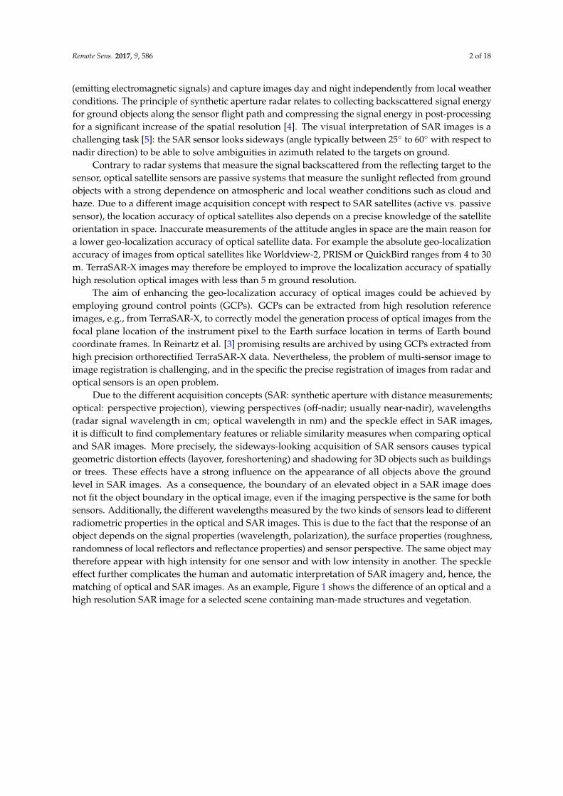
Due to the different acquisition concepts (SAR: synthetic aperture with distance measurements;optical: perspective projection), viewing perspectives (off-nadir; usually near-nadir), wavelengths(radar signal wavelength in cm; optical wavelength in nm) and the speckle effect in SAR images,it is difficult to find complementary features or reliable similarity measures when comparing opticaland SAR images. More precisely, the sideways-looking acquisition of SAR sensors causes typicalgeometric distortion effects (layover, foreshortening) and shadowing for 3D objects such as buildingsor trees. These effects have a strong influence on the appearance of all objects above the groundlevel in SAR images. As a consequence, the boundary of an elevated object in a SAR image doesnot fit the object boundary in the optical image, even if the imaging perspective is the same for bothsensors. Additionally, the different wavelengths measured by the two kinds of sensors lead to differentradiometric properties in the optical and SAR images. This is due to the fact that the response of anobject depends on the signal properties (wavelength, polarization), the surface properties (roughness,randomness of local reflectors and reflectance properties) and sensor perspective. The same object maytherefore appear with high intensity for one sensor and with low intensity in another. The speckleeffect further complicates the human and automatic interpretation of SAR imagery and, hence, thematching of optical and SAR images. As an example, Figure 1 shows the difference of an optical and ahigh resolution SAR image for a selected scene containing man-made structures and vegetation.

Remote Sens. 2017, 9, 586 3 of 18

Figure 1. Visual comparison of an optical (top) and SAR image (bottom) acquired over the same area.Both images have a ground sampling distance of 1.25 m.

1.2. Related Work

To improve the absolute geo-location accuracy of optical satellite images using SAR images asreference, the above-mentioned problems for SAR and optical image registration need to be dealtwith. Different research studies investigated the geo-localization accuracy improvement of opticalsatellite images based on SAR reference data, e.g., [3,6,7]. The related approaches rely on suitableimage registration techniques, which are tailored to the problem of optical and SAR images matching.

The aim of image registration is to estimate the optimal geometric transformation between twoimages. The most common multi-modal image registration approaches can be divided into twocategories. The first category comprises intensity-based approaches, where a transformation betweenthe images can be found by optimizing the corresponding similarity measure. Influenced by thefield of medical image processing, similarity measures like normalized cross-correlation [8], mutualinformation [9,10], cross-cumulative residual entropy [11] and the cluster reward algorithm [12] arefrequently used for SAR and optical image registration. A second approach is based on local frequencyinformation and a confidence-aided similarity measure [13]. Li et al. [14] and Ye et al. [15] introducedsimilarity measures based on the histogram of oriented gradients and the histogram of oriented phasecongruency, respectively. However, these approaches are often computationally expensive, sufferfrom the different radiometric properties of SAR and optical images and are sensitive to speckle in theSAR image.

Remote Sens. 2017, 9, 586 4 of 18

The second category comprises feature-based approaches, which rely on the detection andmatching of robust and accurate features from salient structures. Feature-based approaches are lesssensitive to radiometric differences of the images, but have problems in the detection of robust featuresfrom SAR images due to the impact of speckle. Early approaches are based on image features likelines [16], contours [17,18] or regions [19]. A combination of different features (points, straight lines,free-form curves or areal regions) is investigated in [20]. The approach shows good performance forthe registration of optical and SAR images, but the features from the SAR images have to be selectedmanually. As the matching between optical and SAR images usually fails using the scale-invariantfeature transform (SIFT), Fan [21] introduced a modified version of the algorithm. With the improvedSIFT, a fine registration for coarsely-registered images can be achieved, but the approach fails forimage pairs with large geometric distortions. To find matching points between area features, a levelset segmentation-based approach is introduced in [22]. This approach is limited to images that containsharp edges from runways, rivers or lakes. Sui et al. [23] and Xu et al. [22] propose iterative matchingprocedures to overcome the problem of misaligned images caused by imprecise extracted features.In [23], an iterative Voronoi spectral point matching between the line-intersection is proposed, whichdepends on the presence of salient straight line features in the images.

Other approaches try to overcome the drawbacks of intensity and feature-based approachesby combining them. A global coarse registration using mutual information on selected areas (nodense urban and heterogeneous areas) followed by a fine local registration based on linear features isproposed in [24]. As a drawback, the method highly depends on the coarse registration. If the coarseregistration fails, the fine registration will be unreliable.

Besides classical registration approaches, a variety of research studies indicate the high potentialof deep learning methods for different applications in remote sensing, such as classification ofhyperspectral data [25–27], enhancement of existing road maps [28,29], high-resolution SAR imageclassification [30] or pansharpening [31]. In the context of image matching, deep matching networkswere successfully trained for tasks such as stereo estimation [32,33], optical flow estimation [34,35],aerial image matching [36] or ground to aerial image matching [37]. In [38], a deep learning-basedmethod is proposed to detect and match multiscale keypoints with two separated networks. While thedetection network is trained on multiscale patches to identify regions including good keypoints, thedescription network is trained to match extracted keypoints from different images.

Most of the deep learning image matching methods are based on a Siamese networkarchitecture [39]. The basic idea of these methods is to train a neural network that is composedof two parts: the first part, a Siamese or pseudo-Siamese network, is trained to extract features fromimage patches, while the second part is trained to measure the similarity between these features.Several types of networks showed a high potential for automatic feature extraction from images, e.g.,stacked (denoising) autoencoders [40], restricted Boltzmann machines [41] or convolutional neuralnetworks (CNNs) [42]. From these networks, CNNs have been proven to be efficient for featureextraction and have seen successfully trained for image matching in [32,33,36–38,43–45]. A similaritymeasure, the L2 distance [45] or the dot product [32,33], is applied on a fully-connected network [43,44].The input of the network can be single-resolution image patches [36,43,45], multi-resolution patches[44] or patches that differ in size for the left and right branch of the Siamese network [32,44].

Summarizing, we are tackling the task of absolute geo-location accuracy improvement of opticalsatellite images by generating few, but very accurate and reliable matching points between SAR andoptical images with the help of a neural network. These points serve as input to improve the sensormodels for optical image acquisitions. The basis of the approach is a Siamese network, which is trainedto learn the spatial shift between optical and SAR image patches. Our network is trained on selectedpatches where the differences are mostly radiometric, as we try to avoid geometrical ones. The patchesfor training are semi-manually extracted from TerraSAR-X and PRISM image pairs that capture largerurban areas spread over Europe.

Remote Sens. 2017, 9, 586 5 of 18

2. Deep Learning for Image Matching

Our research objective is to compute a subset of very accurate and reliable matching pointsbetween SAR and optical images. Common optical and SAR image matching approaches are often notapplicable to a wide range of images acquired over different cities or at different times of the year. Thisproblem can be handled using a deep learning-based approach. Through training a suitable neuralnetwork on a large dataset containing images spread over Europe and acquired at different times ofthe year, the network will learn to handle radiometric changes of an object over time or at differentlocations in Europe. To avoid geometrical differences between the SAR and optical patches, we focusour training on patches containing flat surfaces such as streets or runways in rural areas. This is not astrong restriction of our approach as these features frequently appear in nearly every satellite image.

Inspired by the successful use of Siamese networks for the task of image matching, we adopt thesame architecture. A Siamese network consists of two parallel networks, which are connected at theiroutput node. If the parameters between the two networks are shared, the Siamese architecture providesthe advantage of consistent predictions. As both network branches compute the same function, it isensured that two similar images will be mapped to a similar location in the feature space. Our Siamesenetwork consists of two CNNs. In contrast to fully-connected or locally-connected networks, a CNNuses filters, which are deployed for the task of feature extraction. Using filters instead of full or localconnections reduces the amount of parameters within the network. Less parameters lead to a speedincrease in the training procedure and a reduction in the amount of required training data and, hence,reduce the risk of overfitting.

In comparison to common deep learning-based matching approaches, our input images areacquired from different sensors with different radiometric properties. Due to speckle in SAR images,the pre-processing of the images plays an important role during training and for the matching accuracyand precision of the results. Our dataset contains images with a spatial resolution of 2.5 m, andtherefore exhibit a lower level of detail in the images compared to the ones used in [32,43–45]. In orderto increase the probability of the availability of salient features in the input data, we use large inputpatches with at least a size of 201× 201 pixels. The mentioned problems require a careful selection ofthe network architecture to find the right trade-off between the number of parameters, the number oflayers and, more importantly, the receptive field size.

2.1. Dilation

In the context of CNNs, the receptive field refers to the part of the input patches, having animpact on the output of the last convolutional layer. To achieve the whole input patch having animpact on our network output, a receptive field size of 201× 201 pixels is desired. Standard waysto increase the receptive field size are strided convolutions or pooling (downsampling) layers insidethe neural network. Here, the word stride refers to the distance between two consecutive positionsof the convolution filters. This would introduce a loss of information as these approaches reduce theresolution of the image features. In contrast, dilated convolutions [46] systematically aggregateinformation through an exponential growth of the receptive without degradation in resolution.The dilated convolution ∗d at a given position p in the image F is defined as:

(F ∗d k)(p) =r

∑m=−r

F(p− d ·m)k(m), (1)

where k denotes the kernel/filter with size (2r + 1) × (2r + 1) and d denotes the dilation factor.Instead of looking at local (2r + 1)× (2r + 1) regions as in the case of standard convolutions, dilatedconvolutions look at [d · (2r + 1)]× [d · (2r + 1)] surrounding regions, which lead to an expansion of thereceptive field size. Beyond this, dilated convolutions have the same number of network parameterscompared to their convolution counterpart.

Remote Sens. 2017, 9, 586 6 of 18

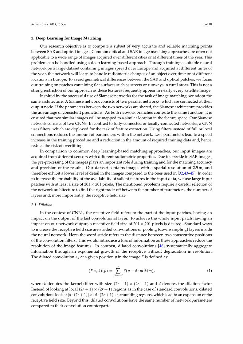
2.2. Network Architecture

Our matching network is composed of a feature extraction network (a Siamese network) followedby a layer to measure the similarity of the extracted features (the dot product layer). An overviewof the network architecture is depicted on the left side of Figure 2. The inputs of the left and rightbranches of the Siamese network are an optical (left) and a SAR (right) reference image, respectively.The weights of the two branches can be shared (Siamese architecture) or partly shared (pseudo-Siamesearchitecture).

optical image SAR image

CNN CNN

predicted shift

dot product

featu

reextraction

simila

ritymeasu

re

1

ConvBNReLU 5× 5 filter (32)

ConvBNReLU 5× 5 filter (32)

2-DilatedConvBNReLU 5× 5 filter (32)

4-DilatedConvBNReLU 5× 5 filter (32)

ConvBN 5× 5 filter (64)

16-DilatedConvBNReLU 5× 5 filter (64)

8-DilatedConvBNReLU 5× 5 filter (64)

ConvBNReLU 5× 5 filter (64)

16-DilatedConvBNReLU 5× 5 filter (64)

CNN

1

Figure 2. Network architecture (left) and a detailed overview of the convolutional layers (right).Abbreviations: convolutional neural network (CNN), convolution (Conv), batch normalization (BN)and rectified linear unit (ReLU).

Each layer of the network consists of a spatial convolution (Conv), a spatial batch normalization(BN) [47] and a rectified linear unit (ReLU). The purpose of the convolution layers is to extract spatialfeatures from the input data through trainable filters. The complexity of the features extracted bythe layers increases along with the depth. A normalization of the input data is often used as apre-processing step to increase the learning speed and the performance of the network. By passing theinput through the different layers of the network, the distribution of each single layer input changes.Therefore, BN is used in every layer of the network to ensure the consistency in the distribution ofthe layer inputs, as it provides a form of regularization and reduces the dependency of the networkperformance on the initialization of the weights. Non-linear activation functions like ReLUs are neededto introduce nonlinearities into the network (otherwise the network can only model linear functions).An Advantage of ReLUs compared to other activation function is a more efficient and faster training ofthe network.

We removed the ReLU from the last layer to preserve the information encoded in the negativevalues. In all layers convolutions with a filter size of 5× 5 pixels are employed. To overcome theproblem of our relatively large input patch size, we adopt dilation convolutions [46] for the layers threeto seven with a dilation factor d of 2, 4, 8 and 16 for the last two layers. This setup leads to the desiredreceptive field size of 201× 201 pixels. The number of filters used in layer one to four is 32 and for theothers is 64. The overall output is a predicted shift of the optical image within the SAR reference patch

Remote Sens. 2017, 9, 586 7 of 18

and is computed by taking the dot product of the output of the two branches. A detailed overview ofone branch of the Siamese network is the depicted on the right side of Figure 2.

2.3. SAR Image Pre-Processing

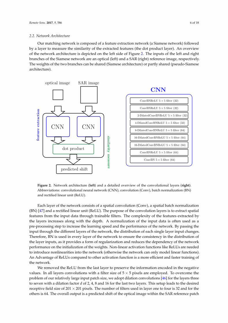
We use the probabilistic patch-based (PPB) filter proposed in [48] for the pre-processing of theSAR images. This filter is developed to suppress speckle in SAR images by adapting the non-localmean filter by Buades et al. [49] to SAR images. The idea of the non-local mean filter is to estimate thefiltered pixel value as the weighted average over all pixels in the image. The weights are measuringthe similarity between the pixel values of a patch ∆s centred around a pixel s and the pixel values ofa patch ∆t centred around a pixel t. The similarity between two patches is estimated through theirEuclidean distance. In [48], the noise distribution is modelled using the weighted maximum likelihoodestimator, in which the weights express the probability that two patches centred around the pixelss and t have the same noise distribution in a given image. The results of applying this filter and acomparison between SAR and optical patches are shown in Figure 3.

(a) (b) (c)

Figure 3. Visual comparison between optical (a), SAR (b) and despeckled SAR patches (c).

2.4. Matching Point Generation

We generate the matching points by training the network over a large dataset of optical andSAR image patch pairs, which have been manually co-registered. More precisely, the network istrained with smaller left image patches cropped from optical images and larger right images patchescropped from SAR images. Note that given a fixed size b× h of the left image patch L, the output ofthe network will depend on the size of the right image patch. The right image patch R has the size(b + s)× (h + s), where s defines the range over which we perform our search. The output of thenetwork is a two-dimensional scoring map with size (s + 1)× (s + 1) over the search space S withsize (b + s)× (h + s).

The scoring map si for the i-th input image pair contains a similarity score si,j for each location qi,jin the search space (j ∈ J = {1, . . . , |S|}, where |S| is the cardinality of S). The search space index Jis indexing the two-dimensional search space, where each position qi,j in S corresponds to a specifictwo-dimensional shift of the left optical patch with respect to the larger SAR patch.

To get the similarity scores for every image pair, we first compute the feature vector fi for thei-th optical training patch and the feature matrix hi for the corresponding i-th SAR patch. The featurevector fi is the output of the left network branches and has a dimension of 64 (as the last convolutionlayer has 64 filters). The feature matrix hi is the output of the right network branch with a dimension

Remote Sens. 2017, 9, 586 8 of 18

of |S| × 64 and is composed of the feature vectors hi,j for each location in the search space. We thencompute the similarity of the features vectors fi and hi,j for every position qi,j ∈ S.

To measure the similarity between the two vectors, we use the dot product and obtain thesimilarity scores si,j = fi · hi,j for all j ∈ J. A high value of si,j indicates a high similarity between thetwo vectors fi and hi,j at location qi,j (which is related to a two-dimensional pixel shift). In other words,a high similarity score si,j indicates a high similarity between the i-th optical patch and the i-th SARpatch at location qi,j in our search space. To get a normalized score over all locations within the searchspace, we apply the soft-max function at each location qi,j ∈ S:

s̃i,j =exp(si,j)

∑j∈J

exp(si,j). (2)

This function is commonly used for multi-class classification problems to compute the probabilitythat a certain training patch belongs to a certain class. In our case, the normalized score s̃i,j can beinterpreted as a probability for the specific shift, which corresponds to location qi,j with index j. Thus,the output of our network (the normalized score map) can be seen as a probability distribution with aprobability for every location (shift) of the optical patch within the SAR image patch.

By treating the problem as a multi-class classification problem, where the different classesrepresent the possible shifts of an optical patch with respect to a larger SAR patch, we train ournetwork by minimizing the cross entropy loss:

minw ∑

i∈I,j∈Jpgt(qi,j) log pi(qi,j, w) (3)

with respect to the weights w, which parametrize our network. Here, pi(qi,j, w) is the predicted scorefor sample i at location qi,j in our search space, and pgt is the ground truth target distribution. Insteadof a delta function with non-zero probability mass only at the correct location qi,j = qgt

i , we are using asoft ground truth distribution, which is centred around the ground truth location. Therefore, we setpgt to be the discrete approximation of the Gaussian function (with σ = 1) in an area around qgt

i :

pgt(qi,j) =

12π · e−

∥∥∥qi,j−qgti

∥∥∥2

22 if

∥∥∥qi,j − qgti

∥∥∥2< 3

0 otherwise, (4)

where ‖·‖2 denotes the L2 (Euclidean) distance. We use stochastic gradient descent with Adam [50] tominimize our loss function (3) and, hence, to train our network to learn the matching between opticaland SAR patches.

After training, we keep the learned parameters w fixed and decompose the network into twoparts: the feature extractor (CNN) and the similarity measure (dot product layer). As the featureextractor is convolutional, we can apply the CNN on images with an arbitrary size. Thus, during thetest time, we first give an optical patch as input to the CNN and compute the feature vector f . Thenwe consider a larger SAR patch which covers the desired search space, and compute the feature matrixh. Afterwards, we use the dot product layer to compute the normalized score map from f and h (in thesame way as for the training step). Applying this strategy, we can compute a matching score betweenoptical patches with arbitrary size and SAR images over an arbitrary search space. We obtain thematching points (predicted shifts) by picking for every input image pair the points with the highestvalue (highest similarity between optical and SAR patch) within the corresponding search space.

Remote Sens. 2017, 9, 586 9 of 18

2.5. Geo-Localization Accuracy Improvement

The inaccuracy of the absolute geo-localization of the optical satellite data in the geo-referencingprocess arises mainly from inaccurate measurements of the satellite attitude and thermally-affectedmounting angles between the optical sensor and the attitude measurement unit. This insufficientpointing knowledge leads to local geometric distortions of orthorectified images caused by the heightvariations of the Earth’s surface. To achieve higher geometric accuracy of the optical data, groundcontrol information is needed to adjust the parameters of the physical sensor model. We are followingthe approach described in [51] to estimate the unknown parameters of the sensor model from GCPs byiterative least squares adjustment. In order to get a reliable set of GCP, different levels of point filteringand blunder detection are included in the processing chain. In contrast to [51], where the GCPs aregenerated from an optical image, we are using the matching points generated by our network.

3. Experimental Evaluation and Discussion

To perform our experiments, we generated a dataset out of 46 orthorectified optical (PRISM) andradar (TerraSAR-X acquired in stripmap mode) satellite image pairs acquired over 13 city areas inEurope. The images include suburban, industrial and rural areas with a total coverage of around20, 000 km2. The spatial resolution of the optical images is 2.5 m, and the pixel spacing of the SARimages is 1.25 m. To have a consistent pixel spacing within the image pairs, we downsampled the SARimages to 2.5 m using bilinear interpolation.

As the ground truth, we are using optical images which were aligned to the corresponding SARimages in the Urban Atlas project [52]. The alignment between the images was achieved by a manualselection of several hundred matching points for every image pair. These matching points are usedto improve the sensor model related to the optical images. By using the improved sensor models toorthorectify the optical images, the global alignment error could be reduced from up to 23 m to around3 m in this project.

To minimize the impact of the different acquisition modes of PRISM and TerraSAR-X, we focuson flat surfaces where only the radiometry between the SAR and optical images is different. Therefore,patches are favored that contain parts of streets or runways in rural areas. The patches are pre-selectedusing the CORINE land cover [53] from the year 2012 to exclude patches, e.g., containing streetsegments in city areas. The CORINE layer includes 44 land cover classes and has a pixel size of100 m. For the pre-selection, the following classes are chosen: airports, non-irrigated arable land,permanently-irrigated land, annual crops associated with permanent crops and complex cultivationpatterns, land principally occupied by agriculture, with significant areas of natural vegetation. Notethat there are several current global land cover maps available, which enable a similar pre-selectionfor images outside Europe. The pre-selection was refined manually to ensure that the patches containstreets/runways segments that are visible in the optical and the SAR patches and to avoid patchescontaining street segments through smaller villages or areas covered by clouds in the optical images.

3.1. Dataset Generation

The training, validation and test datasets are generated by randomly splitting the 46 images into 36images for training, 4 for validation and 6 for testing. As a form of data augmentation, we use bilinearinterpolation to downsample the optical and SAR images, which are used for training, to a pixel spacingof 3.75 m. This leads to a training set with a total number of 92 images for each sensor, where half ofthe images have a resolution of 2.5 m and the other half of 3.75 m. Data augmentation is commonlyused to generate a larger training dataset and, hence, to prevent the network from overfitting.

The training, validation and test patches are cropped from the images of the corresponding sets.The optical patches have a size of 201× 201 pixels, and the SAR patches have a size of 221× 221 pixels.The final dataset contains 135,000 pairs of training patches, 5000 pairs of validation patches and14,400 pairs of test patches, and the total number of search locations is 441. Note that the alignment

Remote Sens. 2017, 9, 586 10 of 18

error between the SAR and the optical image is expected to be not larger than 32 m. Therefore, a21× 21 pixel search space with a pixel spacing of 2.5 m in the validation and test case is assumed to belarge enough.

3.2. Training Parameters

Our network is trained with 100 rounds, where each round takes 200 iterations over a singlebatch. The initial learning rate is set to 0.01, and we reduce it by a factor of five at iterations 60 and 80.We train the network in parallel on two Titan X GPUs using a batch size of 100. The weights of thenetwork are initialized with the scheme described in [54], which particularly considers the rectifiernonlinearities. The whole training process takes around 30 h.

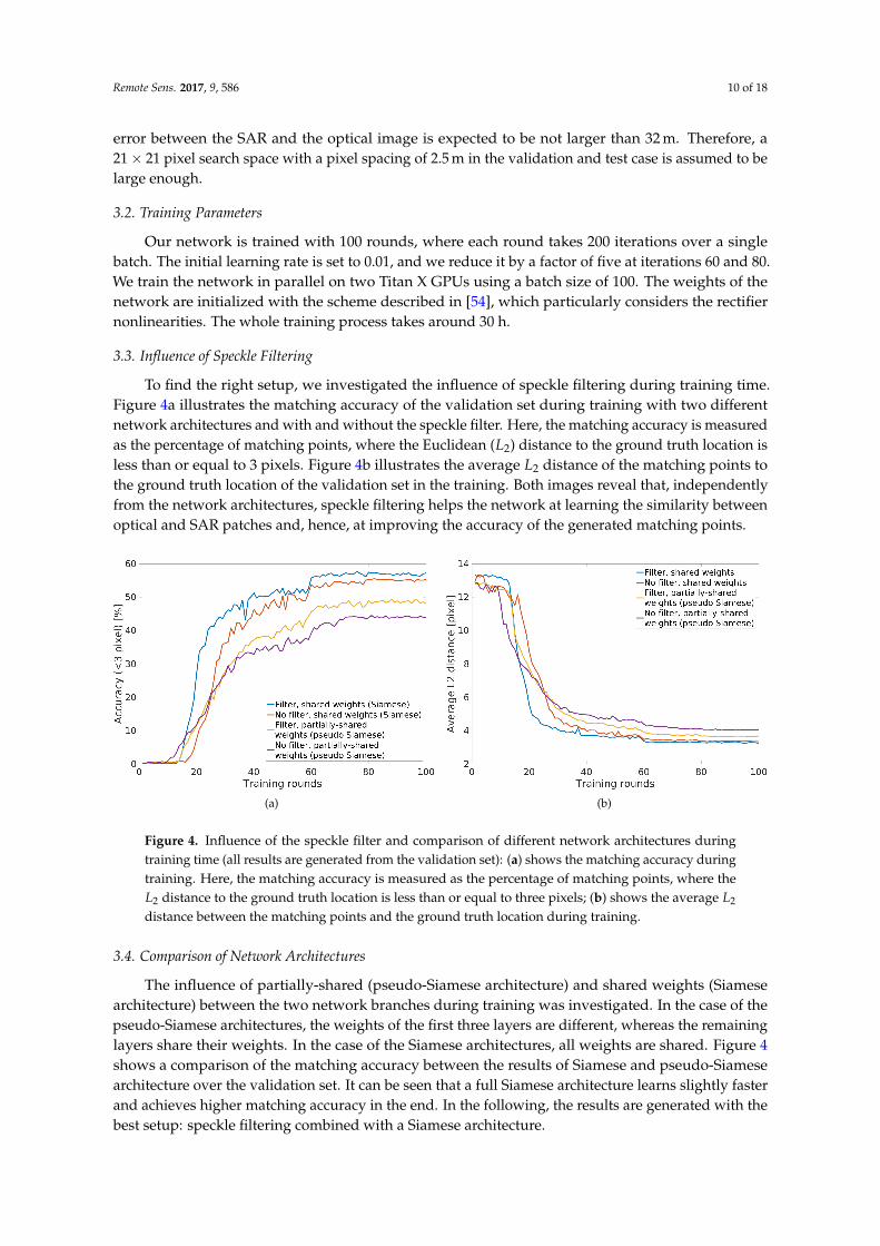
3.3. Influence of Speckle Filtering

To find the right setup, we investigated the influence of speckle filtering during training time.Figure 4a illustrates the matching accuracy of the validation set during training with two differentnetwork architectures and with and without the speckle filter. Here, the matching accuracy is measuredas the percentage of matching points, where the Euclidean (L2) distance to the ground truth location isless than or equal to 3 pixels. Figure 4b illustrates the average L2 distance of the matching points tothe ground truth location of the validation set in the training. Both images reveal that, independentlyfrom the network architectures, speckle filtering helps the network at learning the similarity betweenoptical and SAR patches and, hence, at improving the accuracy of the generated matching points.

(a) (b)

Figure 4. Influence of the speckle filter and comparison of different network architectures duringtraining time (all results are generated from the validation set): (a) shows the matching accuracy duringtraining. Here, the matching accuracy is measured as the percentage of matching points, where theL2 distance to the ground truth location is less than or equal to three pixels; (b) shows the average L2

distance between the matching points and the ground truth location during training.

3.4. Comparison of Network Architectures

The influence of partially-shared (pseudo-Siamese architecture) and shared weights (Siamesearchitecture) between the two network branches during training was investigated. In the case of thepseudo-Siamese architectures, the weights of the first three layers are different, whereas the remaininglayers share their weights. In the case of the Siamese architectures, all weights are shared. Figure 4shows a comparison of the matching accuracy between the results of Siamese and pseudo-Siamesearchitecture over the validation set. It can be seen that a full Siamese architecture learns slightly fasterand achieves higher matching accuracy in the end. In the following, the results are generated with thebest setup: speckle filtering combined with a Siamese architecture.

Remote Sens. 2017, 9, 586 11 of 18

3.5. Comparison to Baseline Methods

For a better evaluation of our results, we compare our method with three available baselinemethods: the similarity measure normalized cross-correlation (NCC) [55], the similarity measuremutual information (MI) [56], and a MI-based method (CAMRI) which is tailored to the problem ofoptical and SAR matching [10]. To ensure a fair comparison, we applied the pre-processing with thespeckle filter [48] to all baseline methods, except for CAMRI [10]. Here, a slightly different speckle filteris implemented internally. Table 1 shows the comparison of our method with the baseline methods.The expression “Ours (score)” denotes our method, where we used a threshold to detect outliers andto generate more precise and reliable matching points (detailed explanation in the next section). “Ours(scores)” achieves higher matching accuracy and precision than NCC, MI and CAMRI [10]. Moreprecisely, the average value over the L2 distances between the matching points and the ground truthlocations is the smallest (measured in pixel units) for our method. Furthermore, the comparison of thematching precisions reveals that our matching points, with a standard deviation σ of 1.14 pixels, arethe most reliable ones. The running time of our method during test time is 3.3 m for all 14,000 testpatches on a single GPU. The baseline methods are running on CPU, which makes a fair comparisondifficult, but CAMRI [10] requires around three days to compute the matching points for the test set.

Table 1. Comparison of the matching accuracy and precision of our method with accuracies ofnormalized cross-correlation (NCC), mutual information (MI) and CAMRI [10] over the test set. Thematching accuracy is measured as the percentage of matching points, having a L2 distance to theground truth location smaller than a specific number of pixels and as the average over the L2 distancesbetween the predicted matching points and the ground truth locations (measured in pixel units). Thematching precision is represented by the standard deviation σ (measured in pixel units).

Methods Matching Accuracy Matching Precision<2 pixels <3 pixels <4 pixels avg L2 (pixel) σ (pixel)

NCC 2.94% 7.92% 13.01% 9.92 4.04MI 18.18% 38.60% 51.99% 4.89 3.64

CAMRI [10] 33.55% 57.06% 79.93% 2.80 2.86

Ours 25.40% 49.60% 64.28% 3.91 3.17Ours (score) 49.70% 82.80% 94.70% 1.91 1.14

3.6. Outlier Removal

So far, we used the normalized score (after applying the soft-max) and we selected the locationswith the highest value (highest probability) within each search area as the predicted matching pointafter a two-dimensional shift. Another possibility is to use the raw score (before soft-max) as anindicator of the confidence of the prediction. Utilizing this information, we can aggregate thepredictions from the network to detect outliers and achieve higher matching performances. Therefore,we investigated the influence of the raw score as a threshold as shown in Figure 5, which enablesthe detection of correct predicted matching points. A higher threshold on the raw score leads to abetter accuracy in terms of correct prediction, as well as a smaller L2 distance between the predictedmatching points and the ground truth locations. Note that the rough shape at the right side of thecurves in Figure 5b,c is the result of an outlier. Here, an outlier has a strong influence, since thesenumbers are computed from less than 20 test patches.

By using only the first 1000 matches with the highest raw score, the average over the L2 distancesbetween the matching points and the ground truth location can be reduced from 3.91 pixels (usingall matches) to 1.91 pixels, and the standard deviation (matching precision) from 3.37 to 1.14 pixels(see Table 1). Note that a higher threshold results in a smaller number of valid matching points, whichare more reliable (in terms of the L2 distance). For a later application, a threshold does not have to

Remote Sens. 2017, 9, 586 12 of 18

be specified. Depending on the number of matching points x needed for an image pair, the best xmatching points can be chosen, based on the raw score.

(a) (b)

(c) (d)

Figure 5. Illustration of influence of the raw score as a threshold: (a) the relation between the predictedscore and the number of patches; (b) relation between the number of patches and the matchingaccuracy; (c) relation between the predicted score and the matching accuracy; and (d) relation betweenthe predicted score and the average distance (L2) between the predicted matching points and theground truth location. The matching accuracy in Figure 5b is measured as the percentage of matchingpoints, where the L2 distance to the ground truth location is less than three pixels and in Figure 5c lessthan 2, 3 and 4 pixels.

3.7. Qualitative Results

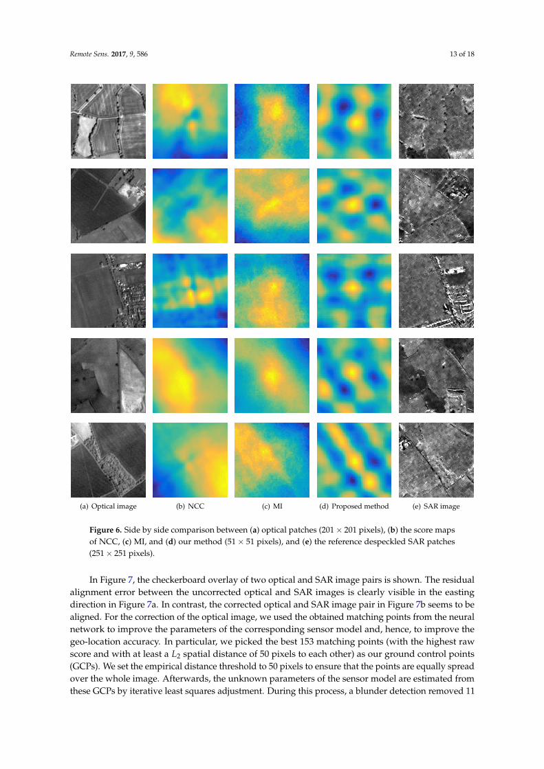
In Figure 6, we show a side by side comparison of the score maps of our approach with twobaseline methods of sample image patches. Note that CAMRI [10] does not provide a score map asoutput. Therefore, we perform our search over a 51× 51 pixels search space, where the used patcheshave a resolution of 2.5 m. The images in the first column are optical image patches and the imagesin the last column the despeckled SAR image patches. To generate the images in column 2 to 4 weperform the matching between the corresponding image pairs using NCC, MI and our method. Yellowindicates a higher score, and blue indicates a lower score. The ground truth location is in the center ofeach patch. Our approach performs consistently better than the corresponding baseline methods. Moreprecisely, the score maps generated with our approach show one high peak at the correct position,except for the last example. Here, two peaks are visible along a line, which corresponds to a street inthe SAR patch. In contrast, both baseline methods show a relatively large area with a constantly highscore at the wrong positions for most examples.

Remote Sens. 2017, 9, 586 13 of 18

(a) Optical image (b) NCC (c) MI (d) Proposed method (e) SAR image

Figure 6. Side by side comparison between (a) optical patches (201× 201 pixels), (b) the score mapsof NCC, (c) MI, and (d) our method (51× 51 pixels), and (e) the reference despeckled SAR patches(251× 251 pixels).

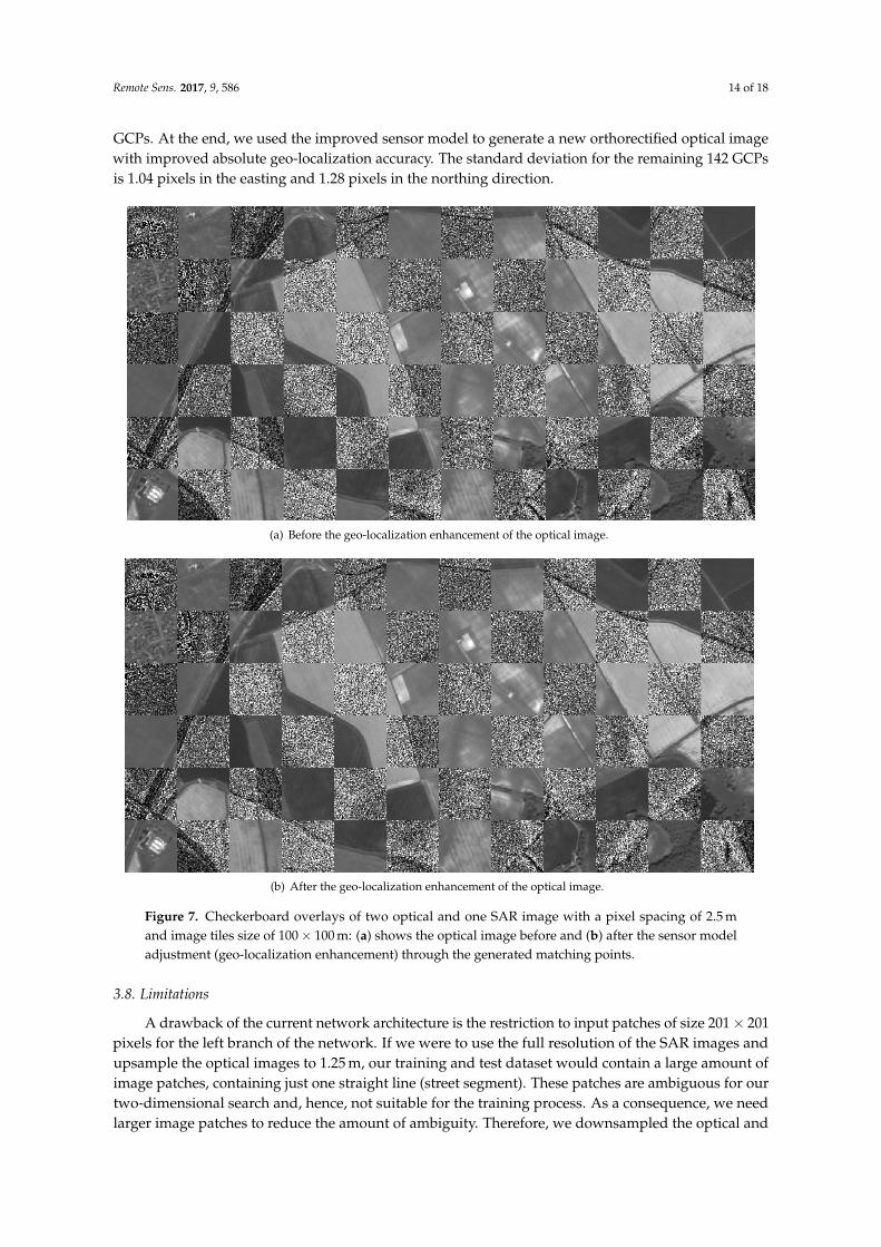
In Figure 7, the checkerboard overlay of two optical and SAR image pairs is shown. The residualalignment error between the uncorrected optical and SAR images is clearly visible in the eastingdirection in Figure 7a. In contrast, the corrected optical and SAR image pair in Figure 7b seems to bealigned. For the correction of the optical image, we used the obtained matching points from the neuralnetwork to improve the parameters of the corresponding sensor model and, hence, to improve thegeo-location accuracy. In particular, we picked the best 153 matching points (with the highest rawscore and with at least a L2 spatial distance of 50 pixels to each other) as our ground control points(GCPs). We set the empirical distance threshold to 50 pixels to ensure that the points are equally spreadover the whole image. Afterwards, the unknown parameters of the sensor model are estimated fromthese GCPs by iterative least squares adjustment. During this process, a blunder detection removed 11

Remote Sens. 2017, 9, 586 14 of 18

GCPs. At the end, we used the improved sensor model to generate a new orthorectified optical imagewith improved absolute geo-localization accuracy. The standard deviation for the remaining 142 GCPsis 1.04 pixels in the easting and 1.28 pixels in the northing direction.

(a) Before the geo-localization enhancement of the optical image.

(b) After the geo-localization enhancement of the optical image.

Figure 7. Checkerboard overlays of two optical and one SAR image with a pixel spacing of 2.5 mand image tiles size of 100× 100 m: (a) shows the optical image before and (b) after the sensor modeladjustment (geo-localization enhancement) through the generated matching points.

3.8. Limitations

A drawback of the current network architecture is the restriction to input patches of size 201× 201pixels for the left branch of the network. If we were to use the full resolution of the SAR images andupsample the optical images to 1.25 m, our training and test dataset would contain a large amount ofimage patches, containing just one straight line (street segment). These patches are ambiguous for ourtwo-dimensional search and, hence, not suitable for the training process. As a consequence, we needlarger image patches to reduce the amount of ambiguity. Therefore, we downsampled the optical and

Remote Sens. 2017, 9, 586 15 of 18

SAR images. Due to the memory limits of our available GPUs, it was not possible to increase the inputpatch size and simultaneously keep a proper batch size. A possible solution could be the investigationof a new network architecture, which enables the use of larger input patches. An alternative solutioncould be a better selection process of the patches, e.g., only patches containing street crossings.

The processing chain for the generation of our dataset and the relatively small amount of trainingdata represent the main current weaknesses. The selection of the image patches for the dataset wasmainly done manually and is limited to one SAR and optical satellite sensor (PRISM and TerraSAR-X).Through the usage of OpenStreetMap and/or a road segmentation network, the generation of thedataset could be done automatically, and our datasets could be quickly extended with new imagepatches. A larger dataset would help to deal with the problem of overfitting during training, andfurther improve the network performance.

Additionally, the success of our approach depends on the existence of salient features in theimage scene. To generate reliable matching points, these features have to exhibit the same geometricproperties in the optical and SAR image, e.g., street-crossings. Therefore, the proposed method is nottrained to work on images without such features, e.g., images covering only woodlands, mountainousareas or deserts.

3.9. Strengths

The results prove the potential of our method for the task of geo-localization improvement ofoptical images through SAR reference data. By interpreting the raw network output as the confidencefor predicted matching points (predicted shifts) between optical and SAR patches, we are able togenerate matching points with high matching accuracy and precision. Furthermore, the high qualityof the matching points does not increase the computation time. After training, we can compute newmatching points between arbitrary optical and SAR image pairs within seconds. In contrast, a MI-basedapproach like CAMRI [10] needs several hours or days to compute the matching points between thesame image patches, yielding in less accurate and precise results.

In contrast to other deep learning-based matching approaches, our network is able to matchmulti-sensor images with different radiometric properties. Our neural network is extendible to imagesfrom other optical or radar sensors with little effort, and it is applicable to multi-resolution images.In contrast to other feature-based matching approaches, our method is based on reliable (in termsof equal geometric properties in the optical and SAR image patches) features, e.g., streets and streetcrossings, which frequently appear in many satellite images. Furthermore, through the variety inour training image pairs, our method is applicable to a wide range of images acquired over differentcountries or at different times of the year.

4. Conclusions

In this paper, the applicability of a deep learning-based approach for the geo-localization accuracyimprovement of optical satellite images through SAR reference data is confirmed for the first time.For this purpose, a neural network has been trained to learn the spatial shift between optical andSAR image patches. The network is composed of a feature extraction part (Siamese network) anda similarity measure part (dot product layer). The network was trained on 134,000 and tested on14,000 pairs of patches cropped from optical (PRISM) and SAR (TerraSAR-X) satellite image pairs over13 city areas spread over Europe.

The effectiveness of our approach for the generation of accurate and reliable matching pointsbetween optical and SAR images patches has been demonstrated. Our method outperformsstate-of-the-art matching approaches, like CAMRI [10]. Particular, matching points can be achievedwith an average L2 distance to the ground truth locations of 1.91 pixels and a precision (standarddeviation) of 1.14 pixels. Furthermore, by utilizing the resulting improved sensor model for thegeo-referencing and orthorectification processes, we achieve an enhancement of the geo-localizationaccuracy of the optical images.

Remote Sens. 2017, 9, 586 16 of 18

In the future, we will further enhance the accuracy and precision of the resulting matching pointsby using interpolation or polynomial curve fitting techniques to generate sub-pixel two-dimensionalshifts. Additionally, we are planning to investigate the influence of alternative network architectures,similarity measures and loss functions on the accuracy and precision of the matching points, as well asthe applicability of an automatic processing chain for the dataset generation using OpenStreetMapand a road detection network.

Acknowledgments: We gratefully thank Mathias Schneider for helping with the generation of our dataset, GeraldBaier for helping with the pre-processing of the TerraSAR-X images and Peter Schwind for his valuable suggestionsand support during the whole process.

Author Contributions: Nina Merkle, Wenjie Luo, Stefan Auer, Rupert Müller and Raquel Urtasun conceived anddesigned the experiments. Nina Merkle and Wenjie Luo wrote the source code. Nina Merkle generated the dataset,performed the experiments and wrote the paper. Wenjie Luo, Stefan Auer, Rupert Müller and Raquel Urtasunprovided detailed advice during the writing process. Rupert Müller and Raquel Urtasun supervised the wholeprocess and improved the manuscript.

Conflicts of Interest: The authors declare no conflict of interest.

References

1. Werninghaus, R.; Buckreuss, S. The TerraSAR-X Mission and System Design. IEEE Trans. Geosci. Remote Sens.2010, Vol. 48, pp. 606–614.

2. Eineder, M.; Minet, C.; Steigenberger, P.; Cong, X.; Fritz, T. Imaging Geodesy- Toward Centimeter-LevelRanging Accuracy with TerraSAR-X. IEEE Trans. Geosci. Remote Sens. 2011, Vol. 49, pp. 661–671.

3. Reinartz, P.; Müller, R.; Schwind, P.; Suri, S.; Bamler, R. Orthorectification of VHR Optical Satellite DataExploiting the Geometric Accuracy of TerraSAR-X Data. ISPRS J. Photogramm. Remote Sens. 2011, Vol. 66, pp.124–132.

4. Cumming, I.; Wong, F. Digital Processing of Synthetic Aperture Radar Data: Algorithms and Implementation;Number Bd. 1 in Artech House Remote Sensing Library; Artech House Inc., Boston, London, 2005.

5. Auer, S.; Gernhardt, S. Linear Signatures in Urban SAR Images—Partly Misinterpreted? IEEE Geosci. RemoteSens. Lett. 2014, Vol. 11, pp. 1762–1766.

6. Merkle, N.; Müller, R.; Reinartz, P. Registration of Optical and SAR Satellite Images based on GeometricFeature Templates. ISPRS - International Archives of the Photogrammetry, Remote Sensing and Spatial InformationSciences, Vol. XL-1/W5, 2015, pp. 447–452.

7. Perko, R.; Raggam, H.; Gutjahr, K.; Schardt, M. Using Worldwide Available TerraSAR-X Data to Calibratethe Geo-location Accuracy of Optical Sensors. In Proceedings of the 2011 IEEE International Geoscience andRemote Sensing Symposium, IGARSS, Vancouver, BC, Canada, 24–29 July 2011; pp. 2551–2554.

8. Shi, W.; Su, F.; Wang, R.; Fan, J. A Visual Circle Based Image Registration Algorithm for Optical and SARImagery. In Proceedings of the 2012 IEEE International Geoscience and Remote Sensing Symposium, Munich,Germany, 22–27 July 2012; pp. 2109–2112.

9. Siddique, M.A.; Sarfraz, M.S.; Bornemann, D.; Hellwich, O. Automatic Registration of SAR and OpticalImages Based on Mutual Information Assisted Monte Carlo. In Proceedings of the 2012 IEEE InternationalGeoscience and Remote Sensing Symposium, Munich, Germany, 22–27 July 2012; pp. 1813–1816.

10. Suri, S.; Reinartz, P. Mutual-Information-Based Registration of TerraSAR-X and Ikonos Imagery in UrbanAreas. IEEE Trans. Geosci. Remote Sens. 2010, Vol. 48, pp. 939–949.

11. Hasan, M.; Pickering, M.R.; Jia, X. Robust Automatic Registration of Multimodal Satellite Images UsingCCRE with Partial Volume Interpolation. IEEE Trans. Geosci. Remote Sens. 2012, Vol. 50, pp. 4050–4061.

12. Inglada, J.; Giros, A. On the Possibility of Automatic Multisensor Image Registration. IEEE Trans. Geosci.Remote Sens. 2004, Vol. 42, pp. 2104–2120.

13. Liu, X.; Lei, Z.; Yu, Q.; Zhang, X.; Shang, Y.; Hou, W. Multi-Modal Image Matching Based on Local FrequencyInformation. EURASIP J. Adv. Signal Process. 2013, pp. 1–11.

14. Li, Q.; Qu, G.; Li, Z. Matching Between SAR Images and Optical Images Based on HOG Descriptor.In Proceedings of the Radar Conference 2013, IET International, Xi’an, China, 14–16 April 2013; pp. 1–4.

Remote Sens. 2017, 9, 586 17 of 18

15. Ye, Y.; Shen, L. HOPC: A Novel Similarity Metric Based on Geometric Structural Properties for Multi-modalRemote Sensing Image Matching. ISPRS Ann. Photogramm. Remote Sens. Spat. Inf. Sci. 2016, Vol. III-1, pp.9–16.

16. Hong, T.D.; Schowengerdt, R.A. A Robust Technique for Precise Registration of Radar and Optical SatelliteImages. Photogramm. Eng. Remote Sens. 2005, Vol. 71, pp. 585–593.

17. Li, H.; Manjunath, B.S.; Mitra, S.K. A Contour-Based Approach to Multisensor Image Registration.IEEE Trans. Image Process. 1995, Vol. 4, pp. 320–334.

18. Pan, C.; Zhang, Z.; Yan, H.; Wu, G.; Ma, S. Multisource Data Registration Based on NURBS Description ofContours. Int. J. Remote Sens. 2008, Vol. 29, pp. 569–591.

19. Dare, P.; Dowmanb, I. An Improved Model for Automatic Feature-Based Registration of SAR and SPOTImages. ISPRS J. Photogramm. Remote Sens. 2001, Vol. 56, pp. 13–28.

20. Long, T.; Jiaoa, W.; Hea, G.; Zhanga, Z.; Chenga, B.; Wanga, W. A Generic Framework for Image RectificationUsing Multiple Types of Feature. ISPRS J. Photogramm. Remote Sens. 2015, Vol. 102, pp. 161–171.

21. Fan, B.; Huo, C.; Pan, C.; Kong, Q. Registration of Optical and SAR Satellite Images by Exploring the SpatialRelationship of the Improved SIFT. IEEE Geosci. Remote Sens. Lett. 2013, Vol. 10, pp. 657–661.

22. Xu, C.; Sui, H.; Li, H.; Liu, J. An Automatic Optical and SAR Image Registration Method with Iterative LevelSet Segmentation and SIFT. Int. J. Remote Sens. 2015, Vol. 36, pp. 3997–4017.

23. Sui, H.; Xu, C.; Liu, J.; Hua, F. Automatic Optical-to-SAR Image Registration by Iterative Line Extraction andVoronoi Integrated Spectral Point Matching. IEEE Trans. Geosci. Remote Sens. 2015, Vol. 53, pp. 6058–6072.

24. Han, Y.; Byun, Y. Automatic and Accurate Registration of VHR Optical and SAR Images Using a QuadtreeStructure. Int. J. Remote Sens. 2015, Vol. 36, pp. 2277–2295.

25. Chen, Y.; Lin, Z.; Zhao, X.; Wang, G.; Gu, Y. Deep Learning-Based Classification of Hyperspectral Data.Sel. Top. Appl. Earth Obs. Remote Sens. IEEE J. 2014, Vol. 7, pp. 2094–2107.

26. Liang, H.; Li, Q. Hyperspectral Imagery Classification Using Sparse Representations of ConvolutionalNeural Network Features. Remote Sens. 2016, Vol. 8(2), 99.

27. Wang, Q.; Lin, J.; Yuan, Y. Salient Band Selection for Hyperspectral Image Classification via ManifoldRanking. IEEE Trans. Neural Netw. Learn. Syst. 2016, Vol. 27, pp. 1279–1289.

28. Mnih, V.; Hinton, G.E. Learning to Detect Roads in High-Resolution Aerial Images. In ComputerVision—ECCV 2010, Proceedings of the 11th European Conference on Computer Vision, Heraklion, Crete, Greece,5–11 September 2010; Springer: Berlin/Heidelberg, Germany, 2010; Part VI, pp. 210–223.

29. Matthyus, G.; Wang, S.; Fidler, S.; Urtasun, R. HD Maps: Fine-grained Road Segmentation by ParsingGround and Aerial Images. In Proceedings of the IEEE International Conference on Computer Vision (ICCV), LasVegas, NV, USA, 27–30 June 2016; pp. 3611–3619.

30. Geng, J.; Fan, J.; Wang, H.; Ma, X.; Li, B.; Chen, F. High-Resolution SAR Image Classification via DeepConvolutional Autoencoders. Geosci. Remote Sens. Lett. IEEE 2015, Vol. 12, pp. 2351–2355.

31. Masi, G.; Cozzolino, D.; Verdoliva, L.; Scarpa, G. Pansharpening by Convolutional Neural Networks.Remote Sens. 2016, Vol. 8, 594.

32. Luo, W.; Schwing, A.G.; Urtasun, R. Efficient Deep Learning for Stereo Matching. In Proceedings of the IEEEConference on Computer Vision and Pattern Recognition (CVPR), Las Vegas, NV, USA, 27–30 June 2016.

33. Zbontar, J.; LeCun, Y. Stereo Matching by Training a Convolutional Neural Network to Compare ImagePatches. J. Mach. Learn. Res. 2016, Vol. 17, pp. 1–32.

34. Bai, M.; Luo, W.; Kundu, K.; Urtasun, R. Exploiting Semantic Information and Deep Matching for OpticalFlow. In Proceedings of the European Conference on Computer Vision (ECCV), Amsterdam, The Netherlands,8-16 October 2016.

35. Weinzaepfel, P.; Revaud, J.; Harchaoui, Z.; Schmid, C. DeepFlow: Large Displacement OpticalFlow withDeep Matching. In Proceedings of the IEEE Intenational Conference on Computer Vision (ICCV), Sydney, Australia,1–8 December 2013.

36. Altwaijry, H.; Trulls, E.; Hays, J.; Fua, P.; Belongie, S. Learning to Match Aerial Images with Deep AttentiveArchitectures. In Proceedings of the IEEE Conference on Computer Vision and Pattern Recognition (CVPR), LasVegas, NV, USA, 27–30 June 2016.

37. Lin, T.Y.; Cui, Y.; Belongie, S.; Hays, J. Learning Deep Representations for Ground-to-Aerial Geolocalization.In Proceedings of the IEEE Conference on Computer Vision and Pattern Recognition (CVPR), Boston, MA, USA,7-12 June 2015.

Remote Sens. 2017, 9, 586 18 of 18

38. Altwaijry, H.; Veit, A.; Belongie, S. Learning to Detect and Match Keypoints with Deep Architectures.In Proceedings of the British Machine Vision Conference (BMVC), York, UK, 19-22 September 2016.

39. Bromley, J.; Guyon, I.; LeCun, Y.; Säckinger, E.; Shah, R. Signature Verification using a “Siamese” Time DelayNeural Network. In Proceedings of the Conference on Neural Information Processing Systems (NIPS), Denver,Colorado, USA, 28 Nov.-1 December 1994.

40. Vincent, P.; Larochelle, H.; Lajoie, I.; Bengio, Y.; Manzagol, P.A. Stacked Denoising Autoencoders: LearningUseful Representations in a Deep Network with a Local Denoising Criterion. J. Mach. Learn. Res. 2010, Vol.11, pp. 3371–3408.

41. Fischer, A.; Igel, C. An Introduction to Restricted Boltzmann Machines. In Progress in Pattern Recognition,Image Analysis, Computer Vision, and Applications, Proceedings of the 17th Iberoamerican Congress, CIARP 2012,Buenos Aires, Argentina, 3–6 September 2012; Springer: Berlin/Heidelberg, Germany, 2012; pp. 14–36.

42. Krizhevsky, A.; Sutskever, I.; Hinton, G.E. ImageNet Classification with Deep Convolutional NeuralNetworks. In Proceedings of the Advances in Neural Information Processing Systems (NIPS), Lake Tahoe, USA,3-8 December 2012.

43. Han, X.; Leung, T.; Jia, Y.; Sukthankar, R.; Berg, A.C. MatchNet: Unifying Feature and Metric Learningfor Patch-Based Matching. In Proceedings of the IEEE Conference on Computer Vision and Pattern Recognition(CVPR), Boston, MA, USA, 7–12 June 2015.

44. Zagoruyko, S.; Komodakis, N. Learning to Compare Image Patches via Convolutional Neural Networks.In Proceedings of the IEEE Conference on Computer Vision and Pattern Recognition (CVPR), Boston, MA, USA,7–12 June 2015.

45. Simo-Serra, E.; Trulls, E.; Ferraz, L.; Kokkinos, I.; Fua, P.; Moreno-Noguer, F. Discriminative Learning ofDeep Convolutional Feature Point Descriptors. In Proceedings of the International Conference on ComputerVision (ICCV), Santiago, Chile, 11-18 December 2015.

46. Yu, F.; Koltun, V. Multi-Scale Context Aggregation by Dilated Convolutions. In International Conference onLearning Representations (ICCV), San Juan, Puerto Rico, 2-4 May 2016.

47. Ioffe, S.; Szegedy, C. Batch Normalization: Accelerating Deep Network Training by Reducing InternalCovariate Shift. In Proceedings of the 32nd International Conference on Machine Learning (ICML), JMLR Workshopand Conference Proceedings, Lille, France, 6-11 July 2015, pp. 448–456.

48. Deledalle, C.; Denis, L.; Tupin, F. Iterative Weighted Maximum Likelihood Denoising with ProbabilisticPatch-Based Weights. IEEE Trans. Image Process. 2009, Vol. 18, pp. 2661–2672.

49. Buades, A.; Coll, B. A Non-Local Algorithm for Image Denoising. In Proceedings of the IEEE Conference onComputer Vision and Pattern Recognition (CVPR), San Diego, CA, USA, 20-26 June 2005.

50. Kingma, D.; Ba, J. Adam: A Method for Stochastic Optimization. arXiv 2014, arXiv:1412.6980.51. Müller, R.; Krauß, T.; Schneider, M.; Reinartz, P. Automated Georeferencing of Optical Satellite Data with

Integrated Sensor Model Improvement. Photogramm. Eng. Remote Sens. 2012, Vol. 78, pp. 61–74.52. Schneider, M.; Müller, R.; Krauss, T.; Reinartz, P.; Hörsch, B.; Schmuck, S. Urban Atlas—DLR Processing

Chain for Orthorectification of PRISM and AVNIR-2 Images and TerraSAR-X as possible GCP Source.In Proceedings of the International Proceedings: 3rd ALOS PI Symposium, Kona, USA, 09-13 November2009; pp. 1–6.

53. Bossard, M.; Feranec, J.; Otahel, J. CORINE Land Cover Technical Guide—Addendum 2000; EuropeanEnvironmental Agency, Copenhagen, Denmark, 2000.

54. He, K.; Zhang, X.; Ren, S.; Sun, J. Delving Deep Into Rectifiers: Surpassing Human-Level Performanceon ImageNet Classification. In Proceedings of the IEEE International Conference on Computer Vision (ICCV),Santiago, Chile, 11-18 December 2015.

55. Burger, W.; Burge, M.J. Principles of Digital Image Processing: Core Algorithms, 1st ed.; Springer PublishingCompany, Incorporated, London, England, 2009.

56. Walters-Williams, J.; Li, Y., Estimation of Mutual Information: A Survey. In Rough Sets and KnowledgeTechnology, Proceedings of the 4th International Conference (RSKT), Gold Coast, Australia, 14–16 July 2009;Springer: Berlin/Heidelberg, Germany, 2009; pp. 389–396.

c© 2017 by the authors. Licensee MDPI, Basel, Switzerland. This article is an open accessarticle distributed under the terms and conditions of the Creative Commons Attribution(CC BY) license (http://creativecommons.org/licenses/by/4.0/).