Embed Size (px)
Citation preview
EXPLORATION OF DEEP LEARNING APPLICATIONS ON AN
AUTONOMOUS EMBEDDED PLATFORM (BLUEBOX 2.0)
A Thesis
Submitted to the Faculty
of
Purdue University
by
Dewant Katare
In Partial Fulfillment of the
Requirements for the Degree
of
Master of Science in Electrical and Computer Engineering
December 2019
Purdue University
Indianapolis, Indiana

ii
THE PURDUE UNIVERSITY GRADUATE SCHOOL
STATEMENT OF COMMITTEE APPROVAL
Dr. Mohamed El-Sharkawy
Department of Electrical and Computer Engineering
Dr. Maher Rizkalla
Department of Electrical and Computer Engineering
Dr. Dongsoo Stephen Kim
Department of Electrical and Computer Engineering
Approved by:
Dr. Brian King
Head of the Graduate Program

iii
Dedicated To
My Parents: Meera and Ram Kishore Katare
My Brother: Prashant, and Sister: Vijaya Lakshmi Sharma
For their Love, Support and Sacrifices.

iv
ACKNOWLEDGMENTS
I would like to express my sincere gratitude to my adviser Dr. Mohamed El-
Sharkawy for this thesis opportunity and his guidance. He always ensured that I
address the important research problems, and motivated me to think about the bigger
picture and ensured on the quality of research. The rich experience of working with
him will continue to guide me. I am thankful to Dr. Dongsoo Kim, Dr. Maher
Rizkalla for being on the graduation committee. I thank them for sharing their
wisdom. A big thanks to the administrators, particularly Sherrie Tucker, who took
care of almost everything.
I was fortunate to spend a significant part of this research at the IoT Lab. The
research discussions with the students at IoT lab were very enriching. I am thankful
to my wonderful collaborators: Akash Gaikwad, Durvesh Pathak, Raghavan Naresh
Sarangapani, Sreeram Venkitachalam, Surya Kollazhi Manghat, Niranjan Ravi. I
would also like to thank my fellow lab members Sivateja Vangimalla Reddy, Irtsam
Ghazi, Mitra Shah and Rajas Chitanavis for the fun times and for helping me in
various ways.
Lastly I would like to thank my family and friends Harshal Dhamade, Shantanu
Valase, Ranu Lavande, Monil Chetta, Vighnesh Shetty, Saurabh Kumar, Onkar Patil,
Aarush Sharma, Rishikesh Bagwe, Bahador Fatemi, Rojin Tavassoli, Obinna Ezeilo,
Yasser Pordeli and Prakriti Jain for their support and strong belief.

v
TABLE OF CONTENTS
Page
LIST OF TABLES . . . . . . . . . . . . . . . . . . . . . . . . . . . . . . . . . . vii
LIST OF FIGURES . . . . . . . . . . . . . . . . . . . . . . . . . . . . . . . . . viii
SYMBOLS . . . . . . . . . . . . . . . . . . . . . . . . . . . . . . . . . . . . . . x
ABBREVIATIONS . . . . . . . . . . . . . . . . . . . . . . . . . . . . . . . . . . xi
ABSTRACT . . . . . . . . . . . . . . . . . . . . . . . . . . . . . . . . . . . . . xii
1 INTRODUCTION . . . . . . . . . . . . . . . . . . . . . . . . . . . . . . . . 1
1.1 Motivation . . . . . . . . . . . . . . . . . . . . . . . . . . . . . . . . . . 3
1.2 Research Problem . . . . . . . . . . . . . . . . . . . . . . . . . . . . . . 4
1.3 Contribution . . . . . . . . . . . . . . . . . . . . . . . . . . . . . . . . . 5
2 BACKGROUND . . . . . . . . . . . . . . . . . . . . . . . . . . . . . . . . . 6
2.1 Machine Learning . . . . . . . . . . . . . . . . . . . . . . . . . . . . . . 6
2.2 Supervised Learning . . . . . . . . . . . . . . . . . . . . . . . . . . . . 7
2.3 Classification . . . . . . . . . . . . . . . . . . . . . . . . . . . . . . . . 8
2.4 Artificial Neural Network . . . . . . . . . . . . . . . . . . . . . . . . . . 9
3 FORWARD COLLISION WARNING ON AN AUTONOMOUS EMBED-DED SYSTEM . . . . . . . . . . . . . . . . . . . . . . . . . . . . . . . . . . 11
3.1 Introduction . . . . . . . . . . . . . . . . . . . . . . . . . . . . . . . . . 11
3.2 FCW Algorithm . . . . . . . . . . . . . . . . . . . . . . . . . . . . . . . 12
3.3 Regression Approach for Prediction . . . . . . . . . . . . . . . . . . . . 14
3.4 Classification Approach . . . . . . . . . . . . . . . . . . . . . . . . . . . 14
3.5 Results . . . . . . . . . . . . . . . . . . . . . . . . . . . . . . . . . . . . 16
3.6 Conclusion . . . . . . . . . . . . . . . . . . . . . . . . . . . . . . . . . . 20
4 INSTANTANEOUS SEGMENTATION ON LIDAR POINT CLOUDS . . . . 21
4.1 3D Point cloud Segmentation . . . . . . . . . . . . . . . . . . . . . . . 25
vi
Page
4.2 Implementation . . . . . . . . . . . . . . . . . . . . . . . . . . . . . . . 26
4.3 Results . . . . . . . . . . . . . . . . . . . . . . . . . . . . . . . . . . . . 28
4.4 Conclusion . . . . . . . . . . . . . . . . . . . . . . . . . . . . . . . . . . 31
5 3D BOUNDING BOX DETECTION ON LIDAR POINT CLOUDS ANDVIDEO FRAMES . . . . . . . . . . . . . . . . . . . . . . . . . . . . . . . . . 34
5.1 Introduction . . . . . . . . . . . . . . . . . . . . . . . . . . . . . . . . . 34
5.2 2D object Detection . . . . . . . . . . . . . . . . . . . . . . . . . . . . 36
5.3 3D Object Detection . . . . . . . . . . . . . . . . . . . . . . . . . . . . 36
5.4 Implementation . . . . . . . . . . . . . . . . . . . . . . . . . . . . . . . 41
5.5 Results . . . . . . . . . . . . . . . . . . . . . . . . . . . . . . . . . . . . 43
5.6 Conclusion . . . . . . . . . . . . . . . . . . . . . . . . . . . . . . . . . . 48
6 HARDWARE DEPLOYMENT OF The MODEL ON BLUEBOX USINGRTMAPS . . . . . . . . . . . . . . . . . . . . . . . . . . . . . . . . . . . . . 49
6.1 NXP BlueBox . . . . . . . . . . . . . . . . . . . . . . . . . . . . . . . . 50
6.1.1 S32V234 . . . . . . . . . . . . . . . . . . . . . . . . . . . . . . . 51
6.1.2 LS2084A . . . . . . . . . . . . . . . . . . . . . . . . . . . . . . . 52
6.2 Real-Time Multisensor applications (RTMaps) . . . . . . . . . . . . . . 53
6.2.1 RTMaps Runtime Engine . . . . . . . . . . . . . . . . . . . . . 54
6.2.2 RTMaps Component Library . . . . . . . . . . . . . . . . . . . 55
6.2.3 RTMaps Studio . . . . . . . . . . . . . . . . . . . . . . . . . . . 55
6.2.4 RTMaps Embedded . . . . . . . . . . . . . . . . . . . . . . . . . 55
6.3 Hardware Implementation . . . . . . . . . . . . . . . . . . . . . . . . . 56
7 SUMMARY . . . . . . . . . . . . . . . . . . . . . . . . . . . . . . . . . . . . 58
REFERENCES . . . . . . . . . . . . . . . . . . . . . . . . . . . . . . . . . . . . 59

vii
LIST OF TABLES
Table Page
3.1 Table representation of Confusion Matrix for SVM classification . . . . . . 18
3.2 Output of Testing Accuracy vs Training size . . . . . . . . . . . . . . . . . 19
4.1 Comparison of baseline and proposed model on KITTI dataset . . . . . . . 29
5.1 Object detection of class car on the KITTI test dataset . . . . . . . . . . . 47

viii
LIST OF FIGURES
Figure Page
1.1 Sense, Think and Act Model [Pic Courtesy NXP] . . . . . . . . . . . . . . 1
1.2 Levels of Autonomy [Pic Courtesy Synopsys] . . . . . . . . . . . . . . . . . 2
1.3 An annotated Lidar Point Cloud [Pic Courtesy KITTI] . . . . . . . . . . . 4
2.1 Supervised Learning [Pic Courtesy Abeyon] . . . . . . . . . . . . . . . . . 7
2.2 Types of Classification approach . . . . . . . . . . . . . . . . . . . . . . . 8
2.3 Biological neuron (left) and its Mathematical model (right). . . . . . . . . 9
2.4 An example of multilayer Feed Forward multi layer ANN . . . . . . . . . 10
3.1 FCW with Emergency Braking System [38] . . . . . . . . . . . . . . . . . . 12
3.2 Proposed method for FCW using Regression Approach . . . . . . . . . . . 13
3.3 Proposed Classification Approach using supervised learning . . . . . . . . . 16
3.4 Proposed Artificial Neural Net classification model for FCW system . . . . 17
3.5 Precision score for Classification and Regression approach on Testing Set . 19
3.6 Accuracy curve on testing set for Regression and Classification method . . 20
4.1 Image Semantic Segmentation [42]. . . . . . . . . . . . . . . . . . . . . . . 22
4.2 Vehicle classification with small CNN. . . . . . . . . . . . . . . . . . . . . 23
4.3 Instance Segmentation PointNet . . . . . . . . . . . . . . . . . . . . . . . . 24
4.6 Validation accuracy curve on KITTI dataset . . . . . . . . . . . . . . . . . 28
4.7 Validation precision score curve on KITTI dataset . . . . . . . . . . . . . . 29
4.8 Proposed model for Lidar and Camera fused Segmentation with BoundingBox estimation . . . . . . . . . . . . . . . . . . . . . . . . . . . . . . . . . 30
4.5 Proposed model for Bluebox 2.0 in the RTMaps framework for Real timesegmentation and bounding box prediction . . . . . . . . . . . . . . . . . . 32
4.9 Segmentation and the 3D bounding boxes estimation on the KITTI dataset 33
5.1 3D Vehicle Detection on Lidar Point Clouds and Camera Images [57] . . . 35
ix
Figure Page
5.2 2D object detection on traffic related data [source: xsens] . . . . . . . . . . 37
5.3 Instance Segmentation pointnet . . . . . . . . . . . . . . . . . . . . . . . . 38
5.4 Proposed model for Bluebox 2.0 in the RTMaps framework for Real timeDetection . . . . . . . . . . . . . . . . . . . . . . . . . . . . . . . . . . . . 38
5.5 T-net architecture . . . . . . . . . . . . . . . . . . . . . . . . . . . . . . . 40
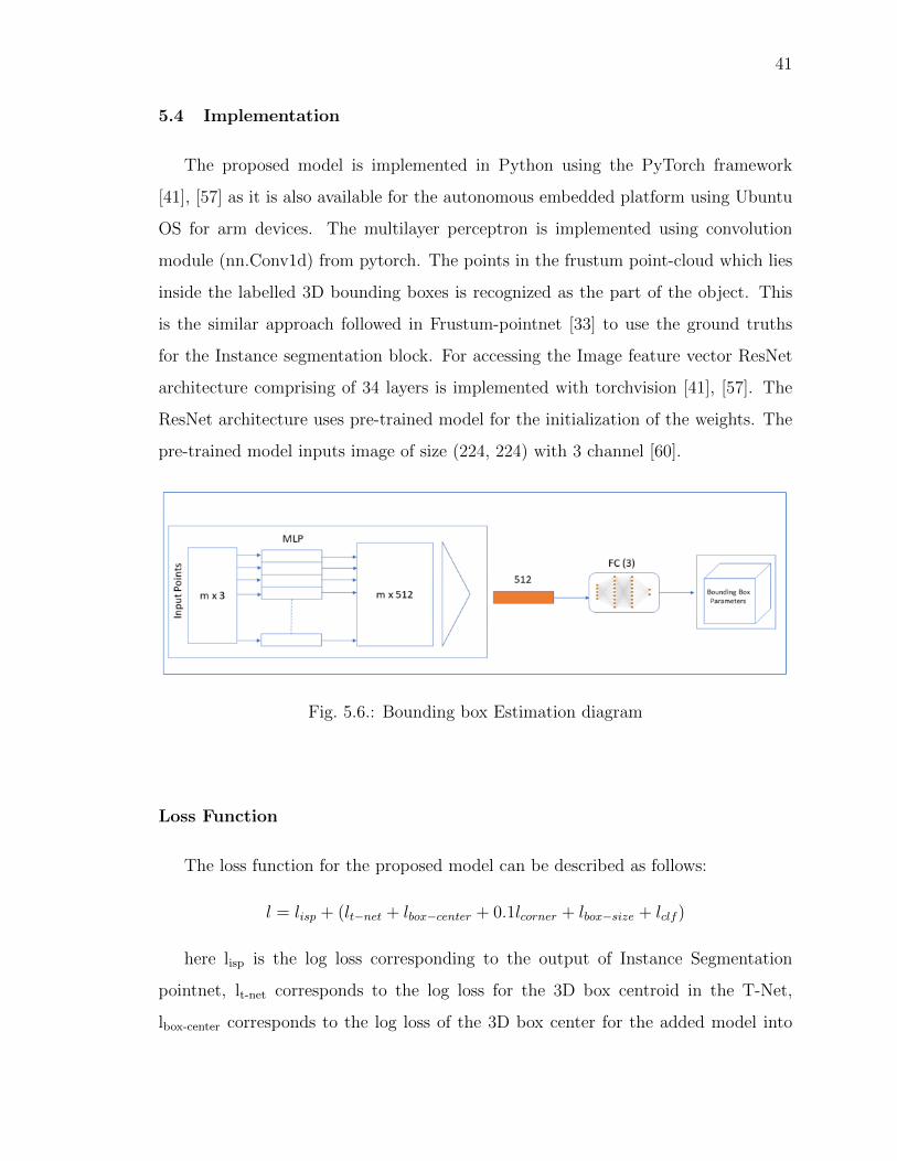
5.6 Bounding box Estimation diagram . . . . . . . . . . . . . . . . . . . . . . 41
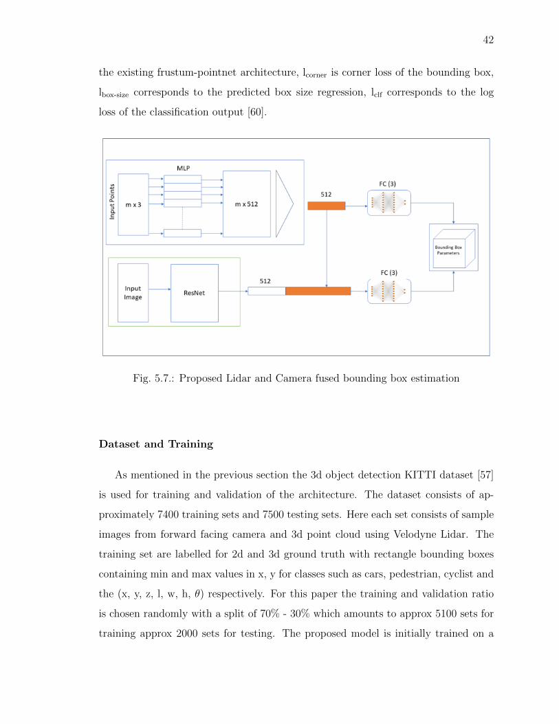
5.7 Proposed Lidar and Camera fused bounding box estimation . . . . . . . . 42
5.8 Validation precision score curve on KITTI dataset . . . . . . . . . . . . . . 44
5.9 Validation accuracy curve on KITTI dataset . . . . . . . . . . . . . . . . . 45
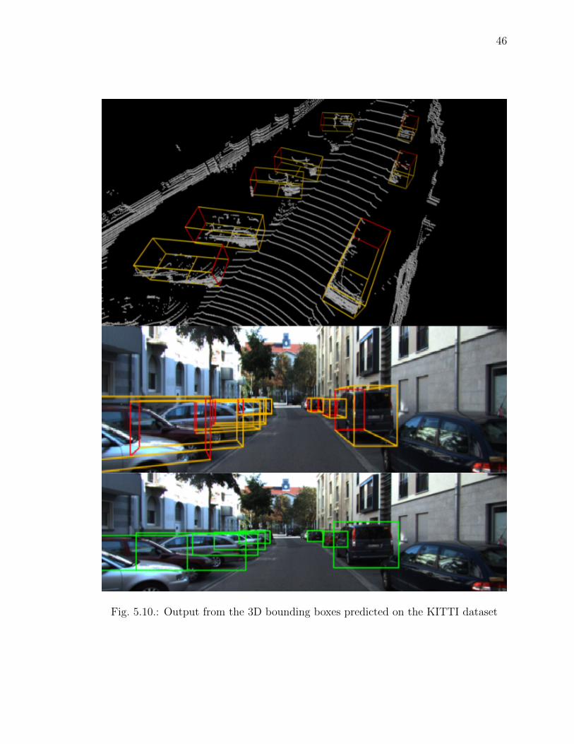
5.10 Output from the 3D bounding boxes predicted on the KITTI dataset . . . 46
6.1 Overview of Hardware deployment (BlueBox 2.0 and RTMaps). . . . . . . 49
6.2 Architecture of Bluebox 2.0 and Sense Think and Act model[Pic CourtesyNXP]. . . . . . . . . . . . . . . . . . . . . . . . . . . . . . . . . . . . . . . 51
6.3 Architecture of BlBX2 [Pic Courtesy NXP]. . . . . . . . . . . . . . . . . . 52
6.4 Architecture of S32V234 vision processor [Pic Courtesy NXP]. . . . . . . . 52
6.5 Architecture of LS2084A Processor[Pic Courtesy NXP]. . . . . . . . . . . . 53
6.6 System overview of NXP BlueBox 2.0 BLBX2. . . . . . . . . . . . . . . . . 54
6.7 Hardware deployment of the model using the RTMaps and BlueBox 2.0 . . 56
6.8 Proposed Combined model for BlueBox 2.0. . . . . . . . . . . . . . . . . . 57

x
SYMBOLS
~ Convolution
ri Feature map
C(.) Cost function of the network
xi
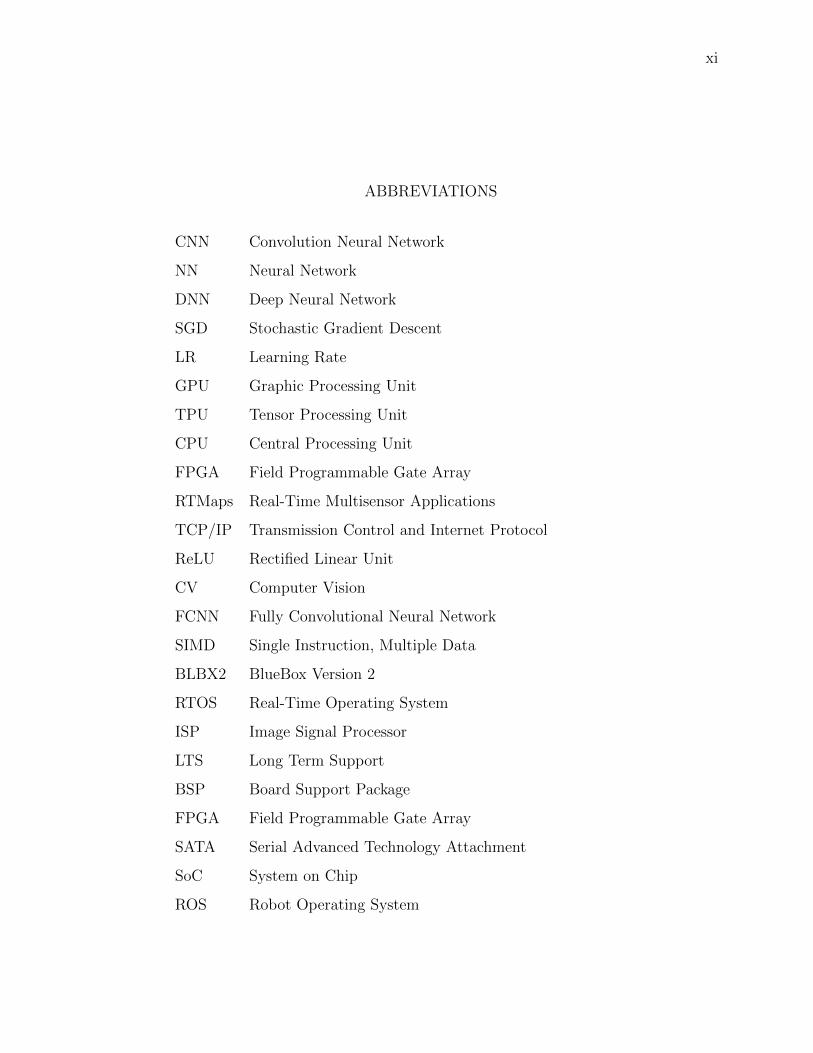
ABBREVIATIONS
CNN Convolution Neural Network
NN Neural Network
DNN Deep Neural Network
SGD Stochastic Gradient Descent
LR Learning Rate
GPU Graphic Processing Unit
TPU Tensor Processing Unit
CPU Central Processing Unit
FPGA Field Programmable Gate Array
RTMaps Real-Time Multisensor Applications
TCP/IP Transmission Control and Internet Protocol
ReLU Rectified Linear Unit
CV Computer Vision
FCNN Fully Convolutional Neural Network
SIMD Single Instruction, Multiple Data
BLBX2 BlueBox Version 2
RTOS Real-Time Operating System
ISP Image Signal Processor
LTS Long Term Support
BSP Board Support Package
FPGA Field Programmable Gate Array
SATA Serial Advanced Technology Attachment
SoC System on Chip
ROS Robot Operating System

xii
ABSTRACT
Katare, Dewant. M.S.E.C.E., Purdue University, December 2019. Exploration ofDeep Learning Applications on An Autonomous Embedded Platform (Bluebox 2.0).Major Professor: Mohamed El-Sharkawy.
An Autonomous vehicle depends on the combination of latest technology or the
ADAS safety features such as Adaptive cruise control (ACC), Autonomous Emergency
Braking (AEB), Automatic Parking, Blind Spot Monitor, Forward Collision Warning
or Avoidance (FCW or FCA), Lane Departure Warning. The current trend follows
incorporation of these technologies using the Artificial neural network or Deep neural
network, as an imitation of the traditionally used algorithms. Recent research in the
field of deep learning and development of competent processors for autonomous or self
driving car have shown amplitude of prospect, but there are many complexities for
hardware deployment because of limited resources such as memory, computational
power, and energy. Deployment of several mentioned ADAS safety feature using
multiple sensors and individual processors, increases the integration complexity and
also results in the distribution of the system, which is very pivotal for autonomous
vehicles.
This thesis attempts to tackle two important adas safety feature: Forward collision
Warning, and Object Detection using the machine learning and Deep Neural Networks
and there deployment in the autonomous embedded platform.
This thesis proposes the following:
1. A machine learning based approach for the forward collision warning system in
an autonomous vehicle.
2. 3-D object detection using Lidar and Camera which is primarily based on Lidar
Point Clouds.

xiii
The proposed forward collision warning model is based on the forward facing au-
tomotive radar providing the sensed input values such as acceleration, velocity and
separation distance to a classifier algorithm which on the basis of supervised learn-
ing model, alerts the driver of possible collision. Decision Tress, Linear Regression,
Support Vector Machine, Stochastic Gradient Descent, and a Fully Connected Neural
Network is used for the prediction purpose.
The second proposed methods uses object detection architecture, which combines
the 2D object detectors and a contemporary 3D deep learning techniques. For this
approach, the 2D object detectors is used first, which proposes a 2D bounding box
on the images or video frames. Additionally a 3D object detection technique is used
where the point clouds are instance segmented and based on raw point clouds density
a 3D bounding box is predicted across the previously segmented objects.

1
1. INTRODUCTION
The number of sensors and ADAS safety feature in a vehicle has been categorically in-
creased in the past years, the latest progression is towards integration of these sensors
with the state-of-the art deep learning architecture based on the sense, think and act
model, which can provide the assistance to the driver or replace a driver by providing
the highest level of autonomy [5]. The highest level of autonomy in a vehicle can be
described as execution of multiple processes, that serves the self driving functionality
from a source point to destination point without any input or control to a vehicle from
the human. Research shows, this highest level of autonomy is achieved by integrat-
ing multiple sensors such as camera, lidar, global navigation satellite system, radar
thus providing the automotive safety feature or the advanced driver assistance system
[13], [18]. The automotive industry is already using several simple and complex adas
features for long time and has resulted in improving the Over-all drivers experience
Fig. 1.1.: Sense, Think and Act Model [Pic Courtesy NXP]
2
with the ultimate objective of providing better road safety. Braking assistance, Lane
Departure Warning, Adaptive cruise control, GPS based navigation are some of the
features which has been used since its introduction, between the year 1990-2000 [6].
The current trend follows incorporation of the deep learning and machine learning
approaches with the autonomous vehicle to provide maximum precision and human
level accuracy. The principle behind these statistically based learning algorithms is to
interpret and understand the drivers surrounding when provided with the impartial
or neutral-data and thus based on the characteristics of the provided input these al-
gorithms classifies or predict an output. Some of the machine learning approach have
already replaced traditionally used algorithms in applications such as vision-based de-
tection, path planning, and recognition of multiple objects and further classification
of them into traffic signs, cars, bicyclists, pedestrian to name few [5], [15]. Although
the deep neural networks counters the above mentioned problems, the deployment
on the microprocessor or the compact embedded system and therefore the computing
related factors cannot be neglected.
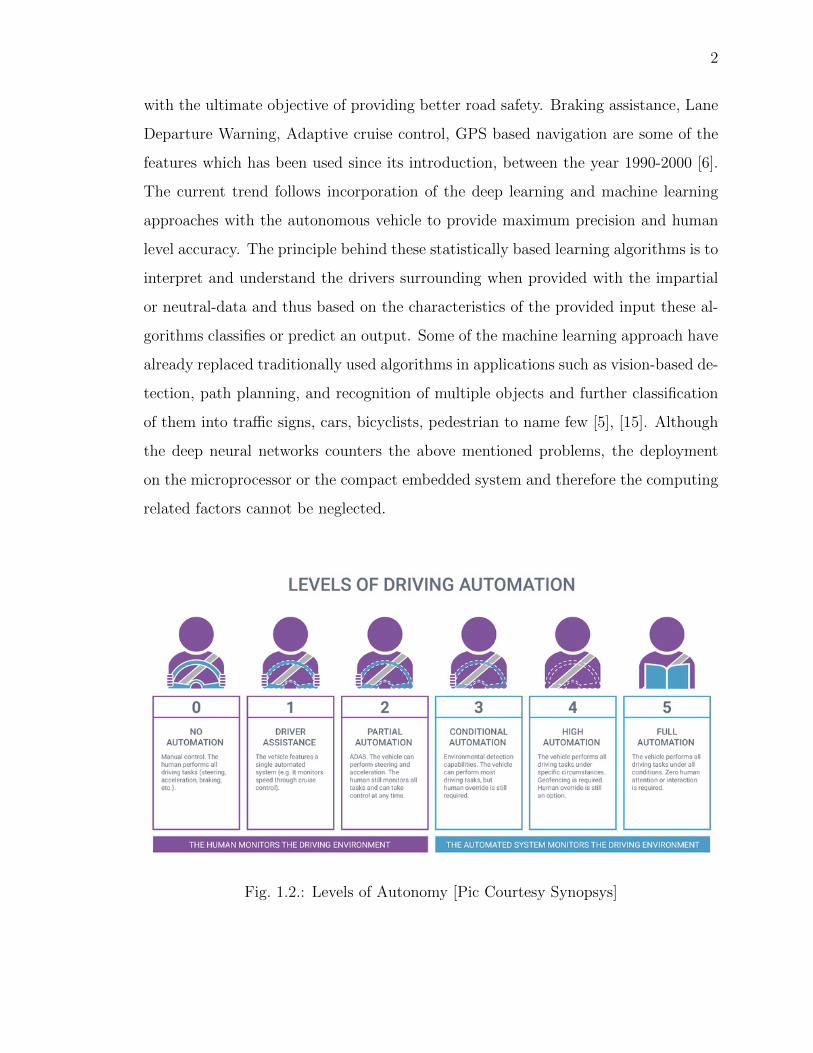
Fig. 1.2.: Levels of Autonomy [Pic Courtesy Synopsys]

3
1.1 Motivation
As mentioned previously the autonomy of vehicle depends on the ADAS features
which are based on the algorithms and the implementation using sensors. The de-
velopment of machine learning and deep neural network architecture predominantly
depends on the data; therefore, it is necessary to have the huge annotated dataset for
the learning of these statistically oriented algorithms. Enormous amount of Image or
video frame related dataset such as CIFAR-10, Imagenet, has been made available
in the past 10 year with the sole purpose of 2d object detection, and advancement
in the GPU computation power has contributed adequately. Some of the well known
2D object detection methods include YOLO [28], Fast R-CNN [30], SSD [29].
Similarly, there has been also increase in collection of instrumented vehicle study
with the purpose of collecting naturalistic driving information recorded with respect
to the road events. One such dataset is 100-car Naturalistic driving data [11], [12]
containing information based on the event such as crash, near-crash and some mis-
cellaneous incidents, the dataset comprises of speed and distance related information
based on the Radar Sensor. However, as mentioned before the self driving vehicle will
consist of multiple sensors connected to a powerful embedded platform comprising of
multiple cores and thus is capable of very fast computation, it is important to address
the applications developed with the inputs of multiple sensors such as Lidar, Camera
and Radar.
Two dimensional object detectors are capable of solving multiple detection and
classification related problems such as traffic sign classifier, lane keeping assistance,
but it fails to map the objects or surrounding around the car in three dimension.
Therefore, there is need of 3D annotated data-set for the development of deep learning
applications. One such dataset is KITTI dataset [26], which comprises of images and
lidar point clouds and 3D annotations. Several machine and deep learning approaches
have been developed and successfully tested to predict and the classify the object.
4
1.2 Research Problem
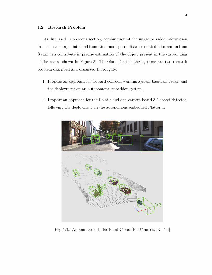
As discussed in previous section, combination of the image or video information
from the camera, point cloud from Lidar and speed, distance related information from
Radar can contribute in precise estimation of the object present in the surrounding
of the car as shown in Figure 3. Therefore, for this thesis, there are two research
problem described and discussed thoroughly:
1. Propose an approach for forward collision warning system based on radar, and
the deployment on an autonomous embedded system.
2. Propose an approach for the Point cloud and camera based 3D object detector,
following the deployment on the autonomous embedded Platform.
Fig. 1.3.: An annotated Lidar Point Cloud [Pic Courtesy KITTI]

5
1.3 Contribution
For the first research problem i.e. the Forward Collision warning system: this
thesis proposes an efficient method to predict a warning or no-warning alert using
the multi-class hidden layer fully connected neural network. During the development
of algorithms several other methods such as Linear Regression, Logistic Regression,
Stochastic Gradient Descent and Support Vector machine were also tried and tested
on the 100-car naturalistic dataset. For the real time application in an embedded and
low power devices the model size and the inference time play a vital role.
For the second research problem i.e. 3D object detection: this thesis proposes a
method to utilize the raw point clouds from the Lidar and process them for object
detection using the instance segmentation. Once an object is detected on the batch of
point clouds, the detected information is further utilized to predict a 3d bounding box
across it. For the authenticity of the 3d detected object in point clouds, a pre-trained
state of the art 2d object detector ”ResNet” is used to detect the object on the video
frames.
This thesis documents the implementation and comparison of above mentioned
methods. Finally, the proposed model is deployed on an autonomous embedded
hardware: BlueBox 2.0, using the RTMaps embedded framework.

6
2. BACKGROUND
This chapter introduces the background and basic fundamentals required for the
implementation of first proposed research statement i.e. Forward Collision Warning
System which is discussed in detail in Chapter 4. The chapter comprises of sections:
Machine Learning, Supervised and Unsupervised Learning, Classification, and the
Artificial Neural Networks.
Definition of Machine Learning:
”A computer program is said to learn from experience E with respect to some class of
tasks T and performance measure P , if its performance at tasks in T , as measured
by P , improves with experience E.” – Dr. Tom M. Mitchell
2.1 Machine Learning
Machine learning has become an important field of computer science, it can be
considered as an abstract of applied statistics where an approach is used to perform
a line of best fit or in other terms, it can be explained as performing a prediction or
classification on the set of data using statistical approach. With the development of
several algorithms and data-sets the Artificial Intelligence system has been provided
with ability to collect and learn extracting patterns or features from the raw data,
and this is known as machine learning. Support Vector Machine and Convolutional
Neural Network are such example, which are generally used as classifier and object
recognition respectively.

7
The primary purpose of using machine learning is to anticipate or predict the out-
come from the unlabeled data, based on the labelled data. The labeled or unlabeled
dataset categorize the machine learning further into the class of supervised learning
or unsupervised learning respectively.
Fig. 2.1.: Supervised Learning [Pic Courtesy Abeyon]
2.2 Supervised Learning
Supervised Learning is the most commonly used class of the machine learning
because of the availability of the dataset. For supervised learning, every content or
index of the dataset is labelled with the some ground truth (right outcome). An
example can be seen from the Figure 2.1 where the dataset consists of images of
labeled cats and they are trained on a supervised learning model. Once the training
is completed the model generates weights containing vital information related to the
classification of the cats based on the ground truth or labeled features. Therefore,
when this predictive binary model is provided with images of cats and other animals
it will classify them into cats and not cats category as shown in the image above.
For a given input variable x and output variable y, after implementing the classi-
fication algorithm the above description can be formally written as:
Y = f(x) (2.1)

8
The primary purpose of the supervised learning approach is to approximate the
above mapping function so that the given input can be mapped to the right class.
Supervised learning is further categorized into classification and regression category.
2.3 Classification
Classification in machine learning is an approach with respect to the given ob-
servation. Here based on the dataset and its pattern, the algorithm tries to fit and
perform the classification on the given set of observation. The simplest form of clas-
sification is a binary classifier, where the observation consists of two classes and a
linear classification approach is utilized to separate them. Another variant of classifi-
cation can be presence of multiple class in the observation set and Supervised form of
machine learning (Support vector machine or logistic regression) is used to separate
and classify the multiple class, the example can be seen in Figure 2.2.
Fig. 2.2.: Types of Classification approach
For the above example with two classes, the line of fit can be given as:
y = f(w,X) = wTX + b (2.2)
Here X is the input vector under observation, w is the weight vector and b is the
bias term, which shifts or adjusts the line of classification.

9
2.4 Artificial Neural Network
In machine learning the Artificial Neural Networks (ANN) are based on the con-
cepts of biological neural network, it falls primarily in the category supervised learn-
ing. For development of model, the Neural Network (NN) is formed by creating the
directed acyclic graph to form a feed-forward neural network. These neurons are
grouped to form layers. Figure 2.3 shows the biological neurons, the main computa-
tional unit of the brain.
As mentioned depending on the requirement a neural network can be organized
in layers and each layer will consists of a number of neurons. These layers can be an
input layer, hidden layer or an output layer. A hidden layer is a layer that is neither
an input nor an output to the network. Depending on the design of the network, there
can be one or several hidden layers. Artificial neurons get the inputs passed from the
x0 or the previous neurons, and then this input is multiplied by weight factor wi to
simulate the interaction. In the later stage these, weighted input signals are summed
up and fixed bias is added, finally this is fed to the non-linear activation function
which gives the output signal. Weights are adjusted according to labels of data to
learn and approximate the inference.
y = f(P [xi × wi] + b) (2.3)
Fig. 2.3.: Biological neuron (left) and its Mathematical model (right).
10
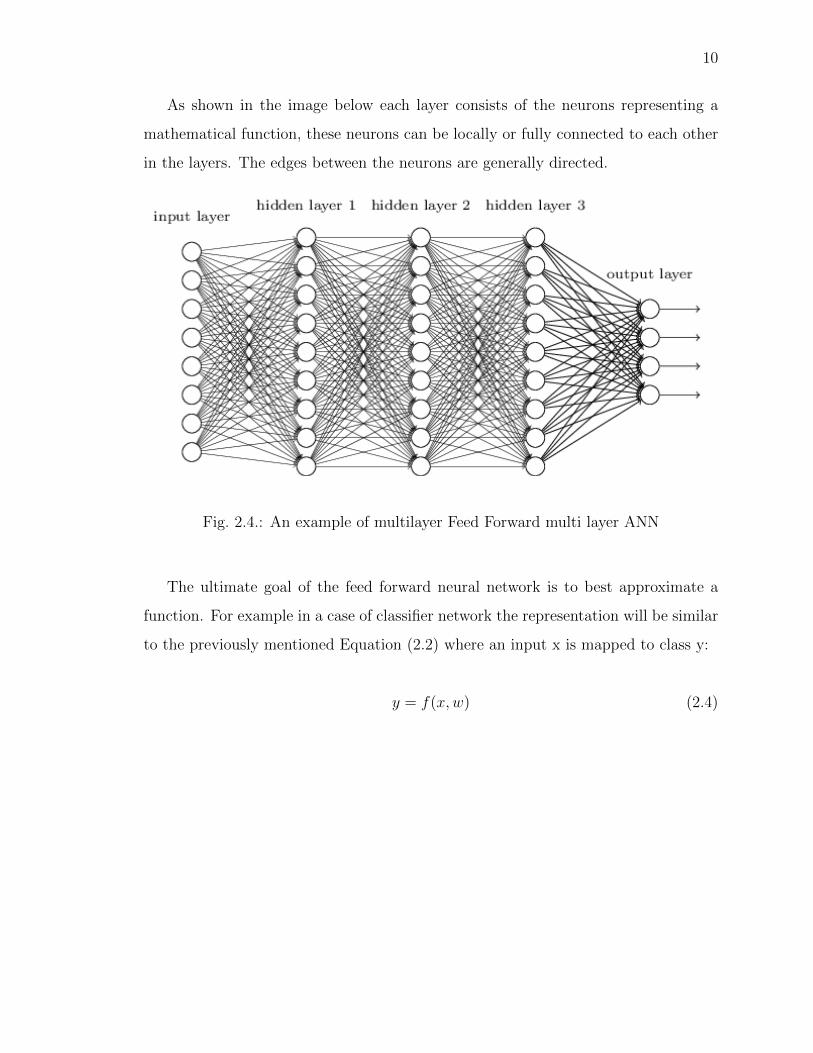
As shown in the image below each layer consists of the neurons representing a
mathematical function, these neurons can be locally or fully connected to each other
in the layers. The edges between the neurons are generally directed.
Fig. 2.4.: An example of multilayer Feed Forward multi layer ANN
The ultimate goal of the feed forward neural network is to best approximate a
function. For example in a case of classifier network the representation will be similar
to the previously mentioned Equation (2.2) where an input x is mapped to class y:
y = f(x,w) (2.4)
11
3. FORWARD COLLISION WARNING ON AN
AUTONOMOUS EMBEDDED SYSTEM
3.1 Introduction
Forward Collision Warning is an advanced driver assistance system or feature that
supervises the speed of the ego vehicle, lead vehicle and the distance between these two
vehicle. Advancement in the latest state of technology with regards to autonomous
vehicle or self driving car ensured the usage of the Forward Collision Warning or
Avoidance (FCW/FCA) System, as one of the most important and the commonly used
active safety feature set, essentially as the prominent crash avoidance system. The
FCW system has already been implemented by several automobile manufacturers in
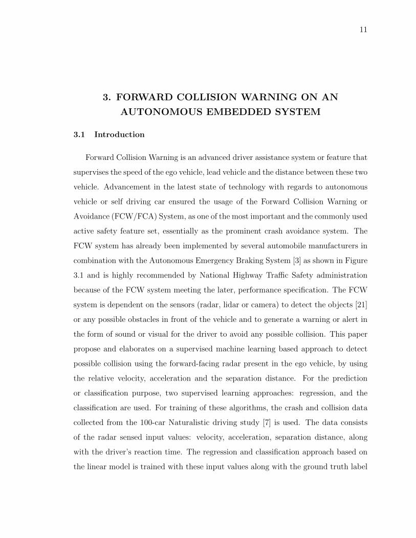
combination with the Autonomous Emergency Braking System [3] as shown in Figure
3.1 and is highly recommended by National Highway Traffic Safety administration
because of the FCW system meeting the later, performance specification. The FCW
system is dependent on the sensors (radar, lidar or camera) to detect the objects [21]
or any possible obstacles in front of the vehicle and to generate a warning or alert in
the form of sound or visual for the driver to avoid any possible collision. This paper
propose and elaborates on a supervised machine learning based approach to detect
possible collision using the forward-facing radar present in the ego vehicle, by using
the relative velocity, acceleration and the separation distance. For the prediction
or classification purpose, two supervised learning approaches: regression, and the
classification are used. For training of these algorithms, the crash and collision data
collected from the 100-car Naturalistic driving study [7] is used. The data consists
of the radar sensed input values: velocity, acceleration, separation distance, along
with the driver’s reaction time. The regression and classification approach based on
the linear model is trained with these input values along with the ground truth label
12
Fig. 3.1.: FCW with Emergency Braking System [38]
and then predicts and classifies the warning or no-warning based on the separation
distance and velocity [38], [43].
3.2 FCW Algorithm
The key behind any FCW system is the warning algorithm [17], [18]. The existing
warning algorithm can be divided into two categories, the kinematic-based and per-
ception based. The Perceptual based algorithm depends on the risk calculating the
factor to present the alert or warning, such as time to a collision that depends on the
data such as the range and speed. However, the kinematic based approach uses the

13
minimum distance required to stop before the collision; therefore, it requires more
detailed data which includes the speed, range, relative deceleration rates and Drivers
reaction time [23]. R. J. Kiefer [11], [12] proposed a kinematic-based FCW algorithm
to calculate the minimum distance needed to stop safely before a collision, under the
Collision Avoidance Metrics Partnership (CAMP) project developed. This algorithm
generates a linear function based on the dynamic parameters to predict the drivers
expected deceleration response based on the last-minute breaking database collected
during the CAMP project. Then proposed Linear equation is by:
Decev = 0.164 + 0.668Declv + 0.00368(Vev − Vlv)2 − 0.078
The generated function is correct for most of the traffic scenario, but may result
in false prediction during the severe risk scenarios [13].
Fig. 3.2.: Proposed method for FCW using Regression Approach

14
3.3 Regression Approach for Prediction
This proposed approach is similar to the CAMPs FCW linear function mentioned
in the previous section. For Regression based prediction the model is trained with the
input data (velocity, acceleration, separation distance) and expected warning range
which leads to the prediction of collision or no-collision warning range. This warning
range when compared with the separation distance leads to the final prediction of the
collision or no-collision alert to notify the driver [38], [43]. The proposed approach is
shown in the Figure 3.2.
Linear Regression
In linear regression, based approach the predicted value (output) is used to iden-
tify the linear relationship with respect to the input values. To identify this linear
relationship, the most important part is to analyze the data and prepare it for the su-
pervised training and then use the data for testing purpose. The next step is to divide
the data into two sets; a bigger ratio of dataset for training purpose and a smaller
ratio of the data set for testing purpose. This prepared dataset is then trained on the
Least Square Fitting model and thus provides an output in the form of scores which
is the coefficient of determination, of the prediction. This models accuracy (Section
3.5), when compared with the CAMPs algorithm was relatively low, as the generated
intercept could not predict the correct warning range based on the expected warning
range and separation distance [38], [43].
3.4 Classification Approach
As the regression-based approach did not result in high accuracy when compared
with the CAMP algorithm, the classification-based approach is used to generate the
model and predict the label for the warning or no-warning scenario. The scikit-
learn [14] module developed for the statistically based machine learning algorithms

15
is used to generate the classifiers based on the artificial neural network, Decision
Tree, Support Vector machine and Stochastic Gradient Descent. The purpose of
any statistical based classification is to use the provided object characteristics and
identify the class or group of the output. The classification approach results in the
prediction based on inputs such as Separation Distance, velocity, acceleration and
Ground Truth Labels (used only for training purpose). The procedure of selecting the
percent size for the training and testing the data is very alike to the Regression based
approach as both falls in the same supervised learning category. The training results
in the generation of a model, which is based on the inputs (velocity, acceleration,
and separation distance) predicts the warning or no-warning scenario by comparing
it with the Ground truth label [38], [43]. The approach is shown in Figure 3.3, The
individual accuracy of the models is discussed in Section 3.5.
Neural Net based classification
Frequently, to model the dataset with higher precision and accuracy, a neural
network based approach can be used to develop a low bias low variance model. The
work-flow of the neural network based classification is very similar to the approach
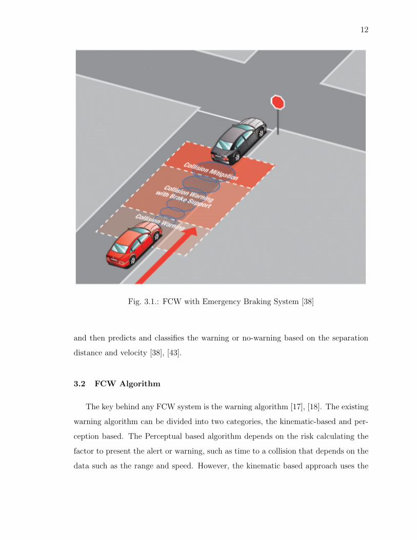
(Figure 3.4) used for DT, SVM and SGD. The proposed neural network is shown
in Figure 3.5. The input parameters for the neural network model are the velocity,
acceleration, and separation distance and based on these inputs the network classifies
the output into one of the two categories: collision warning and no collision warning.
The proposed neural network architecture has 2 hidden layers with 8 neurons in each
layer. The activation function used to model non-linearity in the dataset for each
neuron in the hidden layer is a sigmoid function. The network model has a compact
size with 402 total number of parameters and is deployable on embedded targets such
as NXP Bluebox 2.0 containing Ubuntu-OS and RTMaps framework with the python
programming support [38], [43].

16
Fig. 3.3.: Proposed Classification Approach using supervised learning
3.5 Results
The proposed regression and classification-based approach are first tested on the
RTMaps Studio framework to validate the model and then after initial testing is
deployed on the Bluebox. Since the LS2084 processor provides the maximum available
cores (8 ARM Cortex-A72) for running the RTMaps embedded, it is used for the
deployment. To provide the debug functionality and graphical interface the RTMaps
embedded is shown connected with the RTMaps Studio in the desktop PC (Figure
6.7) using the remote engine connectivity provided over TCP/IP [38], [43].
The standard procedure to make predictions using regression or classification
based approach starts with the finalization of the model. The proposed model is
17
Fig. 3.4.: Proposed Artificial Neural Net classification model for FCW system
trained using the scikit-learn [14] k-fold cross validation and train/test splits of the
data for the regression, classification approach respectively. This practice is preferred
to give an estimate of the performance of the model on the new test-set for example
new data-set. The Figure 7 shows the testing of the regression based approach on
the RTMaps Studio. As seen in the figure the RTMaps consist of the python package
which support the integration of python based programming. The output of the test-
ing result can be seen in the console view. For the classification approach, the model
learns the mapping between the input feature (velocity, acceleration, separation dis-
tance) and the output feature, which is a label (warning or no-warning). The training
and testing of the input variable and the ground truth (labels) were performed on
the different data sizes (varied percent wise). The classification predictions or the

18
output can be categorically divided into the label (classes) and the probability based
prediction. For the SVM classifier the wrong predictions were further divided into
the false positive and false negative. A false positive defines that, the prediction is
related to the collision warning but in real, it is a false alarm or false warning, a false
negative means that the prediction is for the no-collision warning case but in real, it
is a collision warning scenario [38], [43]. This is further shown in the Table 3.1.
Table 3.1.: Table representation of Confusion Matrix for SVM classification
Prediction
Label (Ground Truth)
No Warning Warning
No Threat True Negative False Negative
Threat False Positive True Positive
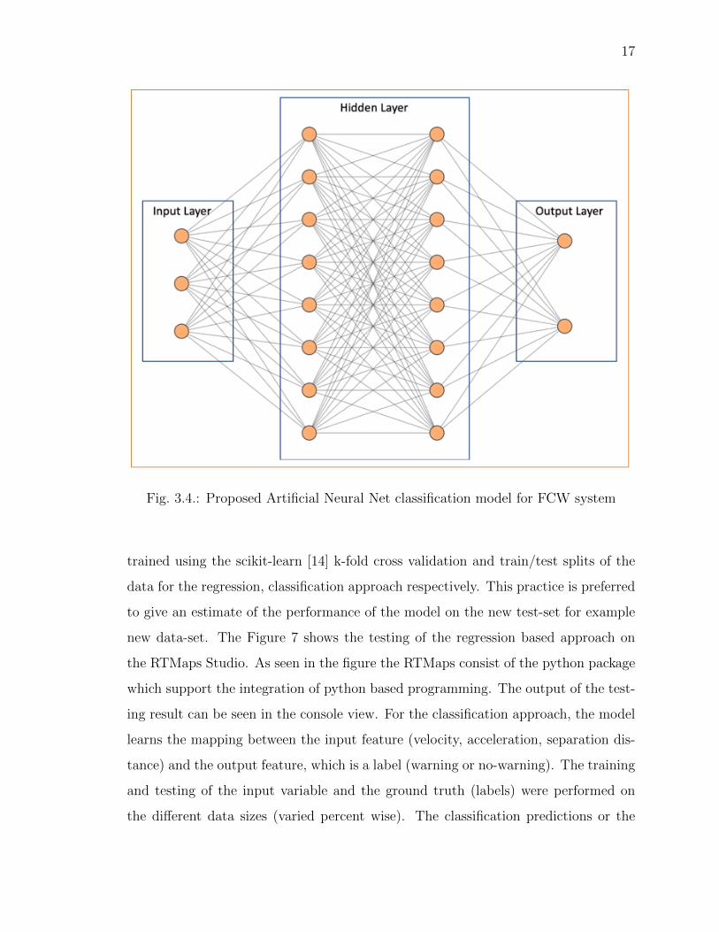
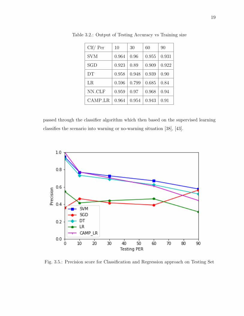
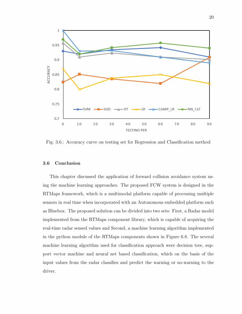
The neural net classifier accuracy ranges around 95-96% with the crash and col-
lision data [7] while the svm classifier ranges around 93-94%. The Figure 3.6, Table
2 shows the accuracy (percentage) of the other classifier and regression model with
respect to the training and testing percent. Among all, the neural network classifier
gave the best accuracy and prediction. It is very apparent that for small size of train-
ing and testing dataset the accuracy is very high, although the comparable factor lies
around the 60-90% of the trained dataset. As mentioned earlier, the RTMaps em-
bedded framework consists of several software module, which can be used to collect
the sensor data. The Figure 8 shows the proposed model based RTMaps diagram,
designed for the collision warning system. The can-frame component module is used
to acquire the sensor data which is then further processed from the radar specific
component module which splits the can bus information into: radar sensed dynamic
parameters such as acceleration, separation distance, velocity, yaw angle, using the
radar specific can bus splitter module. These parameter or sensed inputs is further
19
Table 3.2.: Output of Testing Accuracy vs Training size
Clf/ Per 10 30 60 90
SVM 0.964 0.96 0.955 0.931
SGD 0.923 0.89 0.909 0.922
DT 0.958 0.948 0.939 0.90
LR 0.596 0.799 0.685 0.84
NN CLF 0.959 0.97 0.968 0.94
CAMP LR 0.964 0.954 0.943 0.91
passed through the classifier algorithm which then based on the supervised learning
classifies the scenario into warning or no-warning situation [38], [43].
Fig. 3.5.: Precision score for Classification and Regression approach on Testing Set
20
Fig. 3.6.: Accuracy curve on testing set for Regression and Classification method
3.6 Conclusion
This chapter discussed the application of forward collision avoidance system us-
ing the machine learning approaches. The proposed FCW system is designed in the
RTMaps framework, which is a multimodal platform capable of processing multiple
sensors in real time when incorporated with an Autonomous embedded platform such
as Bluebox. The proposed solution can be divided into two sets: First, a Radar model
implemented from the RTMaps component library, which is capable of acquiring the
real-time radar sensed values and Second, a machine learning algorithm implemented
in the python module of the RTMaps components shown in Figure 6.8. The several
machine learning algorithm used for classification approach were decision tree, sup-
port vector machine and neural net based classification, which on the basis of the
input values from the radar classifies and predict the warning or no-warning to the
driver.

21
4. INSTANTANEOUS SEGMENTATION ON LIDAR
POINT CLOUDS
Related to autonomous vehicle the semantic segmentation can be defined as acquiring
the images or frames from the camera, or the point clouds from the lidar to observe
and interpret the object at the pixel and point level and thus symbolize each of these
label into substantial categories or classes such as traffic signs, lane, vehicle, pedes-
trians as shown in Figure 1. In deep learning techniques convolution neural network
has achieved exceptional results for pixel based semantic segmentation. The first
significant paper [39] on the image segmentation based the fully convolution neural
network introduced the idea of replacing the fully connected layers by the convolution
layer. The paper also contains the use of interpolation layer in the architecture, which
determines that size of output (segmented image) is the same as the size of input.
Another popular technique in the CNN involved use of deconvolution layer [49] for
semantic segmentation, these deconvolution layer identifies the classes pixel-wise and
finally predict the segmentation mask for these identified classes.
Another popular technique derived from traditionally used methods is the combi-
nation of deep convolutional neural network with the conditional random field [42],
which reduces the imperfect localization of the feature for very precise and accurate
object segmentation. For the 3d point cloud based deep learning Frustum-Pointnet
[33] architecture is presented by Qi et al., which is capable of simultaneous seg-
mentation and 3d bounding box prediction across the object. The execution of the
architecture is based on three steps, which are: frustum proposal, Segmentation and
finally the bounding box estimation, this is discussed in detail in Section III. Another
framework, PointFusion [34] is proposed by Xu et al., which utilizes the Pointnet and
ResNet [36] architecture for passing the frustum and 2D object detector respectively.
These all mentioned deep learning has resulted in remarkable improvement for the

22
Fig. 4.1.: Image Semantic Segmentation [42].
semantic image segmentation. However, the achieved high accuracy is a counterfeit
with respect to its implementation on the autonomous embedded system. The pri-
mary objective of this paper is to propose an efficient framework implemented on the
autonomous embedded platform which solves the problem of classification or object
detection based on the semantic segmentation from the 3D lidar data by integrating
supervised learning and deep learning of the local and global feature vector map from
the 3d point clouds. As mentioned, the proposed method utilizes the predicted 3d
bounding box across the object and performing segmentation on the point features.

23
Fig. 4.2.: Vehicle classification with small CNN.
Algorithms such as RANSAC [40] which is based on plane extraction from 3d
point cloud were successful, however it required high computational power thus mak-
ing them difficult for embedded system deployment. Recent research shows that 3d
point cloud contains ample amount of the local features which can be extracted suc-
cessfully, using convolutional neural network [47], [48]. The Squeezeseg [47] is based
on the squeezenet [50] and is capable of real-time segmentation (as shown in figure
2) with the inclusion of traditional technique: conditional random field to improve
the performance of the segmentation mask. Similarly, the PointSeg architecture is
also based on squeezenet, however with an addition of transforming the raw 3d point
cloud data into a a spherical image and then passing the transformed data to the
architecture. This transformed data contains global and local feature, which can be
extracted by the CNN. The CNN architecture comprised of the fire layer, squeeze
reweighting layer and enlargement layer.
24
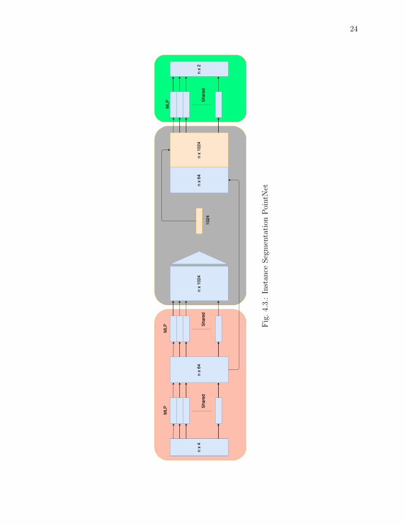
Fig
.4.
3.:
Inst
ance
Seg
men
tati
onP
ointN
et

25
4.1 3D Point cloud Segmentation
The 3d point cloud segmentation is based on the classification and localization of
the points in the 3d plane. The point or pixel wise depth related information of the
object present in the region can be represented in the form of point cloud in the 3d
coordinate. A 3d frustum of the region can be obtained in the form of the projection
matrix. If the camera is integrated with lidar, then the deep learning algorithm
requires the image with depth or the lidar point cloud as an input, and outputs the
3D segmentation for the present objects in the line of sight. The integrated camera
provides the 2d image region and the lidar provides the point cloud through which a
frustum can be proposed which acts as plane to look for the local and global feature
of the present objects in that frustum.
Proposed Model
The proposed model utilizes the frustum point cloud as an input and performs the
binary classification for the points available in the 3d plane, thus predicting whether a
particular point belong to the object, the output is in the form of the probability score.
The proposed model includes an additional feature (Figure 6) exploiting the global
feature from the lidar and output feature of the image from the ResNet architecture.
As shown in Figure 6 the lidar global feature vector is passed as an input to a fully
connected network with five layer, which outputs the centroid position of the 3D
bounding box across the object which is binary classified on the previous step. Also,
the global feature from Lidar is also connected as an input to the image feature
vector, which is then passed to the another fully connected network with five layers
that outputs the value corresponding to the position estimation of 3D bounding box
(length, width, height and angle). The image feature comprising of 2D bounding box
described above, is the output of the 2D object detection or classification from the
ResNet architecture.

26
Instance Segmentation Pointnet
The Instance Segmentation pointnet is the main building block of the architecture
that uses the extracted frustum point cloud as an input and provides two classification
scores for each of the n input points as an output. As mentioned previously, the output
score is the measure of the predicted probability, which describes if the related point
belongs to the chosen object. This network is a modified or upgraded version of
Pointnet [31]. Very likely to the 2d image segmentation the feature or the points
from another object may overlap with another object, in this case the predicted 3D
bounding box for each object plays a vital role as it separates them. The network
architecture is schematically illustrated in Figure 3.
T-Net
This T-Net proposes the centroid position (x,y,z) of the object from the point
cloud, for the 3D bounding box position. The input to T-net is the object point
cloud but it only utilizes the 3D coordinate points of the each given points. The
block diagram is shown in Figure 5.
4.2 Implementation
The model is implemented in Python programming language using the PyTorch
framework [41], [73] and the point cloud library as the modules can be easily imple-
mented in autonomous embedded platform using Arm Ubuntu OS. In the architec-
ture, the multilayer perceptron layers are implemented using the convolution module
(nn.Conv1d) from pytorch. The points in the frustum point-cloud which lies in-
side the labelled 3D bounding boxes is recognized as the part of the object. This
is the similar approach followed in Frustum-pointnet [33] to use the ground truths
for the Instance segmentation block. For accessing the Image feature vector ResNet
architecture comprising of 34 layers is implemented with torchvision [41], [73]. The

27
ResNet architecture uses pre-trained model for the initialization of the weights. The
pre-trained model inputs image of size (224, 224) with 3 channel.
Loss Function
The loss function for the proposed model can be described as follows:
l = lisp + (lt−net + lbox−center + 0.1lcorner + lbox−size + lclf )
here lisp is the log loss corresponding to the output of Instance Segmentation
pointnet, lt-net corresponds to the log loss for the 3D box centroid in the T-Net,
lbox-center corresponds to the log loss of the 3D box center for the added model into
the existing frustum-pointnet architecture, lcorner is corner loss of the bounding box,
lbox-size corresponds to the predicted box size regression, lclf corresponds to the log
loss of the classification output.
Data Augmentation
One of the most important factor to consider during the training of an architecture
is the right learning of the point clouds, which corresponds to how accurately an
architectures predicted the value correctly matching to the ground truth values. This
situation generally occurs when the architecture or model learns the noise feature
instead of the signal features. For the proposed model the overfitting is avoided by
randomly rotating the labelled data from 3D bounding box and points in the frustum
point cloud, by the angle uniformly sampled around the camera’s Y-axis, and for the
frustum point cloud it is augmented by random sampling a subset of points in the
frustum point cloud.
Optimizer
For optimization of the proposed model, the Adam optimizer is used. The adam
optimizer follows an adaptive learning rate by using the first and second order moment

28
of the gradient to update the weights. The starting learning rate of 0.001 is chosen
as random value along with the batch size of 32 frustum point clouds. After every
50 epochs the learning rate is reduced by half of the previous value. The loss is
calculated for the complete validation set on the completion of an epoch, the training
is stopped once the validation loss shows constant values without major change for
80-100 epochs.
Fig. 4.6.: Validation accuracy curve on KITTI dataset
4.3 Results
The proposed model is trained with CITYscapes, KITTI train and test dataset
[3] and evaluated on KITTI val dataset. This section presents the results for the
trained and tested data. It can be seen from Table I that the proposed model with
the Frustum PointNet implementation has performance close to the baseline model.
Figure 9 shows the predicted segmentation of the vehicle class along with the enclosed
3D bounding boxes from the lidar point cloud, Segmentation from the image point
of view and finally the original view from the camera view. Figure 10 and Figure

29
11 shows the validation accuracy and precision score for the KITTI dataset. After
250 - 310 epochs the architecture outputs constant accuracy and precision score with
minor change, and relatively does not change after 350-390 epochs. The proposed
model performs well in most of the scenarios, however when the view point is on the
turning or edges of the scenario it predicts false bounding boxes thus mixed classes
for the segmentation, because of the false angle assumption. The results with respect
to the KITTI dataset are shown in Table I.
Table 4.1.: Comparison of baseline and proposed model on KITTI dataset
Method Precision Recall
Frustum-Pointnet 76.4 90.92
Proposed Frustum-Pointnet - KITTI 74.80 91.83
Proposed Frustum-Pointnet - KITTI (50%) 81.76 92.86
Fig. 4.7.: Validation precision score curve on KITTI dataset
30
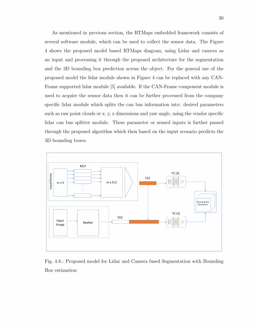
As mentioned in previous section, the RTMaps embedded framework consists of
several software module, which can be used to collect the sensor data. The Figure
4 shows the proposed model based RTMaps diagram, using Lidar and camera as
an input and processing it through the proposed architecture for the segmentation
and the 3D bounding box prediction across the object. For the general use of the
proposed model the lidar module shown in Figure 4 can be replaced with any CAN-
Frame supported lidar module [5] available. If the CAN-Frame component module is
used to acquire the sensor data then it can be further processed from the company
specific lidar module which splits the can bus information into: desired parameters
such as raw point clouds or x, y, z dimensions and yaw angle, using the vendor specific
lidar can bus splitter module. These parameter or sensed inputs is further passed
through the proposed algorithm which then based on the input scenario predicts the
3D bounding boxes.
Fig. 4.8.: Proposed model for Lidar and Camera fused Segmentation with Bounding
Box estimation

31
4.4 Conclusion
This paper proposes an approach to combine the sensed inputs from the Lidar
and camera and then process them through Frustum-pointnet architecture with the
purpose of Segmentation of object present in the line of sight. Here we propose
the Segmentation of the identified point cloud on the basis of defined classes and
finally the prediction of 3D bounding boxes across the detected object from the point
clouds frustum. The proposed detection model is designed in the RTMaps frame-
work, to avail the functionality of real-time detection. The proposed method can be
divided into two parts: first, a Lidar and camera based model implemented from the
RTMaps component library which is capable of acquiring the real-time sensor values
and Secondly, a deep learning algorithm implemented in the python module of the
RTMaps components as shown in Figure 4, which on the basis of the input values
from the lidar and camera classifies, segment and predict the bounding boxes on the
detected vehicle.

32
Fig
.4.
5.:
Pro
pos
edm
odel
for
Blu
ebox
2.0
inth
eR
TM
aps
fram
ewor
kfo
rR
eal
tim
ese
gmen
tati
on
and
bou
ndin
gb
oxpre
dic
tion

33
Fig. 4.9.: Segmentation and the 3D bounding boxes estimation on the KITTI dataset

34
5. 3D BOUNDING BOX DETECTION ON LIDAR POINT
CLOUDS AND VIDEO FRAMES
5.1 Introduction
Localization, Object classification and detection are perception related tasks. Ob-
ject detection can be further divided into 2D detection or 3D, based on cameras,
RGB-D cameras or Lidar respectively. Deep learning based 2D object detection in-
volves drawing of bounding boxes (x, y) around the detected objects in an image or
video frame, whereas the 3D detection involves drawing of three dimensional bound-
ing box (x, y, z) on an object, therefore estimating the exact position of the object
in the 3D plane. Figure 1 shows an example of expected 3D bounding boxes on the
Lidar point cloud and the similar bounding boxes on an image [57]. Deep learning
has been widely accepted as an esteemed technique for image-based computer vision
because of the development of the state of the art convolutional neural network based
architectures [32]. The previous techniques or approach remains the pre-processing of
the 3D point clouds data and adopting them into the data structure required for the
existing deep learning algorithms, thus providing an output based on the algorithm
[36]. Recent researches have proposed to process the Lidar point clouds directly on
deep neural network without converting them to any representations. For example,
[34], [36] proposed different form of deep net architectures, called as Pointnets and
Frustum Pointnets respectively. These deep learning architectures have shown higher
performance and have proved as benchmark for 3D perception based detection such
as object classification and semantic segmentation. Pointnets architecture [31] pro-
posed by Qi et al. is capable of both classification and semantic segmentation of
3d point clouds by learning the local and global feature vector from the raw point
clouds. Zhou et al. presented VoxelNet [34], a deep learning architecture detecting

35
Fig. 5.1.: 3D Vehicle Detection on Lidar Point Clouds and Camera Images [57]
3D bounding boxes based on reading of Lidar Point clouds, here the lidar point clouds
were divided into 3D voxel spaced equally. The architecture successfully detects and
gives high performance for the car, cyclist and pedestrians. The most prominent 3D
object detector Frustum-Pointnet [33] is presented by Qi et al., which predicts the
bounding box on an object based on instance segmentation and the bounding box
estimation. A similar method Pointfusion [34] is proposed by Xu et al. which utilizes
the Pointnet [31] and ResNet [41] architecture for estimating the frustum and a 2D
object detector respectively [60].

36
5.2 2D object Detection
The 2D object detection in an autonomous vehicles are primarily based on the
single or multiple cameras connected to sense the environment or surrounding of the
car. The 2D object detection architecture or algorithm requires the raw image as an
input, and outputs the bounding box with the class or label of the detected object
as shown in figure 2. In 2D object detection the bounding box is an axis-aligned
rectangle, which is almost an exact fit on the position of the multiple objects or
classes in that image, here the bounding box can be parameterized as (xmin, xmax,
ymin, ymax) where (xmin, ymin) are the pixel coordinates of the bottom-left bounding
box corner, and (xmax, ymax) are the pixel coordinates of the top-right corner. An
example of the ground truth 2D bounding boxes from the KITTI dataset [57] is
shown in Figure 2, in which the bounding boxes correspond to the class i.e. car,
traffic light or motorcyclist. Recent State-of-art 2D object detector is based on the
approach where the image is processed on the convolution neural network, extracting
the feature map of the entire image. The selected object regions are passed onto these
extracted feature map, and mapped onto the region feature vector, which on the basis
of the class scores predicts the type of object and proposes the bounding box onto it
[60].
5.3 3D Object Detection
The 3D object detection can be based on the RGB-D cameras, radars, lidar or
combination of such sensors. Here the deep learning algorithm requires the image
with depth information or the lidar point cloud as an input, and outputs the 3D
bounding box for the present objects in the line of sight. A 3D bounding box is very
close to cubical shape covering the objects region on the sensors line of sight. For
automotive applications, a 3D bounding box can be parameterized as (x, y, z, l, w, h,
θ). Here the (x, y, z) is the 3D coordinates of the bounding box center, the (l, w, h) is
length, width and height respectively of the bounding box, and θ is the yaw angle of

37
the bounding box. An example of the ground truth 3D bounding boxes for the vehicle
detection application is shown in Figure 1 from the KITTI dataset [3], where the boxes
are visualized both in the Lidar point cloud along with the respective camera image.
Most of the statistical or deep learning related algorithms for 3D object detection is
however trained and evaluated on the KITTI dataset [57], which contains images and
lidar point clouds collected from the forward facing stereo camera and velodyne Lidar
[60].
Fig. 5.2.: 2D object detection on traffic related data [source: xsens]
As mentioned earlier the Frustum Pointnet architecture comprises of three pri-
mary steps: frustum proposal, instance segmentation and bounding box estimation.
At the frustum proposal step, the 2D proposed region is extruded to extract the cor-
responding 3D frustum proposal, which contains the entire points of the lidar point
cloud, that lies inside the 2D region when it is projected onto the image plane. This
frustum proposal point cloud is then passed to the instance segmentation step, where

38
the PointNet segmentation network carries out the binary classification for each point,
thus predicting if the point is actual part or feature of the detected object. All true
classified points are then passed to the bounding box estimation step, which utilizes
the density of these points to estimate the position of the 3D bounding boxes. To
estimate the center of the bounding box, the model regresses the residuals related to
the segmented point cloud centroid. For the 3d bounding box dimensions and heading
angle, a classification-regression hybrid based approach inspired by Mousavian et al.
[37] is used.
Fig. 5.3.: Instance Segmentation pointnet
Fig. 5.4.: Proposed model for Bluebox 2.0 in the RTMaps framework for Real time
Detection
39
Proposed Model
The model proposed in this paper uses Frustum Pointnet [33] as the base model.
The model contains the Segmentation-Pointnet, Regressed PointNet (T-net), and an
additional feature based on the inputs from the camera for the frustum proposal
based on the known camera projection matrix. The proposed model uses extracted
features from the image, for the position estimation of the 3D bounding boxes. The
proposed model adds another block (Figure 6) exploiting the global feature from the
lidar and output feature vector of the image from the ResNet architecture. As shown
in Figure 6 the lidar global feature vector is passed as an input to a fully connected
network with three layer which outputs the centroid position of the 3D bounding box
w.r.t the center Position estimated by T-net. The same lidar global feature is also
connected as an input to the image feature vector, which is then passed to the another
fully connected network with three layers that outputs the value corresponding to the
position estimation of 3D bounding box (length, width, height and angle). The image
feature comprising of 2D bounding box described above, is the output of the 2D object
detection or classification from the ResNet architecture [60].
Instance Segmentation Pointnet
The Instance Segmentation pointnet uses the extracted frustum point-cloud as an
input and calculates the classification scores for each of the n input points estimating
how probable they belong to the class or object considered for the case or scenario.
The output classification-score is the measure of the predicted probability for a class
among k different classes. For detection of multiple class in a scenario, this network
utilizes the feedback from the 2-D detector: ResNet architecture (Figure 4) for ac-
curate segmentation as it reduces the task of finding similar point cloud densities or
feature, matching the object considered in the scenario. The output from this net-
work combines the global and local feature of the point clouds and segment it on the
basis of category containing predefined maps or vector, for previously mentioned k

40
different classes. This network can be considered as a modified or upgraded version
of Pointnet [60]. The network architecture is schematically illustrated in Figure 3.
T-Net
The input to T-net or Regressed Pointnet architecture (as shown in Figure 5)is
the object point cloud but it only utilizes the 3D coordinate points of the each given
points. The regressed pointnet uses the segmented point clouds from the previous
step and proposes the centroid position (x, y, z) for the chosen point cloud, for the
3D bounding box position. The estimation of the center of the object is performed
here and transformation of the bounding boxes is performed to convert the estimated
center into origin. The bounding box estimation network (as shown in Figure 6) is
based on the regressed pointnet architecture and is similar to T-net with a difference
in the last layer where the outputs are bounding boxes on the segmented objects with
variables: center, size and yaw angle (cx, cy, cz, l, w, h, θ). For the final prediction
of the center and coordinate of the 3D bounding box, the outputs from the bounding
box estimation network (bound-box-est-net) and T-net architecture is combined to
calculate the absolute center on the segmented point cloud as described below.
C = Ct−net + Cbound−box−est−net
Fig. 5.5.: T-net architecture
41
5.4 Implementation
The proposed model is implemented in Python using the PyTorch framework
[41], [57] as it is also available for the autonomous embedded platform using Ubuntu
OS for arm devices. The multilayer perceptron is implemented using convolution
module (nn.Conv1d) from pytorch. The points in the frustum point-cloud which lies
inside the labelled 3D bounding boxes is recognized as the part of the object. This
is the similar approach followed in Frustum-pointnet [33] to use the ground truths
for the Instance segmentation block. For accessing the Image feature vector ResNet
architecture comprising of 34 layers is implemented with torchvision [41], [57]. The
ResNet architecture uses pre-trained model for the initialization of the weights. The
pre-trained model inputs image of size (224, 224) with 3 channel [60].
Fig. 5.6.: Bounding box Estimation diagram
Loss Function
The loss function for the proposed model can be described as follows:
l = lisp + (lt−net + lbox−center + 0.1lcorner + lbox−size + lclf )
here lisp is the log loss corresponding to the output of Instance Segmentation
pointnet, lt-net corresponds to the log loss for the 3D box centroid in the T-Net,
lbox-center corresponds to the log loss of the 3D box center for the added model into
42
the existing frustum-pointnet architecture, lcorner is corner loss of the bounding box,
lbox-size corresponds to the predicted box size regression, lclf corresponds to the log
loss of the classification output [60].
Fig. 5.7.: Proposed Lidar and Camera fused bounding box estimation
Dataset and Training
As mentioned in the previous section the 3d object detection KITTI dataset [57]
is used for training and validation of the architecture. The dataset consists of ap-
proximately 7400 training sets and 7500 testing sets. Here each set consists of sample
images from forward facing camera and 3d point cloud using Velodyne Lidar. The
training set are labelled for 2d and 3d ground truth with rectangle bounding boxes
containing min and max values in x, y for classes such as cars, pedestrian, cyclist and
the (x, y, z, l, w, h, θ) respectively. For this paper the training and validation ratio
is chosen randomly with a split of 70% - 30% which amounts to approx 5100 sets for
training approx 2000 sets for testing. The proposed model is initially trained on a

43
Ubuntu OS desktop pc with intel i7 processor comprising of 32 GB ram and nvidia
GTX 1080 GPU and is finally deployed on NXP Bluebox (an autonomous embedded
system) as described in the next section [60].
Data Augmentation
One of the most important factor to consider during the training of an architecture
is the goodness of fit, which corresponds to how accurately an architectures predicted
value matches to the ground truth values. This situation generally occurs when the
architecture or model learns the noise feature instead of the signal features. For the
proposed model the over-fitting is avoided by randomly rotating the labelled data
from 3D bounding box and points in the frustum point cloud, by the angle uniformly
sampled around the camera’s Y-axis.
Optimizer
For optimization of the proposed model, the Adam optimizer is used. The adam
optimizer follows an adaptive learning rate by using the first and second order moment
of the gradient to update the weights. The starting learning rate of 0.0001 is chosen
as random value along with the batch size of 32 frustum point clouds. After every
60 epochs the learning rate is reduced by half of the previous value. The loss is
calculated for the complete validation set on the completion of an epoch, the training
is stopped once the validation loss shows constant values without major change for
60-100 epochs [60].
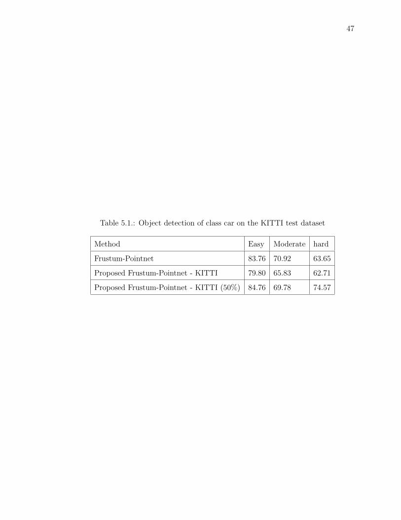
5.5 Results
The proposed model as mentioned in section III and IV is trained with KITTI
train and KITTI test dataset [57] and evaluated on KITTI val dataset. This section
presents the results for the trained and tested data. As shown in Table I, the proposed
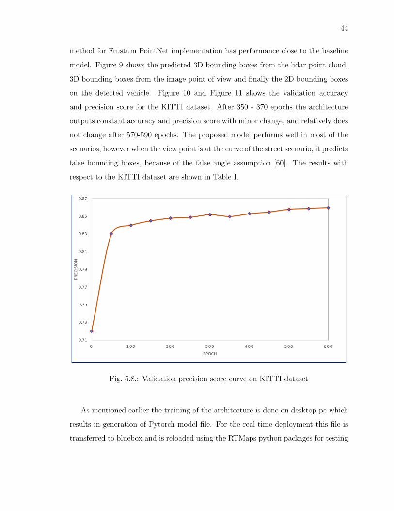
44
method for Frustum PointNet implementation has performance close to the baseline
model. Figure 9 shows the predicted 3D bounding boxes from the lidar point cloud,
3D bounding boxes from the image point of view and finally the 2D bounding boxes
on the detected vehicle. Figure 10 and Figure 11 shows the validation accuracy
and precision score for the KITTI dataset. After 350 - 370 epochs the architecture
outputs constant accuracy and precision score with minor change, and relatively does
not change after 570-590 epochs. The proposed model performs well in most of the
scenarios, however when the view point is at the curve of the street scenario, it predicts
false bounding boxes, because of the false angle assumption [60]. The results with
respect to the KITTI dataset are shown in Table I.
Fig. 5.8.: Validation precision score curve on KITTI dataset
As mentioned earlier the training of the architecture is done on desktop pc which
results in generation of Pytorch model file. For the real-time deployment this file is
transferred to bluebox and is reloaded using the RTMaps python packages for testing

45
with the point cloud and images from KITTI dataset [60]. The real-time scenario can
be tested using the Lidar and camera sensor as per the model proposed in Figure 4.
Fig. 5.9.: Validation accuracy curve on KITTI dataset
The lidar module shown in Figure 4 can be replaced with any CAN-Frame sup-
ported lidar module [5] available, to use the proposed model as a generic one, in that
case the CAN bus component is used to establish the connection with the sensor
and then the acquired inputs can be processed using the vendor specific lidar module
(as shown in Figure 4) which further splits the CAN frame information into desired
parameters such as: raw point clouds or x, y, z dimensions and yaw angle. These
parameter or sensed inputs is further passed through the proposed algorithm which
then based on the input scenario predicts the 3D bounding boxes [60].
46
Fig. 5.10.: Output from the 3D bounding boxes predicted on the KITTI dataset
47
Table 5.1.: Object detection of class car on the KITTI test dataset
Method Easy Moderate hard
Frustum-Pointnet 83.76 70.92 63.65
Proposed Frustum-Pointnet - KITTI 79.80 65.83 62.71
Proposed Frustum-Pointnet - KITTI (50%) 84.76 69.78 74.57
48
5.6 Conclusion
This paper proposes an approach to combine the sensed inputs from the Lidar
and camera and then process them through Frustum-pointnet architecture with the
purpose of predicting 3D bounding boxes on the detected vehicles. The proposed
detection model is designed in the RTMaps frame-work, to avail the functionality
of real-time detection. The proposed method can be divided into two parts: first,
a Lidar and camera based model implemented from the RTMaps component library
which is capable of acquiring the real-time sensor values and Secondly, a deep learning
algorithm implemented in the python module of the RTMaps components shown in
Figure 4, which on the basis of the input values from the lidar and camera classifies
and predict the bounding boxes on the detected vehicle.
49
6. HARDWARE DEPLOYMENT OF THE MODEL ON
BLUEBOX USING RTMAPS
One of the primary purpose of this thesis is to develop deep neural network based
applications and deploy the proposed models on the autonomous embedded platform
such as Bluebox. In the previous chapters, the proposed model for Forward collision
warning and 3D Object detection is discussed. This chapter focuses on hardware
deployment of the model. The model is initially trained using an Intel i7 processor,
32 GB RAM and GTX 1080 GPU by Nvidia using the PyTorch Framework.
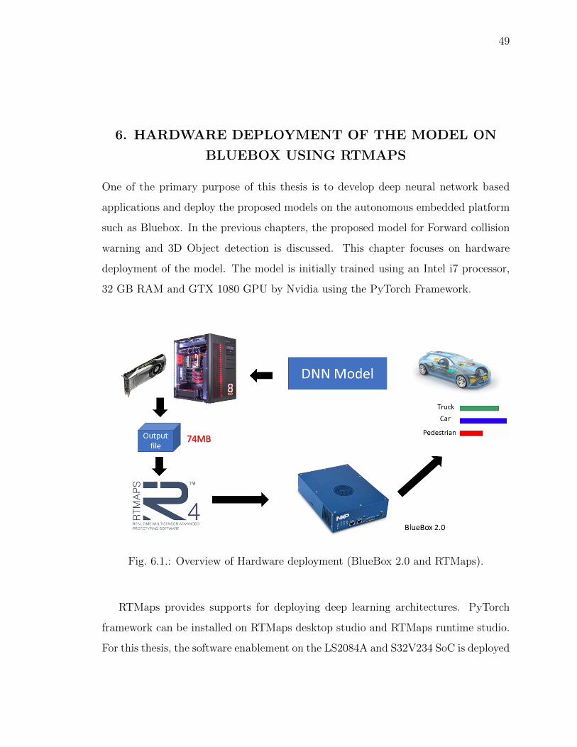
Fig. 6.1.: Overview of Hardware deployment (BlueBox 2.0 and RTMaps).
RTMaps provides supports for deploying deep learning architectures. PyTorch
framework can be installed on RTMaps desktop studio and RTMaps runtime studio.
For this thesis, the software enablement on the LS2084A and S32V234 SoC is deployed

50
using the Linux board support package, which is built using the Yocto framework. The
LS2084A and S32V234 SoC are installed with Ubuntu 16.04 LTS which is a complete,
developer-supported system and contains the complete kernel source code, compilers,
toolchains, with ROS kinetic and Docker package. The deployment overview is shown
in Figure 6.1
6.1 NXP BlueBox
The major challenge in porting an algorithm on the vision system is to optimally
map it to various units of the system in order to achieve an overall boost in the perfor-
mance. This requires detailed knowledge of the individual processors, their capabil-
ities, and limitations. For example, APEX processors are highly parallel computing
units, with Single Instruction Multiple Data (SIMD) architecture, and can handle
data level parallelism quite well. One of the significant requirements of this thesis is
to analyze the capability of NXP Bluebox 2.0 (BLBX2) as an autonomous embedded
system for the real-time applications. Bluebox is one of the development platforms de-
signed for the advanced driver assistance system feature for the autonomous vehicles.
The bluebox development platform is an integrated package for automated driving
and is comprised of three independent systems on chip (SoCs: S32V234, LS2084A,
S32R274) [62], [63].
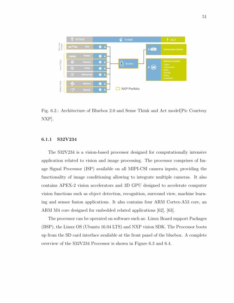
The BLBX2 operates on the independent embedded Linux OS for both the S32V
and LS2 processors, the S32R typically runs bare-metal code or an RTOS. BlueBox
as shown in the Figure 6.2 functions as the central computing unit (as a brain) of the
system thus providing the capability to control the car through actions based on the
inputs collected from the surrounding. This section details the information related to
the components incorporated within the bluebox [62], [63].
51
Fig. 6.2.: Architecture of Bluebox 2.0 and Sense Think and Act model[Pic Courtesy
NXP].
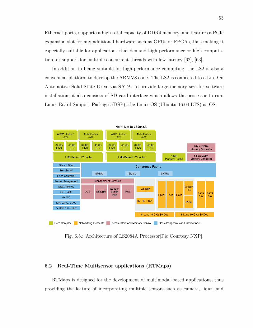
6.1.1 S32V234
The S32V234 is a vision-based processor designed for computationally intensive
application related to vision and image processing. The processor comprises of Im-
age Signal Processor (ISP) available on all MIPI-CSI camera inputs, providing the
functionality of image conditioning allowing to integrate multiple cameras. It also
contains APEX-2 vision accelerators and 3D GPU designed to accelerate computer
vision functions such as object detection, recognition, surround view, machine learn-
ing and sensor fusion applications. It also contains four ARM Cortex-A53 core, an
ARM M4 core designed for embedded related applications [62], [63].
The processor can be operated on software such as: Linux Board support Packages
(BSP), the Linux OS (Ubuntu 16.04 LTS) and NXP vision SDK. The Processor boots
up from the SD card interface available at the front panel of the bluebox. A complete
overview of the S32V234 Processor is shown in Figure 6.3 and 6.4.
52
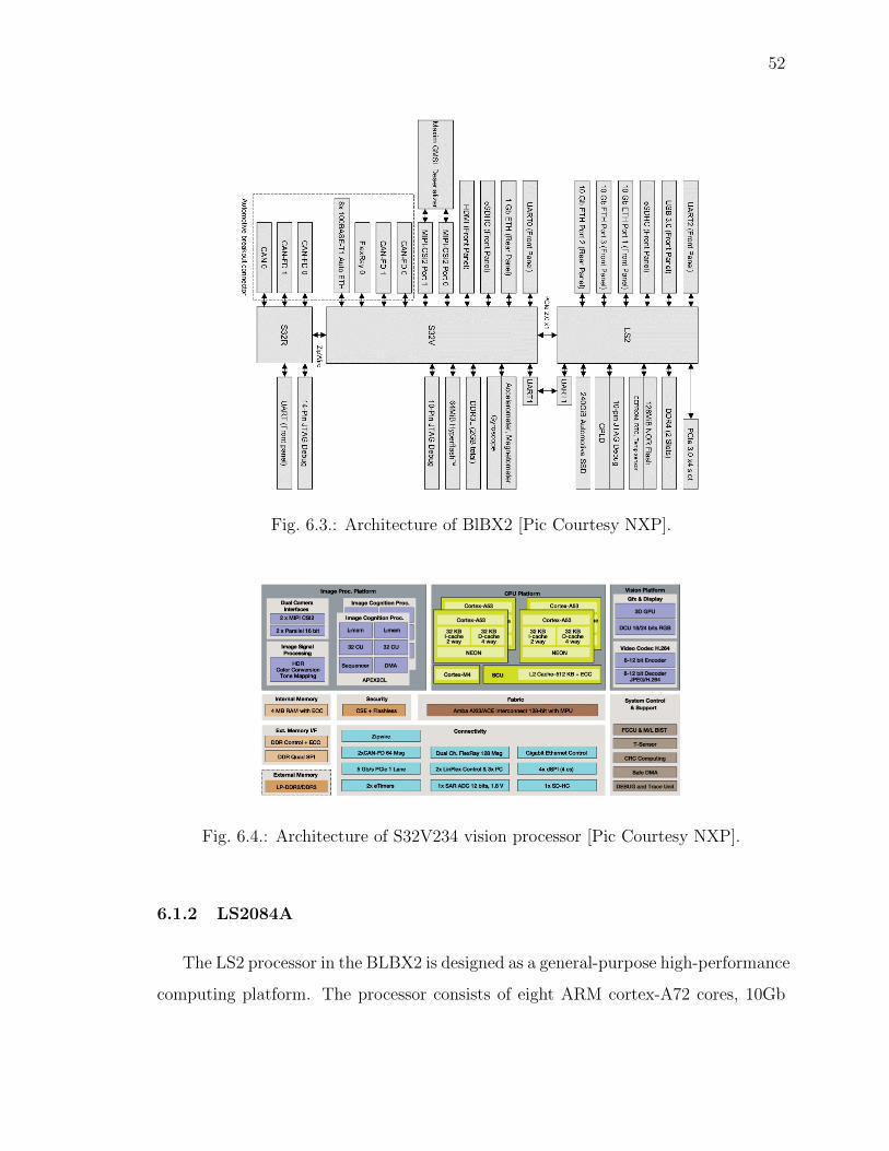
Fig. 6.3.: Architecture of BlBX2 [Pic Courtesy NXP].
Fig. 6.4.: Architecture of S32V234 vision processor [Pic Courtesy NXP].
6.1.2 LS2084A
The LS2 processor in the BLBX2 is designed as a general-purpose high-performance
computing platform. The processor consists of eight ARM cortex-A72 cores, 10Gb
53
Ethernet ports, supports a high total capacity of DDR4 memory, and features a PCIe
expansion slot for any additional hardware such as GPUs or FPGAs, thus making it
especially suitable for applications that demand high performance or high computa-
tion, or support for multiple concurrent threads with low latency [62], [63].
In addition to being suitable for high-performance computing, the LS2 is also a
convenient platform to develop the ARMV8 code. The LS2 is connected to a Lite-On
Automotive Solid State Drive via SATA, to provide large memory size for software
installation, it also consists of SD card interface which allows the processor to run:
Linux Board Support Packages (BSP), the Linux OS (Ubuntu 16.04 LTS) as OS.
Fig. 6.5.: Architecture of LS2084A Processor[Pic Courtesy NXP].
6.2 Real-Time Multisensor applications (RTMaps)
RTMaps is designed for the development of multimodal based applications, thus
providing the feature of incorporating multiple sensors such as camera, lidar, and

54
Fig. 6.6.: System overview of NXP BlueBox 2.0 BLBX2.
radar. It has been tested for processing and fusing the data streams in the real-
time or even in the post-processing scenarios. The software architecture consists of
several independent modules that can be used for different situations and circum-
stances. RTMaps is an asynchronous, high-performance platform to design a mul-
tistory framework and prototype sensor fusion algorithm. RTMaps has of several
modules: RTMaps Runtime Engine, RTMaps Studio, RTMaps Component Library
and RTMaps SDK [37].
6.2.1 RTMaps Runtime Engine
The Runtime Engine is an easily deployable, multi-threaded, highly optimized
module designed in a context to be integrable with third-party applications. Ac-
countable for all base services such as component registration, buffer management,
time stamping threading, and priorities.

55
6.2.2 RTMaps Component Library
It consists of the software module, which is easily interfaceable with the automotive
and other related sensors and packages such as Python, C++, Simulink models, and
3-d viewers, etc. responsible for the development of an application.
6.2.3 RTMaps Studio
It is the graphical modeling environment with the functionality of programming
using Python packages. The development interface is available for the Windows and
Linux based platforms. Applications are developed by using the modules and packages
available from the RTMaps Component library.
6.2.4 RTMaps Embedded
It is a framework which comprises of the component library and the runtime engine
with the capability of running on an embedded x86 or ARM capable platform such as
NXP Bluebox, Raspberry Pi, DSpace MicroAutobox, etc. For this thesis the RTMaps
embedded v4.5.3 platform is tested with NXP Bluebox, it is used independently on the
Bluebox, and with the RTMaps remote studio operating on a computer thus providing
the graphical interface for the development and testing purposes. The connection
between the Computer running RTMaps Remote studio and the Embedded platform
can be accessed via a static TCP/IP as shown in Figure 6.7.

56
6.3 Hardware Implementation
Figure 6.7 shows the process of hardware deployment of the generated model using
RTMaps and BlueBox 2.0. Training is carried at the desktop PC on PyTorch frame-
work and after the successful implementation of 3d object detection algorithms, a final
deploy-able model is generated. RTMaps desktop studio is used to load the model
parameters. TCP/IP connection is established between RTMaps desktop studio and
RTMaps runtime studio using RTMaps runtime engine. Finally, the performance of
the model is evaluated using the BlueBox 2.0.
To evaluate the performance of the model, the video frames of the testing model
are generated using the point cloud library in python to visualise the 3d object detec-
tion in form of lidar frames and camera output. Images shown in the result section
of object detection and segmentation is part of this process.
Fig. 6.7.: Hardware deployment of the model using the RTMaps and BlueBox 2.0
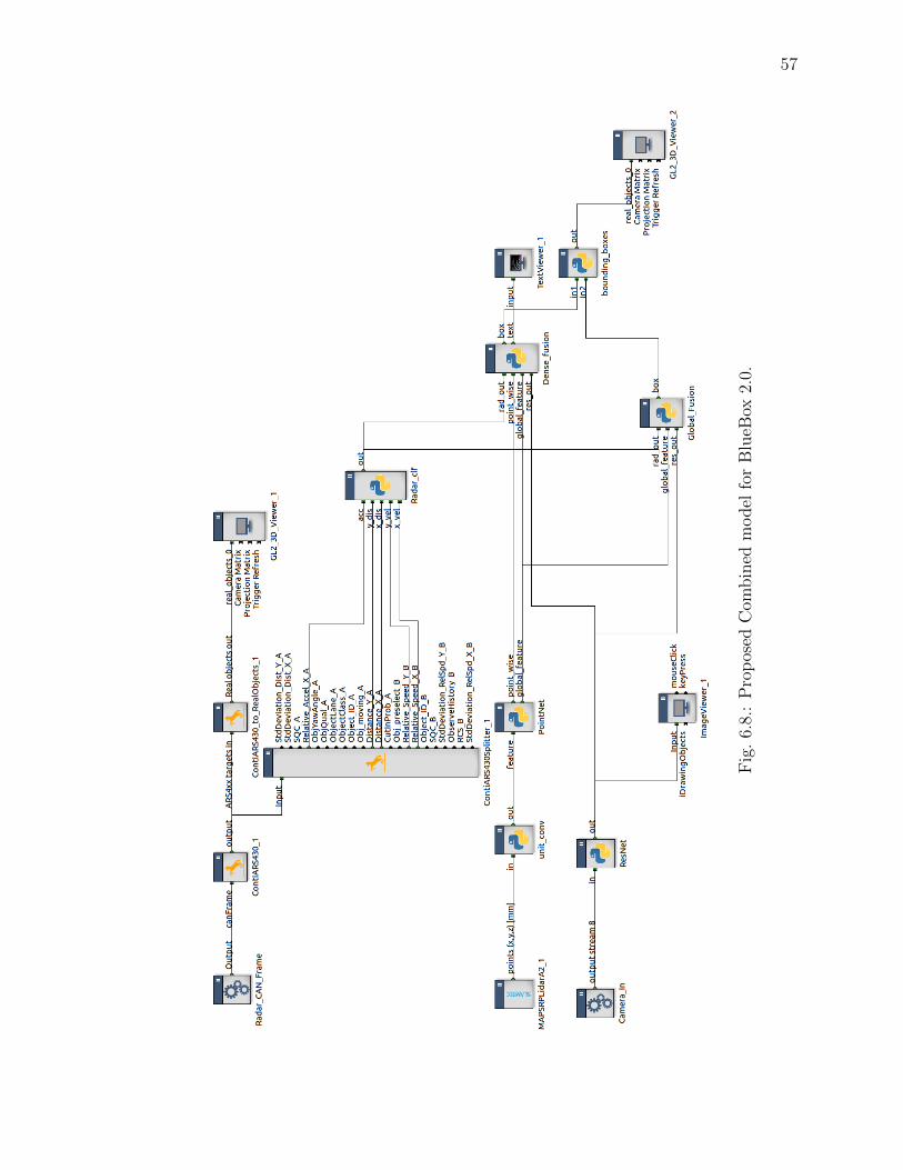
57
Fig
.6.
8.:
Pro
pos
edC
ombin
edm
odel
for
Blu
eBox
2.0.

58
7. SUMMARY
Ample amount of research has been carried out in the field of Perception (detection
and classification) using image or video frames based on deep neural networks. The
major contributions of this thesis can be summarized as follows:
1. Forward Collision Warning System based on ANN Classifier.
2. Instance Segmentation on Lidar Point Clouds using KITTI dataset.
3. 3-D Object detection on Lidar Point clouds and Camera and it’s implementation
on the Autonomous Embedded System.
The FCW proposed Neural Network model achieves 87% accuracy on the 100-car
naturalistic data and outperforms the other tested models such as: Decision Tree, Lin-
ear Regression, Logistic Regression, Stochastic Gradient Descent and Support vector
machine classifier, with reference to the hardware deployment the proposed model can
use the on-board inbuilt radar micro controller S32R274 or the CAN-FRAME con-
nections at LS2084 for connecting the radar sensor and acquiring the required values
through the RTMaps framework and processing it through the proposed algorithm
as mentioned in the Chapter 4.
Similarly, the Object Detection model utilizes the point cloud libraries and camera
frames for the 3d object detection without the conversion or transformation of the
point cloud data. Previous Baseline or state of the art models required conversion
or transformation of raw data before processing it on the deep learning architec-
ture for training and testing, however the proposed model uses the raw point cloud
data for proposing the 3d bounding box with the purpose of object detection for an
autonomous embedded target platform (BlueBox 2.0).

REFERENCES

59
REFERENCES
[1] Cicchino, Jessica B. ”Effectiveness of forward collision warning and autonomousemergency braking systems in reducing front-to-rear crash rates.” Accident Anal-ysis and Prevention 99 (2017): 142-152.
[2] Venkitachalam, Sreeram, ”Realtime Applications with RTMaps and Bluebox2.0.” Proceedings on the International Conference on Artificial Intelligence(ICAI). The Steering Committee of The World Congress in Computer Science,Computer Engineering and Applied Computing (WorldComp), 2018.
[3] Coelingh, Erik, Andreas Eidehall, and Mattias Bengtsson. ”Collision warningwith full auto brake and pedestrian detection-a practical example of automaticemergency braking.” 13th International IEEE Conference on Intelligent Trans-portation Systems. IEEE, 2010.
[4] Vishnukumar, Harsha Jakkanahalli, ”Machine learning and deep neural net-workArtificial intelligence core for lab and real-world test and validation forADAS and autonomous vehicles: AI for efficient and quality test and valida-tion.” 2017 Intelligent Systems Conference (IntelliSys). IEEE, 2017.
[5] Kato, Shinpei, ”Autoware on board: Enabling autonomous vehicles with embed-ded systems.” 2018 ACM/IEEE 9th International Conference on Cyber-PhysicalSystems (ICCPS). IEEE, 2018.
[6] Kuutti, Sampo, ”A survey of the state-of-the-art localization techniques andtheir potentials for autonomous vehicle applications.” IEEE Internet of ThingsJournal 5.2 (2018): 829-846.
[7] Neale, Vicki,”An Overview of the 100-Car Naturalistic Study and Findings.”Proceedings: International Technical Conference on the Enhanced Safety of Ve-hicles. Vol. 2005. National Highway Traffic Safety Administration, 2005.
[8] Song, Wenjie, ”Real-time lane detection and forward collision warning systembased on stereo vision.” Intelligent Vehicles Symposium (IV), 2017 IEEE. IEEE,2017.
[9] Intempora.com. (2018). Intempora - RTMaps An easy-to-use framework for de-velopment of multi-sensor applications. https://intempora.com/ accessed: 2018-09-14
[10] Intempora.com. (2018). Intempora - RTMaps: For multi-sensor applications.https://intempora.com/prducts/rtmaps accessed: 2018-09-14
[11] Kiefer, Raymond, Development and validation of functional definitions and eval-uation procedures for collision warning/avoidance systems. No. DOT-HS-808-964. United States. Department of Transportation. National Highway TrafficSafety Administration, 1999.
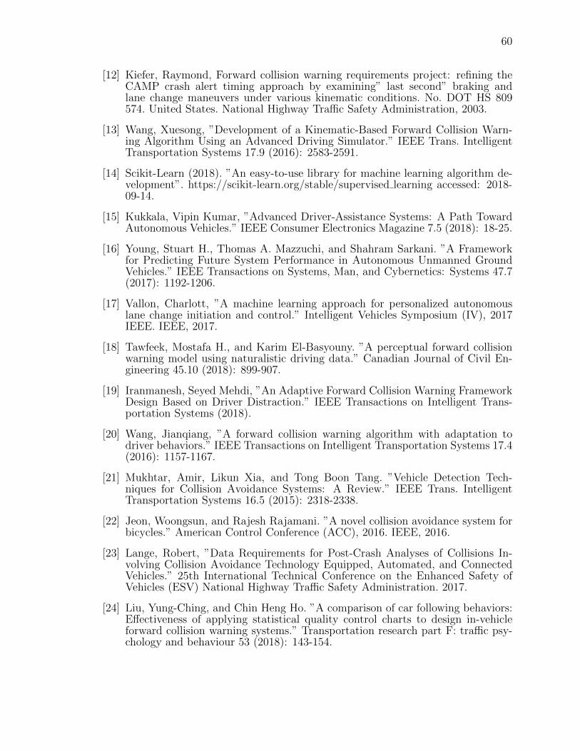
60
[12] Kiefer, Raymond, Forward collision warning requirements project: refining theCAMP crash alert timing approach by examining” last second” braking andlane change maneuvers under various kinematic conditions. No. DOT HS 809574. United States. National Highway Traffic Safety Administration, 2003.
[13] Wang, Xuesong, ”Development of a Kinematic-Based Forward Collision Warn-ing Algorithm Using an Advanced Driving Simulator.” IEEE Trans. IntelligentTransportation Systems 17.9 (2016): 2583-2591.
[14] Scikit-Learn (2018). ”An easy-to-use library for machine learning algorithm de-velopment”. https://scikit-learn.org/stable/supervised learning accessed: 2018-09-14.
[15] Kukkala, Vipin Kumar, ”Advanced Driver-Assistance Systems: A Path TowardAutonomous Vehicles.” IEEE Consumer Electronics Magazine 7.5 (2018): 18-25.
[16] Young, Stuart H., Thomas A. Mazzuchi, and Shahram Sarkani. ”A Frameworkfor Predicting Future System Performance in Autonomous Unmanned GroundVehicles.” IEEE Transactions on Systems, Man, and Cybernetics: Systems 47.7(2017): 1192-1206.
[17] Vallon, Charlott, ”A machine learning approach for personalized autonomouslane change initiation and control.” Intelligent Vehicles Symposium (IV), 2017IEEE. IEEE, 2017.
[18] Tawfeek, Mostafa H., and Karim El-Basyouny. ”A perceptual forward collisionwarning model using naturalistic driving data.” Canadian Journal of Civil En-gineering 45.10 (2018): 899-907.
[19] Iranmanesh, Seyed Mehdi, ”An Adaptive Forward Collision Warning FrameworkDesign Based on Driver Distraction.” IEEE Transactions on Intelligent Trans-portation Systems (2018).
[20] Wang, Jianqiang, ”A forward collision warning algorithm with adaptation todriver behaviors.” IEEE Transactions on Intelligent Transportation Systems 17.4(2016): 1157-1167.
[21] Mukhtar, Amir, Likun Xia, and Tong Boon Tang. ”Vehicle Detection Tech-niques for Collision Avoidance Systems: A Review.” IEEE Trans. IntelligentTransportation Systems 16.5 (2015): 2318-2338.
[22] Jeon, Woongsun, and Rajesh Rajamani. ”A novel collision avoidance system forbicycles.” American Control Conference (ACC), 2016. IEEE, 2016.
[23] Lange, Robert, ”Data Requirements for Post-Crash Analyses of Collisions In-volving Collision Avoidance Technology Equipped, Automated, and ConnectedVehicles.” 25th International Technical Conference on the Enhanced Safety ofVehicles (ESV) National Highway Traffic Safety Administration. 2017.
[24] Liu, Yung-Ching, and Chin Heng Ho. ”A comparison of car following behaviors:Effectiveness of applying statistical quality control charts to design in-vehicleforward collision warning systems.” Transportation research part F: traffic psy-chology and behaviour 53 (2018): 143-154.

61
[25] Elmalaki, Salma, Huey-Ru Tsai, and Mani Srivastava. ”Sentio: Driver-in-the-Loop Forward Collision Warning Using Multisample Reinforcement Learning.”Proceedings of the 16th ACM Conference on Embedded Networked Sensor Sys-tems. ACM, 2018.
[26] Geiger, Andreas, Philip Lenz, and Raquel Urtasun. ”Are we ready for au-tonomous driving? the kitti vision benchmark suite.” 2012 IEEE Conferenceon Computer Vision and Pattern Recognition. IEEE, 2012.
[27] Verbickas, Rytis, ”SqueezeMap: fast pedestrian detection on a low-power auto-motive processor using efficient convolutional neural networks.” Proceedings ofthe IEEE Conference on Computer Vision and Pattern Recognition Workshops.2017.
[28] Redmon, Joseph, ”You only look once: Unified, real-time object detection.”Proceedings of the IEEE conference on computer vision and pattern recognition.2016.
[29] Liu, Wei, ”Ssd: Single shot multibox detector.” European conference on com-puter vision. Springer, Cham, 2016.
[30] Girshick, Ross. ”Fast r-cnn.” Proceedings of the IEEE international conferenceon computer vision. 2015.
[31] Qi, Charles R., ”Pointnet: Deep learning on point sets for 3d classification andsegmentation.” Proceedings of the IEEE Conference on Computer Vision andPattern Recognition. 2017.
[32] Zhou, Yin, and Oncel Tuzel. ”Voxelnet: End-to-end learning for point cloudbased 3d object detection.” Proceedings of the IEEE Conference on ComputerVision and Pattern Recognition. 2018.
[33] Qi, Charles R., ”Frustum pointnets for 3d object detection from rgb-d data.”Proceedings of the IEEE Conference on Computer Vision and Pattern Recogni-tion. 2018.
[34] Xu, Danfei, Dragomir Anguelov, and Ashesh Jain. ”Pointfusion: Deep sensorfusion for 3d bounding box estimation.” Proceedings of the IEEE Conference onComputer Vision and Pattern Recognition. 2018.
[35] Intempora.com. (2018). Intempora - RTMaps: For multi-sensor applications.https://intempora.com/prducts/rtmaps accessed: 2019-03-14
[36] He, Kaiming, ”Deep residual learning for image recognition.” Proceedings of theIEEE conference on computer vision and pattern recognition. 2016.
[37] Mousavian, Arsalan, ”3d bounding box estimation using deep learning and ge-ometry.” Proceedings of the IEEE Conference on Computer Vision and PatternRecognition. 2017.
[38] Katare, Dewant, and Mohamed El-Sharkawy. ”Embedded System Enabled Vehi-cle Collision Detection: An ANN Classifier.” 2019 IEEE 9th Annual Computingand Communication Workshop and Conference (CCWC). IEEE, 2019.
62
[39] Long, Jonathan, Evan Shelhamer, and Trevor Darrell. ”Fully convolutional net-works for semantic segmentation.” Proceedings of the IEEE conference on com-puter vision and pattern recognition. 2015.
[40] Douillard, Bertrand, ”On the segmentation of 3D LIDAR point clouds.” 2011IEEE International Conference on Robotics and Automation. IEEE, 2011.
[41] PyTorch, https://pytorch.org/ accessed: 2019-03-14.
[42] Chen, Liang-Chieh, ”Deeplab: Semantic image segmentation with deep convolu-tional nets, atrous convolution, and fully connected crfs.” IEEE transactions onpattern analysis and machine intelligence 40.4 (2018): 834-848.
[43] Katare, Dewant, and Mohamed El-Sharkawy. ”Collision warning system: embed-ded enabled (RTMaps with NXP BLBX2).” 2018 IEEE International Symposiumon Signal Processing and Information Technology (ISSPIT). IEEE, 2018.
[44] Leutenegger, Stefan, Margarita Chli, and Roland Siegwart. ”BRISK: Binary ro-bust invariant scalable keypoints.” 2011 IEEE international conference on com-puter vision (ICCV). Ieee, 2011.
[45] Dalal, Navneet, and Bill Triggs. ”Histograms of oriented gradients for humandetection.” 2005.
[46] Rosten, Edward, and Tom Drummond. ”Fusing points and lines for high perfor-mance tracking.” ICCV. Vol. 2. 2005.
[47] Wu, Bichen, ”Squeezeseg: Convolutional neural nets with recurrent crf for real-time road-object segmentation from 3d lidar point cloud.” 2018 IEEE Interna-tional Conference on Robotics and Automation (ICRA). IEEE, 2018.
[48] Wang, Yuan, ”Pointseg: Real-time semantic segmentation based on 3d lidarpoint cloud.” arXiv preprint arXiv:1807.06288 (2018).
[49] Noh, Hyeonwoo, Seunghoon Hong, and Bohyung Han. ”Learning deconvolutionnetwork for semantic segmentation.” Proceedings of the IEEE international con-ference on computer vision. 2015.
[50] Iandola, Forrest N., ”SqueezeNet: AlexNet-level accuracy with 50x fewer param-eters and¡ 0.5 MB model size.” arXiv preprint arXiv:1602.07360 (2016).
[51] Chen, Xiaozhi, ”Monocular 3d object detection for autonomous driving.” Pro-ceedings of the IEEE Conference on Computer Vision and Pattern Recognition.2016.
[52] Zheng, Shuai, ”Conditional random fields as recurrent neural networks.” Pro-ceedings of the IEEE international conference on computer vision. 2015.
[53] Long, Jonathan, Evan Shelhamer, and Trevor Darrell. ”Fully convolutional net-works for semantic segmentation.” Proceedings of the IEEE conference on com-puter vision and pattern recognition. 2015.
[54] Liu, Wei, ”Ssd: Single shot multibox detector.” European conference on com-puter vision. Springer, Cham, 2016.

63
[55] Paszke, Adam, ”PyTorch: An imperative style, high-performance deep learninglibrary.” Advances in Neural Information Processing Systems. 2019.
[56] NXP Semiconductors,https://www.nxp.com/applications/solutions/automotiveaccessed: 2019-03-14.
[57] Geiger, Andreas, Philip Lenz, and Raquel Urtasun. ”Are we ready for au-tonomous driving? the kitti vision benchmark suite.” 2012 IEEE Conferenceon Computer Vision and Pattern Recognition. IEEE, 2012.
[58] Verbickas, Rytis, ”SqueezeMap: fast pedestrian detection on a low-power auto-motive processor using efficient convolutional neural networks.” Proceedings ofthe IEEE Conference on Computer Vision and Pattern Recognition Workshops.2017.
[59] Han, Song, ”EIE: efficient inference engine on compressed deep neural network.”2016 ACM/IEEE 43rd Annual International Symposium on Computer Architec-ture (ISCA). IEEE, 2016.
[60] Katare, Dewant, and Mohamed El-Sharkawy. ”Autonomous Embedded SystemEnabled 3-D Object Detector:(with Point Cloud and Camera).” 2019 IEEE In-ternational Conference of Vehicular Electronics and Safety (ICVES). IEEE, 2019.
[61] Manghat, Surya Kollazhi, and Mohamed El-Sharkawy. ”Forward Collision Pre-diction with Online Visual Tracking.” 2019 IEEE International Conference ofVehicular Electronics and Safety (ICVES). IEEE, 2019.
[62] Pathak, Durvesh, and Mohamed El-Sharkawy. ”Architecturally CompressedCNN: An Embedded Realtime Classifier (NXP Bluebox2. 0 with RTMaps).”2019 IEEE 9th Annual Computing and Communication Workshop and Confer-ence (CCWC). IEEE, 2019.
[63] Gaikwad, Akash Sunil, and Mohamed El-Sharkawy. ”Pruning convolution neuralnetwork (squeezenet) using taylor expansion-based criterion.” 2018 IEEE Inter-national Symposium on Signal Processing and Information Technology (ISSPIT).IEEE, 2018.
[64] Intempora.com. (2018). Intempora - RTMaps: For multi-sensor applications.https://intempora.com/prducts/rtmaps accessed: 2019-03-14
[65] Girshick, Ross, ”Rich feature hierarchies for accurate object detection and se-mantic segmentation.” Proceedings of the IEEE conference on computer visionand pattern recognition. 2014.
[66] Chen, Liang-Chieh, ”Encoder-decoder with atrous separable convolution for se-mantic image segmentation.” Proceedings of the European conference on com-puter vision (ECCV). 2018.
[67] Wang, Panqu, ”Understanding convolution for semantic segmentation.” 2018IEEE winter conference on applications of computer vision (WACV). IEEE, 2018.
[68] Marmanis, Dimitrios, ”Classification with an edge: Improving semantic imagesegmentation with boundary detection.” ISPRS Journal of Photogrammetry andRemote Sensing 135 (2018): 158-172.
64
[69] Kukkala, Vipin Kumar, ”Advanced Driver-Assistance Systems: A Path TowardAutonomous Vehicles.” IEEE Consumer Electronics Magazine 7.5 (2018): 18-25.
[70] Chen, Liang-Chieh, ”Masklab: Instance segmentation by refining object detec-tion with semantic and direction features.” Proceedings of the IEEE Conferenceon Computer Vision and Pattern Recognition. 2018.
[71] Braun, Markus, ”EuroCity persons: a novel benchmark for person detection intraffic scenes.” IEEE transactions on pattern analysis and machine intelligence(2019).
[72] Redmon, Joseph, and Ali Farhadi. ”YOLO9000: better, faster, stronger.” Pro-ceedings of the IEEE conference on computer vision and pattern recognition.2017.
[73] Chen, Xiaozhi, ”3d object proposals for accurate object class detection.” Ad-vances in Neural Information Processing Systems. 2015.
[74] Russakovsky, Olga, ”Imagenet large scale visual recognition challenge.” Interna-tional journal of computer vision 115.3 (2015): 211-252.