Exploratory Data Analysis!1D!

!

In your mat219_class project1.  CopycodefromD2LtodownloadtheDa7ngProfilesDataset&the

TopMoviesDataset,andrunbothintheConsole.2.  CreateanewRscriptorRnotebookcallededa_1d3.  Includethiscodeinyourscriptornotebook:

library(tidyverse)

diamonds <- ggplot2::diamondsdating_profiles <- read_csv(”dating_profiles.csv”)top_movies <- read_csv(”top_movies.csv")

philosophical view

What is EDA?• ParaphrasingJohnTukey:Itis•  amindset(awillingnesstolookforwhatcanbeseen,whetheror

notitisan7cipated),

•  aflexibility(letthedataspeakforthemselves,explorelotsofavenues)

•  Awaytomakepictures(thepicture-examiningeyeisthebestfinderwehaveofthewhollyunan7cipated)

more concrete view

What is EDA?

•  Verifyexpectedrela7onshipsactuallyexistinthedata

•  Findunexpectedstructureinthedatathatmustbeaccountedfor

•  Ensuretherightques7onsarebeingasked

•  Generateaddi7onalques7onstobeconsidered

•  Provideabasisforfurtherdatacollec7on

There is a large emphasis on graphical exploration because it is the best way to reveal unanticipated structure. We want to•  plot the raw data•  plot simple statistics•  position objects and plots to maximize

pattern recognition

one categorical variable

We examine a categorical variable by looking at counts

diamonds

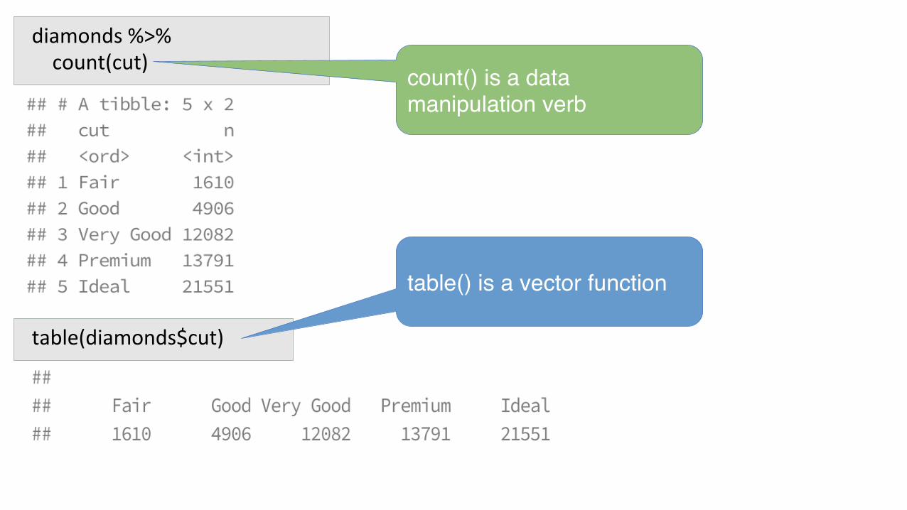
diamonds%>%count(cut)

table(diamonds$cut)

table() is a vector function

count() is a data manipulation verb

da7ng_profiles%>%count(educa7on,sort=TRUE)%>%mutate(pct=100*n/sum(n))

da7ng_profiles%>%count(educa7on,sort=TRUE)%>%mutate(pct=100*n/sum(n))

Thingstoconsider:1.  Groupsizes2.  Vitalfewvs.trivialmany3.  Missingdata4.  Isthereanaturalordering?5.  Recoding6.  Collapsing7.  Datatype:chrvs.fctvs.ord

da7ng_profiles<-da7ng_profiles%>%mutate(educa7on=fct_explicit_na(educa7on))levels(fct_infreq(da7ng_profiles$educa7on))

Thingstoconsider:1.  Groupsizes2.  Vitalfewvs.trivialmany3.   Missingdata4.  Isthereanaturalordering?5.  Recoding6.  Collapsing7.  Datatype:chrvs.fctvs.ord

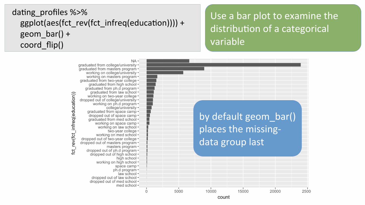
da7ng_profiles%>%ggplot(aes(fct_rev(fct_infreq(educa7on))))+geom_bar()+coord_flip()

Useabarplottoexaminethedistribu7onofacategoricalvariable

da7ng_profiles%>%ggplot(aes(fct_rev(fct_infreq(educa7on))))+geom_bar()+coord_flip()

Useabarplottoexaminethedistribu7onofacategoricalvariable

bydefaultgeom_bar()placesthemissing-datagrouplast

Your Turn 1Consider the pets variable in the dating_profiles dataset. Make a summary of the group counts and make a bar plot. Then, go through the checklist below and think about what you would consider doing.1.  Dogroupsizesvaryalot?2.  Arethereavitalfewand/ortriviallymany?3.  Anymissingdata?4.  Isthereanaturalorderingtothegroups?5.  Shouldweconsiderrecoding/collapsing?

da7ng_profiles%>%mutate(pets=fct_rev(fct_infreq(fct_explicit_na(pets))))%>%ggplot(aes(pets))+geom_bar()+coord_flip()

da7ng_profiles%>%count(pets,sort=TRUE)%>%mutate(pct=100*n/sum(n))

what about pie charts?

Pie charts

Try placing the wedges in order from largest to smallest

Pie charts

Pie charts

What is revealed about the data from this pie chart?

Pie charts

Pie charts

Pie charts are awful because they encode information in angles and areas that are very difficult for humans to judge

Graphics that make comparisons via position on a common scale are best

one numerical variable

We examine a numerical variable by looking at statistical summaries and binned counts (histograms)

diamonds

diamonds%>%summarise(min=min(price),q1=quan7le(price,0.25),median=median(price),mean=mean(price),q3=quan7le(price,0.75),max=max(price))

summary(diamonds$price)

summary() is a generic function

summarise() is a data manipulation verb

diamonds%>%summarise(min=min(price),q1=quan7le(price,0.25),median=median(price),mean=mean(price),q3=quan7le(price,0.75),max=max(price))

summary(diamonds$price)

Thingstoconsider:1.  Whatvaluesaremostcommon?2.  Whichvaluesarerare/extreme?3.  Canyouseeunusualpaherns?4.  Measuresofcenter(mean,

median,etc.)5.  Measuresofspread(std.dev.,

IQR,etc.)6.  Skewness7.  Missingdata

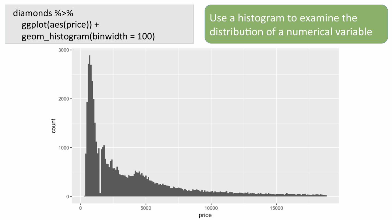
diamonds%>%ggplot(aes(price))+geom_histogram(binwidth=100)

Useahistogramtoexaminethedistribu7onofanumericalvariable

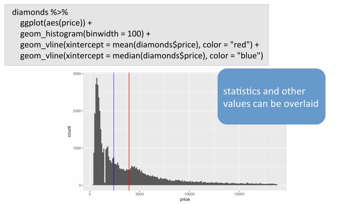
diamonds%>%ggplot(aes(price))+geom_histogram(binwidth=100)+geom_vline(xintercept=mean(diamonds$price),color="red")+geom_vline(xintercept=median(diamonds$price),color="blue")

sta7s7csandothervaluescanbeoverlaid

histogram examples

diamonds%>%filter(carat<3)%>%ggplot(aes(carat))+geom_histogram(binwidth=0.01)

faithful

summary(faithful$erup7ons)

faithful%>%ggplot(aes(erup7ons))+geom_histogram(binwidth=0.25)

histograms on the density scale

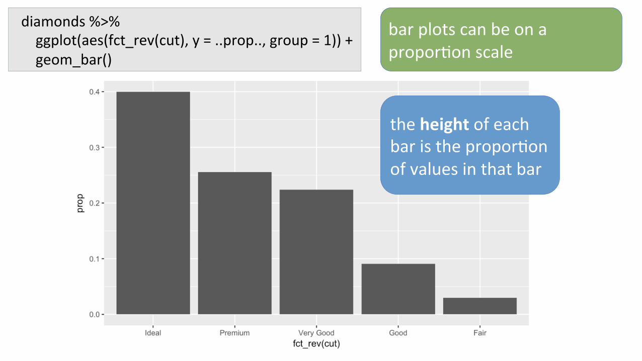
diamonds%>%ggplot(aes(fct_rev(cut),y=..prop..,group=1))+geom_bar()

barplotscanbeonapropor7onscale

theheightofeachbaristhepropor7onofvaluesinthatbar

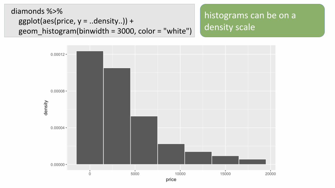
diamonds%>%ggplot(aes(price,y=..density..))+geom_histogram(binwidth=3000,color="white")

histogramscanbeonadensityscale

diamonds%>%ggplot(aes(price,y=..density..))+geom_histogram(binwidth=3000,color="white")

histogramscanbeonadensityscale

theareaofeachbinisthepropor7onofvaluesinthatbin

top_movies%>%ggplot(aes(gross_adj,y=..density..))+geom_histogram(binwidth=100,boundary=300,color="white")

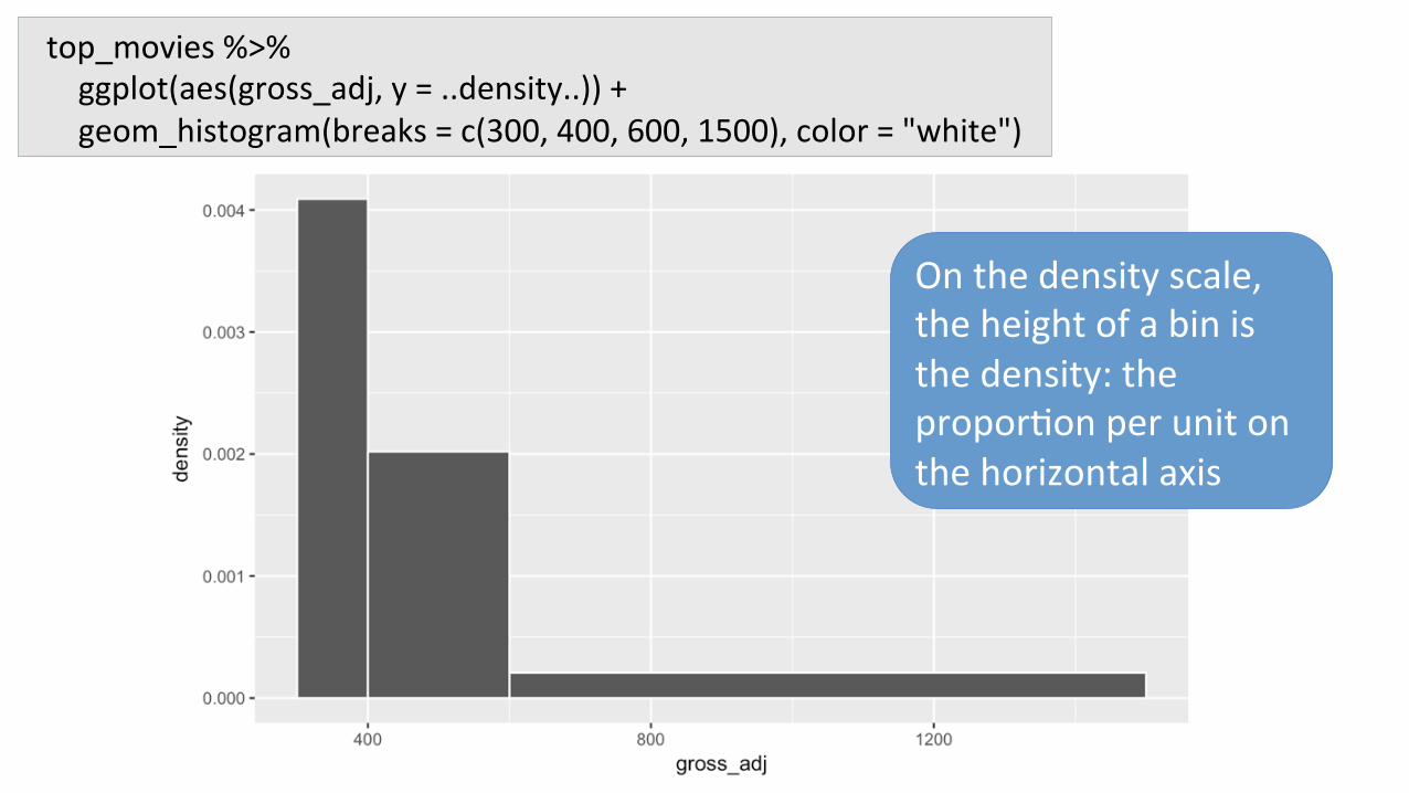
top_movies%>%ggplot(aes(gross_adj,y=..density..))+geom_histogram(breaks=c(300,400,600,1500),color="white")

top_movies%>%ggplot(aes(gross_adj,y=..density..))+geom_histogram(breaks=c(300,400,1500),color="white")

no7cethatthedensityscalereasonablydisplaysthedistribu7on

top_movies%>%ggplot(aes(gross_adj))+geom_histogram(binwidth=100,boundary=300,color="white")

top_movies%>%ggplot(aes(gross_adj))+geom_histogram(breaks=c(300,400,600,1500),color="white")

top_movies%>%ggplot(aes(gross_adj))+geom_histogram(breaks=c(300,400,1500),color="white")

acount(orpropor7on)scalelosestheshapeofthedistribu7on

top_movies%>%ggplot(aes(gross_adj))+geom_histogram(breaks=c(300,400,1500),color="white")

acount(orpropor7on)scalelosestheshapeofthedistribu7on

thisisnotahistogram

top_movies%>%ggplot(aes(gross_adj,y=..density..))+geom_histogram(breaks=c(300,400,600,1500),color="white")

Onthedensityscale,theheightofabinisthedensity:thepropor7onperunitonthehorizontalaxis

top_movies%>%ggplot(aes(gross_adj,y=..density..))+geom_histogram(breaks=c(seq(300,400,by=10),600,1500),color="white")

Onthedensityscale,theheightofabinisthedensity:thepropor7onperunitonthehorizontalaxis

top_movies%>%ggplot(aes(gross_adj,y=..density..))+geom_histogram(breaks=c(300,350,400,450,1500),color="white")

Recap:thereare25moviesrepresentedinthe[400,450)bin,and92inthe[450,1500)bin.Butthelastbinismuchwider,soitislesscrowded(lessdense)

unusual values

ggplot(diamonds)+geom_histogram(aes(y),binwidth=0.5)

ggplot(diamonds)+geom_histogram(mapping=aes(x=y),binwidth=0.5)+coord_cartesian(ylim=c(0,50))

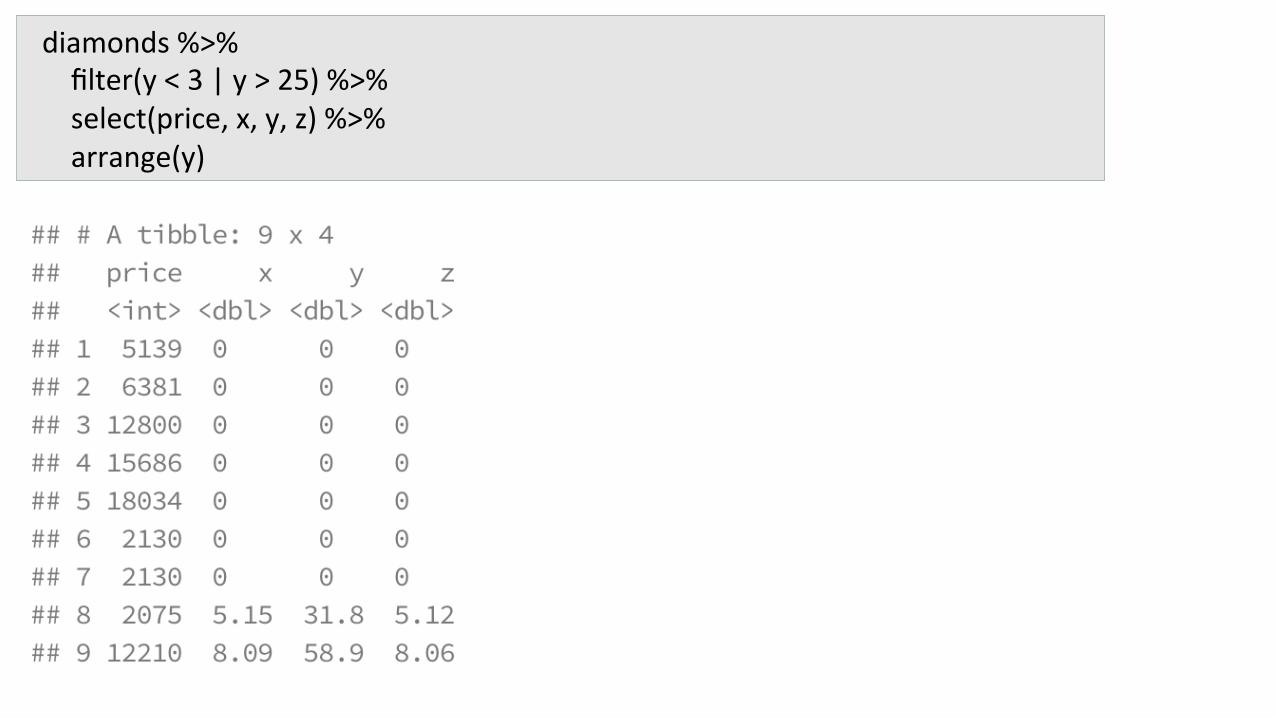
diamonds%>%filter(y<3|y>25)%>%select(price,x,y,z)%>%arrange(y)

diamonds%>%filter(y<3|y>20)%>%select(price,x,y,z)%>%arrange(y)

diamonds2<-diamonds%>%mutate(y=ifelse(y<3|y>20,NA,y))

theunusualdatacanbereplacedwithNA

Your Turn 2Consider the height variable in the dating_profiles dataset. Compute some summary statistics and make a histogram. Do you see any unusual values? Which ones, if any, would you replace with NA

da7ng_profiles%>%ggplot(aes(height))+geom_histogram(binwidth=1)+coord_cartesian(ylim=c(0,20))

missing values

summary(flights$dep_7me)

Firststep:lookforpahernsinthemissingdata.Whatvaluesintheothervariablestendtooccurwiththemissingvalues?Aretherepossibleexplana7onsforthemissingdata?

summary(flights$dep_7me)

Firststep:lookforpahernsinthemissingdata.Whatvaluesintheothervariablestendtooccurwiththemissingvalues?Aretherepossibleexplana7onsforthemissingdata?

Approachestomissingdata:1.  complete-caseanalysis2.  available-caseanalysis3.  imputewiththemean

value4.  imputeusingother

variables5.  converttoacategorical

variableandkeepthemissingdataasanexplicitgroup