Embed Size (px)
Citation preview

1
Exploring The VIX using Automated Trading
Strategies
2
Abstract
This study consists of two major sections: a background analysis of stocks in the biotech
and pharmaceutical industry, and the creation and evaluation of trading strategies. The first
section investigates some technical aspects of historical stock data as well as their correlation
with investor sentiment. This section aims to answer how the Chicago Board Options
Exchange’s volatility index (VIX) can be used to predict stock movement. The second section
covers the creation and evaluation of trading strategies based on the VIX. Software is developed
that dynamically creates different trading methods through simulation. These methods are then
tested over a three month period. Ultimately, the goal of this study is to assess the value of the
VIX as a tool for stock prediction.
3
Table of Contents
Table of Figures .............................................................................................................................. 4
Introduction ..................................................................................................................................... 5
VIX ............................................................................................................................................................. 5
Technical Indicators .................................................................................................................................. 6
Efficient Market Hypothesis ...................................................................................................................... 6
Sample Stocks ................................................................................................................................. 7
Beta ........................................................................................................................................................... 7
Selected Stocks ......................................................................................................................................... 8
General Analysis ........................................................................................................................... 12
Plotting Mean Vs Variance ........................................................................................................... 14
Correlation Matrix ........................................................................................................................ 15
Linear Regression Analysis .......................................................................................................... 16
Plotting Stocks vs the VIX ............................................................................................................ 18
Creating a Trading Program.......................................................................................................... 24
RSI ........................................................................................................................................................... 24
Moving Average ...................................................................................................................................... 25
On Balance Volume ................................................................................................................................. 25
Trading Rules ................................................................................................................................ 26
Simple Moving Average .......................................................................................................................... 26
RSI Rules .................................................................................................................................................. 26
On Balance Volume Rules ....................................................................................................................... 26
Trading Program ........................................................................................................................... 28
Weighting ................................................................................................................................................ 28
Optimizing for Individual Stocks vs All Stocks ......................................................................................... 31
Output ..................................................................................................................................................... 32
Three Month Test .......................................................................................................................... 35
Conclusion .................................................................................................................................... 36
Work Cited .................................................................................................................................... 37
Source Code .................................................................................................................................. 37
4
Table of Figures
Figure 1: General Statistics of Stock Returns ............................................................................... 12
Figure 2: Variance vs Mean Returns ............................................................................................ 14
Figure 3: Correlation Matrix ......................................................................................................... 15
Figure 4: Regression Statistics of Returns vs VIX ....................................................................... 17
Figure 5: IBB vs VIX .................................................................................................................... 18
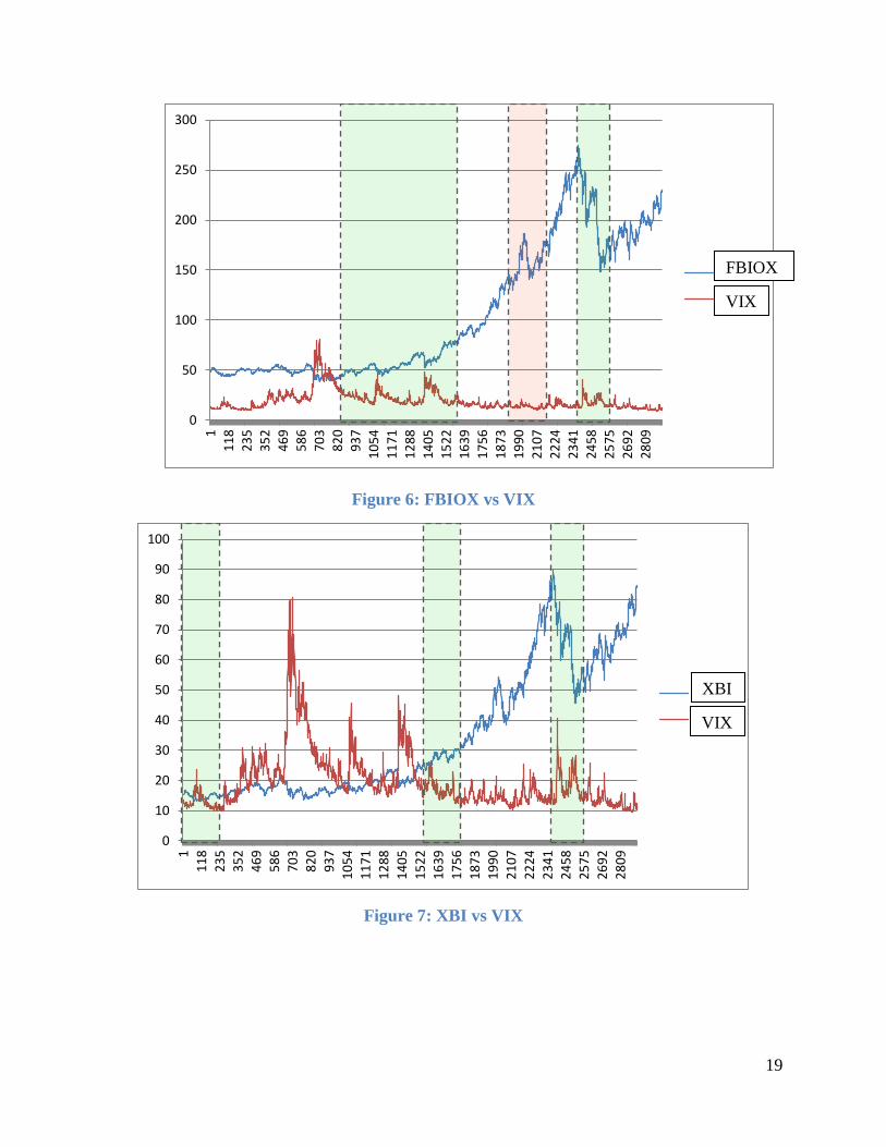
Figure 6: FBIOX vs VIX .............................................................................................................. 19
Figure 7: XBI vs VIX ................................................................................................................... 19
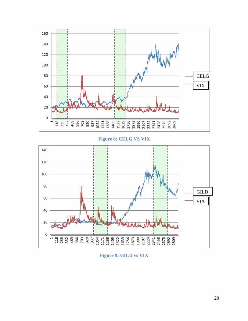
Figure 8: CELG VS VIX .............................................................................................................. 20
Figure 9: GILD vs VIX ................................................................................................................. 20
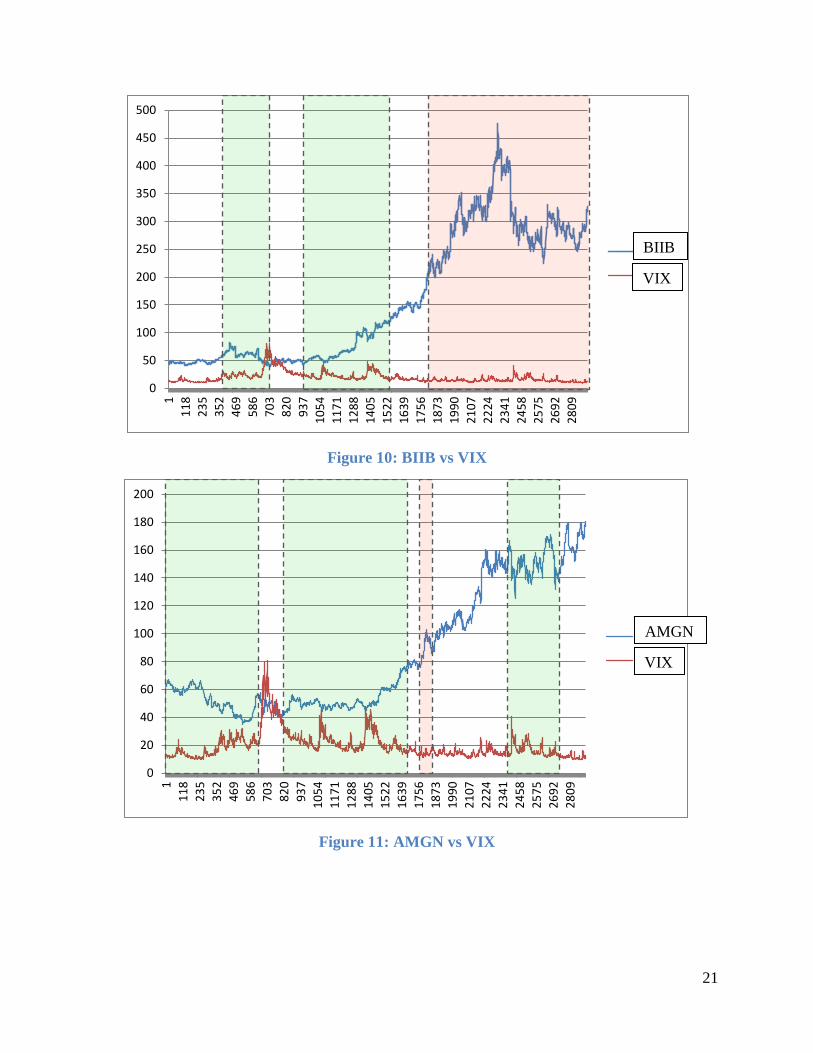
Figure 10: BIIB vs VIX ................................................................................................................ 21
Figure 11: AMGN vs VIX ............................................................................................................ 21
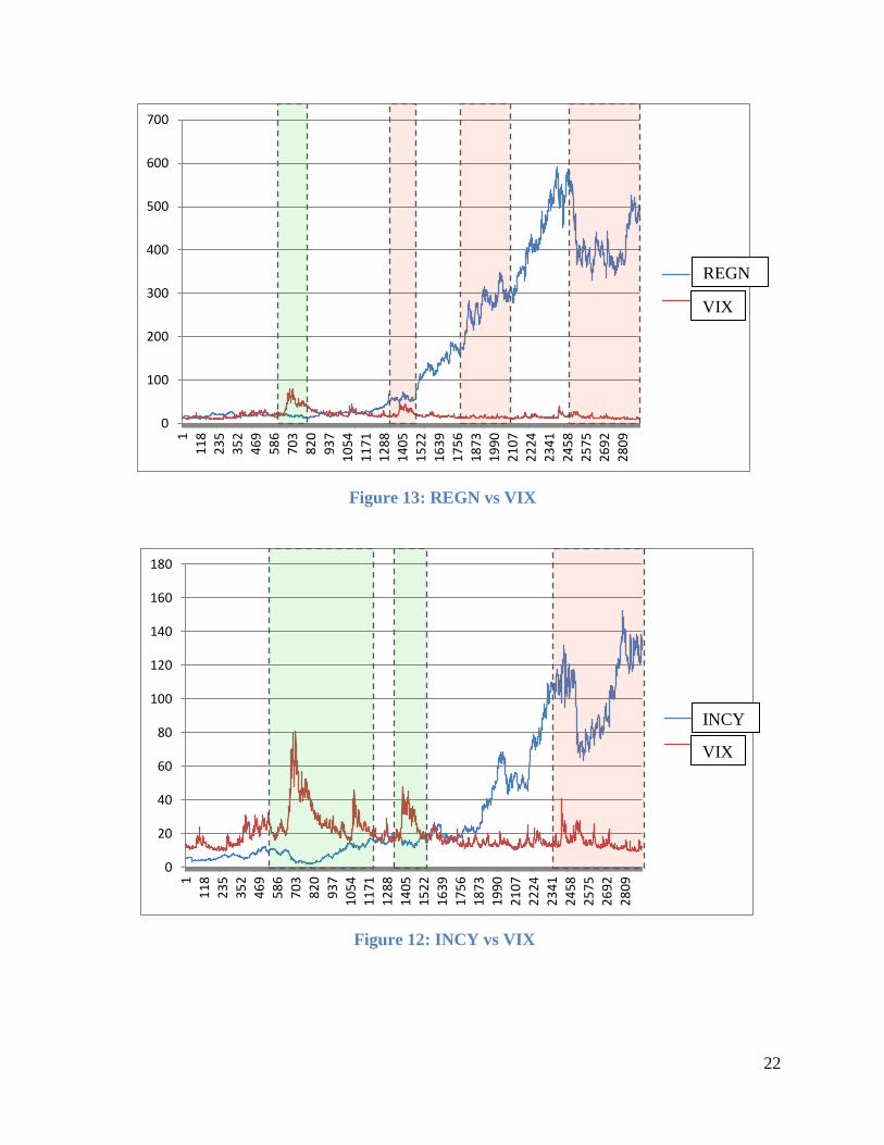
Figure 12: REGN vs VIX ............................................................................................................. 22
Figure 13: INCY vs VIX............................................................................................................... 22
Figure 14: VRTX vs VIX ............................................................................................................. 23
Figure 15: AZN vs VIX ................................................................................................................ 23
Figure 16: Trading Program Interface .......................................................................................... 29
Figure 17: Simulated Returns of Variable Weighting .................................................................. 30
Figure 18: Methods ....................................................................................................................... 32
Figure 19: Trading Strategy Weights ............................................................................................ 33
Figure 20: Earnings of Simulated Strategies over Historical Period Group A ............................. 34
Figure 21 : Earnings of Simulated Strategies over Historical Period Group B ............................ 34
Figure 22: Three Month Returns Group A ................................................................................... 35
Figure 23: Three Month Returns Group B .................................................................................... 36
5
Introduction
In the early twentieth century Henry Poor was walking down the financial district with
John D. Rockefeller. When asked about the future of Standard Oil stocks, Rockefeller is said to
have replied, “Young man, I think they will fluctuate” (Wall Street Journal, 18 Oct. 1922). While
this quote appears shallow at face value, it is profound in how incredibly applicable it is to global
economies today. Within the stock market, fluctuation is a way of life. Prices waver as a result of
countless influences and it is difficult, especially for the inexperienced, to see the broader
patterns of stock movement. Those who find success in trading are the ones who are able to
exploit this volatility in their favor.
To begin to understand the inherent volatility of the market, it is important to understand
the nature of the traders involved. While automation accounts for a large and growing percentage
of trades, human emotion is still deeply rooted in the system. Greed and fear play a significant
role in stock behavior. This is where the VIX comes in to play as potentially a very special
indicator; a way of capturing some of this human emotion into a simple index.
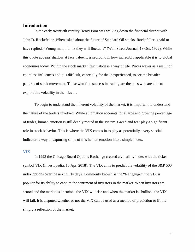
VIX
In 1993 the Chicago Board Options Exchange created a volatility index with the ticker
symbol VIX (Investopedia, 16 Apr. 2018). The VIX aims to predict the volatility of the S&P 500
index options over the next thirty days. Commonly known as the “fear gauge”, the VIX is
popular for its ability to capture the sentiment of investors in the market. When investors are
scared and the market is “bearish” the VIX will rise and when the market is “bullish” the VIX
will fall. It is disputed whether or not the VIX can be used as a method of prediction or if it is
simply a reflection of the market.
6
The VIX is a noteworthy indicator because it gives a representation of far more than just
technical details. Many political, social, and economic events are displayed through investor
sentiment. Theoretically, this gives the VIX an advantage over other technical indicators when it
comes to price prediction. This study attempts to show the potential of the VIX to be used as an
indicator.
Technical Indicators
The significance of technical indicators is a heavily disputed topic by new and
experienced traders alike. While some see them as shortcuts to success, others question just how
well they can distill the intricacies of the market in their basic calculation. A large part of their
criticism comes from the reality that they are not absolute. Specifically, they offer a suggestion
of what is more likely to happen, but offer no guarantee. Because of this, it is important to
recognize that indicators are only as valuable as their user’s understanding of them.
Efficient Market Hypothesis
Developing on this idea, some speculate that the market itself is impossible to beat.
Theorized in the 1960’s by Eugene Fama, the Efficient Market Hypothesis (EMH) suggests that
all of the determinative information, which could potentially be used for prediction, is already
built into the current share price. As a result, technical analysis and exploitation of a stock is
useless. There are three variations of the EMH known as “weak”, “semi-strong”, and “strong”
which increase the extent of the theory (Maverick, 26 Mar. 2015). In the “weak” variation, stock
price is a manifestation of all historical data and, subsequently, technical analysis yields no
predictive information. The “semi-strong” variation adds that any form of fundamental analysis
from public knowledge is also included in the market, making only insider information
7
significant. Finally the “strong” variation includes insider information in the system, making it
impossible to for investors to achieve anything other than normal market returns (Maverick, 26
Mar. 2015). While many agree with the concept of the EMH, it is disputed how well the theory
performs in practice. This study recognizes the existence of some form of the EMH but aims to
disprove its absolute nature.
Ultimately, the goal of this study is to identify the relationships that stocks have with the
VIX and to develop a successful trading strategy around this information. In order to begin to
tackle this problem, a historical analysis of stock data must be performed.
Sample Stocks
The time period being used for the historical analysis begins on 2/6/2006 and ends on
9/8/2017. This data set of 2918 days was chosen because it contains enough points to be
statistically significant and it also contains the entry, crash, and recovery of the 2008 housing
bubble. The stocks that have been chosen to be examined focus in on the biotech and
pharmaceutical sectors of the market in particular. Both individual stocks as well as Exchange
Traded Funds (ETF) were selected to give adequate coverage of the market.
Beta
Calculated through regression analysis, beta gives an indication of a stocks volatility
compared to the market. A beta value greater or less than 1 demonstrates that the stock is more
or less volatile than the market, respectively. When trading, beta is a helpful statistic to consider
because it provides some insight on the risk of an investment. In this study, beta provides a
general indication of the stock’s behavior before doing any technical analysis. Stocks with a
higher beta have higher movement and are potentially more exploitable with trading strategies.
8
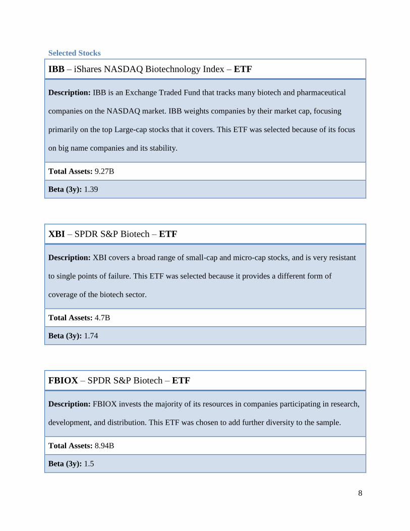
Selected Stocks
IBB – iShares NASDAQ Biotechnology Index – ETF
Description: IBB is an Exchange Traded Fund that tracks many biotech and pharmaceutical
companies on the NASDAQ market. IBB weights companies by their market cap, focusing
primarily on the top Large-cap stocks that it covers. This ETF was selected because of its focus
on big name companies and its stability.
Total Assets: 9.27B
Beta (3y): 1.39
XBI – SPDR S&P Biotech – ETF
Description: XBI covers a broad range of small-cap and micro-cap stocks, and is very resistant
to single points of failure. This ETF was selected because it provides a different form of
coverage of the biotech sector.
Total Assets: 4.7B
Beta (3y): 1.74
FBIOX – SPDR S&P Biotech – ETF
Description: FBIOX invests the majority of its resources in companies participating in research,
development, and distribution. This ETF was chosen to add further diversity to the sample.
Total Assets: 8.94B
Beta (3y): 1.5
9
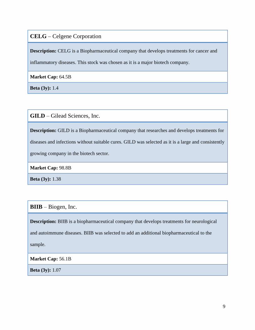
CELG – Celgene Corporation
Description: CELG is a Biopharmaceutical company that develops treatments for cancer and
inflammatory diseases. This stock was chosen as it is a major biotech company.
Market Cap: 64.5B
Beta (3y): 1.4
GILD – Gilead Sciences, Inc.
Description: GILD is a Biopharmaceutical company that researches and develops treatments for
diseases and infections without suitable cures. GILD was selected as it is a large and consistently
growing company in the biotech sector.
Market Cap: 98.8B
Beta (3y): 1.38
BIIB – Biogen, Inc.
Description: BIIB is a biopharmaceutical company that develops treatments for neurological
and autoimmune diseases. BIIB was selected to add an additional biopharmaceutical to the
sample.
Market Cap: 56.1B
Beta (3y): 1.07
10
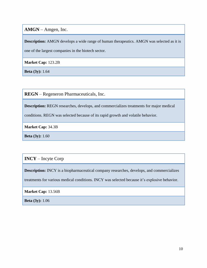
AMGN – Amgen, Inc.
Description: AMGN develops a wide range of human therapeutics. AMGN was selected as it is
one of the largest companies in the biotech sector.
Market Cap: 123.2B
Beta (3y): 1.64
REGN – Regeneron Pharmaceuticals, Inc.
Description: REGN researches, develops, and commercializes treatments for major medical
conditions. REGN was selected because of its rapid growth and volatile behavior.
Market Cap: 34.3B
Beta (3y): 1.60
INCY – Incyte Corp
Description: INCY is a biopharmaceutical company researches, develops, and commercializes
treatments for various medical conditions. INCY was selected because it’s explosive behavior.
Market Cap: 13.56B
Beta (3y): 1.06
11
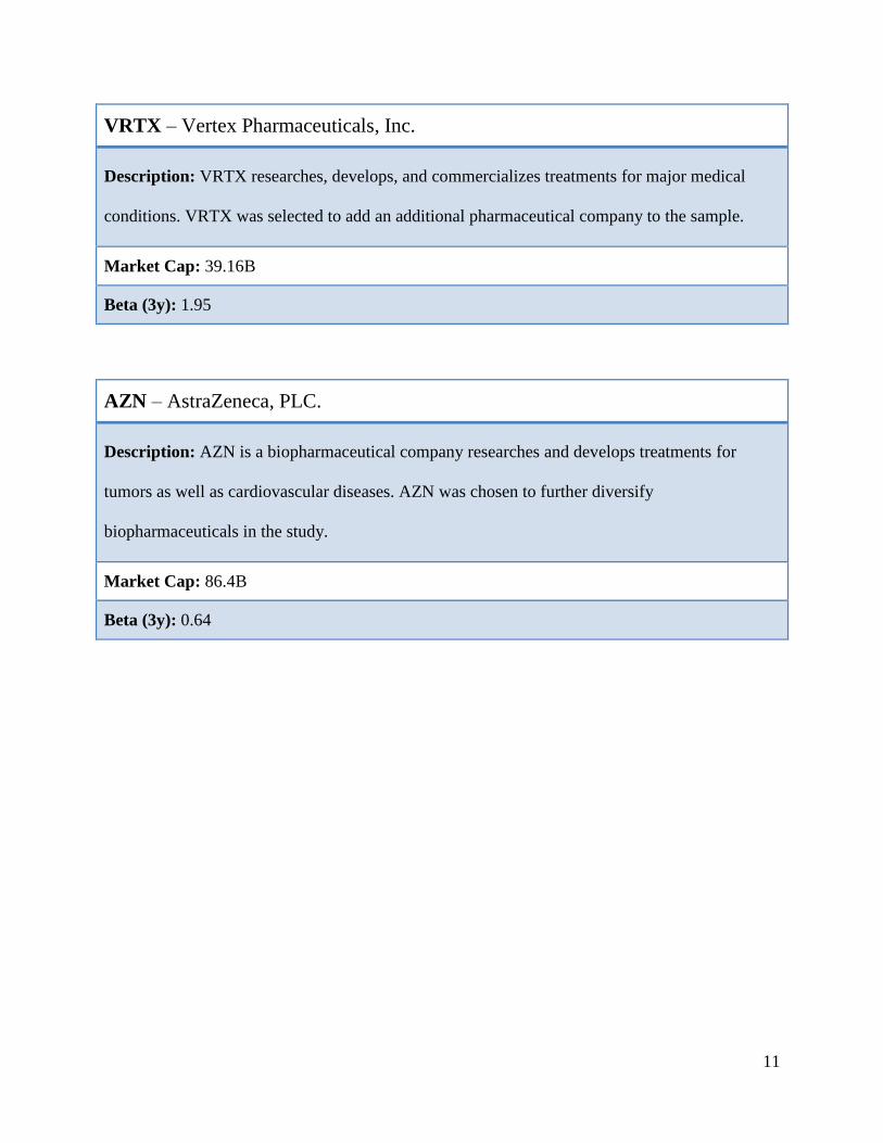
VRTX – Vertex Pharmaceuticals, Inc.
Description: VRTX researches, develops, and commercializes treatments for major medical
conditions. VRTX was selected to add an additional pharmaceutical company to the sample.
Market Cap: 39.16B
Beta (3y): 1.95
AZN – AstraZeneca, PLC.
Description: AZN is a biopharmaceutical company researches and develops treatments for
tumors as well as cardiovascular diseases. AZN was chosen to further diversify
biopharmaceuticals in the study.
Market Cap: 86.4B
Beta (3y): 0.64
12
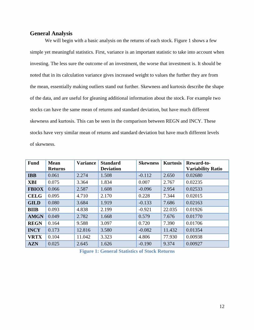
General Analysis
We will begin with a basic analysis on the returns of each stock. Figure 1 shows a few
simple yet meaningful statistics. First, variance is an important statistic to take into account when
investing. The less sure the outcome of an investment, the worse that investment is. It should be
noted that in its calculation variance gives increased weight to values the further they are from
the mean, essentially making outliers stand out further. Skewness and kurtosis describe the shape
of the data, and are useful for gleaning additional information about the stock. For example two
stocks can have the same mean of returns and standard deviation, but have much different
skewness and kurtosis. This can be seen in the comparison between REGN and INCY. These
stocks have very similar mean of returns and standard deviation but have much different levels
of skewness.
Fund Mean
Returns
Variance Standard
Deviation
Skewness Kurtosis Reward-to-
Variability Ratio
IBB 0.061 2.274 1.508 -0.112 2.650 0.02680
XBI 0.075 3.364 1.834 0.007 2.767 0.02235
FBIOX 0.066 2.587 1.608 -0.096 2.954 0.02533
CELG 0.095 4.710 2.170 0.228 7.344 0.02015
GILD 0.080 3.684 1.919 -0.133 7.686 0.02163
BIIB 0.093 4.838 2.199 -0.921 22.035 0.01926
AMGN 0.049 2.782 1.668 0.579 7.676 0.01770
REGN 0.164 9.588 3.097 0.720 7.390 0.01706
INCY 0.173 12.816 3.580 -0.082 11.432 0.01354
VRTX 0.104 11.042 3.323 4.806 77.930 0.00938
AZN 0.025 2.645 1.626 -0.190 9.374 0.00927
Figure 1: General Statistics of Stock Returns

13
From an initial viewing of this data, a few things become apparent. While
pharmaceuticals such as REGN and INCY have the highest mean returns, they also have a higher
volatility making them a higher risk investment. Despite the ETFs IBB and FBIOX having lower
mean returns, they boast the lowest variance resulting in an excellent reward to variability ratio.
Just as would be expected, ETF’s have the highest risk reward ratio, making them strong
investments. While this shows ETF’s as more predictable funds, it does not yet inform us about
how they can be traded.
14
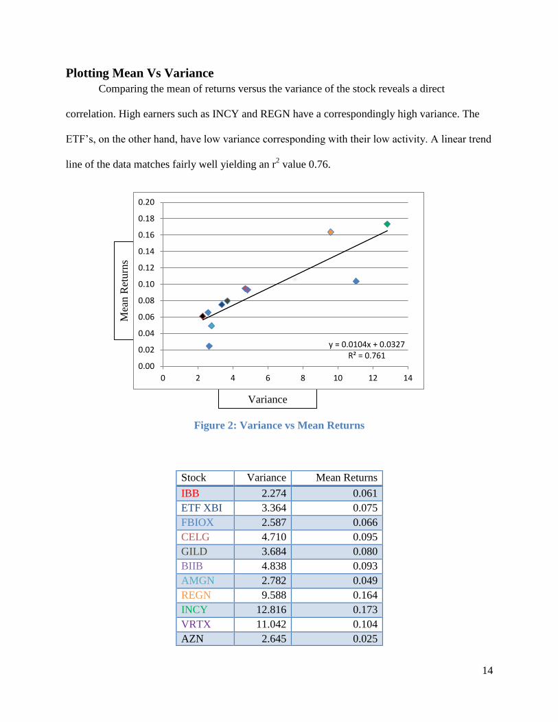
Plotting Mean Vs Variance
Comparing the mean of returns versus the variance of the stock reveals a direct
correlation. High earners such as INCY and REGN have a correspondingly high variance. The
ETF’s, on the other hand, have low variance corresponding with their low activity. A linear trend
line of the data matches fairly well yielding an r2 value 0.76.
Figure 2: Variance vs Mean Returns
Stock Variance Mean Returns
IBB 2.274 0.061
ETF XBI 3.364 0.075
FBIOX 2.587 0.066
CELG 4.710 0.095
GILD 3.684 0.080
BIIB 4.838 0.093
AMGN 2.782 0.049
REGN 9.588 0.164
INCY 12.816 0.173
VRTX 11.042 0.104
AZN 2.645 0.025
Varianc
e
Variance
Mea
n R
eturn
s
y = 0.0104x + 0.0327 R² = 0.761
0.00
0.02
0.04
0.06
0.08
0.10
0.12
0.14
0.16
0.18
0.20
0 2 4 6 8 10 12 14
Mea
n R
eturn
s
15
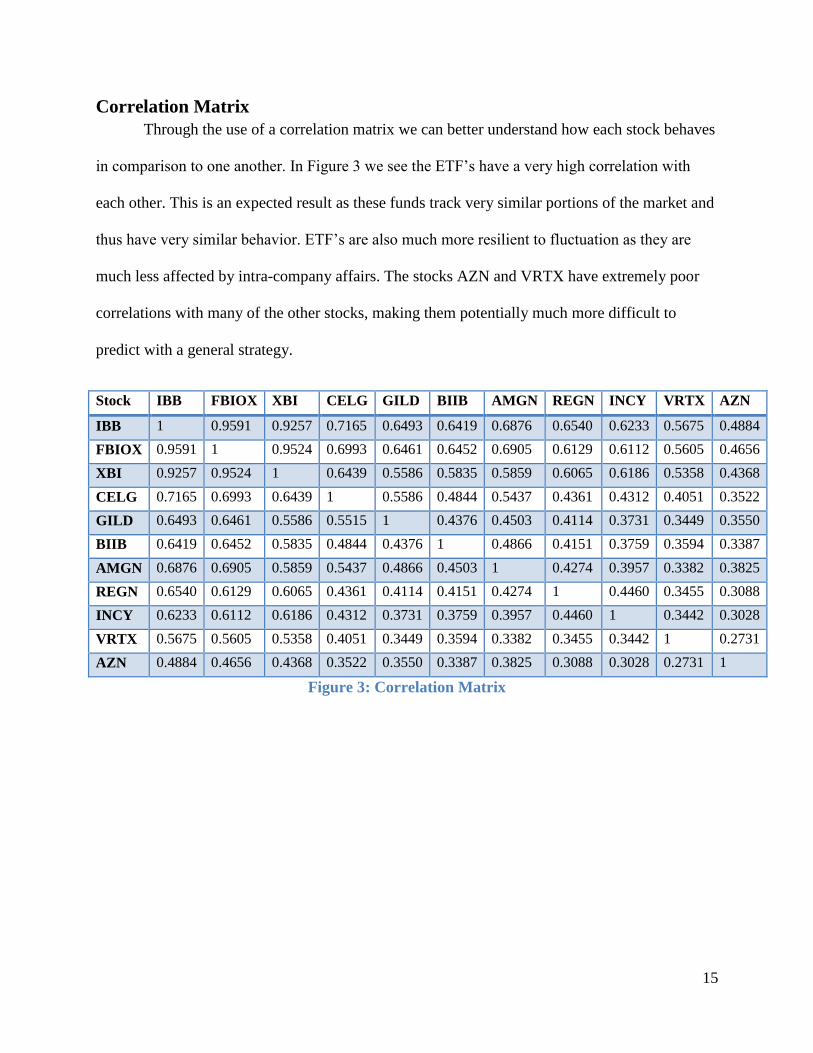
Correlation Matrix
Through the use of a correlation matrix we can better understand how each stock behaves
in comparison to one another. In Figure 3 we see the ETF’s have a very high correlation with
each other. This is an expected result as these funds track very similar portions of the market and
thus have very similar behavior. ETF’s are also much more resilient to fluctuation as they are
much less affected by intra-company affairs. The stocks AZN and VRTX have extremely poor
correlations with many of the other stocks, making them potentially much more difficult to
predict with a general strategy.
Stock IBB FBIOX XBI CELG GILD BIIB AMGN REGN INCY VRTX AZN
IBB 1 0.9591 0.9257 0.7165 0.6493 0.6419 0.6876 0.6540 0.6233 0.5675 0.4884
FBIOX 0.9591 1 0.9524 0.6993 0.6461 0.6452 0.6905 0.6129 0.6112 0.5605 0.4656
XBI 0.9257 0.9524 1 0.6439 0.5586 0.5835 0.5859 0.6065 0.6186 0.5358 0.4368
CELG 0.7165 0.6993 0.6439 1 0.5586 0.4844 0.5437 0.4361 0.4312 0.4051 0.3522
GILD 0.6493 0.6461 0.5586 0.5515 1 0.4376 0.4503 0.4114 0.3731 0.3449 0.3550
BIIB 0.6419 0.6452 0.5835 0.4844 0.4376 1 0.4866 0.4151 0.3759 0.3594 0.3387
AMGN 0.6876 0.6905 0.5859 0.5437 0.4866 0.4503 1 0.4274 0.3957 0.3382 0.3825
REGN 0.6540 0.6129 0.6065 0.4361 0.4114 0.4151 0.4274 1 0.4460 0.3455 0.3088
INCY 0.6233 0.6112 0.6186 0.4312 0.3731 0.3759 0.3957 0.4460 1 0.3442 0.3028
VRTX 0.5675 0.5605 0.5358 0.4051 0.3449 0.3594 0.3382 0.3455 0.3442 1 0.2731
AZN 0.4884 0.4656 0.4368 0.3522 0.3550 0.3387 0.3825 0.3088 0.3028 0.2731 1
Figure 3: Correlation Matrix
16
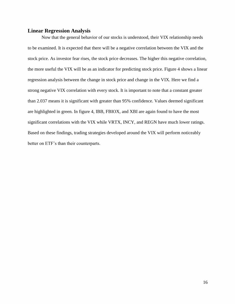
Linear Regression Analysis
Now that the general behavior of our stocks is understood, their VIX relationship needs
to be examined. It is expected that there will be a negative correlation between the VIX and the
stock price. As investor fear rises, the stock price decreases. The higher this negative correlation,
the more useful the VIX will be as an indicator for predicting stock price. Figure 4 shows a linear
regression analysis between the change in stock price and change in the VIX. Here we find a
strong negative VIX correlation with every stock. It is important to note that a constant greater
than 2.037 means it is significant with greater than 95% confidence. Values deemed significant
are highlighted in green. In figure 4, IBB, FBIOX, and XBI are again found to have the most
significant correlations with the VIX while VRTX, INCY, and REGN have much lower ratings.
Based on these findings, trading strategies developed around the VIX will perform noticeably
better on ETF’s than their counterparts.
17
FUND Constant Δ VIX
IBB 0.0944 -0.1220
(4.30) (-42.42)
FBIOX 0.1000 -0.1258
(4.18) (-40.20)
XBI 0.1121 -0.1347
(3.98) (-36.57)
CELG 0.1303 -0.1293
(3.64) (-27.56)
GILD 0.1104 -0.1122
(3.47) (-26.93)
BIIB 0.1256 -0.1185
(3.38) (-24.37)
AMGN 0.0764 -0.0992
(2.78) (-27.51)
REGN 0.2066 -0.1569
(3.91) (-22.64)
INCY 0.2240 -0.1844
(3.67) (-23.10)
VRTX 0.1435 -0.1457
(2.47) (-19.18)
AZN 0.0507 -0.0957
(1.88) (-27.14)
Figure 4: Regression Statistics of Returns vs VIX
18
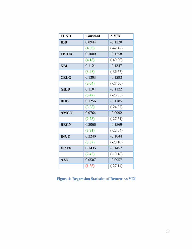
Plotting Stocks vs the VIX
Plotting stocks against the VIX give a good visual indication of the relationship. It can
clearly be seen when the VIX successfully reflects the behavior of a stock and when it does not.
Often the stock and the VIX act as reflections of each other. However, there are also some
situations where the stock fluctuations are completely unnoticed in the VIX and vice-versa. In
the Figures below, behavior that suggests strong correlation is highlighted in green, and behavior
that suggests poor correlation is highlighted in red.
Figure 5: IBB vs VIX
0
50
100
150
200
250
300
350
400
450
1
11
8
23
53
52
46
95
86
70
38
20
93
7
10
54
11
71
12
88
14
05
15
22
16
39
17
56
18
73
19
90
21
07
22
24
23
41
24
58
25
75
26
92
28
09
Series1
Series2
IBB
VIX
19
Figure 6: FBIOX vs VIX
Figure 7: XBI vs VIX
0
50
100
150
200
250
300
1
11
8
23
5
35
2
46
9
58
6
70
3
82
0
93
7
10
54
11
71
12
88
14
05
15
22
16
39
17
56
18
73
19
90
21
07
22
24
23
41
24
58
25
75
26
92
28
09
Series1
Series2
0
10
20
30
40
50
60
70
80
90
100
1
11
8
23
5
35
2
46
9
58
6
70
3
82
0
93
7
10
54
11
71
12
88
14
05
15
22
16
39
17
56
18
73
19
90
21
07
22
24
23
41
24
58
25
75
26
92
28
09
Series1
Series2
FBIOX
VIX
XBI
VIX
20
Figure 8: CELG VS VIX
Figure 9: GILD vs VIX
0
20
40
60
80
100
120
140
160
1
11
8
23
5
35
2
46
9
58
6
70
3
82
0
93
7
10
54
11
71
12
88
14
05
15
22
16
39
17
56
18
73
19
90
21
07
22
24
23
41
24
58
25
75
26
92
28
09
Series1
Series2
0
20
40
60
80
100
120
140
1
11
8
23
5
35
2
46
9
58
6
70
3
82
0
93
7
10
54
11
71
12
88
14
05
15
22
16
39
17
56
18
73
19
90
21
07
22
24
23
41
24
58
25
75
26
92
28
09
Series1
Series2
CELG
VIX
GILD
VIX
21
Figure 10: BIIB vs VIX
Figure 11: AMGN vs VIX
0
50
100
150
200
250
300
350
400
450
500
1
11
8
23
5
35
2
46
9
58
6
70
3
82
0
93
7
10
54
11
71
12
88
14
05
15
22
16
39
17
56
18
73
19
90
21
07
22
24
23
41
24
58
25
75
26
92
28
09
Series1
Series2
0
20
40
60
80
100
120
140
160
180
200
1
11
8
23
5
35
2
46
9
58
6
70
3
82
0
93
7
10
54
11
71
12
88
14
05
15
22
16
39
17
56
18
73
19
90
21
07
22
24
23
41
24
58
25
75
26
92
28
09
Series1
Series2
BIIB
VIX
AMGN
VIX
22
Figure 13: REGN vs VIX
0
100
200
300
400
500
600
700
1
11
8
23
5
35
2
46
9
58
6
70
3
82
0
93
7
10
54
11
71
12
88
14
05
15
22
16
39
17
56
18
73
19
90
21
07
22
24
23
41
24
58
25
75
26
92
28
09
Series1
Series2
0
20
40
60
80
100
120
140
160
180
1
11
8
23
5
35
2
46
9
58
6
70
3
82
0
93
7
10
54
11
71
12
88
14
05
15
22
16
39
17
56
18
73
19
90
21
07
22
24
23
41
24
58
25
75
26
92
28
09
Series1
Series2
REGN
VIX
INCY
VIX
Figure 12: INCY vs VIX

23
Figure 14: VRTX vs VIX
Figure 15: AZN vs VIX
0
20
40
60
80
100
120
140
160
180
1
11
8
23
5
35
2
46
9
58
6
70
3
82
0
93
7
10
54
11
71
12
88
14
05
15
22
16
39
17
56
18
73
19
90
21
07
22
24
23
41
24
58
25
75
26
92
28
09
Series1
Series2
0
10
20
30
40
50
60
70
80
90
11
14
22
73
40
45
35
66
67
97
92
90
51
01
81
13
11
24
41
35
71
47
01
58
31
69
61
80
91
92
22
03
52
14
82
26
12
37
42
48
72
60
02
71
32
82
6
Series1
Series2
VIX
AZN
VIX
VRTX
24
Creating a Trading Program
Now that we have found these stocks to have a meaningful correlation with the VIX, we
can use this knowledge to develop a strategy for trading. While the VIX inherently contains
some information about investor sentiment on a macro scale, our trading system will not be able
to predict any impactful future events, especially specific to each stock. For example our trading
strategy will have no way of knowing about upcoming financial reports, government legislation,
or new breakthrough cancer drugs. Ultimately, our trading strategy focuses on the technical
aspects of trading rather than the fundamentals.
To create a trading strategy we must define the rules to buy and sell a stock. In order to
improve accuracy, the weights of each rule can be adjusted relative to each other through
simulation. To begin we will define a few somewhat arbitrary rules that can be improved in the
future. The goal here is to establish the problem space and the program will help locate optimal
strategies within the environment. In order to evaluate the VIX trading strategy, additional
trading strategies will be created using other technical indicators. This gives us more contexts to
evaluate the VIX trading strategy.
RSI
The Relative Strength Index (RSI) is a popular technical indicator that describes the
recent performance of a stock and its current momentum. Generally, a value greater than 70
indicates that a stock price is overbought and a value lower than thirty indicates that a stock is
oversold (StockCharts.com, 9 Oct. 2017). While the RSI can lead to false signals, it can be
effective at highlighting trends when used in conjunction with other indicators.
25
Moving Average
The two primary types of moving averages are the Simple Moving Average (SMA) and
the Exponential Moving Average (EMA). Moving averages are basic methods used to reduce
noise in stock data, revealing larger scale trends. EMAs are similar to SMAs in their calculation,
but give heavier weighting to more recent data. This allows them to respond more quickly to
rapid changes and breakouts. Moving averages of different lengths (10 day, 20 day, 60 day) are
used in conjunction with each other to find buy and sell signals. When the indicators cross one
another it represents a potential place to make a trade. In our trading program, SMAs and EMAs
are used for pattern recognition in VIX and stock data.
On Balance Volume
On balance volume (OBV) is a momentum indicator that focuses on volume rather than
price. The theory of OBV is based on the basic idea that large changes in volume without
changes in stock price are a sign of significant future price movement. Its calculation simply
involves adding volume on days where the stock price goes up and subtracting when it goes
down.
26
Trading Rules
The following are the initial VIX trading rules used by all five trading strategies.
Buy If the VIX low is above its 10 day simple moving average
Sell if the VIX high is below its 10 day simple moving average
Buy if the VIX close is more than 10% above its 10 day exponential moving average
Sell if the VIX high is more than 10% below its 10 day exponential moving average
Buy if the VIX close is less than 13
Sell if the VIX close is more than 25
Buy if the VIX has gone up more than 9% in one day
Sell if the VIX has gone down more than 9% in one day
Below are additional indicators used in methods one, two, and three.
Simple Moving Average
Buy if the 5 day SMA of the stock price crosses above the 10 day SMA
Sell if the 5 day SMA of the stock price crosses below the 10 day SMA
RSI Rules
Sell if the RSI is above 65
Buy if the RSI is below 35
On Balance Volume Rules
Buy If the slope of the stocks 10 day SMA is moving upwards more than 7% and the
slope of the 10 day SMA of the on balance volume is within 5% of the stocks slope
Sell If the slope of the stocks 10 day SMA is moving upwards more than 7% and the
slope of the 10 day SMA of the on balance volume is not within 5% of the stocks slope

27
Sell If the slope of the stocks 10 day SMA is moving downwards more than 7% and the
slope of the 10 day SMA of the on balance volume is within 5% of the stocks slope
Buy If the slope of the stocks 10 day SMA is moving upwards more than 7% and the
slope of the 10 day SMA of the on balance volume is not within 5% of the stocks slope
Sell if the difference between the two slopes is greater than 5% and the OBV is moving
downwards
Buy if the difference between the two slopes is greater than 5% and the OBV is moving
upwards
28
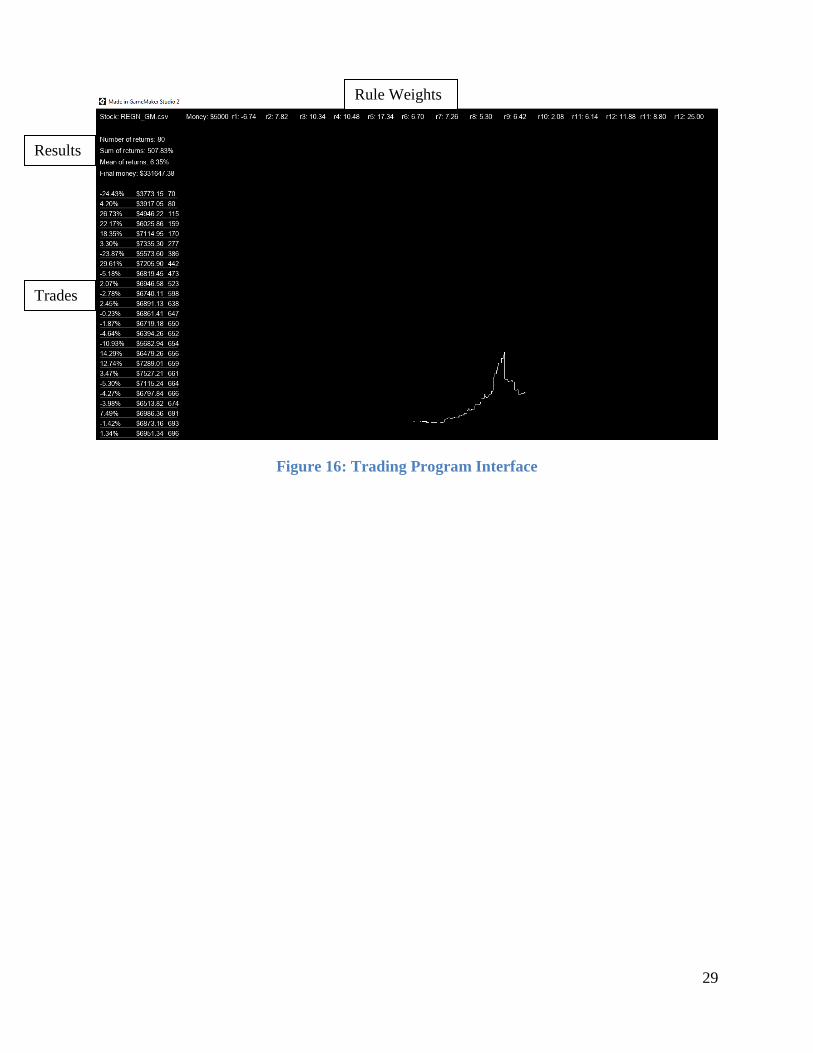
Trading Program
The program developed is able to import the data for each stock and simulate trading
based on that data. The data is first processed in Excel to calculate the indicators and is then
imported into the program. Built into the program is a $7.00 commission fee on each trade. This
discourages the program from optimizing for trading strategies with many hundreds of trades. By
default the program starts with $5000.00 of currency.
Weighting
The rules were implemented as seen above but a variable weighting system was
implemented alongside to change the impact of each rule at runtime. When the rules are met, the
given weight is added to the score that will determine to buy or sell. Because of this variable
weighting system, weights can be set to negative values. This gives the program an extremely
wide range of options when optimizing. Some rules may turn out to work in the opposite
direction than we intended. The program is setup with 14 different weights. Unfortunately, due
to the limits of processing power, every combination of these weights cannot be tested. The user
must instead manually adjust one variable at a time.
29
Figure 16: Trading Program Interface
Trades
Rule Weights
Results
30
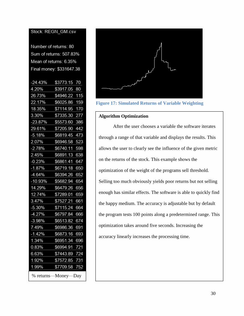
% returns—Money—Day
Algorithm Optimization
After the user chooses a variable the software iterates
through a range of that variable and displays the results. This
allows the user to clearly see the influence of the given metric
on the returns of the stock. This example shows the
optimization of the weight of the programs sell threshold.
Selling too much obviously yields poor returns but not selling
enough has similar effects. The software is able to quickly find
the happy medium. The accuracy is adjustable but by default
the program tests 100 points along a predetermined range. This
optimization takes around five seconds. Increasing the
accuracy linearly increases the processing time.
Figure 17: Simulated Returns of Variable Weighting
31
Optimizing for Individual Stocks vs All Stocks
Different stocks often have very different behavior from one another. This is a
culmination of financial reports, insider trading, global market activity, legislation, etc. As can be
seen in figure 4, different stocks also have largely varying correlations with the VIX. The goal is
to take advantage of the commonalties in stock movements to create a globally successful
strategy.
The program is able to go through historical data and test the weighting of a given rule to
find the value that produces maximum income. If we attempt to optimize for GILD for example,
the program will only take GILD’s behavior into account when optimizing the variable. This can
be problematic when optimizing for two stocks that have noticeably different behavior. Take
VRTX and AZN from figure 3 for example. As we can see from the correlation matrix, the
stocks have a correlation of 0.2730. Obviously, an optimal strategy for VRTX would look quite
different from an optimal strategy for AZN. This raises a fundamental question. Which method
has more accurate results? Optimizing for unique stocks on an individual basis or developing a
single strategy that has optimal returns over a large variety of sample stocks. Due to scope, all of
the created strategies were one size fits all. Given these conditions, six methods of variable
weighting were developed to find the optimal trading strategy. The weighting that provides the
highest return and lowest variance between stocks is the optimal strategy.
32
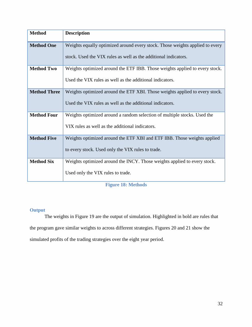
Method Description
Method One Weights equally optimized around every stock. Those weights applied to every
stock. Used the VIX rules as well as the additional indicators.
Method Two Weights optimized around the ETF IBB. Those weights applied to every stock.
Used the VIX rules as well as the additional indicators.
Method Three Weights optimized around the ETF XBI. Those weights applied to every stock.
Used the VIX rules as well as the additional indicators.
Method Four Weights optimized around a random selection of multiple stocks. Used the
VIX rules as well as the additional indicators.
Method Five Weights optimized around the ETF XBI and ETF IBB. Those weights applied
to every stock. Used only the VIX rules to trade.
Method Six Weights optimized around the INCY. Those weights applied to every stock.
Used only the VIX rules to trade.
Figure 18: Methods
Output
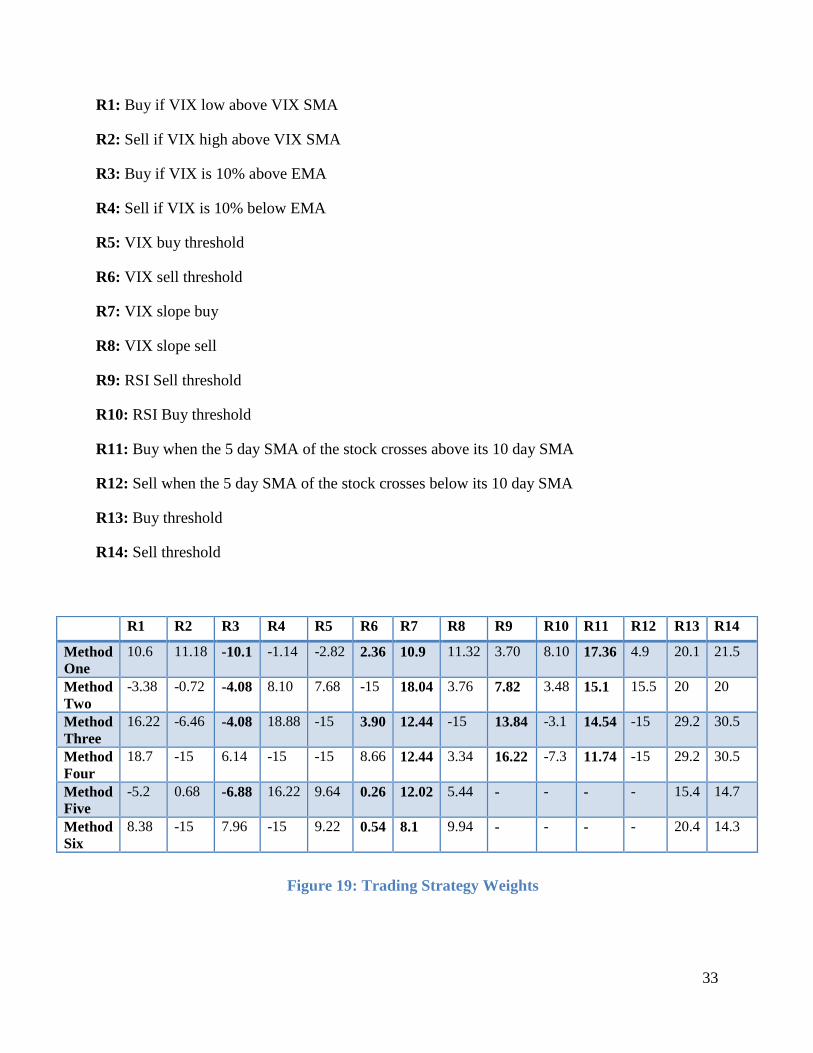
The weights in Figure 19 are the output of simulation. Highlighted in bold are rules that
the program gave similar weights to across different strategies. Figures 20 and 21 show the
simulated profits of the trading strategies over the eight year period.
33
R1: Buy if VIX low above VIX SMA
R2: Sell if VIX high above VIX SMA
R3: Buy if VIX is 10% above EMA
R4: Sell if VIX is 10% below EMA
R5: VIX buy threshold
R6: VIX sell threshold
R7: VIX slope buy
R8: VIX slope sell
R9: RSI Sell threshold
R10: RSI Buy threshold
R11: Buy when the 5 day SMA of the stock crosses above its 10 day SMA
R12: Sell when the 5 day SMA of the stock crosses below its 10 day SMA
R13: Buy threshold
R14: Sell threshold
R1 R2 R3 R4 R5 R6 R7 R8 R9 R10 R11 R12 R13 R14
Method
One
10.6 11.18 -10.1 -1.14 -2.82 2.36 10.9 11.32 3.70 8.10 17.36 4.9 20.1 21.5
Method
Two
-3.38 -0.72 -4.08 8.10 7.68 -15 18.04 3.76 7.82 3.48 15.1 15.5 20 20
Method
Three
16.22 -6.46 -4.08 18.88 -15 3.90 12.44 -15 13.84 -3.1 14.54 -15 29.2 30.5
Method
Four
18.7 -15 6.14 -15 -15 8.66 12.44 3.34 16.22 -7.3 11.74 -15 29.2 30.5
Method
Five
-5.2 0.68 -6.88 16.22 9.64 0.26 12.02 5.44 - - - - 15.4 14.7
Method
Six
8.38 -15 7.96 -15 9.22 0.54 8.1 9.94 - - - - 20.4 14.3
Figure 19: Trading Strategy Weights
34
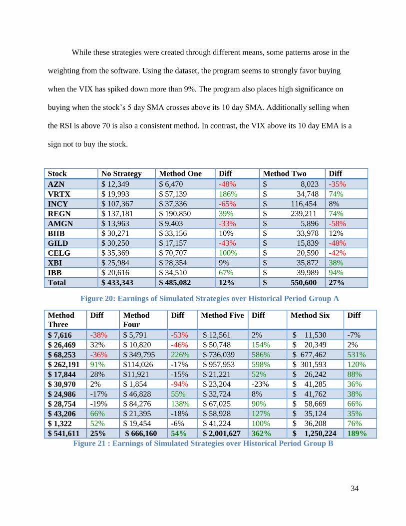
While these strategies were created through different means, some patterns arose in the
weighting from the software. Using the dataset, the program seems to strongly favor buying
when the VIX has spiked down more than 9%. The program also places high significance on
buying when the stock’s 5 day SMA crosses above its 10 day SMA. Additionally selling when
the RSI is above 70 is also a consistent method. In contrast, the VIX above its 10 day EMA is a
sign not to buy the stock.
Method
Three
Diff Method
Four
Diff Method Five Diff Method Six Diff
$ 7,616 -38% $ 5,791 -53% $ 12,561 2% $ 11,530 -7%
$ 26,469 32% $ 10,820 -46% $ 50,748 154% $ 20,349 2%
$ 68,253 -36% $ 349,795 226% $ 736,039 586% $ 677,462 531%
$ 262,191 91% $114,026 -17% $ 957,953 598% $ 301,593 120%
$ 17,844 28% $11,921 -15% $ 21,221 52% $ 26,242 88%
$ 30,970 2% $ 1,854 -94% $ 23,204 -23% $ 41,285 36%
$ 24,986 -17% $ 46,828 55% $ 32,724 8% $ 41,762 38%
$ 28,754 -19% $ 84,276 138% $ 67,025 90% $ 58,669 66%
$ 43,206 66% $ 21,395 -18% $ 58,928 127% $ 35,124 35%
$ 1,322 52% $ 19,454 -6% $ 41,224 100% $ 36,208 76%
$ 541,611 25% $ 666,160 54% $ 2,001,627 362% $ 1,250,224 189%
Figure 21 : Earnings of Simulated Strategies over Historical Period Group B
Stock No Strategy Method One Diff Method Two Diff
AZN $ 12,349 $ 6,470 -48% $ 8,023 -35%
VRTX $ 19,993 $ 57,139 186% $ 34,748 74%
INCY $ 107,367 $ 37,336 -65% $ 116,454 8%
REGN $ 137,181 $ 190,850 39% $ 239,211 74%
AMGN $ 13,963 $ 9,403 -33% $ 5,896 -58%
BIIB $ 30,271 $ 33,156 10% $ 33,978 12%
GILD $ 30,250 $ 17,157 -43% $ 15,839 -48%
CELG $ 35,369 $ 70,707 100% $ 20,590 -42%
XBI $ 25,984 $ 28,354 9% $ 35,872 38%
IBB $ 20,616 $ 34,510 67% $ 39,989 94%
Total $ 433,343 $ 485,082 12% $ 550,600 27%
Figure 20: Earnings of Simulated Strategies over Historical Period Group A
35
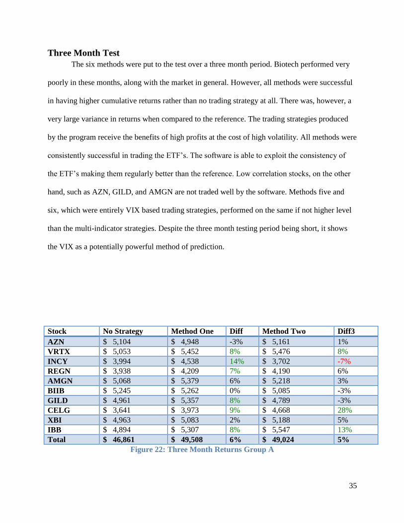
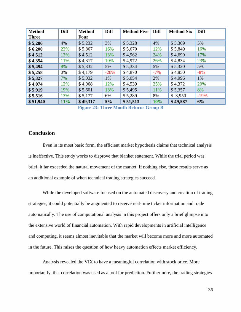
Three Month Test
The six methods were put to the test over a three month period. Biotech performed very
poorly in these months, along with the market in general. However, all methods were successful
in having higher cumulative returns rather than no trading strategy at all. There was, however, a
very large variance in returns when compared to the reference. The trading strategies produced
by the program receive the benefits of high profits at the cost of high volatility. All methods were
consistently successful in trading the ETF’s. The software is able to exploit the consistency of
the ETF’s making them regularly better than the reference. Low correlation stocks, on the other
hand, such as AZN, GILD, and AMGN are not traded well by the software. Methods five and
six, which were entirely VIX based trading strategies, performed on the same if not higher level
than the multi-indicator strategies. Despite the three month testing period being short, it shows
the VIX as a potentially powerful method of prediction.
Stock No Strategy Method One Diff Method Two Diff3
AZN $ 5,104 $ 4,948 -3% $ 5,161 1%
VRTX $ 5,053 $ 5,452 8% $ 5,476 8%
INCY $ 3,994 $ 4,538 14% $ 3,702 -7%
REGN $ 3,938 $ 4,209 7% $ 4,190 6%
AMGN $ 5,068 $ 5,379 6% $ 5,218 3%
BIIB $ 5,245 $ 5,262 0% $ 5,085 -3%
GILD $ 4,961 $ 5,357 8% $ 4,789 -3%
CELG $ 3,641 $ 3,973 9% $ 4,668 28%
XBI $ 4,963 $ 5,083 2% $ 5,188 5%
IBB $ 4,894 $ 5,307 8% $ 5,547 13%
Total $ 46,861 $ 49,508 6% $ 49,024 5%
Figure 22: Three Month Returns Group A
36
Method
Three
Diff Method
Four
Diff Method Five Diff Method Six Diff
$ 5,286 4% $ 5,232 3% $ 5,328 4% $ 5,369 5%
$ 6,200 23% $ 5,867 16% $ 5,670 12% $ 5,849 16%
$ 4,512 13% $ 4,512 13% $ 4,962 24% $ 4,690 17%
$ 4,354 11% $ 4,317 10% $ 4,972 26% $ 4,834 23%
$ 5,494 8% $ 5,332 5% $ 5,334 5% $ 5,320 5%
$ 5,258 0% $ 4,179 -20% $ 4,870 -7% $ 4,850 -8%
$ 5,327 7% $ 5,032 1% $ 5,054 2% $ 4,996 1%
$ 4,074 12% $ 4,068 12% $ 4,539 25% $ 4,372 20%
$ 5,919 19% $ 5,601 13% $ 5,495 11% $ 5,357 8%
$ 5,516 13% $ 5,177 6% $ 5,289 8% $ 3,950 -19%
$ 51,940 11% $ 49,317 5% $ 51,513 10% $ 49,587 6%
Figure 23: Three Month Returns Group B
Conclusion
Even in its most basic form, the efficient market hypothesis claims that technical analysis
is ineffective. This study works to disprove that blanket statement. While the trial period was
brief, it far exceeded the natural movement of the market. If nothing else, these results serve as
an additional example of when technical trading strategies succeed.
While the developed software focused on the automated discovery and creation of trading
strategies, it could potentially be augmented to receive real-time ticker information and trade
automatically. The use of computational analysis in this project offers only a brief glimpse into
the extensive world of financial automation. With rapid developments in artificial intelligence
and computing, it seems almost inevitable that the market will become more and more automated
in the future. This raises the question of how heavy automation effects market efficiency.
Analysis revealed the VIX to have a meaningful correlation with stock price. More
importantly, that correlation was used as a tool for prediction. Furthermore, the trading strategies
37
based entirely off of the VIX outperformed trading strategies with other traditional indicators.
The VIX is not merely a reflection of the market but is a collection of information that can be
exploited.
Work Cited
“Efficient Market Hypothesis (EMH).” Investopedia, Investopedia, 28 Sept. 2016,
www.investopedia.com/terms/e/efficientmarkethypothesis.asp.
“Relative Strength Index (RSI).” StockCharts.com, 9 Oct. 2017,
www.stockcharts.com/school/doku.php?id=chart_school%3Atechnical_indicators%3Arelative_s
trength_index_rsi.
Maverick, J.B. “What Are the Differences between Weak, Strong and Semi-Strong Versions of
the Efficient Market Hypothesis?” Investopedia, Investopedia, 26 Mar. 2015,
www.investopedia.com/ask/answers/032615/what-are-differences-between-weak-strong-and-
semistrong-versions-efficient-market-hypothesis.asp.
1922 October 18, Wall Street Journal, What of the Market?, Quote Page 2, Column 5, New
York. (ProQuest)
“VIX - CBOE Volatility Index.” Investopedia, Investopedia, 16 Apr. 2018,
www.investopedia.com/terms/v/vix.asp
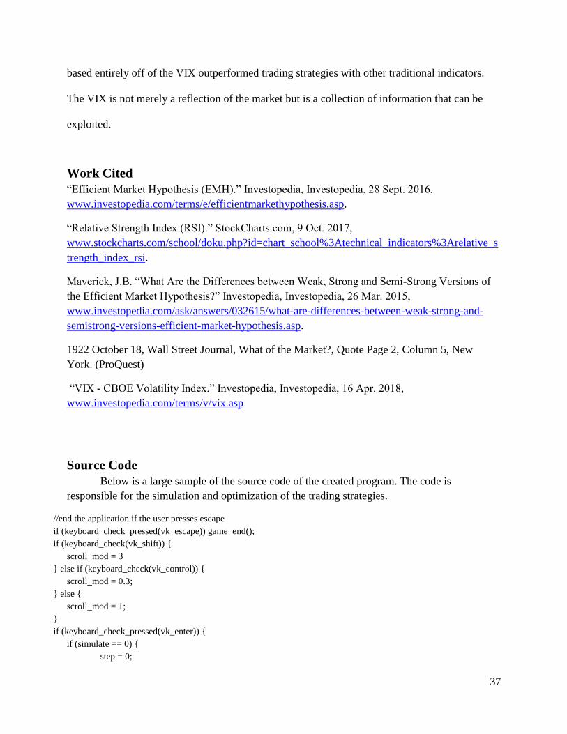
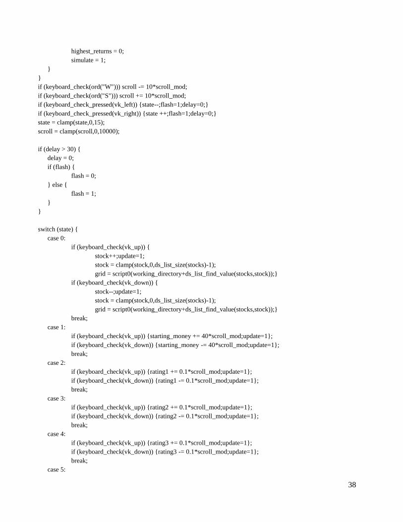
Source Code
Below is a large sample of the source code of the created program. The code is
responsible for the simulation and optimization of the trading strategies.
//end the application if the user presses escape
if (keyboard_check_pressed(vk_escape)) game_end();
if (keyboard_check(vk_shift)) {
scroll_mod = 3
} else if (keyboard_check(vk_control)) {
scroll_mod = 0.3;
} else {
scroll_mod = 1;
}
if (keyboard_check_pressed(vk_enter)) {
if (simulate == 0) {
step = 0;
38
highest_returns = 0;
simulate = 1;
}
}
if (keyboard_check(ord("W"))) scroll -= 10*scroll_mod;
if (keyboard_check(ord("S"))) scroll += 10*scroll_mod;
if (keyboard_check_pressed(vk_left)) {state--;flash=1;delay=0;}
if (keyboard_check_pressed(vk_right)) {state ++;flash=1;delay=0;}
state = clamp(state,0,15);
scroll = clamp(scroll,0,10000);
if (delay > 30) {
delay = 0;
if (flash) {
flash = 0;
} else {
flash = 1;
}
}
switch (state) {
case 0:
if (keyboard_check(vk_up)) {
stock++;update=1;
stock = clamp(stock,0,ds_list_size(stocks)-1);
grid = script0(working_directory+ds_list_find_value(stocks,stock));}
if (keyboard_check(vk_down)) {
stock--;update=1;
stock = clamp(stock,0,ds_list_size(stocks)-1);
grid = script0(working_directory+ds_list_find_value(stocks,stock));}
break;
case 1:
if (keyboard_check(vk_up)) {starting_money += 40*scroll_mod;update=1};
if (keyboard_check(vk_down)) {starting_money -= 40*scroll_mod;update=1};
break;
case 2:
if (keyboard_check(vk_up)) {rating1 += 0.1*scroll_mod;update=1};
if (keyboard_check(vk_down)) {rating1 -= 0.1*scroll_mod;update=1};
break;
case 3:
if (keyboard_check(vk_up)) {rating2 += 0.1*scroll_mod;update=1};
if (keyboard_check(vk_down)) {rating2 -= 0.1*scroll_mod;update=1};
break;
case 4:
if (keyboard_check(vk_up)) {rating3 += 0.1*scroll_mod;update=1};
if (keyboard_check(vk_down)) {rating3 -= 0.1*scroll_mod;update=1};
break;
case 5:
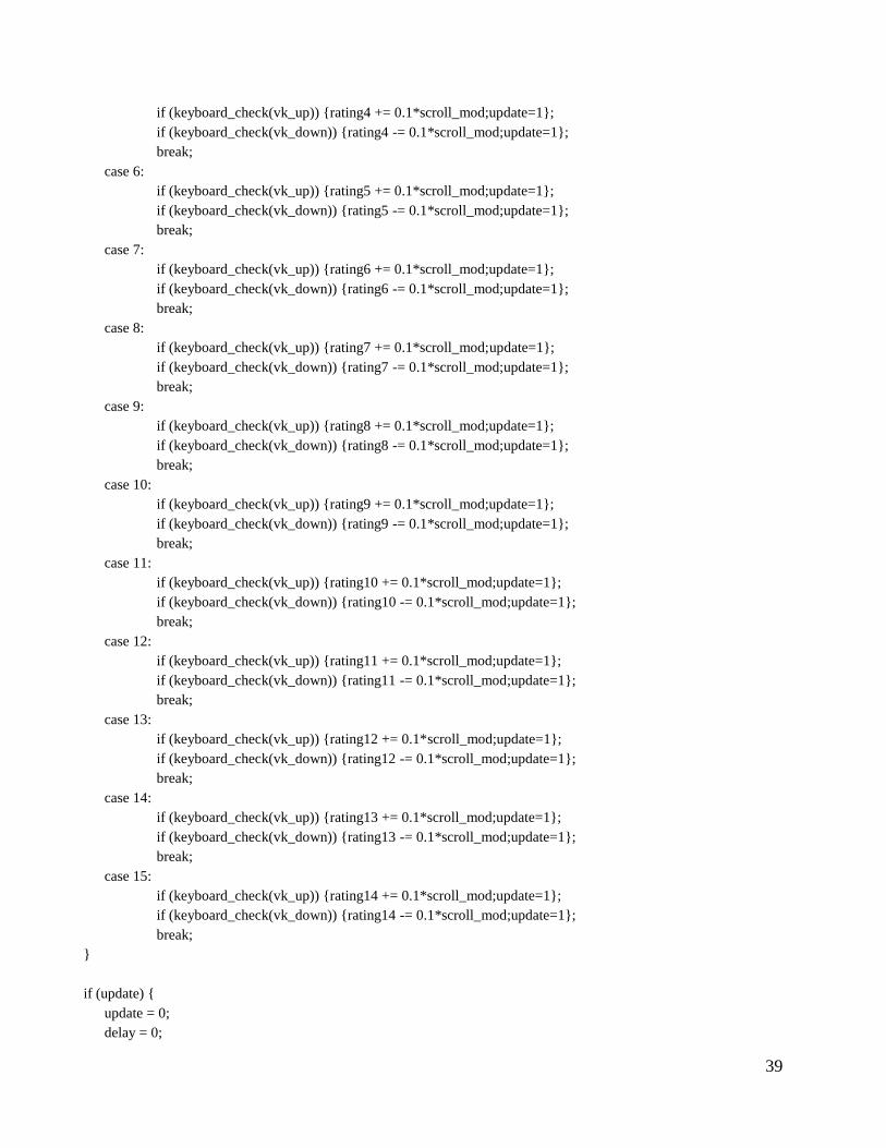
39
if (keyboard_check(vk_up)) {rating4 += 0.1*scroll_mod;update=1};
if (keyboard_check(vk_down)) {rating4 -= 0.1*scroll_mod;update=1};
break;
case 6:
if (keyboard_check(vk_up)) {rating5 += 0.1*scroll_mod;update=1};
if (keyboard_check(vk_down)) {rating5 -= 0.1*scroll_mod;update=1};
break;
case 7:
if (keyboard_check(vk_up)) {rating6 += 0.1*scroll_mod;update=1};
if (keyboard_check(vk_down)) {rating6 -= 0.1*scroll_mod;update=1};
break;
case 8:
if (keyboard_check(vk_up)) {rating7 += 0.1*scroll_mod;update=1};
if (keyboard_check(vk_down)) {rating7 -= 0.1*scroll_mod;update=1};
break;
case 9:
if (keyboard_check(vk_up)) {rating8 += 0.1*scroll_mod;update=1};
if (keyboard_check(vk_down)) {rating8 -= 0.1*scroll_mod;update=1};
break;
case 10:
if (keyboard_check(vk_up)) {rating9 += 0.1*scroll_mod;update=1};
if (keyboard_check(vk_down)) {rating9 -= 0.1*scroll_mod;update=1};
break;
case 11:
if (keyboard_check(vk_up)) {rating10 += 0.1*scroll_mod;update=1};
if (keyboard_check(vk_down)) {rating10 -= 0.1*scroll_mod;update=1};
break;
case 12:
if (keyboard_check(vk_up)) {rating11 += 0.1*scroll_mod;update=1};
if (keyboard_check(vk_down)) {rating11 -= 0.1*scroll_mod;update=1};
break;
case 13:
if (keyboard_check(vk_up)) {rating12 += 0.1*scroll_mod;update=1};
if (keyboard_check(vk_down)) {rating12 -= 0.1*scroll_mod;update=1};
break;
case 14:
if (keyboard_check(vk_up)) {rating13 += 0.1*scroll_mod;update=1};
if (keyboard_check(vk_down)) {rating13 -= 0.1*scroll_mod;update=1};
break;
case 15:
if (keyboard_check(vk_up)) {rating14 += 0.1*scroll_mod;update=1};
if (keyboard_check(vk_down)) {rating14 -= 0.1*scroll_mod;update=1};
break;
}
if (update) {
update = 0;
delay = 0;
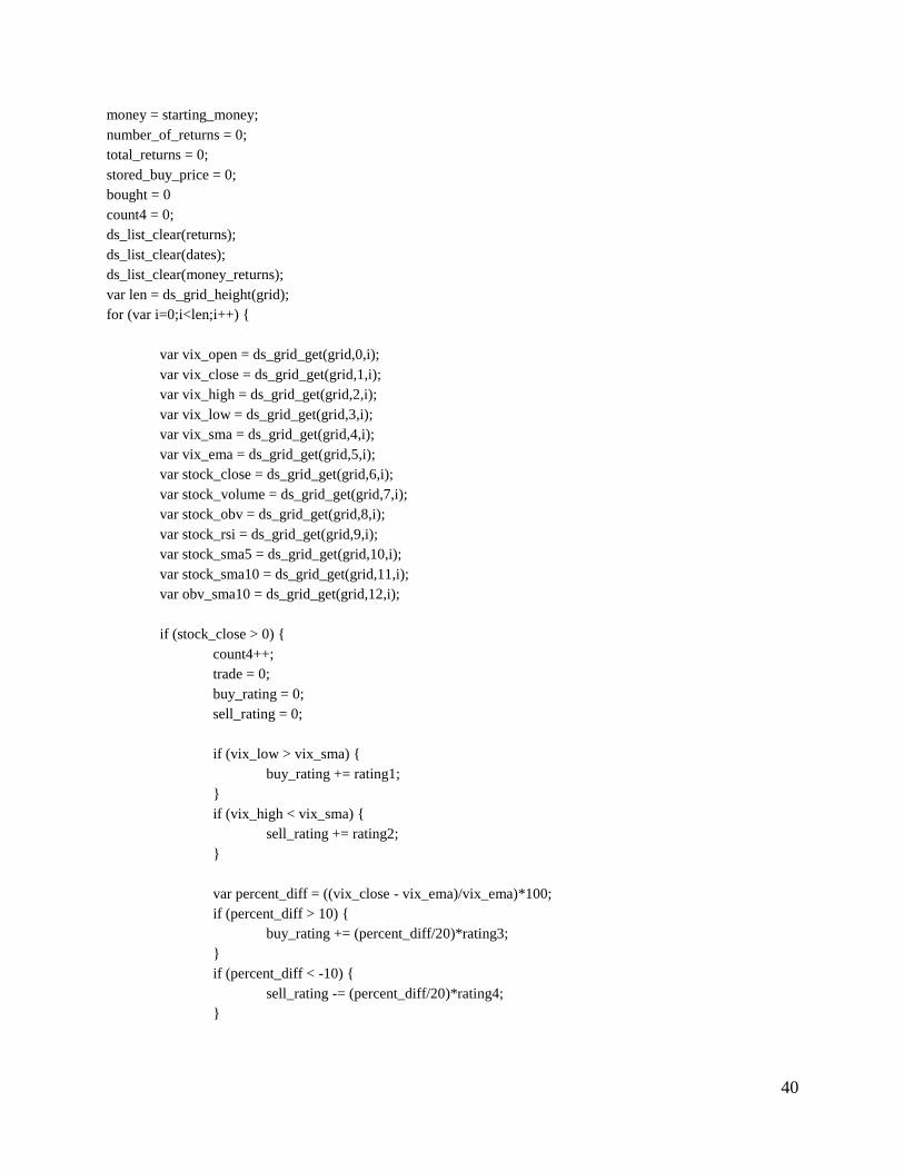
40
money = starting_money;
number_of_returns = 0;
total_returns = 0;
stored_buy_price = 0;
bought = 0
count4 = 0;
ds_list_clear(returns);
ds_list_clear(dates);
ds_list_clear(money_returns);
var len = ds_grid_height(grid);
for (var i=0;i<len;i++) {
var vix_open = ds_grid_get(grid,0,i);
var vix_close = ds_grid_get(grid,1,i);
var vix_high = ds_grid_get(grid,2,i);
var vix_low = ds_grid_get(grid,3,i);
var vix_sma = ds_grid_get(grid,4,i);
var vix_ema = ds_grid_get(grid,5,i);
var stock_close = ds_grid_get(grid,6,i);
var stock_volume = ds_grid_get(grid,7,i);
var stock_obv = ds_grid_get(grid,8,i);
var stock_rsi = ds_grid_get(grid,9,i);
var stock_sma5 = ds_grid_get(grid,10,i);
var stock_sma10 = ds_grid_get(grid,11,i);
var obv_sma10 = ds_grid_get(grid,12,i);
if (stock_close > 0) {
count4++;
trade = 0;
buy_rating = 0;
sell_rating = 0;
if (vix_low > vix_sma) {
buy_rating += rating1;
}
if (vix_high < vix_sma) {
sell_rating += rating2;
}
var percent_diff = ((vix_close - vix_ema)/vix_ema)*100;
if (percent_diff > 10) {
buy_rating += (percent_diff/20)*rating3;
}
if (percent_diff < -10) {
sell_rating -= (percent_diff/20)*rating4;
}
41
if (vix_close < 13) {
buy_rating += 0.5*(13-vix_close)*rating5;
}
if (vix_close > 25) {
sell_rating += 0.5*(vix_close-25)*rating6;
}
if (extra_indicators) {
if (stock_rsi > 65) {
sell_rating += (0.2*(stock_rsi-65)*rating9);
}
if (stock_rsi < 35) {
buy_rating += (0.2*(35-stock_rsi)*rating10);
}
}
if (i > 0) {
var vix_close_prev = ds_grid_get(grid,1,i-1);
var vix_change = ((vix_close - vix_close_prev)/vix_close_prev)*100;
if (vix_change > 9) {
buy_rating += 0.2*(vix_change-9)*rating7;
}
if (vix_change < -9) {
sell_rating -= 0.2*(vix_change+9)*rating8;
}
if (extra_indicators) {
var stock_sma5_prev = ds_grid_get(grid,10,i-1);
var stock_sma10_prev = ds_grid_get(grid,11,i-1);
if (stock_sma5 > stock_sma10 && stock_sma5_prev < stock_sma10_prev) {
buy_rating += rating11;
} else if (stock_sma5 < stock_sma10 && stock_sma5_prev > stock_sma10_prev) {
sell_rating += rating12;
}
}
}
if (extra_indicators) {
if (i > 9) {
var slopea1 = stock_sma10;
var slopea2 = ds_grid_get(grid,11,i-10);
var slopeb1 = obv_sma10;
var slopeb2 = ds_grid_get(grid,12,i-10);
var stock_slope = ((slopea1-slopea2)/slopea2)*100;
var obv_slope = ((slopeb1-slopeb2)/slopeb2)*100;
42
var slope = 7;
var diff = 5;
if (stock_slope > slope) {
if (abs(stock_slope - obv_slope) < diff) {
buy_rating += 3;
} else if (obv_slope < stock_slope) {
sell_rating += 3;
}
} else if (stock_slope < -slope) {
if (abs(stock_slope - obv_slope) < diff) {
sell_rating += 3;
} else if (obv_slope > stock_slope) {
buy_rating += 3;
}
} else {
if (abs(stock_slope - obv_slope) < diff) {
} else if (obv_slope > stock_slope) {
buy_rating += 3;
} else if (obv_slope < stock_slope) {
sell_rating += 3;
}
}
}
}
if (i==0 && bought == 0) {
stored_buy_price = stock_close;
bought = 1;
money -= 7;
} else if (((i >= 113) || (sell_rating > rating14)) && bought == 1) {
bought = 0;
percent_return = ((stock_close-stored_buy_price)/stored_buy_price)*100;
ds_list_add(returns,percent_return);
ds_list_add(dates,i);
money += (percent_return/100)*money;
ds_list_add(money_returns,money);
money -= 7;
}
}
}
for (var i=0;i<ds_list_size(returns);i++) {
number_of_returns++;
var ret = ds_list_find_value(returns,i);
43
total_returns += ret;
}
mean_returns = total_returns/number_of_returns;
}
delay++;
if (simulate) {
delay = 0;
count = 0;
simulate = 0;
update = 1;
var r1 = rating1;
var r2 = rating2;
var r3 = rating3;
var r4 = rating4;
var r5 = rating5;
var r6 = rating6;
var r7 = rating7;
var r8 = rating8;
var r9 = rating9;
var r10 = rating10;
var r11 = rating11;
var r12 = rating12;
var r13 = rating13;
var r14 = rating14;
range1 = -15;
range2 = 20;
switch (state) {
case 14:
range1 = 5;
range2 = 30;
break;
case 15:
range1 = 5;
range2 = 30;
break;
}
for (var i=range1;i<range2;i+=(range2-range1)/accuracy) {
switch (state) {
case 2:
r1 = i;
44
break;
case 3:
r2 = i;
break;
case 4:
r3 = i;
break;
case 5:
r4 = i;
break;
case 6:
r5 = i;
break;
case 7:
r6 = i;
break;
case 8:
r7 = i;
break;
case 9:
r8 = i;
break;
case 10:
r9 = i;
break;
case 11:
r10 = i;
break;
case 12:
r11 = i;
break;
case 13:
r12 = i;
break;
case 14:
r13 = i;
break;
case 15:
r14 = i;
break;
}
money = starting_money;
number_of_returns = 0;
total_returns = 0;
stored_buy_price = 0;
bought = 0
ds_list_clear(returns);

45
ds_list_clear(dates);
ds_list_clear(money_returns);
var len = ds_grid_height(grid);
for (var j=0;j<len;j++) {
var vix_open = ds_grid_get(grid,0,j);
var vix_close = ds_grid_get(grid,1,j);
var vix_high = ds_grid_get(grid,2,j);
var vix_low = ds_grid_get(grid,3,j);
var vix_sma = ds_grid_get(grid,4,j);
var vix_ema = ds_grid_get(grid,5,j);
var stock_close = ds_grid_get(grid,6,j);
var stock_volume = ds_grid_get(grid,7,j);
var stock_obv = ds_grid_get(grid,8,j);
var stock_rsi = ds_grid_get(grid,9,j);
var stock_sma5 = ds_grid_get(grid,10,j);
var stock_sma10 = ds_grid_get(grid,11,j);
var obv_sma10 = ds_grid_get(grid,12,j);
if (stock_close > 0) {
trade = 0;
buy_rating = 0;
sell_rating = 0;
if (vix_low > vix_sma) {
buy_rating += r1;
}
if (vix_high < vix_sma) {
sell_rating += r2;
}
var percent_diff = ((vix_close - vix_ema)/vix_ema)*100;
if (percent_diff > 10) {
buy_rating += (percent_diff/20)*r3;
}
if (percent_diff < -10) {
sell_rating -= (percent_diff/20)*r4;
}
if (vix_close < 13) {
buy_rating += 0.5*(13-vix_close)*r5;
}
if (vix_close > 25) {
sell_rating += 0.5*(vix_close-25)*r6;
}
if (extra_indicators) {
if (stock_rsi > 65) {
46
sell_rating += (0.2*(stock_rsi-65)*r9);
}
if (stock_rsi < 35) {
buy_rating += (0.2*(35-stock_rsi)*r10);
}
}
if (j > 0) {
var vix_close_prev = ds_grid_get(grid,1,j-1);
var vix_change = ((vix_close - vix_close_prev)/vix_close_prev)*100;
if (vix_change > 9) {
buy_rating += 0.2*(vix_change-9)*r7;
}
if (vix_change < -9) {
sell_rating -= 0.2*(vix_change+9)*r8;
}
if (extra_indicators) {
var stock_sma5_prev = ds_grid_get(grid,10,j-1);
var stock_sma10_prev = ds_grid_get(grid,11,j-1);
if (stock_sma5 > stock_sma10 && stock_sma5_prev < stock_sma10_prev) {
buy_rating += r11;
} else if (stock_sma5 < stock_sma10 && stock_sma5_prev > stock_sma10_prev) {
sell_rating += r12;
}
}
}
if (extra_indicators) {
if (j > 9) {
var slopea1 = stock_sma10;
var slopea2 = ds_grid_get(grid,11,j-10);
var slopeb1 = obv_sma10;
var slopeb2 = ds_grid_get(grid,12,j-10);
var stock_slope = ((slopea1-slopea2)/slopea2)*100;
var obv_slope = ((slopeb1-slopeb2)/slopeb2)*100;
var slope = 7;
var diff = 5;
if (stock_slope > slope) {
if (abs(stock_slope - obv_slope) < diff) {
buy_rating += 3;
} else if (obv_slope < stock_slope) {
sell_rating += 3;
}
} else if (stock_slope < -slope) {
if (abs(stock_slope - obv_slope) < diff) {
sell_rating += 3;
47
} else if (obv_slope > stock_slope) {
buy_rating += 3;
}
} else {
if (abs(stock_slope - obv_slope) < diff) {
} else if (obv_slope > stock_slope) {
buy_rating += 3;
} else if (obv_slope < stock_slope) {
sell_rating += 3;
}
}
}
}
if (buy_rating > r13 && bought == 0) {
stored_buy_price = stock_close;
bought = 1;
money -= 7;
} else if (((i == len) || (sell_rating > r14)) && bought == 1) {
bought = 0;
percent_return = ((stock_close-stored_buy_price)/stored_buy_price)*100;
ds_list_add(returns,percent_return);
ds_list_add(dates,i);
money += (percent_return/100)*money;
ds_list_add(money_returns,money);
money -= 7;
}
}
}
for (var w=0;w<ds_list_size(returns);w++) {
number_of_returns++;
var ret = ds_list_find_value(returns,w);
total_returns += ret;
}
mean_returns = total_returns/number_of_returns;
graph[count] = money/600;
count++;
if (money > highest_returns) {
highest_returns = money;
rating1 = r1;
rating2 = r2;
rating3 = r3;
48
rating4 = r4;
rating5 = r5;
rating6 = r6;
rating7 = r7;
rating8 = r8;
rating9 = r9;
rating10 = r10;
rating11 = r11;
rating12 = r12;
rating13 = r13;
rating14 = r14;
}
}
}