UNIVERSITY OF CALIFORNIA

Santa Barbara

Exploring Transition Trajectory from Quadrupedal Stance Using ZMP Based Bang-

Bang Control and Quadratic Programming

A Thesis submitted in partial satisfaction of the

requirements for the degree Master of Science

in Electrical and Computer Engineering

by

Howard Yu-Hao Hu

Committee in charge:

Professor Katie Byl, Chair

Professor Francesco Bullo

Professor Joao Hespanha

March 2014

The thesis of Howard Yu-Hao Hu is approved.

____________________________________________

Francesco Bullo

____________________________________________

Joao Hespanha

____________________________________________

Katie Byl, Committee Chair

Dec 2013

iii

Exploring Transition Trajectory from Quadrupedal Stance Using ZMP Based Bang-

Bang Control and Quadratic Programming

Copyright © 2014

by

Howard Yu-Hao Hu

iv

ACKNOWLEDGEMENTS

First, I would like to thank my thesis advisor, Katie Byl. During the past year

working at the UCSB Robotics Lab, Katie has provided me with tremendous

guidance and mentorship. From knowing little about legged robots to finishing this

thesis, I had her by my side answering and discussing the retails of the research. I

would also like to thank my committee members, Joao Hespanha and Francesco

Bullo, for the knowledge they passed on through their courses in Control and

Robotics at UCSB.

The inputs from many of my colleagues have helped me through each step of my

research and life as a master student. In particular, Peter Ha with his inspiration has

led me to concentrate on the work whenever I have doubts. Also, thanks to all the

friends at UCSB who have made my life away from my hometown fun and

memorable.

Finally, thanks to my parents, sister and Nicole Chen who have supported me in

every possible way throughout the Master’s program and especially when I was in

stress trying to finish the thesis.

v

ABSTRACT

Exploring Transition Trajectory from Quadrupedal Stance Using ZMP Based Bang-

Bang Control and Quadratic Programming

by

Howard Yu-Hao Hu

Both quadrupedal and bipedal robots have their own advantages. In order for

some quadrupedal robots, such as Jet Propulsion Laboratory’s RoboSimian, to act as

bipedal robots, a transition motion is often needed. In this thesis, we present a ZMP

based bang-bang control method to solve for a minimum time transition trajectory

for a simplified dynamic model. Also, we explore two different quadratic

programming problem formulations to plan for a fast pitching up robot trajectory

from being horizontal in hope that the robot can be balanced when it’s near an

upright position. We also investigate different ways to improve the speed a body

trajectory given a limited physical capability of a robot.

vi

TABLE OF CONTENTS

I. Introduction ................................................................................................. 1

II. Background ................................................................................................. 4

A. Stability ............................................................................................. 4

i. Statically Stable ............................................................................. 4

ii. Dynamically Stable ....................................................................... 5

B. Ground Reaction Forces .................................................................... 8

III. ZMP Based Bang-Bang Control Planning ................................................ 12

IV. Quadrupedal Robot Transitioning ............................................................. 15

A. Framework 1: Quadratic Programming .......................................... 16

i. Optimization ................................................................................ 16

ii. Cost Functions ............................................................................. 17

iii. Approach ..................................................................................... 18

B. Framework 2: Two-Pass Quadratic Programming .......................... 22

i. Approach ..................................................................................... 22

V. Experiment ................................................................................................ 23

A. RoboSimian ..................................................................................... 23

B. Test Setup ........................................................................................ 24

C. COM Estimation Models for ZMP ................................................. 25

VI. Results ....................................................................................................... 27

A. Compare QP and 2-Pass QP ............................................................ 27

B. In the case where we allow Z height to change............................... 33

vii

C. Limited Capability (speed and velocity cap) .................................. 35

VII. Conclusion ................................................................................................. 37

VIII. Future Work .............................................................................................. 39

References ................................................................................................................... 40

viii

LIST OF FIGURES

Figure 1 Support Polygon ............................................................................................. 5

Figure 2 Cart-Table Model ............................................................................................ 7

Figure 3 Ground Reaction Force Distribution ............................................................ 10

Figure 4 Factors for Slippage with = 0.3 ........................................................... 11

Figure 5 Phase Plot for a Bang-Bang Control in ZMP ............................................... 14

Figure 6 Flowchart for QP approach for Pose Transitioning ...................................... 21

Figure 7 RoboSimian Conceptual Art ......................................................................... 23

Figure 8 COB Trajectory using QP Approach ............................................................ 27

Figure 9 Resultant COM and ZMP Trajectory using QP Approach ........................... 28

Figure 10 Minimum ................................................................................................. 28

Figure 11 Resultant COM and ZMP Trajectory using 2-Pass QP Approach ............. 31

Figure 12 MATLAB Simulation from QP Results ..................................................... 32

Figure 13 ZMP Trajectory with Bounding ZMP approach. ........................................ 33

Figure 14 ZMP Trajectory With Varying Z Height .................................................... 34

Figure 15 Different Joint Velocities ............................................................................ 36

1

I. Introduction

Different locomotion mechanisms are designed for a robot to traverse effectively

through different categories of environments. While wheeled robots can be quite

efficient and agile in moving around a wide variety of relatively smooth and level

surfaces, legged robots tend to be more suitable for rougher terrains, particularly

where terrain has discontinuities such as gaps or stair-like features. Legged robots

often attempted to imitate biological systems, and they can be categorized by the

number of legs they possess. Out of all the different legged robots, studying of

human-like bipedal walking robots and dog-like quadrupedal robots are the two main

research areas [14]. Asimo and Nao are a few commonly known examples of robots

that are inspired by humans. Humanoid robots are more socially acceptable due to

their appearances, and some, such as powered exoskeleton, can even provide

assistance in human strength and endurance [12] or gait rehabilitation [15]. One of

the benefits for robots to take on a humanoid form is to be able to operate in the

same spaces and using the same tools designed by and for humans. For example, a

robot that stands on two feet occupies only a small footprint on the ground and can

move about while its hands are used for different manipulation tasks. On the other

hand, a robot that walks on all the limbs can maneuver in a more stable gait.

In order to take advantage of both sides, transitioning between two modes of

locomotion can be useful and this behavior is commonly observed in nature when

animals are trying to overcome and adapt to different environments. For example,

2

children who have just learned to walk often switch back to crawling when they are

climbing stairs or weaving through rough terrains. On the other hand, grizzly bears

normally walk on all four limbs, yet they stand on their hind legs when they start to

climb trees.

Most quadrupedal robots without either large feet for support or hands to grasp to

environment, such as LittleDog [5], rarely stand to free up the front appendages

because a stable pose usually requires for at least three feet are used to form a

support polygon on the ground. Hence, transitioning from crawling to standing is

typically performed by humanoid robots because they are more capable of

performing various manipulation tasks [8][9][10].

Inspired by both the four-legged and two-legged robots and the advantage of

each, we want to look into a fast transition motion from a quadrupedal stance to a

pitched up bipedal pose with the help of hands pushing against a wall. In this thesis,

different methods to plan for a fast trajectory using quadratic programming are

exploited. Similar methods have been used in the field to plan for a walking gait [5]

or a robot balancing [11]. First, Section II introduces background information on

several terminologies and criteria for robot trajectory planning. Next, Section III

discusses a trajectory for transitioning using a modified bang-bang control method

that switches between two extreme ends of ZMP locations instead of the traditional

method of switching the magnitude of the acceleration. Two formulations and

implementations of quadratic programming problems for planning a transition

motion are presented in Section IV. Section V and VI talk about the simulation setup

3

for the problem and the results for the quadratic programming solver. Lastly, the

conclusion of the thesis is summarized in Section VII and possible future work is

discussed in Section VIII.

4

II. Background

A. Stability

In robot motion planning, stability is one of the most critical requirements.

Robots simply cannot operate properly if they fall or tip over while tracking

trajectories or performing certain actions. Needless to say, most robots capable of

complex manipulation tasks are expensive and fragile and can easily be damaged

through rough and unforeseen impacts. Hence, stability criteria are analyzed to

prevent such things from happening.

i. Statically Stable

Static stability requires a safety margin between a robot’s center of mass (COM)

projected onto a ground plane and a convex hull enclosed by points on the robot

contacting the ground. This region formed by the contacting points is called a

support polygon (SP), and it is used to determine both static and dynamic stability.

An illustration of SP can be found in Figure 1. For a robot at rest, if the projection of

the stationary COM is within the convex hull of the support polygon, the robot is

known as statically stable, meaning there are no tipping moments about any edge of

the support polygon and the robot will not fall. The static stability margin is also

frequently used for robots that move relatively slowly, because the COM will be

very close to the center of pressure (COP) of the robot if robot accelerations are

small enough. However, this criterion is not sufficient once the movement is faster

and the dynamic behavior becomes significant.

5

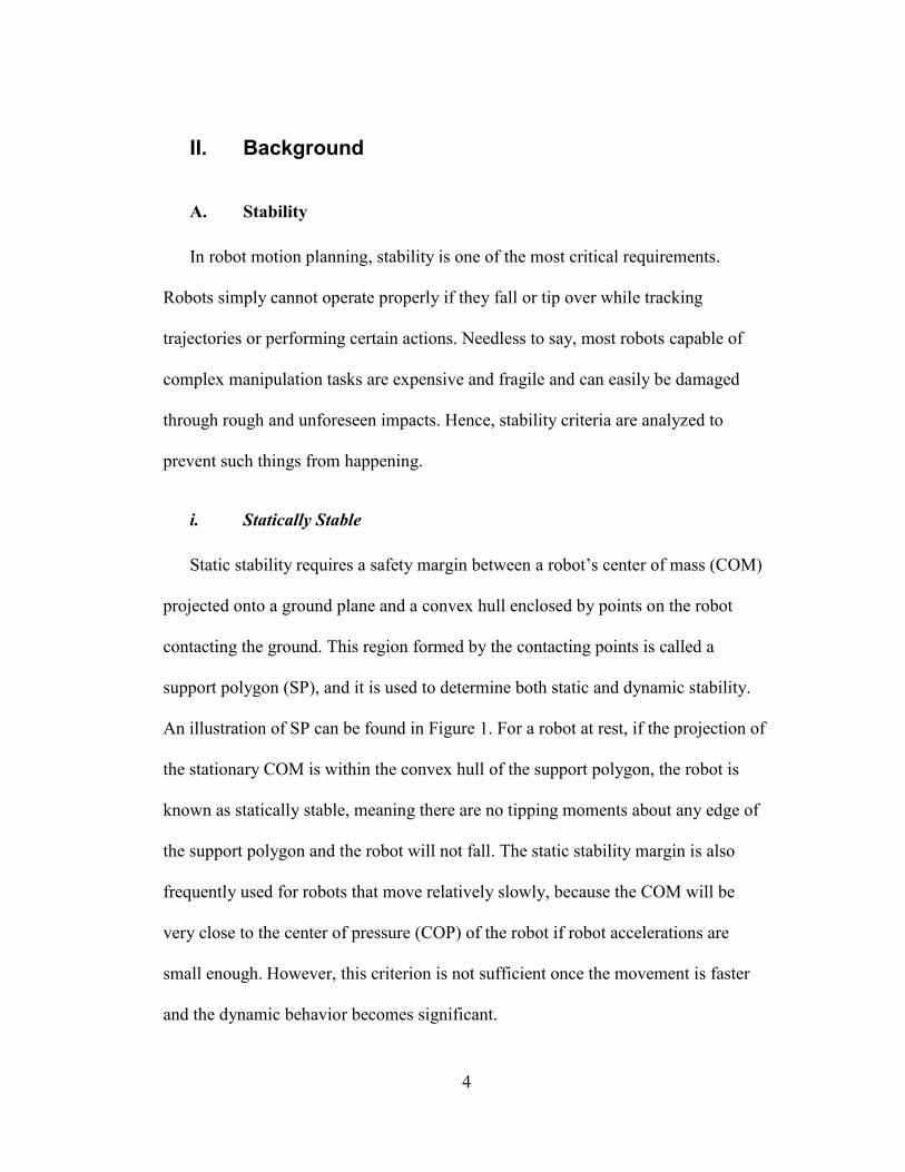
Figure 1 Support Polygon

A support polygon is shaded with black stripes and the foothold location is

colored in red. The left figure is in double support with both feet are on the

ground, and the right figure shows single support with one foot lifted off the

ground. If COG falls onto the shaded area in either case, a robot is in static

stable mode.

ii. Dynamically Stable

Zero Moment Point (ZMP) was introduced in late 1960’s by Miomir

Vulobratovic [1] as a measure for locomotion stability. As the name suggests, the

ZMP is a point where the total amount of torque produced by external forces on the

robot equals to zero. The ZMP is more commonly known as the center of pressure

(COP). In robotics, the term ZMP is often used when considering a particular set of

motions for a robot to determine dynamic feasibility given the planned contacts

between the robot and the external world. For a given, prescribed set of desired

motions for a robot, one can calculate the location, direction and magnitude of the

net force vector provided by the external world simply using Newton’s second law.

The ZMP must lie somewhere along the line formed by this vector in space. Visually,

6

one can imagine all the planned internal motions of the robot can be achieved if the

external world pushes exactly along this line, e.g. with a long stick, perhaps also with

a twisting moment about the axis of the stick, but with no net moment about any

other axis. The point where this stick-axis intersects the ground is the required ZMP

location for the planned motions. If this point is inside the support polygon, then the

planned motions are dynamically feasible. If this point is outside of the support

polygon, the planned motions are not feasible, the actual COP (aka ZMP) will fall

exactly on the edge of the support polygon, and the robot will tip more than planned

about this SP edge. The use of the term "ZMP" instead of "COP" traditionally

indicates that motions are planned first, with the required ZMP calculated as a means

of verifying feasibility, while COP is usually used in the context of measurements of

force on the ground.

The criterion of ZMP analyzes dynamic effects of positions, accelerations, and

rotation during any movement. A fictitious ZMP is a planned point outside of the

support polygon which cannot exist as no ground reaction force can act at such a

point. However, a fictitious ZMP can be used for planning if one chooses to exploit

an underactuated, tipping motion in the robot [4].

7

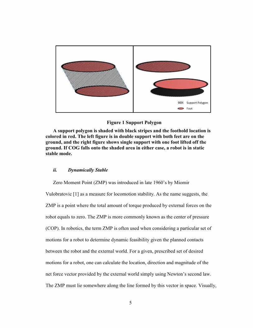
Figure 2 Cart-Table Model

For a planer model, ZMP with an effect of inertia [6] can be calculated as

∑ ( ( ) )

∑ ( )

(II.1)

where indicates each point on a robot, is the mass of each link on a robot, is

the inertial components, is angular acceleration. Kajita et al. has also provided a

simplified cart-table model [7] to compute ZMP that assumes the COM is always at

a constant Z height with only a single point mass and it is shown as,

(II.2)

where and is the location of center of mass, g is the gravitational

acceleration, and is the acceleration in X. This assumption of having a constant

8

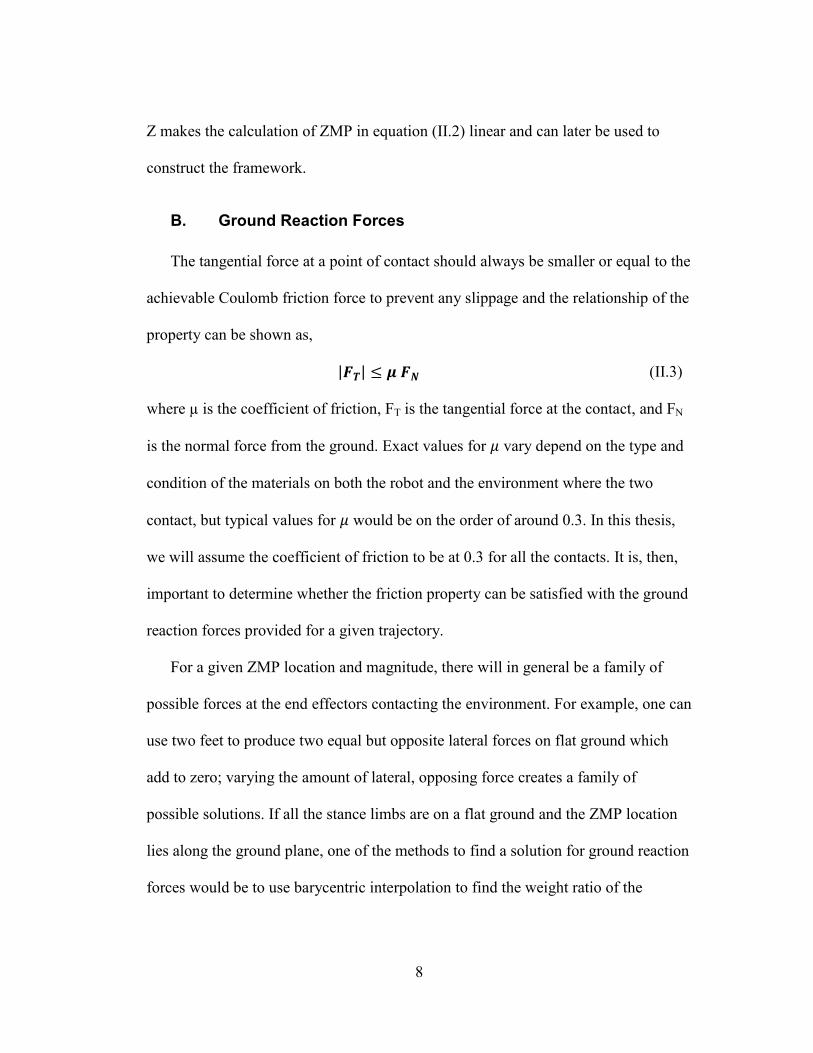
Z makes the calculation of ZMP in equation (II.2) linear and can later be used to

construct the framework.

B. Ground Reaction Forces

The tangential force at a point of contact should always be smaller or equal to the

achievable Coulomb friction force to prevent any slippage and the relationship of the

property can be shown as,

| | (II.3)

where µ is the coefficient of friction, FT is the tangential force at the contact, and FN

is the normal force from the ground. Exact values for vary depend on the type and

condition of the materials on both the robot and the environment where the two

contact, but typical values for would be on the order of around 0.3. In this thesis,

we will assume the coefficient of friction to be at 0.3 for all the contacts. It is, then,

important to determine whether the friction property can be satisfied with the ground

reaction forces provided for a given trajectory.

For a given ZMP location and magnitude, there will in general be a family of

possible forces at the end effectors contacting the environment. For example, one can

use two feet to produce two equal but opposite lateral forces on flat ground which

add to zero; varying the amount of lateral, opposing force creates a family of

possible solutions. If all the stance limbs are on a flat ground and the ZMP location

lies along the ground plane, one of the methods to find a solution for ground reaction

forces would be to use barycentric interpolation to find the weight ratio of the

9

resultant force on each of the limb in contact with the ground. Based on the weight

ratio, the contact forces along the axis of net force on the robot body can be

determined, and the lateral forces can be chosen to satisfy the minimum requirement

of the friction coefficient.

For a simplified planer model with the feet in contact with external objects

(either the ground or the walls), a distribution of ground reaction forces can be

determined through balancing forces and moments about the COP.

∑ (II.4)

∑ , i = 1, … N (II.5)

where is a vector from the location of COP location to each location of

ground reaction forces, are the ground reaction forces, is a resultant force of all

the ground reaction forces, and is the number of contact points.

However, having a set of three equations and four unknowns, as shown in Figure

3, there can be multiple solutions for the force distribution. The 4th

unknown can be

represented by a free variable via the method of Gaussian elimination. To search for

any solution that obeys the friction property, we can solve for a set of feasible

solutions for the 4th

unknown and determine the minimum µ required by utilizing the

friction equation (II.3) and coordinate transformation for different angles of contact.

Alternatively, this can be formulated as a linear optimization problem that finds a

solution with the minimum required coefficient of friction.

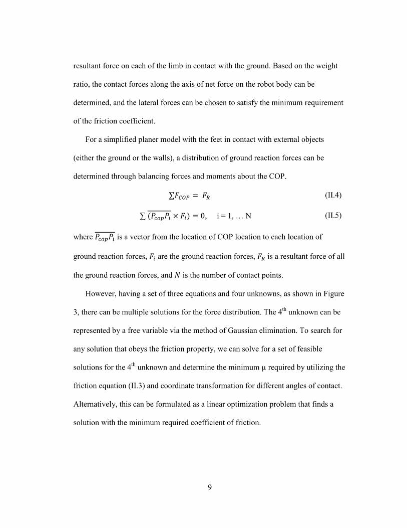
10

Figure 3 Ground Reaction Force Distribution

As shown in Figure 3, the front limb has a higher tendency to slip because

can often be very large in order to support robot’s weight while is related to

acceleration in X which is usually much less than gravitational acceleration. Given a

similar setup as shown in Figure 3, Figure 4 shows a few factors that can affect the

minimum coefficient of friction needed before encountering slippage. First, the

location of ZMP affects the distribution of the GRF; by putting more weight on the

back, it eases off the need to have larger . Similar to the ZMP location, the height

of the front limb forces to be large to balance the torque equation and hence it

requires a much smaller . Lastly, the larger the given the same the

smaller is needed.

11

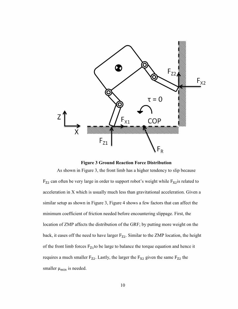
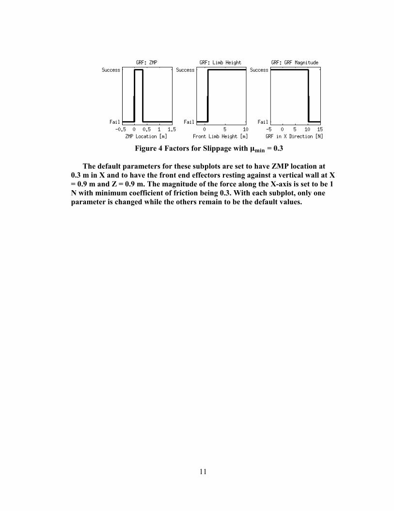
Figure 4 Factors for Slippage with = 0.3

The default parameters for these subplots are set to have ZMP location at

0.3 m in X and to have the front end effectors resting against a vertical wall at X

= 0.9 m and Z = 0.9 m. The magnitude of the force along the X-axis is set to be 1

N with minimum coefficient of friction being 0.3. With each subplot, only one

parameter is changed while the others remain to be the default values.

12

III. ZMP Based Bang-Bang Control Planning

Given a problem like moving a cart from point A to point B along the X-axis

with zero initial and final velocity and acceleration as quickly as possible can be

described as a minimum time problem where there exists one solution that minimizes

a cost function of time in the form of,

[ ] ∫

(III.1)

where is the initial condition, is the set of input to produce the shortest time

trajectory and T is the total time required. The solution of such problem can often be

generalized to a bang-bang control as the optimal solution. A bang-bang control, or

often called on and off control, is to toggle between a maximum and minimum input

to a system to reach the final. The minimum time input in this toy example is

to use full throttle to accelerate the cart towards point B and then to apply the

maximum deceleration to reach the goal point.

If now we decide to put the same cart on a table similar to the scenario in Figure

2, stability of the whole system then becomes an important consideration. We can

incorporate the concept of ZMP and still apply a similar bang-bang control to this

particular problem. In order to apply the maximum inputs to the cart tipping over the

table, we affix the location of ZMP to either side of the support polygon which

means that the force acting on the cart will not be at a constant value but become

dependent to the location of the cart.

13

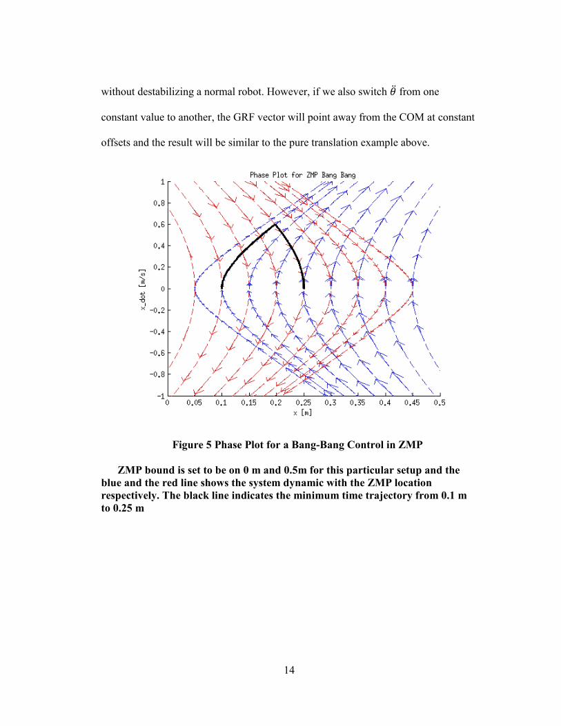
We simulated the system with one end of the ZMP at 0 m and the other end at

0.5 m with a mass of 100 kg. A ZMP solution is, however, independent of the mass

of the cart based on the equation (II.2). The phase plot of the system is shown in

Figure 5 where the blue lines indicate that the ZMP is located at the left most edge

and the red lines have the ZMP fixed to the right. We also simulate an example path

for a cart moving from 0.1 m to 0.25 using a minimum time switch policy and it can

be shown as a black line in the figure. Here we discard the area outside of the

allowable ZMP region as they will grow unbounded with initial velocity of zero.

From the phase plot, as the cart moves further away from the ZMP, the slope of the

figure becomes steeper and acceleration increases. This is because the ground

reaction force always points toward the center of mass in this system, since there are

no rotating inertias to support a net moment on the body, so the z component of force

always simply counteracts the acceleration of gravity, and the x component of force

on the body is therefore exactly proportional to the distance from the ZMP to the

COM in the x direction.

In addition, the solution will be very similar if we want to add in a change in

body pitch, , to the cart-table model to better demonstrate a robot transition motion.

Angular acceleration can be set arbitrarily large to allow for an arbitrarily large X

component to the GRF, because the GRF vector is no longer required to point at the

COM. Any net torque applied to the body simply balances with the instantaneous

angular acceleration of the body over time. This is not a practical solution in general

and would require a flywheel to help achieve the required angular accelerations

14

without destabilizing a normal robot. However, if we also switch from one

constant value to another, the GRF vector will point away from the COM at constant

offsets and the result will be similar to the pure translation example above.

Figure 5 Phase Plot for a Bang-Bang Control in ZMP

ZMP bound is set to be on 0 m and 0.5m for this particular setup and the

blue and the red line shows the system dynamic with the ZMP location

respectively. The black line indicates the minimum time trajectory from 0.1 m

to 0.25 m

15

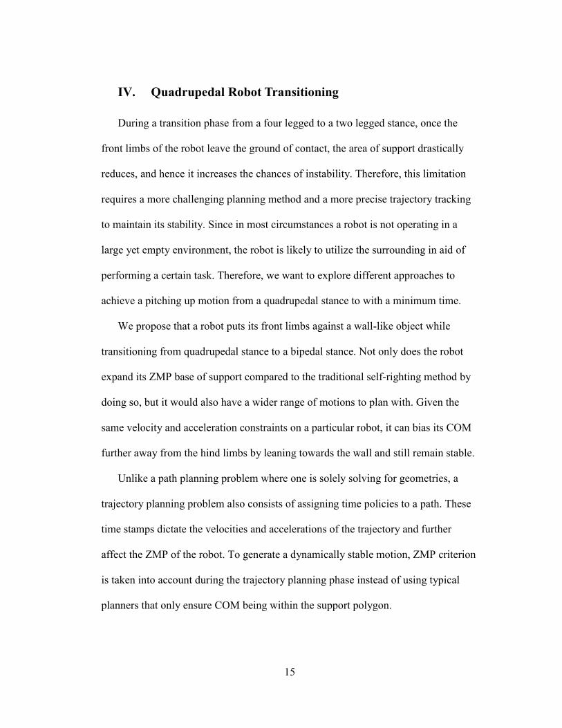
IV. Quadrupedal Robot Transitioning

During a transition phase from a four legged to a two legged stance, once the

front limbs of the robot leave the ground of contact, the area of support drastically

reduces, and hence it increases the chances of instability. Therefore, this limitation

requires a more challenging planning method and a more precise trajectory tracking

to maintain its stability. Since in most circumstances a robot is not operating in a

large yet empty environment, the robot is likely to utilize the surrounding in aid of

performing a certain task. Therefore, we want to explore different approaches to

achieve a pitching up motion from a quadrupedal stance to with a minimum time.

We propose that a robot puts its front limbs against a wall-like object while

transitioning from quadrupedal stance to a bipedal stance. Not only does the robot

expand its ZMP base of support compared to the traditional self-righting method by

doing so, but it would also have a wider range of motions to plan with. Given the

same velocity and acceleration constraints on a particular robot, it can bias its COM

further away from the hind limbs by leaning towards the wall and still remain stable.

Unlike a path planning problem where one is solely solving for geometries, a

trajectory planning problem also consists of assigning time policies to a path. These

time stamps dictate the velocities and accelerations of the trajectory and further

affect the ZMP of the robot. To generate a dynamically stable motion, ZMP criterion

is taken into account during the trajectory planning phase instead of using typical

planners that only ensure COM being within the support polygon.

16

Traditionally, the approach to plan a body motion is to slowly move the robot’s

COM on top of the support polygon and then extend and pitch the body upward. This

generates a desired COM trajectory to achieve an approximately upright pose while

remaining statically stable. This is similar to a traditional self-righting method of a

humanoid robot that carefully plans for center of mass locations [14]. However, this

motion is inherently slow and unstable due to a small support polygon [13].

Therefore, after solving for an inverse kinematic solution to obtain joint trajectories

of the robot, a speed knob can be adjusted on how fast the robot can play back the

desire trajectories and still maintain dynamic stablility.

In this section we will look at two methods to plan for faster body motions to

achieve a default standing pose from a quadrupedal stance. The first approach

formulates a ZMP constrained trajectory planner into a quadratic programming

problem based on a model of a floating box as a representation of a robot while the

second approach aims to improve a robot representation by formulating two

quadratic programming problems.

A. Framework 1: Quadratic Programming

i. Optimization

An optimization problem generally consists of the form

(IV.1)

17

where x is denoted as an n-dimensional column vector of variables that is being

optimized, is an objective function that is being minimized, is an m-dimensional

vector of functions for the constraints, and b is also an m-dimensional vector of

limits and bounds of the constraints. In particular, an optimization problem with

linear constraints and a quadratic objective function is called a quadratic

programming (QP). It obtains the general form (IV.1) with a quadratic convex

objective function as

where is an n-dimensional row vector for the linear term and is an n-by-n

positive semi-definite matrix for the quadratic term of the objective function.

ii. Cost Functions

An objective function quantifies a set of parameters into a single real number

which represents either a cost or a reward of an action. In the optimization problem

defined above, an objective function is being minimized and hence it is also called a

cost function. The solution of an optimization greatly depends on which cost

function is used. In this thesis, the cost function we explored minimizes the margin

between the ZMP location and the rear edge of the support polygon. This particular

cost function biases the COM location towards the rear limbs and redistributes the

ground reaction forces to minimize the chances of slipping. While this might seem

counter-intuitive in the sense that instability can potentially be induced, it can be

avoided by imposing an additional safety margin for ZMP.

18

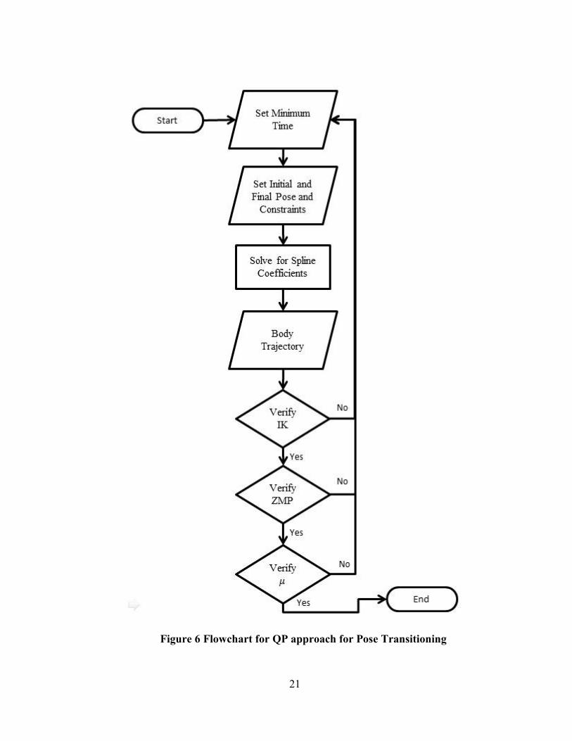
iii. Approach

The problem for transitioning from a quadrupedal pose to a bipedal pose can be

formulated as an optimization problem. A flowchart of the framework utilizing QP is

presented in Figure 6. Similar to generic motion planning, we first define initial and

final boundary conditions for the center of body (COB). In addition to that, the front

and the back end effector locations are heuristically chosen based on the free

configuration space of the body, free collision with the environment, and desired

ground reaction forces distribution.

Given the end conditions, we can use a QP solver to find a trajectory that

minimizes a designed objective function and complies with predefined ZMP

constraints. A sagittal plane approach is used in the problem, so the trajectory along

y-axis is assumed to be constant and we only have to consider a 2D model. Hence,

only x and z position and along with the pitch of center of body trajectory are then

formulated as a n-degree spline as

∑

(IV.1)

Where the term is the coefficient for spline and is the range variable of the

curve that usually goes from 0 to 1. term is used here instead of a time variable to

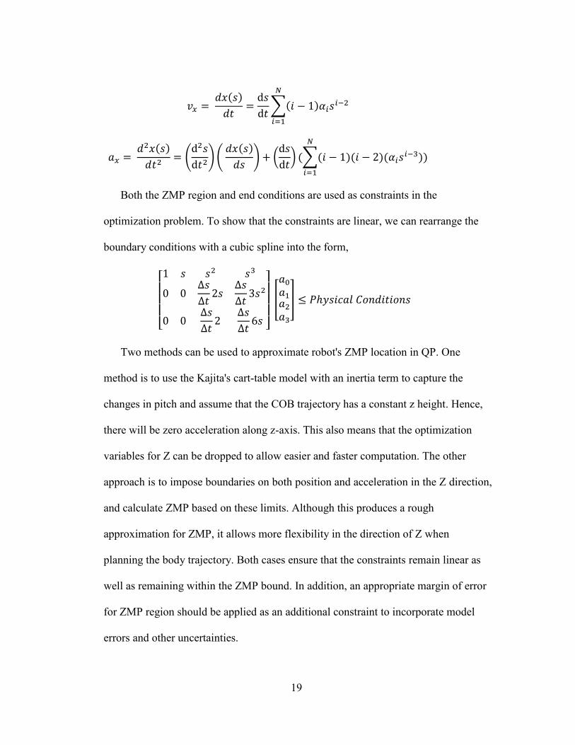
prevent computational error in higher dimensions. In addition, the velocity and

acceleration representations can be easily derived via calculus and product rule for

the ZMP calculation later.

19

∑

(

)(

) (

) ∑

Both the ZMP region and end conditions are used as constraints in the

optimization problem. To show that the constraints are linear, we can rearrange the

boundary conditions with a cubic spline into the form,

[

]

[

]

Two methods can be used to approximate robot's ZMP location in QP. One

method is to use the Kajita's cart-table model with an inertia term to capture the

changes in pitch and assume that the COB trajectory has a constant z height. Hence,

there will be zero acceleration along z-axis. This also means that the optimization

variables for Z can be dropped to allow easier and faster computation. The other

approach is to impose boundaries on both position and acceleration in the Z direction,

and calculate ZMP based on these limits. Although this produces a rough

approximation for ZMP, it allows more flexibility in the direction of Z when

planning the body trajectory. Both cases ensure that the constraints remain linear as

well as remaining within the ZMP bound. In addition, an appropriate margin of error

for ZMP region should be applied as an additional constraint to incorporate model

errors and other uncertainties.

20

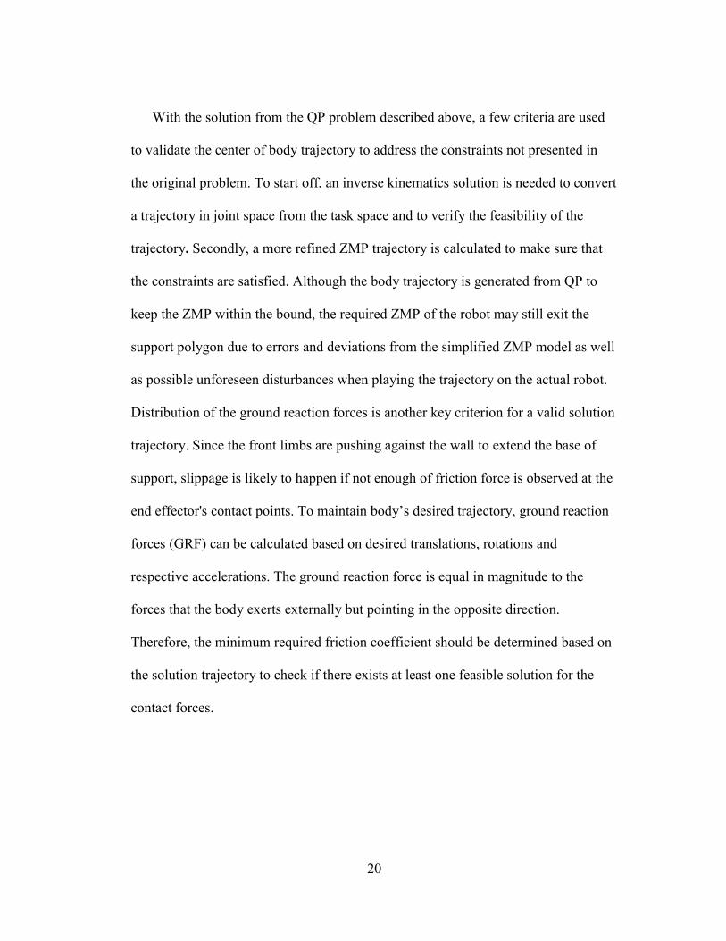
With the solution from the QP problem described above, a few criteria are used

to validate the center of body trajectory to address the constraints not presented in

the original problem. To start off, an inverse kinematics solution is needed to convert

a trajectory in joint space from the task space and to verify the feasibility of the

trajectory. Secondly, a more refined ZMP trajectory is calculated to make sure that

the constraints are satisfied. Although the body trajectory is generated from QP to

keep the ZMP within the bound, the required ZMP of the robot may still exit the

support polygon due to errors and deviations from the simplified ZMP model as well

as possible unforeseen disturbances when playing the trajectory on the actual robot.

Distribution of the ground reaction forces is another key criterion for a valid solution

trajectory. Since the front limbs are pushing against the wall to extend the base of

support, slippage is likely to happen if not enough of friction force is observed at the

end effector's contact points. To maintain body’s desired trajectory, ground reaction

forces (GRF) can be calculated based on desired translations, rotations and

respective accelerations. The ground reaction force is equal in magnitude to the

forces that the body exerts externally but pointing in the opposite direction.

Therefore, the minimum required friction coefficient should be determined based on

the solution trajectory to check if there exists at least one feasible solution for the

contact forces.

21

Figure 6 Flowchart for QP approach for Pose Transitioning

22

B. Framework 2: Two-Pass Quadratic Programming

The goal of this framework is to improve the ZMP model used in QP to account

for the difference between COB trajectory and COM trajectory, so that the resultant

ZMP trajectory can be closer to the desired one.

i. Approach

This approach is built on top of the concept in Section IV.A with one additional

quadratic programming problem in series. First we set up the same QP which outputs

a desired trajectory that satisfies the ZMP constraints calculated using the COB and

the body’s inertia. We then introduce a second pass QP that is almost identical to the

original one. From the solutions found in the first QP, we keep the Z and θ trajectory

the same as before and search through the trajectory only in X direction. This way,

we can re-calculate the ZMP location using an estimate of the COM with a 3-mass

model while the new the constraint statement remains linear. In Section V.C, we will

discuss more on the COM models.

23

V. Experiment

A. RoboSimian

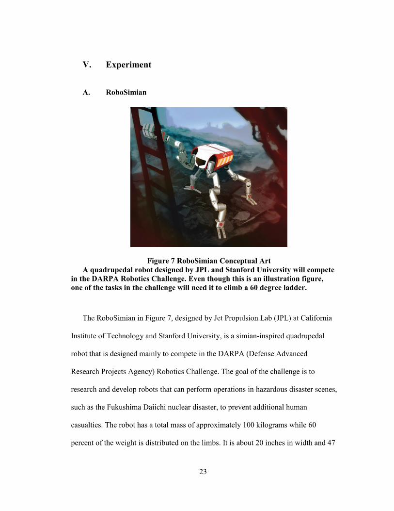
Figure 7 RoboSimian Conceptual Art

A quadrupedal robot designed by JPL and Stanford University will compete

in the DARPA Robotics Challenge. Even though this is an illustration figure,

one of the tasks in the challenge will need it to climb a 60 degree ladder.

The RoboSimian in Figure 7, designed by Jet Propulsion Lab (JPL) at California

Institute of Technology and Stanford University, is a simian-inspired quadrupedal

robot that is designed mainly to compete in the DARPA (Defense Advanced

Research Projects Agency) Robotics Challenge. The goal of the challenge is to

research and develop robots that can perform operations in hazardous disaster scenes,

such as the Fukushima Daiichi nuclear disaster, to prevent additional human

casualties. The robot has a total mass of approximately 100 kilograms while 60

percent of the weight is distributed on the limbs. It is about 20 inches in width and 47

24

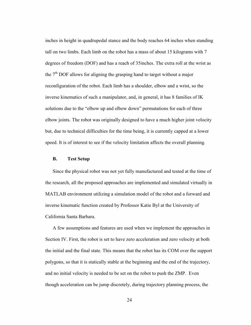
inches in height in quadrupedal stance and the body reaches 64 inches when standing

tall on two limbs. Each limb on the robot has a mass of about 15 kilograms with 7

degrees of freedom (DOF) and has a reach of 35inches. The extra roll at the wrist as

the 7th

DOF allows for aligning the grasping hand to target without a major

reconfiguration of the robot. Each limb has a shoulder, elbow and a wrist, so the

inverse kinematics of such a manipulator, and, in general, it has 8 families of IK

solutions due to the “elbow up and elbow down” permutations for each of three

elbow joints. The robot was originally designed to have a much higher joint velocity

but, due to technical difficulties for the time being, it is currently capped at a lower

speed. It is of interest to see if the velocity limitation affects the overall planning.

B. Test Setup

Since the physical robot was not yet fully manufactured and tested at the time of

the research, all the proposed approaches are implemented and simulated virtually in

MATLAB environment utilizing a simulation model of the robot and a forward and

inverse kinematic function created by Professor Katie Byl at the University of

California Santa Barbara.

A few assumptions and features are used when we implement the approaches in

Section IV. First, the robot is set to have zero acceleration and zero velocity at both

the initial and the final state. This means that the robot has its COM over the support

polygons, so that it is statically stable at the beginning and the end of the trajectory,

and no initial velocity is needed to be set on the robot to push the ZMP. Even

though acceleration can be jump discretely, during trajectory planning process, the

25

robot has a continuous acceleration as shown from equation (IV.1) for easier

computation and smaller jerk on the robot. As a result, we can see a relatively

smooth and continuous ZMP trajectory. As mentioned before, the robot is analyzed

in the sagittal plane and we assume that there is a decoupled relationship of ZMP

between the X and Y direction.

C. COM Estimation Models for ZMP

An estimate of the location of COM affects the accuracy of ZMP calculation, so

in this section we will look into three different methods with each having a different

complexity. The most primitive one is to assume that the robot carries all its weight

at the body location with a shape of a box for inertia and neglect the effects of all

other limbs. Despite the potential inaccuracy, this approach is commonly seen in

research such as for LittleDog due to its simplicities. The second method is to

approximate using 3-masses where the limb is assumed to also have a rectangular

shape that starts at the shoulder of the body to the end effector location. Comparing

to the first method, this allows us to account for the limbs’ dynamic when estimating

for the ZMP location since the limbs can often carry a large portion of the overall

weight. The last method, and also the most computationally heavy one, is to account

for all 15 links on the planer robot model where 1 is at the body and the rest are at

the front and rear limbs. A point mass is assumed to be at the center of each link and

it is decomposed into four points along the two principle rotational axes to account

for inertia. Although this ends up calculating for 60 masses, we will still refer it as a

15 masses approach for an indication of how many links are used. Throughout the

26

experiment, we compare the first two methods to the 15 masses as it is the best

representative of the true COM location.

27

VI. Results

A. Compare QP and 2-Pass QP

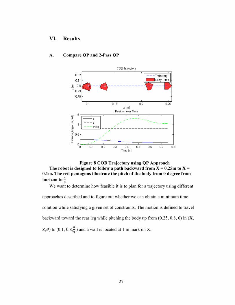
Figure 8 COB Trajectory using QP Approach

The robot is designed to follow a path backward from X = 0.25m to X =

0.1m. The red pentagons illustrate the pitch of the body from 0 degree from

horizon to

We want to determine how feasible it is to plan for a trajectory using different

approaches described and to figure out whether we can obtain a minimum time

solution while satisfying a given set of constraints. The motion is defined to travel

backward toward the rear leg while pitching the body up from (0.25, 0.8, 0) in (X,

Z, ) to (0.1, 0.8,

) and a wall is located at 1 m mark on X.

28

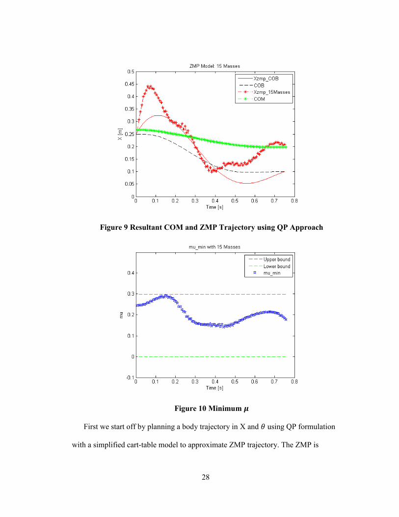
Figure 9 Resultant COM and ZMP Trajectory using QP Approach

Figure 10 Minimum

First we start off by planning a body trajectory in X and using QP formulation

with a simplified cart-table model to approximate ZMP trajectory. The ZMP is

29

calculated using only the COB dynamics during the planning process because COM

calculation requires using trigonometry on the optimization variables for and the

operation will not result in linear constraints. ZMP region is defined to be within a

support polygon from 0.05 m to 0.45m in X direction which has a 0.05 m of safety

margin on either edge. CVX program [2][3], a disciplined convex programming

solver in MATLAB, is then used to solve for the approach in Section IV.A. The cost

used in the section is to minimize the ZMP region to the rear limbs while finding the

minimum time to achieve so. Given the resultant COB trajectory shown in Figure 8,

Figure 9 shows the approximated ZMP and COM trajectory using the trajectories

from all 15 masses (14 masses for the 2 limbs and 1 mass for the body). Figure 10

shows the minimum time-varying magnitude of required to sustain the given ZMP

trajectory using the method described in Section B. A series of animation snapshots

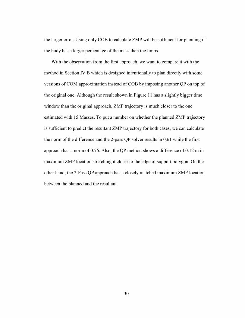
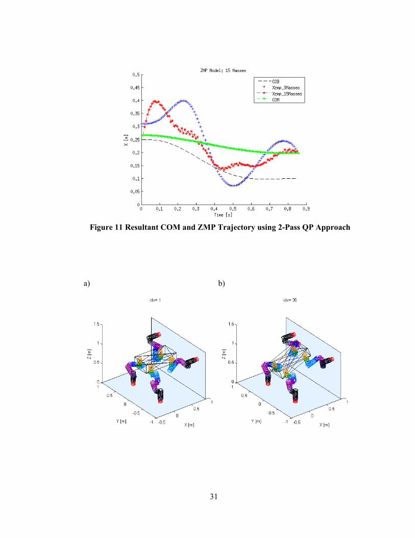
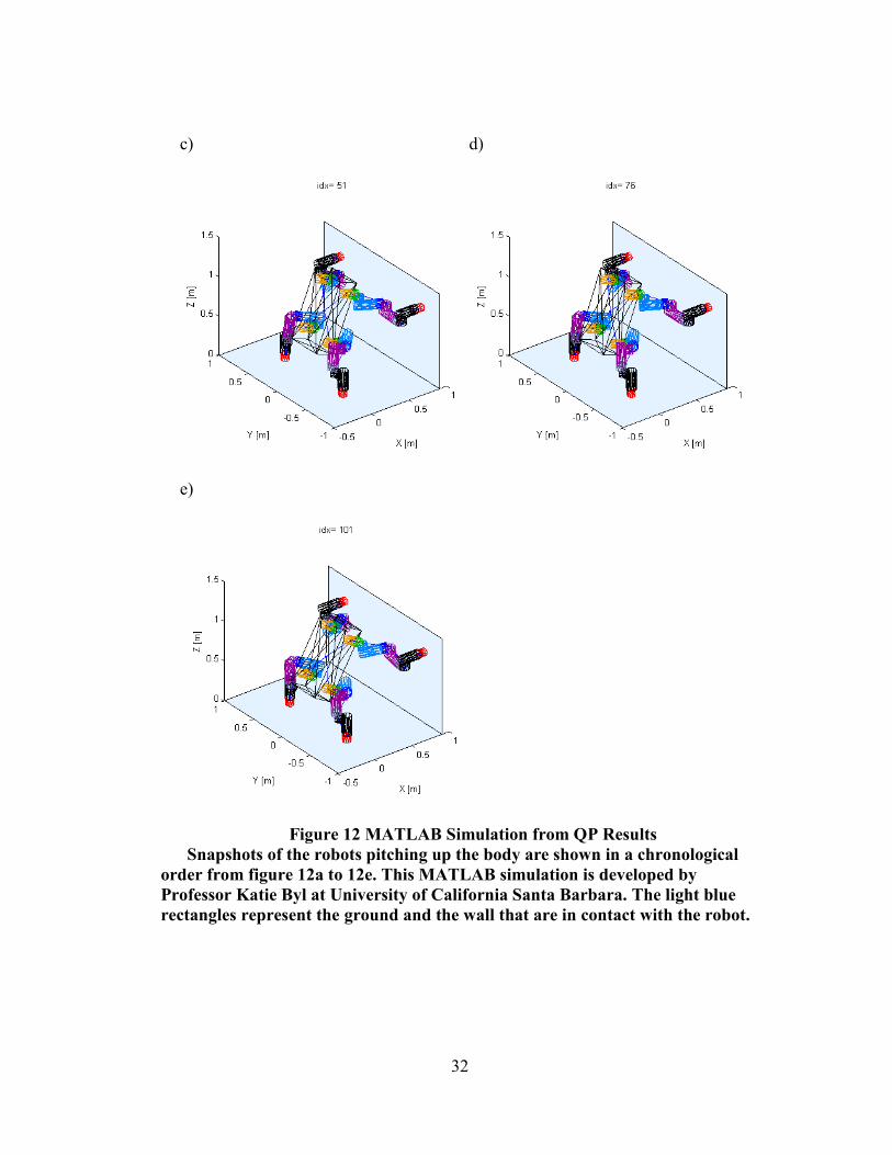
for the motion is presented in Figure 12. Without any physical limits on joint

velocity and joint acceleration, RoboSimian is capable of achieving the prescribed

path in 0.8 seconds while remaining stable. Even though this approach with the

particular setup can play back the motion within a short time window, it can be seen

that the deviation between COB and COM path is quite significant.

There is a bias of COM toward the front because the front limb has a significant

amount of mass and it acts like a hanging dead weight pushing the COM forward.

The difference grows larger as the pitch of the body becomes greater which results in

a more asymmetric geometry of the robot. In addition, both moving towards the rear

limb and reducing the body weight distribution along the X direction contribute to

30

the larger error. Using only COB to calculate ZMP will be sufficient for planning if

the body has a larger percentage of the mass then the limbs.

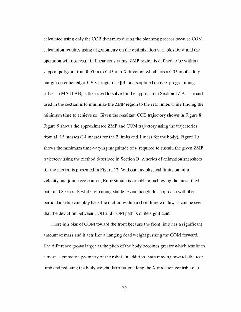
With the observation from the first approach, we want to compare it with the

method in Section IV.B which is designed intentionally to plan directly with some

versions of COM approximation instead of COB by imposing another QP on top of

the original one. Although the result shown in Figure 11 has a slightly bigger time

window than the original approach, ZMP trajectory is much closer to the one

estimated with 15 Masses. To put a number on whether the planned ZMP trajectory

is sufficient to predict the resultant ZMP trajectory for both cases, we can calculate

the norm of the difference and the 2-pass QP solver results in 0.61 while the first

approach has a norm of 0.76. Also, the QP method shows a difference of 0.12 m in

maximum ZMP location stretching it closer to the edge of support polygon. On the

other hand, the 2-Pass QP approach has a closely matched maximum ZMP location

between the planned and the resultant.

31

Figure 11 Resultant COM and ZMP Trajectory using 2-Pass QP Approach

a)

b)

32

c)

d)

e)

Figure 12 MATLAB Simulation from QP Results

Snapshots of the robots pitching up the body are shown in a chronological

order from figure 12a to 12e. This MATLAB simulation is developed by

Professor Katie Byl at University of California Santa Barbara. The light blue

rectangles represent the ground and the wall that are in contact with the robot.

33

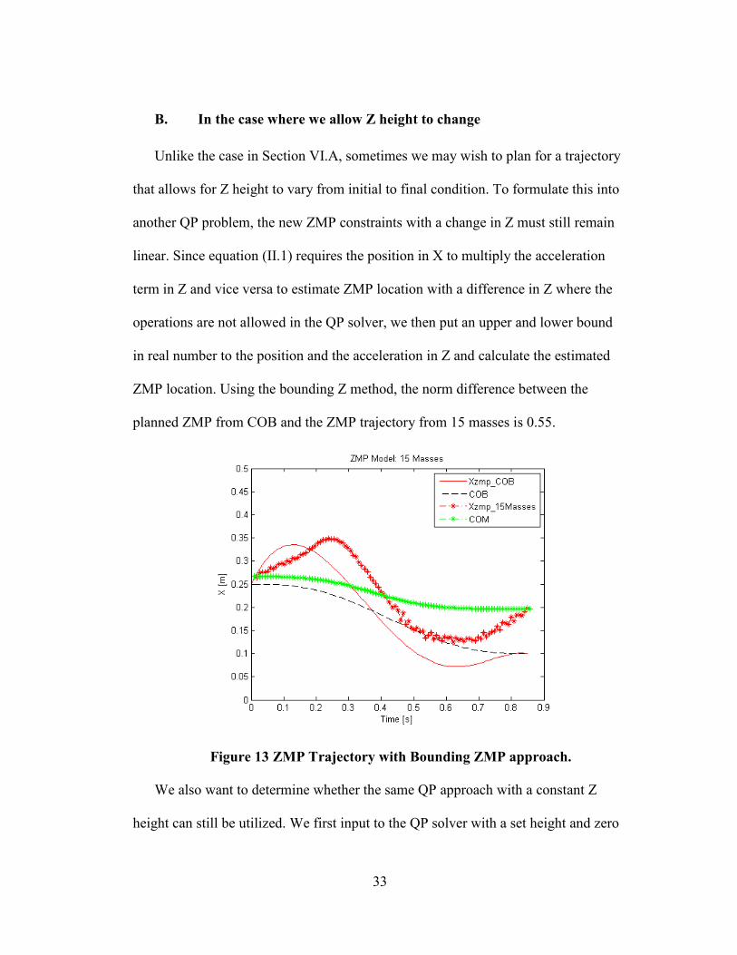
B. In the case where we allow Z height to change

Unlike the case in Section VI.A, sometimes we may wish to plan for a trajectory

that allows for Z height to vary from initial to final condition. To formulate this into

another QP problem, the new ZMP constraints with a change in Z must still remain

linear. Since equation (II.1) requires the position in X to multiply the acceleration

term in Z and vice versa to estimate ZMP location with a difference in Z where the

operations are not allowed in the QP solver, we then put an upper and lower bound

in real number to the position and the acceleration in Z and calculate the estimated

ZMP location. Using the bounding Z method, the norm difference between the

planned ZMP from COB and the ZMP trajectory from 15 masses is 0.55.

Figure 13 ZMP Trajectory with Bounding ZMP approach.

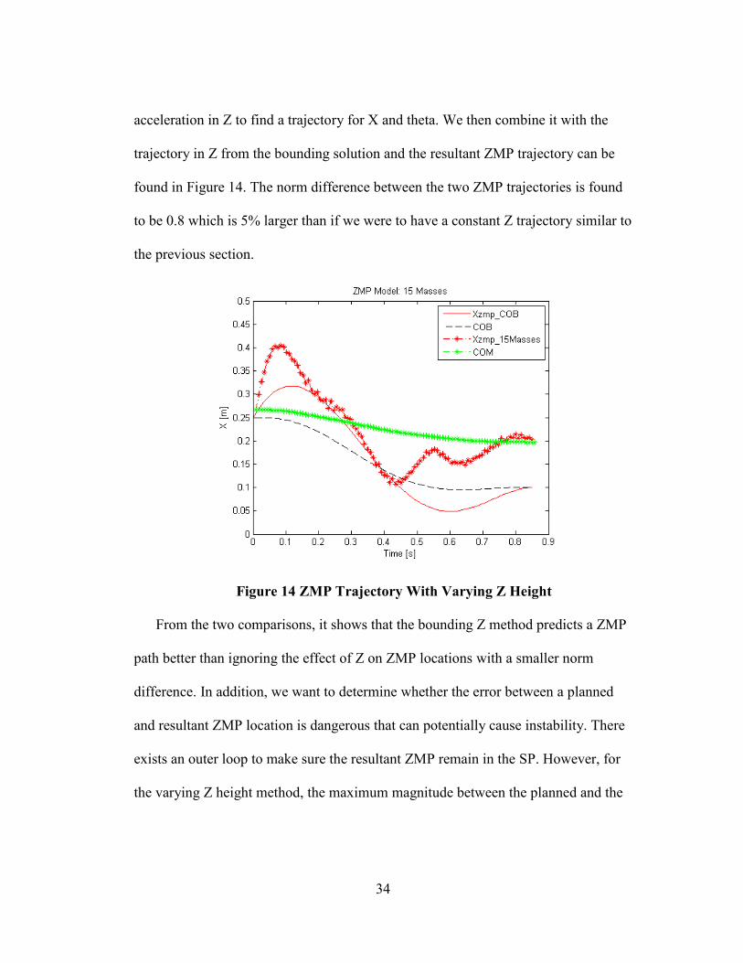
We also want to determine whether the same QP approach with a constant Z

height can still be utilized. We first input to the QP solver with a set height and zero

34

acceleration in Z to find a trajectory for X and theta. We then combine it with the

trajectory in Z from the bounding solution and the resultant ZMP trajectory can be

found in Figure 14. The norm difference between the two ZMP trajectories is found

to be 0.8 which is 5% larger than if we were to have a constant Z trajectory similar to

the previous section.

Figure 14 ZMP Trajectory With Varying Z Height

From the two comparisons, it shows that the bounding Z method predicts a ZMP

path better than ignoring the effect of Z on ZMP locations with a smaller norm

difference. In addition, we want to determine whether the error between a planned

and resultant ZMP location is dangerous that can potentially cause instability. There

exists an outer loop to make sure the resultant ZMP remain in the SP. However, for

the varying Z height method, the maximum magnitude between the planned and the

35

resultant ZMP location has a difference of 0.085 m while the bounding Z method

only has a difference of 0.01 m.

C. Limited Capability (speed and velocity cap)

So far, we have tried to find a minimum time trajectory for the robot without

considering its physical limitation. That is, the robot can be constrained in its joint

position, velocity or acceleration so that the motion plan cannot be executed in real

time. For the test setup, RoboSimian, in fact, is limited in 1

in joint velocity and

acceleration of π

. Hence, given the same solution plan from before for the robot

with a new physical limitation, we want to adjust how the trajectory is being played

back. The most intuitive way to produce an executable trajectory is to apply a

constant scaling for all the to ensure the maximum joint velocity and acceleration

be less or equal to the physical cap. Since the entire COM path stays within the

support polygon, stability will not be violated when the time step is scaled down

constantly. As this is straight forward to implement, we still want to maximize either

the joint velocity or acceleration at each moment in time to achieve the minimum

time trajectory and, of course, to still satisfy the ZMP constraint in the original

problem. Therefore, we loop through each waypoint on the path to find a minimum

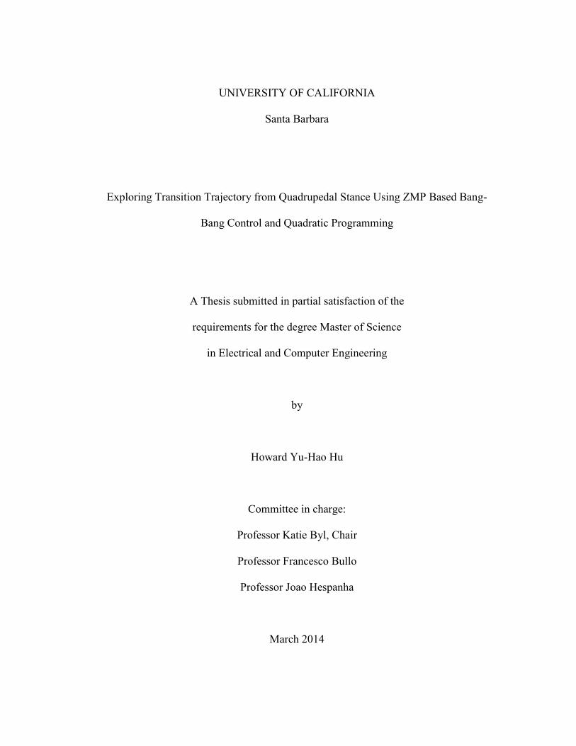
that results in either a max velocity or acceleration. Using the trajectory we found

in Section VI.A with the QP framework, Figure 15 shows the joint velocity

trajectory for the original , constant scaling , and variable approaches for the

same robot motion. Even though the trajectory is slowed down drastically, having

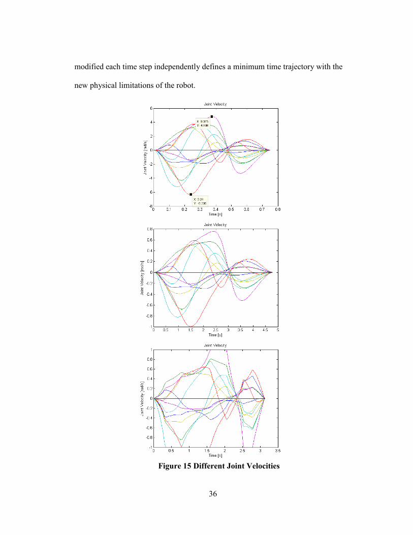
36

modified each time step independently defines a minimum time trajectory with the

new physical limitations of the robot.

Figure 15 Different Joint Velocities

37

The plot on the top shows the planned joint trajectory resulted from QP

solver. The middle applies a constant scale on t from the first plot in order to

satisfy a limited physically capability. The bottom plot maximizes either the

joint velocity or accelerations to minimize the time required for the trajectory.

VII. Conclusion

In this thesis, we look into ways to plan for a transitional motion for a

quadrupedal robot to pitch up its body in preparation to stand in bipedal pose. We

first design a modified bang-bang control to solve for a minimum time problem

using a cart-table model with a stability constraint. Instead of toggling the inputs

between two extreme values of acceleration in the traditional bang-bang control case,

we switch the ZMP location from one edge of the support polygon to another so that

the cart can maintain its stability while applying the greatest acceleration.

We then investigate two quadratic programming problem formulations to solve

for a robot trajectory having front limbs supported against a wall. Such a trajectory

has to satisfy constraints on stability, kinematic reachability and maximum surface

friction. The two methods are tested and compared based on a MATLAB simulation

of RoboSimian. The first approach calculates a planned and constrained ZMP

trajectory from an approximation of COM location based on its COB and solves for

a set of spline coefficients describing the COB trajectory. The second approach, 2-

pass QP, is built on top of the first one with two sub QP problems where it tries to

incorporate the motions of the limbs along with the COB when calculating for ZMP

locations. When we compared the two using Kajita’s cart-table model, the first

method is capable of achieving the transitional motion with a shorter time of 0.75

38

second, while the 2-pass QP approach is slower at 0.8 second but has less error

between the planned and the required ZMP. We also investigate into a trajectory

with an ability to vary Z heights. To do so in QP, we impose an upper and lower

bound on Z when planning for ZMP trajectory and this is a more accurate method

than to blindly assume a constant Z height at all time. Lastly, given a body trajectory,

we simulate a situation when a robot can potentially have a limit on its joint

velocities and accelerations and determine a method to optimize the time needed.

When each waypoint on the trajectory tries to max its velocity and acceleration by

adjusting individual t, the resulted trajectory shortens the time for around 30

percent than if we play the original trajectory with a constant scaled t.

39

VIII. Future Work

Currently, our simulation setup starts and ends with a pose of the robot’s front

limb resting against a wall and all the limbs on the robot are affixed at all time. This

thesis only focuses on pitching up the body while pushing against a wall to obtain a

larger support polygon, but it is not the current scope to plan a trajectory to the initial

state nor is it to self-balance when the body is near the upright position. However,

our ultimate goal in this work is to provide a full package for a robot from starting in

an arbitrary quadrupedal stance to ending in balancing on two limbs. It will be of

interest to apply a similar approach in this thesis to incorporate limbs movement that

may help in performing a transition.

Moreover, the ZMP location stays in the support polygon the throughout the

trajectory. Demonstrating a method to plan for fictitious ZMP location and to

explore an underactuated state of the robot could be an additional method to compare

with the approaches introduced in this thesis.

40

References

[1] M. Vulobratovic et al., “Zero-moment point – Thirty five years of its

life,” in International Journal of Humanoid Robotics, 2004, p. 153-

173.

[2] M. Grant and S. Boyd, “CVX: Matlab software for disciplined convex

programming, version 2.0 beta”, Internet: http://cvxr.com/cvx, 2013.

[3] M. Grant and S. Boyd, “The CVX Users’ guide”, Release 2.0,

Internet: cvxr.com/cvx/doc/CVX.pdf, 2013

[4] K. Byl, “Metastable Legged-Robot Locomotion,” Ph.D. dissertation,

Massachusetts Institution of Technology, Cambridge, 2008

[5] M. Kalakrishnan et al., “Learning, Planning, and Control for

Quadruped Locomotion over Challenging Terrain,” in Inernational

Journal of Robotics Research 30(2), 2011, p. 236 – 258.

[6] Q. Huang et al., “Planning Walking Patterns for a Biped Robot”,in

Proc. IEEE Trans. On Robotics and Automation, 2001, p. 280-289.

[7] S. Kajita et al., “Biped Walking Pattern Generation by using Preview

Control of Zero-moment Point,” in Proc. IEEE ICRA, Taipei, Taiwan,

2003, pp. 1620-1626

[8] S. Sawada et al., “Locomotion Stabilization with Transition between

Biped and Quadruped Walk based on Recognition of Slope,” in Proc.

IEEE Micro-NanoMechatronics and Human Science, 2008, p. 424 –

429.

[9] S. Aoi et al., “Transition from Quadrupedal to Bipedal Locomotion,”

in Proc IEEE International Conference on Intelligent Robots and

Systems, 2005, p. 3419 – 3424.

[10] S. Aoi et al., “Experimental Verification of Gait Transition from

Quadrupedal to Bipedal Locomotion of an Oscillator-driven Biped

Robot,” in Proc IEEE International Conference on Intelligent Robots

and Systems, 2008, p. 1115 – 1120.

41

[11] S. Kudoh et al., “The Dynamic Postural Adjustment with the

Quadratic Programming Method,” in Proc IEEE International

Conference on Intelligent Robots and Systems, 2002, p. 2563 – 2568

[12] S. Collins et al., “The RoboKnee: An Exoskeleton for Enhancing

Strength and Endurance During Walking,” in Proc IEEE

International Conference on Robotics and Automation, 2004, p.2430

– 2435

[13] M. Inaba et al., “Two-Armed Bipedal Robot that can Walk,Roll over

and Stand up,” 1995, p.297 – 302

[14] F. Kanehiro et al., “The First Humanoid Robot that has the Same Size

as a Human and that can Lie down and Get up,” in Proc IEEE

International Conference on Robotics and Automation, 2003, p.1633

– 1639

[15] J. Veneman et al., “Design and Evaluation of the LOPES exoskeleton

robot for Interactive Gait Rehabilitation,” in IEEE transactions on

Neural Systems and Rehabilitation Engineering, Vol.15, No. 3, 2007,

p.379 – 386

[16] A. Gasparetto et al., “Trajectory Planning in Robotics,” Mathematics

in Computer Science, Vol 6, Issue 3, 2012, p. 269 – 279