Exponent Blinding May Not PreventTiming Attacks on RSA

Werner Schindler

Bundesamt fur Sicherheit in der Informationstechnik (BSI)Godesberger Allee 185–189

53175 Bonn, GermanyWerner.Schindler@bsi.bund.de

Abstract. The references [9, 3, 1] treat timing attacks on RSA withCRT and Montgomery’s multiplication algorithm in unprotected imple-mentations. It has been widely believed that exponent blinding wouldprevent any timing attack on RSA. At cost of significantly more timingmeasurements this paper extends the before-mentioned attacks to RSAwith CRT, Montgomery’s multiplication algorithm and exponent blind-ing. Simulation experiments are conducted, which confirm the theoreticalresults. Effective countermeasures exist.

Keywords: Timing attack, RSA, CRT, exponent blinding, Montgomery’s multi-plication algorithm.

1 Introduction

In 1996 Paul Kocher introduced timing analysis [6]. In particular, [6] presentsa timing attack on an unprotected RSA implementation that does not applythe Chinese Remainder Theorem (CRT). Reference [9] introduces a new timingattack on RSA implementations, which apply CRT and Montgomery’s multipli-cation algorithm [8]. This attack was extended to OpenSSL (RSA, CRT, slidingwindow exponentiation algorithm, Montgomery’s multiplication algorithm) [3]and later optimized [1]. Also [5, 9–12] consider timing attacks on RSA imple-mentations that apply Montgomery’s multiplication algorithm. All these attackstarget unprotected RSA implementations.

Besides presenting the first timing attack on RSA (without CRT) [6] pro-poses different countermeasures (Section 10), including exponent blinding wherea random multiple of Euler’s φ function of the modulus is added to the secretexponent. Since then exponent blinding has been widely assumed to be effectiveto prevent (any type of) timing attacks on RSA, at least no successful timingattacks against exponent blinding have been known. The present paper extendsthe timing attack from [9] to RSA implementations, which apply exponent blind-ing, proving that exponent blinding does not always prevent timing attacks onRSA. However, the presence of exponent blinding increases the number of timingmeasurements enormously.

The paper is organized as follows: In Section 2 the targeted implementation isdescribed (RSA with CRT, square & multiply, Montgomery’s multiplication al-gorithm, exponent blinding) while Section 3 contains the theoretical foundationsof our attack. Section 4 specifies the attack and provides experimental results.Moreover, the attack is adjusted to table-based exponentiation algorithms, andeffective countermeasures are proposed.

2 Modular Exponentiation with Montgomery’sMultiplication Algorithm

Modular exponentiations require many hundreds or even thousands of modularmultiplications and squarings. Montgomery’s multiplication algorithms (MM)[8] saves computation time since principally time-consuming modulo operationsand divisions only have to carried out for moduli and divisors, which are powersof 2. This fits perfectly to the hardware architecture of a computer, smart cardor microcontroller.

Definition 1. For a positive integer M > 1 we set ZM := {0, 1, . . . ,M −1}. Asusually, for b ∈ Z the term b(mod M) denotes the smallest nonnegative integer,which is congruent to b modulo M .

Let’s have a brief look at Montgomery’s multiplication algorithm. For an oddmodulus M the integer R := 2t > M is called Montgomery’s constant, andR−1 ∈ ZM denotes its multiplicative inverse modulo M . Moreover, M∗ ∈ ZRsatisfies the integer equation RR−1 −MM∗ = 1.

On input (a, b) Montgomery’s algorithm returns MM(a, b;M) := abR−1( modM). This value is computed with a multiprecision version of Montgomery’smultiplication algorithm, which is adjusted to the particular device. More pre-cisely, let ws denote the word size for the arithmetic operations (typically,ws = 8, 16, 32, 64), which divides the exponent t. Further, r = 2ws, so that inparticular R = rx with v = t/ws (numerical example: (ws, t, v) = (16, 1024, 64)).We express a, b and the term s below in r-adic representation. That is, a =(av−1, ..., a0)r, b = (bv−1, ..., b0)r and s = (sv−1, ..., s0)r. Finally, m∗ = M∗

(mod r). In particular, MM∗ = RR−1 − 1 ≡ −1(modR) and thus m∗ ≡−M−1(mod r)

Algorithm 1. Montgomery’s multiplication algorithm (MM), multiprecision vari-ant

1. Input: a, b ∈ ZM

2. s := 03. For i = 0 to v − 1 do {

u := (s+ aib0)m∗(mod r)s := (s+ aib+ uM)/r

}4. If (s ≥M) then s := s−M [= extra reduction (ER)]

2

5. return (= abR−1(modM) = MM(a, b;M))

After Step 3 s(modM) ≡ abR−1(modM) and s ∈ [0, 2M). The instructions := s − M in Step 4, called ’extra reduction’ (ER), is carried out iff s ∈[M, 2M). This conditional integer subtraction is responsible for timing differ-ences. Whether an ER is necessary does not depend on the chosen multiprecisionvariant but only on the quadruple (a, b,M,R) [9], Remark 1. To determine theprobability distribution of ERs in a modular exponentiation one clearly analysesthe case ws = t, i.e. v = 1.

In the following we assume that Montgomery’s multiplication algorithm at-tains for all pairs (a, b) with 0 ≤ a, b < M (with modulus M and Montgomeryconstant R fixed) only two different execution times, namely

Time (MM(a, b;M)) ∈ {c, c+ cER} for a, b ∈ ZM (M,R fixed). (1)

In the following we will make extensive use of Assumption (1).

Remark 1. (i) Since the divisions and the modular reductions in Step 3 of Al-gorithm 1 can be realized by shifts and masking operations the calculationswithin the for-loop are essentially integer additions and integer multiplicationsor parts thereof, respectively. Usually, log2(M) ≈ log2(R). For known input at-tacks (randomly selected bases) the leading words av−1 and bv−1 are de factoalways non-zero, in particular if ws ≥ 16. Hence one may expect that (1) isfulfilled.(ii) Our timing attack is an adapted chosen input attack, for which in the courseof the attack in many Montgomery multiplications one factor has one or moreleading zero words. For smart cards and microcontrollers one may assume thatthis feature may not not violate (1) since optimizations of rare events (withinthe normal use of the device) seem to be unlikely.(iii) On a PC cryptographic software as OpenSSL, for instance, may processsmall operands (i.e., those with leading zero-words) in Step 3 of Montgomery’salgorithm differently, e.g. because another integer multiplication algorithm isapplied [3, 1]. Such effects, however, may complicate our attack but should notprevent it [3, 1].

Remark 2. In the following we assume that the attacker knows the timing con-stants c and cER. In the best case (from the attacker’s point of view) the attackereither knows both timing constants or is able to determine them precisely witha simulation tool. Otherwise, he has to estimate both values (c.f. Subsection 4.4for details).

Algorithm 2 combines Montgomery’s multiplication algorithm with the square& multiply exponentiation algorithm.

Algorithm 2. Square & multiply with Montgomery’s algorithm (s&m, MM)

Computes y 7→ yd(modM) for d = (dw−1, . . . , 0)2temp := yR := MM(y,R2(modM);M) (Pre-multiplication)

for i=w-1 down to 0 do {

3

temp := MM(temp, temp;M)if (di=1) then temp := MM(temp, yR;M)}

MM(temp, 1;M) (Post-multiplication)

return temp ( = yd(modM) )

As usual, n = p1p2 andR denotes the Montgomery constant while MM(a, b;n) :=abR−1(mod n) stands for the Montgomery multiplication of a and b. The com-putation of v = yd(mod n) is performed in several steps:

Algorithm 3. RSA, CRT, s&m, MM, exponent blinding

1. (a) Set y1 := y(mod p1) and d1 := d(mod (p1 − 1))(b) (Exponent blinding) Generate a random number r1 ∈ {0, 1, . . . , 2eb − 1}

and compute the blinded exponent d1,b := d1+r1φ(p1) = d1+r1(p1−1).

(c) Compute v1 := yd1,b1 (mod p1) with Algorithm 2 (M = p1).

2. (a) Set y2 := y(mod p2) and d2 := d(mod (p2 − 1))(b) (Exponent blinding) Generate a random number r2 ∈ {0, 1, . . . , 2eb − 1}

and compute the blinded exponent d2,b := d2+r2φ(p2) = d2+r2(p2−1).

(c) Compute v2 := yd2,b2 (mod p2) with Algorithm 2 (M = p2).

3. (Recombination) Compute v := yd(mod n) from (v1, v2), e.g. with Garner’salgorithm: v := v1 + p1

(p−11 (mod p2) · (v2 − v1)(mod p2)

)(mod n)

3 Theoretical Background of our Attack

This section contains the theoretical foundations of our attack. The main re-sults of this section are the computation of the mean value and the variance(of the relevant part) of the exponentiation time modulo pi (Subsection 3.1),the development of a distinguisher and the analysis of its relevant properties(Subsection 3.3).

3.1 Exponentiation (mod pi)

In this subsection we investigate the stochastic timing behaviour of the expo-nentiations modulo p1 and modulo p2. As in Algorithm 3 the blinding factor riis an eb-bit number, i.e. ri ∈ {0, . . . , 2eb − 1} for i = 1, 2.

Definition 2. Random variables are denoted by capital letters, and realizations(i.e., values taken on) of these random variables are denoted with the correspond-ing small letter. The abbreviation ’iid’ stands for ’independent and identicallydistributed’. For a random variable Y the terms E(Y ), E2(Y ) and Var(Y ) de-note its expectation (mean), its second moment and its variance, respectively.The term Y ∼ N(µ, σ2) means that the random variable N is normally distrib-uted with mean µ and variance σ2. The cumulative distribution of the standardnormal distribution N(0, 1) is given by Φ(x) := (2π)−1/2

∫ x−∞ e−t

2/2 dt.

4

We interpret the measured execution times as realizations of random variables.In this subsection we focus on Step 1(c) and Step 2(c) of Algorithm 3. Moreprecisely, we consider the for-loop in Algorithm 2 with M = pi for i = 1, 2. Thedistinguisher (Subsect. 3.3) and the attack (Sect. 4) consider input values of theform y = uR−1(mod n). A simple calculation shows that the pre-multiplicationstep in Algorithm 2 transforms the input value y to yR,i := u(modpi) ([9],Sect. 3, after formula (5)). Consequently, we interpret the execution time of thefor loop in Algorithm 2 as a realization of a random variable Zi(u). With thisnotation

Zi(u) := (Qi +Mi)c+Xi cER (2)

expresses the random computation time for the exponentiation ( mod pi) in termsof the random variables Qi, Mi and Xi. The random variables Qi and Mi de-note the random number of squarings and multiplications within the for loopin Step i(c) while Xi quantifies the number of extra reductions (ERs) in thesesquarings and multiplications. Unfortunately, the random variables Qi, Mi andXi are not independent.

The main goal of this subsection is to calculate E(Zi(u)) and Var(Zi(u)). Bydefinition

E (Zvi (u)) =∑qj

∑mk

∑xr

P (Qi = qi,Mi = mk, Xi = xr) ((qi +mk)c+ xr cER) =

∑qj

P (Qi = qj)∑mk

P (Mi = mk | Qi = qj)∑xr

P (Xi = xr | Qi = qj ,Mi = mk) ×

× ((qi +mk)c+ xr cER)v. (3)

Clearly, xr ∈ {0, . . . , qj +mk}, mk ∈ {0, . . . , qj} and qj ∈ {k− 1, . . . , k+ eb− 1}.Lemma 1 collects some facts, which will be needed in the following. Recall thatpi < R.

Lemma 1. As in Section 2 the term yi stands for y(mod pi).(i) For y := uR−1(modn) the MM-transformed basis for the exponentiation(mod pi) equals u′i := u(mod pi).

(ii) If di,b is a k′i-bit integer the computation of ydi,bi (mod pi) needs qi := k′i − 1

squarings and mi := ham(di,b)− 1 multiplications.(iii) The (conditional) random variable (Xi | Qi = qi,Mi = mi) cER quantifiesthe overall random execution time for all extra reductions if Qi = qi and Mi =mi. Let

pi∗ :=pi3R

, pi(u′) :=u′i2pi

, covi,MS(u′i) := 2p3i(u′)pi∗ − pi(u′)pi∗ , (4)

covi,SM(u′i) :=

9

5pi(u′)p

2i∗ − pi(u′)pi∗ , covi,SS :=

27

7p4i∗ − p2i∗ . (5)

The random variable (Xi | Qi = qi,Mi = mi) is normally distributed withexpectation and variance

E(Xi | Qi = qi,Mi = mi) = qipi∗ +mipi(u′) and (6)

5

Var(Xi | Qi = qi,Mi = mi) = qipi∗(1− pi∗) +mipi(u′)(1− pi(u′)) +

2micovi,SM(u′i) + 2(mi − 1)covi,MS(u′

i) + 2(qi −mi)covi,SS (7)

(iv) The random variable (Mi | Qi = qi) quantifies the random number of multi-plications if Qi = qi. It is approximately N(qi/2, qi/4)-distributed. In particular,E(M2

i | Qi = qi) = 14 (qi + q2i ).

Proof. The assertions (i) and (ii) are obvious. Altogether, qi +mi Montgomeryoperations (squarings and multiplications) are carried out. Since gcd(di,b, p−1) =1 the last binary digit of di,b is 1. Hence mi times a multiplication follows asquaring, mi−1 times a squaring follows a multiplication, and q+mi−1−mi−(mi−1) = q−mi times a squaring follows a squaring. Formulae (6) and (7) havebeen proved in Theorem 2 in [9]. In (iv) we assume that (apart from the mostsignificant bit) the digits of the blinded exponent di,b independently assume thevalues 0 and 1 with probability 1/2.

For v = 1 the evaluation of (3) quite easy. As in Lemma 1 we define u′ :=u(mod pi) to simplify the notation. In particular, u′ ∈ Zpi . In fact, by Lemma 1we have Xi = Xi(u

′) whereas Qi and Mi do not depend on u′.

E (Zi(u)) =∑qj

P (Qi = qj)∑mk

P (Mi = mk | Qi = qj)((qi +mk) c+

(qjpi∗ +mkpi(u′)

)cER

)=

∑qj

P (Qi = qj)((qj +

qj2

)c+

(qjpi∗ +

qj2pi(u′)

)cER

)=

E(Qi)

(3

2c+

(pi∗ +

1

2pi(u′)

)cER

). (8)

Careful calculations yield

E(Z2i (u)

)=∑

qj

P (Qi = qj)∑mk

P (Mi = mk | Qi = qj)∑xr

P (Xi = xr | Qi = qj ,Mi = mk) ×

×((qi +mk)2c2 + 2(qj +mk)xrc cER +x2rcER

2)

=∑qj

P (Qi = qj)∑mk

P (Mi = mk | Qi = qj) ×

×(

(qj +mk)2c2 + 2(qj +mk)E (Xi | Qi = qj ,Mi = mk) c cER +(

Var (Xi | Qi = qj ,Mi = mk) + E2 (Xi | Qi = qj ,Mi = mk))cER

2)

(9)

Substituting (6) and (7) into (9) yields∑qj

P (Qi = qj)∑mk

P (Mi = mk | Qi = qj) ×

6

×(

(qj +mk)2c2 + 2(qj +mk)(qjpi∗ +mkpi(u′))c cER

+(qjpi∗(1− pi∗) +mkpi(u′)(1− pi(u′)) + 2(mk − 1)(2p3i(u′)pi∗ − pi(u′)pi∗)

+2mk(9

5pi(u′)p

2i∗ − pi(u′)pi∗) + 2(qj −mk)(

27

7p4i∗ − p2i∗)

+(qjpi∗ +mkpi(u′))2)cER

2)

(10)

By Lemma 1(iv), and since∑qjP (Qi = qj)q

vj = E(Qvi ) we finally obtain

E(Z2i (u)

)= E(Q2

i )

(3

2c+ (pi∗ +

1

2pi(u′)) cER

)2

+E(Qi)(1

4c2 +

1

2pi(u′)c cER +

(pi∗(1− pi∗) +

1

2pi(u′)(1− pi(u′))

+2p3i(u′)pi∗ +9

5pi(u′)p

2i∗ − 2pi(u′)pi∗ +

27

7p4i∗ − p2i∗ +

1

4pi(u′))cER

2)

−2(2p3i(u′)pi∗ − 2pi(u′)pi∗)cER2 (11)

Theorem 1. Combining the previous results we obtain

E (Zi(u)) = E(Qi)

(3

2c+

(pi∗ +

1

2pi(u′)

)cER

)(12)

and

Var (Zi(u)) = Var(Qi)

(3

2c+ (pi∗ +

1

2pi(u′)) cER

)2

+E(Qi)(1

4c2 +

1

2pi(u′)c cER +

(pi∗(1− pi∗) +

1

2pi(u′)(1− pi(u′))

+2p3i(u′)pi∗ +9

5pi(u′)p

2i∗ − 2pi(u′)pi∗ +

27

7p4i∗ − p2i∗ +

1

4pi(u′))cER

2)

−2(2p3i(u′)pi∗ − 2pi(u′)pi∗)cER2 . (13)

Proof. Equation (12) equals (8), and (13) follows immediately from (11) and (8).

Lemma 2 provides explicit expressions for the terms E(Qi) and Var(Qi). Notethat pi < 2k ≤ R.

Lemma 2. Let pi be a k-bit number, and let γi := pi/2k.

(i) Unless eb is artificially small in good approximation

E(Qi) = (k − 1) + eb− 1

γi(14)

Var(Qi) =3

γi− 1

γ2i(15)

(ii) In particular, E(Qi) is monotonously increasing in γi and assumes values in(k− 1 + eb− 2, k− 1 + eb− 1). The variance Var(Qi) assumes values in (2, 2.25].The maximum value 2.25 is taken on for γi = 2/3. If 2k = R (typical case) thenγi = 3pi∗.

7

Proof. A k-bit integer needs q = k−1 squarings. Unless the parameter eb is verysmall, in good approximation

E(Qvi ) =

eb∑j=0

(k − 1 + j)v2−eb∣∣{r : 2k−1+j ≤ di + r(pi − 1) < 2k+j}

∣∣≈

eb∑j=0

(k − 1 + j)v2−eb∣∣{r : 2k+j−1 ≤ rpi < 2k+j}

∣∣≈eb−1∑j=0

(k − 1 + j)v2−eb(∣∣{r : rpi < 2k+j}

∣∣− ∣∣{r : rpi < 2k+j−1}∣∣)+

(k − 1 + eb)v2−eb(2eb −

∣∣{r : rpi < 2k+eb−1}∣∣ ) .

For ’large’ indices j the approximation error in the second line is negligible,and for small indices j the summands have only negligible contribution to thesum. Hence the approximation error is practically irrelevant. (For the sake ofcompleteness we point out that if di is smaller than 2k−1 blinded exponents mayoccur, which are shorter than k bits. The probability is yet negligible.) With|{r : rpi < 2k+j}| ≈ 2k+j/pi = 2j/γi the above formula simplifies to

E(Qvi ) ≈eb−1∑j=0

(k − 1 + j)v2−eb2j−1

γi+ (k − 1 + eb)v2−eb

(2eb − 2eb−1

γi

)

=2−eb

γi

eb−1∑j=0

(k − 1 + j)v2j−1 + (k − 1 + eb)v(

1− 1

2γi

).

For t 6= 0, 1 elementary calculus yields

eb−1∑j=0

tj−1 = t−1 +teb−1 − 1

t− 1,

eb−1∑j=0

jtj−1 =d

dt

eb−1∑j=1

tj =d

dt

(teb − 1

t− 1− 1

)=

(eb− 1)teb − ebteb−1 + 1

(t− 1)2

eb−1∑j=0

j(j − 1)tj−1 = t · d2

dt2

eb−1∑j=2

tj = t · d2

dt2

(teb − 1

t− 1− t− 1

)

=

((eb− 2)(eb− 1)t2 − 2eb(eb− 2)t+ eb(eb− 1)

)teb−1 − 2t

(t− 1)3

For t = 2 the first two formulae yield

E(Qi) ≈2−eb

γi

((k − 1)

(2eb−1 − 1

2

)+ ((eb− 1)2eb − eb2eb−1 + 1)

)+ (k − 1 + eb)

(1− 1

2γ

)≈ (k − 1)

1

2γi+

1

2γi(eb− 2 + 2−eb+1) + (k − 1)

(1− 1

2γi

)+ eb

(1− 1

2γi

)

8

Neglecting the term 2−eb+1/2γi and simplifying the remaing terms yields(14). Using the above formulae we obtain

Var(Qi) = Var(Qi − (k − 1)) = E((Qi − (k − 1))2

)− E2 (Qi − (k − 1))

=2−eb

γi

eb−1∑j=0

j2j−1 +

eb−1∑j=0

j(j − 1)2j−1

+ eb2(

1− 1

2γi

)

Substituting the two sums by the above formula (for t = 2) and cancellingnegligible terms (as for v = 1) yields (15). The assertions of Lemma 2(ii) can beverified with methods from elementary calculus.

Remark 3. (i) Setting Var(Qi) = 0 and E(Qi) = k − 1 Theorem 1 gives theformulae for non-blinded implementations.(ii) Numerical experiments verify that (15) approximates Var(Qi) very well.

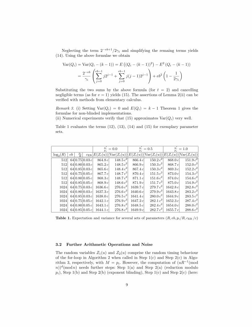
Table 1 evaluates the terms (12), (13), (14) and (15) for exemplary parametersets.

u′

pi= 0.0 u′

pi= 0.5 u′

pi= 1.0

log2(R) eb piR

cER E(Zi(u)) Var(Zi(u)) E(Zi(u)) Var(Zi(u)) E(Zi(u)) Var(Zi(u))

512 64 0.75 0.03 c 864.8 c 148.5 c2 866.4 c 150.2 c2 868.0 c 151.9 c2

512 64 0.80 0.03 c 865.2 c 148.5 c2 866.9 c 150.3 c2 868.7 c 152.0 c2

512 64 0.85 0.03 c 865.6 c 148.4 c2 867.4 c 150.3 c2 869.3 c 152.2 c2

512 64 0.75 0.05 c 867.7 c 148.7 c2 870.4 c 151.5 c2 873.0 c 154.3 c2

512 64 0.80 0.05 c 868.3 c 148.7 c2 871.1 c 151.6 c2 874.0 c 154.6 c2

512 64 0.85 0.05 c 868.9 c 148.6 c2 871.9 c 151.7 c2 875.0 c 154.9 c2

1024 64 0.75 0.03 c 1636.6 c 276.6 c2 1639.7 c 279.7 c2 1642.8 c 282.8 c2

1024 64 0.80 0.03 c 1637.3 c 276.6 c2 1640.6 c 279.9 c2 1643.8 c 283.2 c2

1024 64 0.85 0.03 c 1638.0 c 276.5 c2 1641.4 c 280.0 c2 1644.9 c 283.5 c2

1024 64 0.75 0.05 c 1642.1 c 276.9 c2 1647.2 c 282.1 c2 1652.3 c 287.4 c2

1024 64 0.80 0.05 c 1643.1 c 276.8 c2 1648.5 c 282.4 c2 1654.0 c 288.0 c2

1024 64 0.85 0.05 c 1644.1 c 276.8 c2 1649.9 c 282.7 c2 1655.7 c 288.6 c2

Table 1. Expectation and variance for several sets of parameters (R, eb, pi/R, cER /c)

3.2 Further Arithmetic Operations and Noise

The random variables Z1(u) and Z2(u) comprise the random timing behaviourof the for-loop in Algorithm 2 when called in Step 1(c) and Step 2(c) in Algo-rithm 3, respectively, with M = pi. However, the computation of (uR−1(modn))d(modn) needs further steps: Step 1(a) and Step 2(a) (reduction modulopi), Step 1(b) and Step 2(b) (exponent blinding), Step 1(c) and Step 2(c) (here:

9

pre-multiplication and post-multiplication of Algorithm 2), Step 3 (recombina-tion), time for input and output etc. In analogy to Subsection 3.1 we view therequired overall execution time for the before-mentioned steps as a realizationof a random variable Z3(u).

It seems reasonable to assume that the time for input and output of data,for recombination and blinding as well as the reduction (mod pi) in Step 1(a)and Step 2(a) of Algorithm 3 do not (or at most weakly) depend on u. Thepostprocessing step in Algorithm 2 never needs an ER. (By [13], Theorem 1, inAlgorithm 1 after Step 3 we have s ≤M + temp · r−v < M + 1, and thus s ≤M .If s = M then temp = 0 after the extra reduction, which only can happen if u isa multiple of M = pi but then yR = uR−1R ≡ 0( mod pi), and Algorithm 2 doesnot need any extra reduction at all.) In the pre-multiplication in Algorithm 2 anER may occur or not. Altogether, we may assume

E(Z3(u)) ≈ z3 for all u ∈ Zn and (16)

Var(Z3(u))� Var(Z1(u)),Var(Z2(u)) (17)

In the following we assume E(Z3(u)) = z3 for all u and view the centeredrandom variable Z3(u) − z3 as part of the noise. This and possibly additionalnoise, e.g. caused by measurement errors, is captured by the random variableNe. If Var(Ne) = σ2

N > 0 we assume Ne ∼ N(µN , σ2N ). Of course, σ2

N = 0 means’no noise’, and Ne = z3 with probability 1.

3.3 The Distinguisher

In this subsection we derive a distinguisher, which will be the core of our attack(to be developed in Section 4). The overall random execution time for input uis described by the random variable

Z(u) = Z1(u) + Z2(u) + z3 +Ne . (18)

In the following we assume

0 < u1 < u2 < n and u2 − u1 � p1, p2 . (19)

Theorem 1 implies

E (Z(u2)− Z(u1)) = E (Z1(u2)− Z1(u1)) + E (Z2(u2)− Z2(u1)) (20)

=1

2

2∑i=1

E(Qi)(pi(u′

(2)) − pi(u′

(1))

)cER with u′(j) = uj(mod pi)

As in [9] we distinguish between three cases:Case A: The interval {u1 + 1, . . . , u2} does not contain a multiple of p1 or p2.Case B: The interval {u1 + 1, . . . , u2} contains a multiple of ps but not of p3−s.Case C: The interval {u1 + 1, . . . , u2} contains a multiple of p1 and p2.

10

Let’s have a closer look at (20). By (4)

pi(u′(2)

) − pi(u′(1)

)

{= u2−u1

2R cER ≈ 0 Case A, Case B (for i 6= s)≈ − pi

2R cER Case B (for i = s), Case C(21)

Further,

E(Qi) = ki + eb− 1− γ−1i = 2dlog2(pi)e + eb− 1− 2ki

pi

= log2(R) + (dlog2(pi)e − log2(R)) + eb− 1− R

pi· 2ki

R(22)

where dxe denotes the smallest integer ≥ x. Since during the attack the primesp1 and p2 are unknown we use the approximation

p1, p2 ≈√n and set β :=

√n

R. (23)

With approximation (23) formula (22) simplifies to

E(Qi) ≈ log2(R) + eb− 1− β−1 if√

0.5 < β < 1 , and similarly (24)

Var(Qi) ≈ 3β−1 − β−2 if√

0.5 < β < 1 (25)

since ki = dlog2(pi)e = log2(R) then. Finally (21) and (24) imply

E (Z(u2)− Z(u1)) ≈

0 in Case A− 1

4 ((log2(R) + eb− 1)β − 1) cER in Case B− 1

2 ((log2(R) + eb− 1)β − 1) cER in Case C(26)

In the following we focus on the case√

0.5 < β < 1, which is the most relevantcase since then 0.5R2 < n < R2, i.e. n is a 2 log2(R) bit modulus and, conse-quently, p1 and p2 are log2(R)-bit numbers. We point out that the case β <

√0.5

can be treated analogously. In (24) and (25) the parameter β−1i then should bebetter replaced by β−1i 2dlog2(pi)e−log2(R). However, the ’correction factor’ maynot be unambiguous, which might lead to some inaccuracy in the formulae, fi-nally implying a slight loss of attacking efficiency.

From (18) we obtain

Var (Z(u2)− Z(u1)) =

2∑j=1

(2∑i=1

Var (Zi(uj)) + Var(Ne,j)

)(27)

For given R, eb, c, cER, u the variance Var(Zi(u)) is nearly independent of pi/Rand increases somewhat when the ratio u/pi increases (c.f. Table 1). Since thetrue values p1/R and p2/R are unknown during the attack we approximate (27)by

Var (Z(u2)− Z(u1)) ≈ 4varβ;max + 2σ2N (28)

11

Here ’varβ;max’ suggestively stands for the term (13) with βR in place of pi andu′, i.e. we replace the probabilities pi∗ and pi(u′) by β/3 and β/2, respectively. Wepoint out that variance (27) has no direct influence on the decision strategy of ourattack but determines the needed sample size. Usually, (28) should overestimate(27) somewhat. Moreover, decision errors can be detected and corrected (c.f.Section 4, ’confirmed intervals’). So we should be on the safe side anyway. Forfixed pi the mean E(Zi(u)) increases monotonically in u/pi (c.f. (12)). In fact,our attack exploits these differences.

On basis of execution times for input values (bases) y = uiR−1(mod n) (i =

1, 2) the attacker has to decide hundreds of times whether some interval {u1 +1, . . . , u2} contains a multiple of p1 or p2. By (26) the value

decbound := −1

8((log2(R) + eb− 1)β − 1) cER (29)

is a natural decision boundary. In fact, for given u1 < u2 and yi := (u2R−1( mod

n) this suggests the following decision rule:

Decide for Case A iff Time(yd2(mod n))− Time(yd1(mod n)) > decbound ,

and for (Case B or Case C) else. (30)

(Note that we do not need to distinguish between Case B and Case C.) HereTime(ydi (mod n)) denotes the execution time for input value yi, which of coursedepends on the blinding factors for the modular exponentiation (mod p1) and(modp2). However, the variance Var(Z(u2) − Z(u1)) is too large for reliabledecisions. Thus we consider N iid random variables Z[1](u), . . . , Z[N ](u) in placeof Z(u), which are distributed as Z(u) (corresponding to N exponentiations withinput value y = uR−1( mod n)). Unlike for decision strategy (30) we evaluate theaverage timing difference from N pairs of timing measurements (c.f. Sect. 4). ForNτ the inequality√√√√√Var

1

Nτ

Nτ∑j=1

(Z[j](u2)− Z[j](u1)

) ≈√

4varβ;max + 2σ2N

Nτ

≤ |decbound− 0|τ

implies

Nτ ≥τ2(4varβ;max + 2σ2

N )

|decbound|2=

64τ2(4varβ;max + 2σ2N )

((log2(R) + eb− 1)β − 1)2cER

2. (31)

Applying the above decision strategy (30) to N ≥ Nτ pairs of timing differencesthe Central Limit Theorem then implies

Prob(wrong decision) ≤ Φ(−τ) . (32)

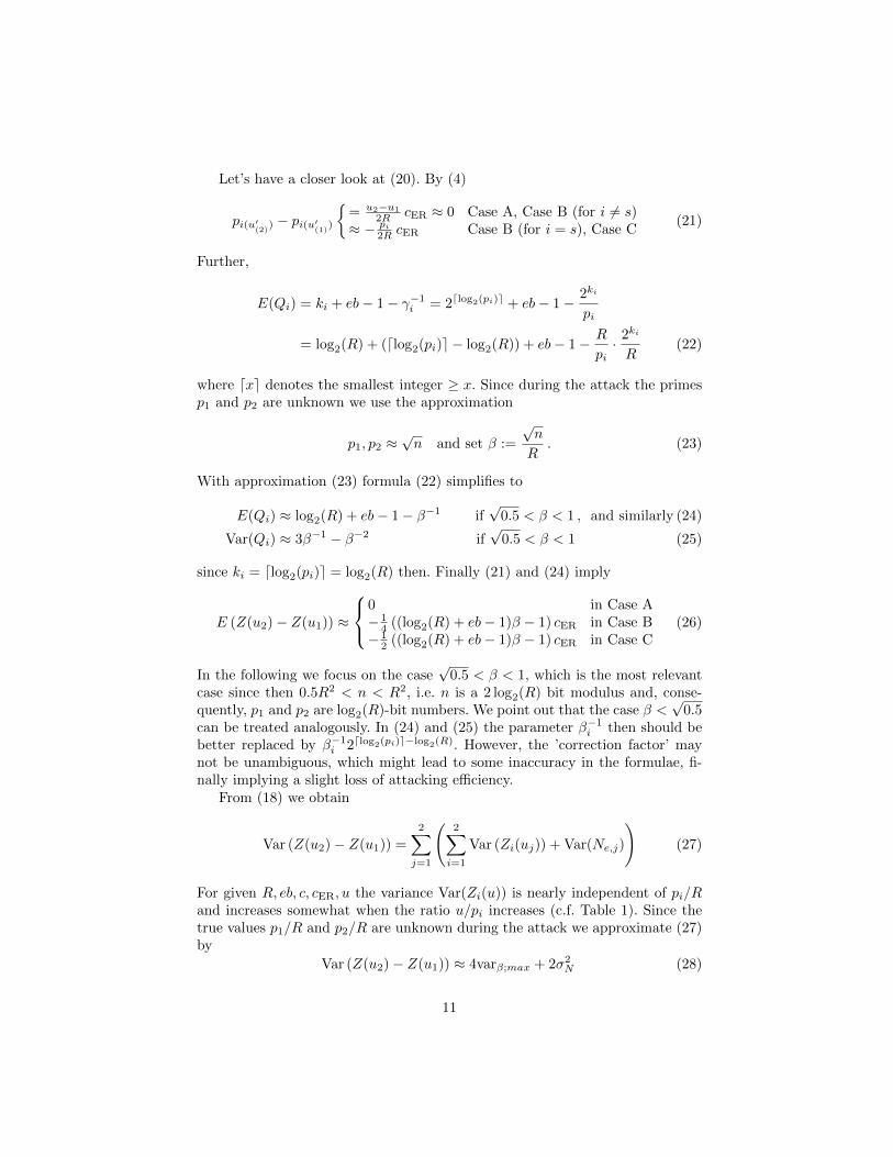
Table 2 evaluates (31) for several parameter sets with σ2N = 0. If σ2

N = α(2varβ;max)the sample size Nτ increases by factor (1 + α).

12

log2(R) eb cER β =√nR

N2.5 N2.7 β =√nR

N2.5 N2.7

512 64 0.03 c 0.75 1458 1701 0.85 1137 1326512 64 0.05 c 0.75 533 622 0.85 417 486

1024 64 0.03 c 0.75 758 885 0.85 592 6901024 64 0.05 c 0.75 277 324 0.85 217 253

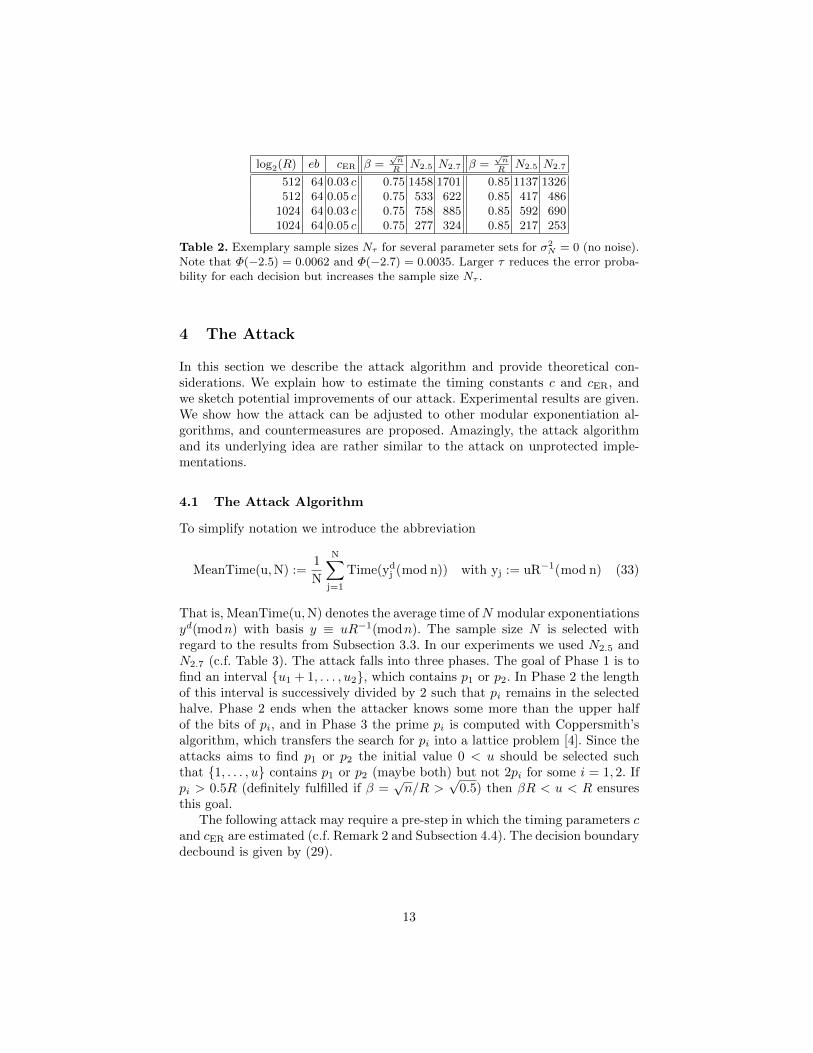
Table 2. Exemplary sample sizes Nτ for several parameter sets for σ2N = 0 (no noise).

Note that Φ(−2.5) = 0.0062 and Φ(−2.7) = 0.0035. Larger τ reduces the error proba-bility for each decision but increases the sample size Nτ .

4 The Attack

In this section we describe the attack algorithm and provide theoretical con-siderations. We explain how to estimate the timing constants c and cER, andwe sketch potential improvements of our attack. Experimental results are given.We show how the attack can be adjusted to other modular exponentiation al-gorithms, and countermeasures are proposed. Amazingly, the attack algorithmand its underlying idea are rather similar to the attack on unprotected imple-mentations.

4.1 The Attack Algorithm

To simplify notation we introduce the abbreviation

MeanTime(u,N) :=1

N

N∑j=1

Time(ydj (mod n)) with yj := uR−1(mod n) (33)

That is, MeanTime(u,N) denotes the average time ofN modular exponentiationsyd(modn) with basis y ≡ uR−1(modn). The sample size N is selected withregard to the results from Subsection 3.3. In our experiments we used N2.5 andN2.7 (c.f. Table 3). The attack falls into three phases. The goal of Phase 1 is tofind an interval {u1 + 1, . . . , u2}, which contains p1 or p2. In Phase 2 the lengthof this interval is successively divided by 2 such that pi remains in the selectedhalve. Phase 2 ends when the attacker knows some more than the upper halfof the bits of pi, and in Phase 3 the prime pi is computed with Coppersmith’salgorithm, which transfers the search for pi into a lattice problem [4]. Since theattacks aims to find p1 or p2 the initial value 0 < u should be selected suchthat {1, . . . , u} contains p1 or p2 (maybe both) but not 2pi for some i = 1, 2. Ifpi > 0.5R (definitely fulfilled if β =

√n/R >

√0.5) then βR < u < R ensures

this goal.The following attack may require a pre-step in which the timing parameters c

and cER are estimated (c.f. Remark 2 and Subsection 4.4). The decision boundarydecbound is given by (29).

13

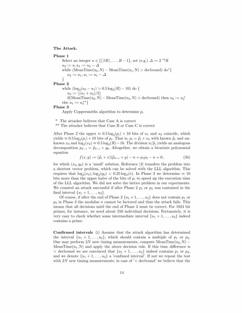
The Attack.

Phase 1Select an integer u ∈ {dβRe, . . . , R− 1}, set (e.g.) ∆ := 2−6Ru2 := u, u1 := u2 −∆while (MeanTime(u2,N)−MeanTime(u1,N) > decbound) do∗{

u2 := u1, u1 := u1 −∆}

Phase 2while (log2(u2 − u1) > 0.5 log2(R)− 10) do {

u3 := b(u1 + u2)/2cif(MeanTime(u2,N)−MeanTime(u3,N) > decbound) then u2 := u ∗3

else u1 := u ∗∗3 }Phase 3

Apply Coppersmiths algorithm to determine pi

* The attacker believes that Case A is correct** The attacker believes that Case B or Case C is correct

After Phase 2 the upper ≈ 0.5 log2(pi) + 10 bits of u1 and u2 coincide, whichyields ≈ 0.5 log2(pi) + 10 bits of pi. That is, pi = pi + x0 with known pi and un-known x0 and log2(x0) ≈ 0.5 log2(R)−10. The division n/pi yields an analogousdecomposition p3−i = p3−i + y0. Altogether, we obtain a bivariate polynomialequation

f(x, y) := (pi + x)(p3−i + y)− n = p1p2 − n = 0 , (34)

for which (x0, y0) is a ’small’ solution. Reference [4] transfers the problem intoa shortest vector problem, which can be solved with the LLL algorithm. Thisrequires that log2(x0), log2(y0) < 0.25 log2(n). In Phase 2 we determine ≈ 10bits more than the upper halve of the bits of pi to speed up the execution timeof the LLL algorithm. We did not solve the lattice problem in our experiments.We counted an attack successful if after Phase 2 p1 or p2 was contained in thefinal interval {u1 + 1, . . . , u2}.

Of course, if after the end of Phase 2 {u1 + 1, . . . , u2} does not contain p1 orp2 in Phase 3 the modulus n cannot be factored and thus the attack fails. Thismeans that all decisions until the end of Phase 2 must be correct. For 1024 bitprimes, for instance, we need about 550 individual decisions. Fortunately, it isvery easy to check whether some intermediate interval {u1 + 1, . . . , u2} indeedcontains a prime.

Confirmed intervals (i) Assume that the attack algorithm has determinedthe interval {u1 + 1, . . . , u2}, which should contain a multiple of p1 or p2.One may perform 2N new timing measurements, compute MeanTime(u2,N) −MeanTime(u1,N) and apply the above decision rule. If this time difference is< decbound we are convinced that {u1 + 1, . . . , u2} indeed contains p1 or p2,and we denote {u1 + 1, . . . , u2} a ’confimed interval’. If not we repeat the testwith 2N new timing measurements: in case of ’< decbound’ we believe that the

14

first test result was false, and {u1 + 1, . . . , u2} is the new confirmed interval. Ifagain ’> decbound’ we believe that an earlier decision was wrong and restartthe attack at the preceding confirmed interval. Confirmed intervals should beestablished after con decisions. The value con should be selected with regard tothe probability for a wrong individual decision. It is reasonable to establish thefirst confirmed interval after Phase 1.(ii) In the unprotected case the determined interval {u1 + 1, . . . , u2} must bevalidated for neighboured integers, e.g. for u1 + 1 and u2 − 1, u1 + 2 and u2 − 2[9]. In the presence of exponent blinding we may use u1 and u2.(iii) Of course, an erroneously confirmed interval will let the attack fail. Thisprobability can be reduced e.g. by applying a ’majority of three’ decision rulewhere the ’original’ interval {u1 + 1, . . . , u2} (determined by our attack algo-rithm) unlike in (i) does not count. Alternatively, the algorithm might jumpback to the last but one confirmed interval if the preceding confirmed intervalturns out to be wrong with high probability.

Remark 4. Phase 1 and Phase 2 of our attack require roughly ≈ (0.5 log2(R) +30)Nτ timing measurements plus the timing measurements that are necessaryto establish confirmed intervals and to correct preceding wrong decisions, if nec-essary.

Remark 5. [Scaling] Assume eb� log2(R), which is typical.(i) By (29) and (13) doubling the length of the prime factors p1 and p2 roughlydoubles decbound (and thus the intervals [decbound, 0] and [2decbound,decbound],c.f. (26) and (29)) and varβ;max. If σ2

N ≈ 0 by (31) Nτ decreases to approximately50%. On the other hand the attack needs about twice as many individual in-dividual decisions (c.f. Remark 4). This points to the surprising fact that theoverall number of timing measurements per attack is to a large extent indepen-dent of the modulus length if σ2

N ≈ 0.(ii) Similarly, halving cER halves decbound but leaves varβ;max nearly unchanged.If σ2

N ≈ 0 by (31) the attack then requires about 4 times as many timing measure-ments. More precisely, decbound depends linearly on cER (29). For realistic ratioscER /c in (13) the E(Qi)(. . .)-term, and within the bracket the first summanddominates. Consequently, (31) implies that the number of timing measurementsincreases roughly like (cER /c)

−2.(iii) Our simulation experiments confirm both assertions (c.f. Table 3).

Remark 6. As its predecessors in [9, 3, 1] our attack and its variants for table-based exponentiation algorithms (c.f. Subsection 4.5) are adaptive chosen inputattacks. We point out that the attack would also work for input values (uj +x)R−1(modn) with |x| � n1/4 in place of the input values ujR

−1(modn).This property allows to meet possible minor restrictions on the input values(e.g. some set bits), which might be demanded by the targeted RSA application.

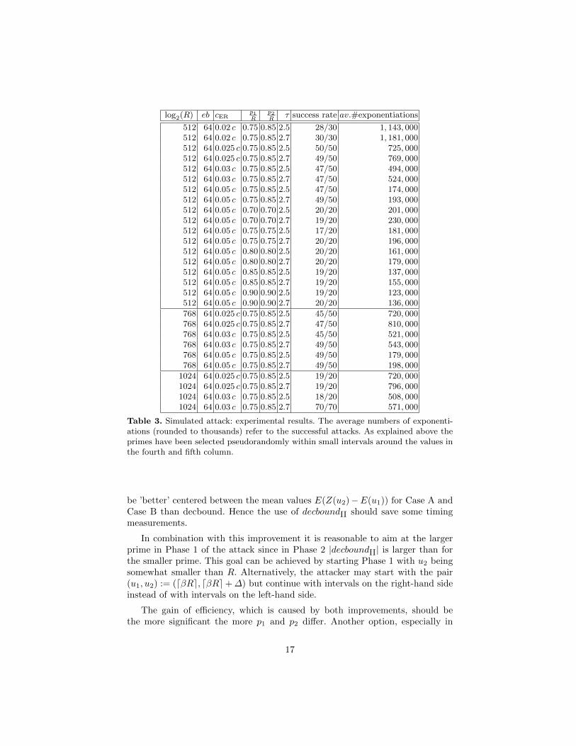
4.2 Experimental Results

In this subsection we present experimental results. As already pointed out inSection 2 it only depends on the quadruple (a, b,M,R) but not on any fea-

15

tures of the implementation whether MM(a, b;M) requires an extra reduction.This property allows to simulate the modular exponentiations yd(modn) andto count the number of extra reductions, which finally corresponds to an attackunder perfect timing measurements and with E(Z3(u)) = z3, Var(Z3(u)) = 0,i.e. Z3(u) ≡ z3 for all 0 < u < n, which is an idealization of (16) and (17).Consequently, also in the absence of noise in real-life experiments the number oftiming measurements thus should be somewhat larger than for our simulationexperiments. The impact of noise was quantified in Subsection 3.3.

In our experiments we selected the primes p1 and p2 pseudorandomly. Thetable entry pi/R = 0.75, for instance, means that pi has been selected pseudo-randomly in the interval [0.75−0.025, 0.75+0.025]R. The secret exponent d wascomputed according to the public exponent e = 216 + 1. Table 3 provides exper-imental results for several sets of parameters. In our experiments we assumedσ2N = 0. We calculated Nτ with formula (31), which also allows to extrapolate

the number of timing measurements for any noise level. Table 3 confirms theconsiderations from Remark 5. Several experiments with p1/R ≈ p2/R wereconducted, which verify that the attack becomes the more efficient the largerthese ratios are. The reason is that by (29) |decbound| depends almost linearlyon β while varβ;max remains essentially unchanged. To save timing measurementsmany experiments were conducted for 512-bit primes and ratio cER /c ≈ 0.05,which may seem to be relatively large for real-world applications. Remark 5 al-lows the extrapolation of the simulation results to smaller ratios cER /c and toother modulus lengths.

The number of timing measurements, which are needed for a successful at-tack, has non-negligible variance. The reason is that if an error has been detectedthe algorithm steps con steps back to the preceding confirmed interval. Usually,the value τ = 2.5 saved some percent of timing measurements at cost of lowersuccess rate. We established confirmed intervals after the end of Phase 1, afterthe end of Phase 2 and regularly after con steps. We used con = 40 for τ = 2.5and con = 50 for τ = 2.7. Of course, when keeping the parameter con fixedincreasing τ increases both the success rate of the attack but also the number oftiming measurements per individual decision.

4.3 Possible Improvements

At the end of Phase 1 the attacker knows that the interval {u1 + 1, . . . , u2 =u1 +∆} contains a prime pi. Then

|pi − pi| ≤ 2−1∆R = 2−7R with pi := bu1 + u22

c . (35)

This observation allows to apply the more precise decision boundary

decboundII := −1

8((log2(R) + eb− 1)

piR− 1) cER (36)

in Phase II of the attack. The new decision boundary decboundII arises fromdecbound when subsituting β =

√n/R by pi/R. In Phase II decboundII should

16

log2(R) eb cERp1R

p2R

τ success rate av.#exponentiations

512 64 0.02 c 0.75 0.85 2.5 28/30 1, 143, 000512 64 0.02 c 0.75 0.85 2.7 30/30 1, 181, 000512 64 0.025 c 0.75 0.85 2.5 50/50 725, 000512 64 0.025 c 0.75 0.85 2.7 49/50 769, 000512 64 0.03 c 0.75 0.85 2.5 47/50 494, 000512 64 0.03 c 0.75 0.85 2.7 47/50 524, 000512 64 0.05 c 0.75 0.85 2.5 47/50 174, 000512 64 0.05 c 0.75 0.85 2.7 49/50 193, 000512 64 0.05 c 0.70 0.70 2.5 20/20 201, 000512 64 0.05 c 0.70 0.70 2.7 19/20 230, 000512 64 0.05 c 0.75 0.75 2.5 17/20 181, 000512 64 0.05 c 0.75 0.75 2.7 20/20 196, 000512 64 0.05 c 0.80 0.80 2.5 20/20 161, 000512 64 0.05 c 0.80 0.80 2.7 20/20 179, 000512 64 0.05 c 0.85 0.85 2.5 19/20 137, 000512 64 0.05 c 0.85 0.85 2.7 19/20 155, 000512 64 0.05 c 0.90 0.90 2.5 19/20 123, 000512 64 0.05 c 0.90 0.90 2.7 20/20 136, 000

768 64 0.025 c 0.75 0.85 2.5 45/50 720, 000768 64 0.025 c 0.75 0.85 2.7 47/50 810, 000768 64 0.03 c 0.75 0.85 2.5 45/50 521, 000768 64 0.03 c 0.75 0.85 2.7 49/50 543, 000768 64 0.05 c 0.75 0.85 2.5 49/50 179, 000768 64 0.05 c 0.75 0.85 2.7 49/50 198, 000

1024 64 0.025 c 0.75 0.85 2.5 19/20 720, 0001024 64 0.025 c 0.75 0.85 2.7 19/20 796, 0001024 64 0.03 c 0.75 0.85 2.5 18/20 508, 0001024 64 0.03 c 0.75 0.85 2.7 70/70 571, 000

Table 3. Simulated attack: experimental results. The average numbers of exponenti-ations (rounded to thousands) refer to the successful attacks. As explained above theprimes have been selected pseudorandomly within small intervals around the values inthe fourth and fifth column.

be ’better’ centered between the mean values E(Z(u2)−E(u1)) for Case A andCase B than decbound. Hence the use of decboundII should save some timingmeasurements.

In combination with this improvement it is reasonable to aim at the largerprime in Phase 1 of the attack since in Phase 2 |decboundII| is larger than forthe smaller prime. This goal can be achieved by starting Phase 1 with u2 beingsomewhat smaller than R. Alternatively, the attacker may start with the pair(u1, u2) := (dβRe, dβRe+∆) but continue with intervals on the right-hand sideinstead of with intervals on the left-hand side.

The gain of efficiency, which is caused by both improvements, should bethe more significant the more p1 and p2 differ. Another option, especially in

17

combination with the first proposed improvement, might be to optimize thevalue con in dependence of τ .

Moreover, in [1] sequential analysis is applied, which could to some extentalso reduce the number of timing measurements in our attack. We have resignedon this option since our experiments just shall give a proof of concept that ourattack works.

4.4 Estimation of the timing parameters c and cER

If the attacker does not know the timing constants c and cER and if he is notable to determine them, e.g. by counting the cycles with a simulation tool (c.f.Remark 2) he has to estimate these values.

This estimation process may be performed on an identical training device ifprimes of the same length are used in both cases (e.g., 1024-bit primes). Ide-ally, the attacker knows p1, d1, r1,j , p2, d2, r2,j (with r1,j and r2,j denoting theblinding factors in modular exponentiation j), which determine the number ofMontgomery multiplications and of extra reductions within exponentiation j.With regard to Subsection 3.2 from tj := Time(ydj (modn)), j = 1, . . . , N ′ weobtain N ′ equations

ajc+ bj cER +z3 = tj with known integers aj and bj for j = 1, . . . , N ′ , (37)

defining an overdetermined system of linear equations. Finally, least square es-timation yields estimates for c and cER (and z3).

In the following we assume that the values p1, d1, r1,j , p2, d2, r2,j are unknown.We show how suitably chosen input values allow to estimate c and cER anyway.At first we mimick Phase 1 of our attack. In absence of a clear decision rule weconclude that {u∗1 + 1, . . . , u∗2 = u∗1 +∆} contains a prime pi if the term|MeanTime(u∗2,N)−MeanTime(u∗1,N)| is significantly larger than for other in-tervals. As in (35) we obtain an estimate pi for pi, and p3−i := n/pi is an estimatefor the second prime p3−i. We may assume that pi < p3−i. Otherwise we couldsimply change their roles. (If necessary we may halve the above interval untiln > (u∗1 +∆′)2.)

We consider the values u1 := 1, u2 ≈√pi, u3 := u∗1 + ∆, u4 := (pi +

p3−i)/2 and u5 := n/u∗1. In particular, u1 < u2 < pi < u3 < u4 < p3−i < u5.Let yj := ujR

−1(modn). For y1 obviously no extra reductions occur in bothsquarings and multiplications. Using the approximates pi and p3−i one getsestimates for the probabilities pi∗ and pi(u′

j;i) for i = 1, 2 and j = 2, . . . , 5,

where u′j;i :≡ uj(modpi). By (12) this allows to estimate the corresponding

mean values E(Zi(uj)). Recall that in (14) γi = pi/R if β >√

0.5. If the samplesize N ′′ is large enough tj := MeanTime(uj,N

′′) ≈ E(Z(uj)) = E(Z1(uj)) +E(Z2(uj)) + z3, which implies

tj := MeanTime(uj,N′′) ≈ E(Z(uj)) ≈ a′jc + b′j cER +z3 (38)

with known reals a′j and b′j for j = 1, . . . , 5 .

18

We may assume that the noise Ne (c.f. Subsect. 3.2) has mean value µN = 0;otherwise µN may be viewed as part of the constant z3, which is not relevantfor our attack. Finally, we replace ≈ by = in (38) and as above we apply leastsquare estimation, which gives estimates for the timing constants c and cER.

We note that [10], Sect. 6, provides an estimation process for c and cER forRSA without CRT (d unknown, known input values).

4.5 Table-Based Exponentiation Algorithms

The timing attack against unprotected implementations can be adjusted to table-based exponentiation algorithms [9, 3, 1]. This is also possible for the presentattack.

We begin with fixed-window exponentiation [7], 14.82, which is combinedwith Montgomery’s exponentiation algorithm. The window size is b > 1. InStep i(c) of Algorithm 3 (exponentiation modulo pi) for basis y = uR−1( mod pi)the following precomputations are carried out:

y0,i = R(mod pi), y1,i = MM(y,R2(mod pi), pi) = u(mod pi), and

yj,i := MM(yj−1,i, y1,i, pi) for j = 2, . . . , 2b − 1 . (39)

The exponentiation modulo pi requires (2b − 3) + (log2(R) + ebr)/(b2b) Mont-gomery multiplications by y1,i in average (table initialization + exponentiationphase; the computation of y2,i is actually a squaring operation). The attack triesto exploit these Montgomery multiplications modulo p1 or p2, respectively. Com-pared to the s&m exponentiation algorithm the attacking efficiency decreasessignificantly since the percentage of ’useful’ operations (here: the MM(·, y1,i; pi)multiplications) shrinks tremendously. The Montgomery multiplications by y1,iare responsible for the mean timing difference between Case A and (Case B orCase C) . In analogy to (29) for

√0.5 < β < 1 we conclude

decboundb = −1

2

(E(Q)

b2b+ 2b − 3

) √n

2RcER (40)

= −1

4

((log2(R) + eb− 1)β − 1

b2b+ (2b − 3)β

)cER .

The computation of Varb(Zi(u)) may be organized as in the s&m case. We donot carry out these extensive calculations in the following but derive an ap-proximation (41), which suffices for our purposes. We yet give some advice howto organize an exact calculation. First of all, the table initialisation modulo picosts an additional squaring. In average, there are E(Q)/b2b + 2b− 3 multiplica-tions by yi,1 (responsible for exploitable timing differences), E(Q)/b2b multipli-cations by yi,0 (do not need extra reductions) and altogether (2b − 2)E(Q)/b2b

multiplications by some yi,j with j > 1. When computing the second momentadditionally to the s&m case the covarianc covi,MM(u′

i) (2b − 4 times, table ini-

tialzation) occur. The term covi,MM(u′i) is defined and calculated analogously to

covi,SM(u′i), covi,MS(u′

i) and covi,SS.

19

To assess the efficiency of our timing attack on b-bit fixed window expo-nentiation we estimate the ratio of the variances Varb(Zi(u)) and Var(Zi(u)).Therefore, we simply count the number of Montgomery operations in both cases(neglecting the different ratios between squarings and multiplications). This givesthe rough estimate

Varb(Zi(u))

Var(Zi(u))≈ E(Q) + E(Q)/b+ 2b

E(Q) + 0.5E(Q)=

2(b+ 1)

3b+

2b+1

3E(Q)=: f1(b). (41)

Finally, we obtain a pendant to (31)

Nτ,b ≥τ2(4varβ;maxb + 2σ2

N )

|decboundb|2≈ τ2(4varβ;maxf1(b) + 2σ2

N )

|decbound|2f22 (b)(42)

with f2(b) := |decboundb/decbound|. In particular, if σ2N ≈ 0 then

Nτ,b ≈ Nτf1(b)

f22 (b). (43)

For b-bit sliding window exponentiation the table initialization the comprisesthe following operations:

y1,i = MM(y,R2(mod pi), pi), y2,i := MM(y1,i, y1,i, pi) and

y2j+1,i := MM(y2j−1,i, y2,i, pi) for j = 1, . . . , 2b−1 − 1 . (44)

In the exponentiation phase the exponent bits are scanned from the left tothe right. In the following we derive an estimate for the number of multipli-cations by the table entries within an exponentiation (modpi). Assume thatthe last window either ’ended’ at exponent bit di,b;j or already at di,b;j+t′ ,followed by exponent bits di,b;j+t′−1 = . . . = di,b;j = 0. Let di,b;j−t denotethe next bit that equals 1. We may assume that t is geometrically distrib-uted with parameter 1/2. The next window ’ends’ with exponent bit di,b;j−t iffdi,b;j−t−1 = · · · = di,b;j−t−(b−1) = 0. In this case table entry y1,i is applied, andthis multiplication is followed by (b− 1) squarings that correspond to the expo-nent bits di,b;j−t−1, . . . , di,b;j−t−(b−1). Alternatively, the next window might endwith exponent bit di,b;j−t−2 (resp. with exponent bit di,b;j−t−3,. . . ,di,b;j−t−(b−1))iff di,b;j−t−2 = 1, di,b;j−t−3 = · · · = di,b;j−t−(b−1) = 0 (resp. iff di,b;j−t−3 = 1,di,b;j−t−4 = · · · = di,b;j−t−(b−1) = 0,. . . , iff di,b;j−t−(b−1) = 1). Of course, if thewindow ends before exponent bit di,b;j−t−(b−1) it is followed by some squarings.Altogether, the exponent bits di,b;j−1, . . . , di,b;j−t−(b−1) need one multiplicationby some table entry. Neglecting boundary effects one concludes that sliding win-dow exponentiation requires one multiplication by a table entry per

∞∑s=1

s2−s + (b− 1) = 2 + b− 1 = b+ 1 (45)

exponent bits in average. This gives the pendant to (41):

Varb,sw(Zi(u))

Var(Zi(u))≈

(1 + 1

b+1

)E(Q) + 2b−1 + 1

E(Q) + 0.5E(Q)

20

=2(b+ 2)

3(b+ 1)+

2b + 2

3E(Q)=: f1,sw(b). (46)

where the subscript ’sw’ stands for ’sliding window’. Since there is a bijectionbetween the table entries and the (b−1) exponent bits (di,b;j−t−1 . . . , di,b;j−t−b+1)all table entries are equally likely. For usual parameter sets (log2(R) + eb, b)the table entry y1,i occurs less often than y2,i, which is carried out 2b−1 − 1times within the table initialization. (Numerical example: For (log2(R)+eb, b) =(1024 + 64, 5) in average E(Q)/(16(5 + 1)) ≈ 11.3 < 15 multiplications withtable entry y1,i occur.) Consequently, as in [1] our attack then focuses on theMontgomery multiplications by y2,i. In particular, we then obtain the decisionboundary

decboundb,sw = −1

2

(2b−1 − 1

) √n2R

cER = −1

4

(2b−1 − 1

)β cER (47)

(Of course, if 2−(b−1)E(Qi)/(b+ 1) > 2b−1 − 1 then in (47) the term (2b−1 − 1)should be replaced by 2−(b−1)E(Qi)/(b+ 1), and the attack should focus on themultiplications by table value yi,1.)

Settingf2,sw(b) := |decboundb,sw/decbound| (48)

we obtain an analogous formula to (43):

Nτ,b,sw ≈ Nτf1,sw(b)

f22,sw(b). (49)

Example 1. Let log2(R) = 1024 (i.e., 2048-bit RSA), eb = 64, β = 0.8, andσ2N ≈ 0.

(i) [b = 6] For fixed window exponentiation Nτ,b ≈ 59Nτ , i.e. the overall at-tack costs ≈ 59 times the number of timing measurements for s&m. For slidingwindow exponentiation we obtain Nτ,b,sw ≈ 240Nτ . We applied formula (25) toestimate E(Qi).(ii) [b = 5] For fixed window exponentiation we have Nτ,b ≈ 189Nτ , and forsliding window exponentiation Nτ,b,sw ≈ 1032Nτ .(iii) [b = 4] Nτ,b ≈ 277Nτ , Nτ,b,sw ≈ 322Nτ .(iv) [b = 3] Nτ,b ≈ 104Nτ , Nτ,b,sw ≈ 54Nτ .(v) [b = 2] Nτ,b ≈ 16Nτ , Nτ,b,sw ≈ 8Nτ .Note: For b = 2, 3, 4 the timing attack on sliding window exponentiation aimsat the multiplications by yi,1, for b = 5, 6 on the multiplications by y2,i duringthe table initialization. For b = 4, 5, 6 the attack on fixed window exponentia-tion is more efficient than the attack on sliding window exponentiation while forb = 2, 3 the converse is true.

Our timing attack also applies to fixed window exponentiation and slidingwindow exponentiation. However, its efficiency is by far smaller than for thesquare & multiply exponentiation. It is very difficult to define a clear-cut lowerbound for the number of timing measurements from which on the attack should

21

be viewed impractical. The maximum number of available timing measurementsclearly depends on the concrete attack scenario. Cryptographic software on PCsand servers usually applies large table size b, and the timing measurements areoften to some degree noisy. With regard to Example 1 we mention that for largewindow size b and realistic ratios cER /c the attack requires a gigantic numberof timing measurements, all the more in the presence of non-negligible noise.Example 1 provides these numbers relative to the square & multiply case. Theabsolute numbers of timing measurements in particular depend on the ratioscER /c and pi/R and the level of noise (c.f. Remark 5(ii), Subsection 4.2 andSubsection 3.3).

4.6 Countermeasures

The most solid countermeasure clearly is to avoid extra reductions entirely. Infact, one may resign on the extra reductions within modular exponentiationif R > 4pi ([13], Theorem 3 and Theorem 6). This solution (resigning on extrareductions) was selected for OpenSSL as response on the instruction cache attackdescribed in [2]. We point out that the present attack could also be preventedby combining exponent blinding with base blinding ([6], Sect. 10), for example,which in particular would also prevent the attack from [2]. However, the firstoption is clearly preferable as it prevents any type of timing attack.

5 Conclusion

It has been widely assumed that exponent blinding would prevent timing attacks.This paper shows that this assumption is not generally true (although exponentblinding reduces the efficiency of our timing attack enormously). At least in thepresence of only moderate noise our attack is a practical threat against square &multiply exponentiation and should be considered (c.f. also Remark 6). Possibleimprovements that increase the attack efficiency were discussed. Our attack alsoapplies to fixed window exponentiation and to sliding window exponentiation.However, for large window size b the attack requires a very large number of timingmeasurements. The attack may be practically infeasible then, in particular forsmall cER /c or in the presence of non-negligible noise. Fortunately, effectivecountermeasures exist.

References

1. O. Acıicmez, W. Schindler, C.K. Koc, Improving Brumley and Boneh Timing At-tack on Unprotected SSL Implementations. In: C. Meadows, P. Syverson (eds.):12th ACM Conference on Computer and Communications Security — CCS 2005,ACM Press, New York 2005, 139–146.

2. O. Acıicmez, W. Schindler: A Vulnerability in RSA Implementations due to In-struction Cache Analysis and Its Demonstration on OpenSSL. In: T. Malkin(Hrsg.): Topics in Cryptology — CT-RSA 2008, Springer, Lecture Notes in Com-puter Science 4964, Berlin 2008, 256–273.

22

3. D. Brumley, D. Boneh: Remote Timing Attacks are Practical. In: Proceedings ofthe 12th Usenix Security Symposium, 2003.

4. D. Coppersmith: Small Solutions to Polynomial Equations, and Low ExponentRSA Vulnerabilities. J. Cryptology 10 (1997), 233–260.

5. J.-F. Dhem, F. Koeune, P.-A. Leroux, P.-A. Mestre, J.-J. Quisquater, J.-L.Willems: A Practical Implementation of the Timing Attack. In: J.-J. Quisquaterand B. Schneier (eds.): Smart Card – Research and Applications, Springer, LectureNotes in Computer Science 1820, Berlin 2000, 175–191.

6. P. Kocher: Timing Attacks on Implementations of Diffie-Hellman, RSA, DSS andOther Systems. In: N. Koblitz (ed.): Crypto 1996, Springer, Lecture Notes in Com-puter Science 1109, Heidelberg 1996, 104–113.

7. A.J. Menezes, P.C. van Oorschot, S.C. Vanstone: Handbook of Applied Crypto-graphy, Boca Raton, CRC Press 1997.

8. P.L. Montgomery: Modular Multiplication without Trial Division. Math. Comp.44 (1985), 519–521.

9. W. Schindler: A Timing Attack against RSA with the Chinese Remainder Theo-rem. In: C.K. Koc, C. Paar (eds.): Cryptographic Hardware and Embedded Sys-tems — CHES 2000, Springer, Lecture Notes in Computer Science 1965, Berlin2000, 110–125.

10. W. Schindler, F. Koeune, J.-J. Quisquater: Unleashing the Full Power of TimingAttack. Catholic University of Louvain, Technical Report CG-2001/3.

11. W. Schindler, F. Koeune, J.-J. Quisquater: Improving Divide and Conquer AttacksAgainst Cryptosystems by Better Error Detection / Correction Strategies. In: B.Honary (ed.): Cryptography and Coding — IMA 2001, Springer, Lecture Notes inComputer Science 2260, Berlin 2001, 245–267.

12. W. Schindler: Optimized Timing Attacks against Public Key Cryptosystems.Statist. Decisions 20 (2002), 191–210.

13. C. D. Walter: Precise Bounds for Montgomery Modular Multiplication and SomePotentially Insecure RSA Moduli. In. B. Preneel (ed.): Topics in Cryptology —CT-RSA 2002, Springer, Lecture Notes in Computer Science 2271, Berlin 2002,30–39.

23