Embed Size (px)
Citation preview
REPORT OF POSDOCTORAL RESEARCH.
EXTENDED STEINMETZ EQUATION.
H. E. TACCA y C. R. SULLIVAN.
Cita: H. E. TACCA y C. R. SULLIVAN (2002). EXTENDED STEINMETZEQUATION. REPORT OF POSDOCTORAL RESEARCH.
Dirección estable: https://www.aacademica.org/hernan.emilio.tacca/2
Esta obra está bajo una licencia de Creative Commons.Para ver una copia de esta licencia, visite http://creativecommons.org/licenses/by-nc-nd/4.0/deed.es.
Acta Académica es un proyecto académico sin fines de lucro enmarcado en la iniciativa de accesoabierto. Acta Académica fue creado para facilitar a investigadores de todo el mundo el compartir suproducción académica. Para crear un perfil gratuitamente o acceder a otros trabajos visite:http://www.aacademica.org.
EXTENDED STEINMETZ EQUATION
REPORT OF POSDOCTORAL RESEARCH
presented by
Hernán Emilio Tacca
(Postdoctoral visitor researcher from 2/02 to 10/02)
Research Director: Prof. Charles R. Sullivan
THAYER SCHOOL OF ENGINEERING, October 2002.
To María Cecilia Foncuberta
EXTENDED STEINMETZ EQUATION (ESE)
Abstract. - A modified Steinmetz equation suitable for non-sinusoidal operation of magnetic components is
presented. The proposed expression has coefficients that may be obtained from the original Steinmetz equation
using analytical formulas. Moreover, the functions involved are widely used in daily work in electrical
engineering. This leads to simple and general electrical formulas suitable for magnetic power loss estimation in
symmetrical power converter design. Using a fitting approach, the model is later extended to cover asymmetrical
converter magnetic component applications.
Keywords. - Magnetic core losses, Steinmetz equation, power magnetic components, switching converters.
ECUACIÓN DE STEINMETZ EXTENDIDA (ESE)
Resumen. - Se propone una modificación de la ecuación de Steinmetz para extender su aplicación a regímenes de
operación no senoidales. La expresión propuesta incorpora coeficientes que pueden ser determinados a partir de la
ecuación original de Steinmetz por medio de expresiones analíticas. Además, las funciones matemáticas
involucradas son de uso habitual en ingeniería eléctrica. Esto permite obtener fórmulas generales, pero simples,
aplicables al proyecto de convertidores de estructura simétrica.
Utilizando un procedimiento de ajuste empírico, el modelo es luego ampliado para servir en proyectos de
componentes para convertidores asimétricos.
Palabras clave. - Pérdidas magnéticas, ecuación de Steinmetz, componentes magnéticos de potencia,
convertidores conmutados.
ACKNOWLEDGEMENTS
This work was done thanks a sabbatical staying at Thayer School of Engineering granted by the
University of Buenos Aires (Argentina) and the Dartmouth College (U.S.A.).
I wish to thank the continuing support of Prof. Charles R. Sullivan, who constantly encouraged
me with infinite patience and guidance, allowing this work to be possible. I will be ever grateful.
I am also indebted to Kathleen Tippit for kindly helping me with the daily work.
I would like to thank Carlos A. Godfrid and José P. Cebreiro for the valuable services provided
at Buenos Aires, during my postdoctoral staying in Thayer School.
The United States Department of Energy (D.O.E.), making research like this possible, provided
the funding for this work.
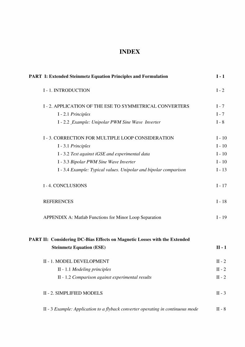
INDEX
PART I: Extended Steinmetz Equation Principles and Formulation I - 1
I - 1. INTRODUCTION I - 2
I - 2. APPLICATION OF THE ESE TO SYMMETRICAL CONVERTERS I - 7
I - 2.1 Principles I - 7
I - 2.2 Example: Unipolar PWM Sine Wave Inverter I - 8
I - 3. CORRECTION FOR MULTIPLE LOOP CONSIDERATION I - 10
I - 3.1 Principles I - 10
I - 3.2 Test against iGSE and experimental data I - 10
I - 3.3 Bipolar PWM Sine Wave Inverter I - 10
I - 3.4 Example: Typical values. Unipolar and bipolar comparison I - 13
I - 4. CONCLUSIONS I - 17
REFERENCES I - 18
APPENDIX A: Matlab Functions for Minor Loop Separation I - 19
PART II: Considering DC-Bias Effects on Magnetic Losses with the Extended
Steinmetz Equation (ESE) II - 1
II - 1. MODEL DEVELOPMENT II - 2
II - 1.1 Modeling principles II - 2
II - 1.2 Comparison against experimental results II - 2
II - 2. SIMPLIFIED MODELS II - 3
II - 3 Example: Application to a flyback converter operating in continuous mode II - 8
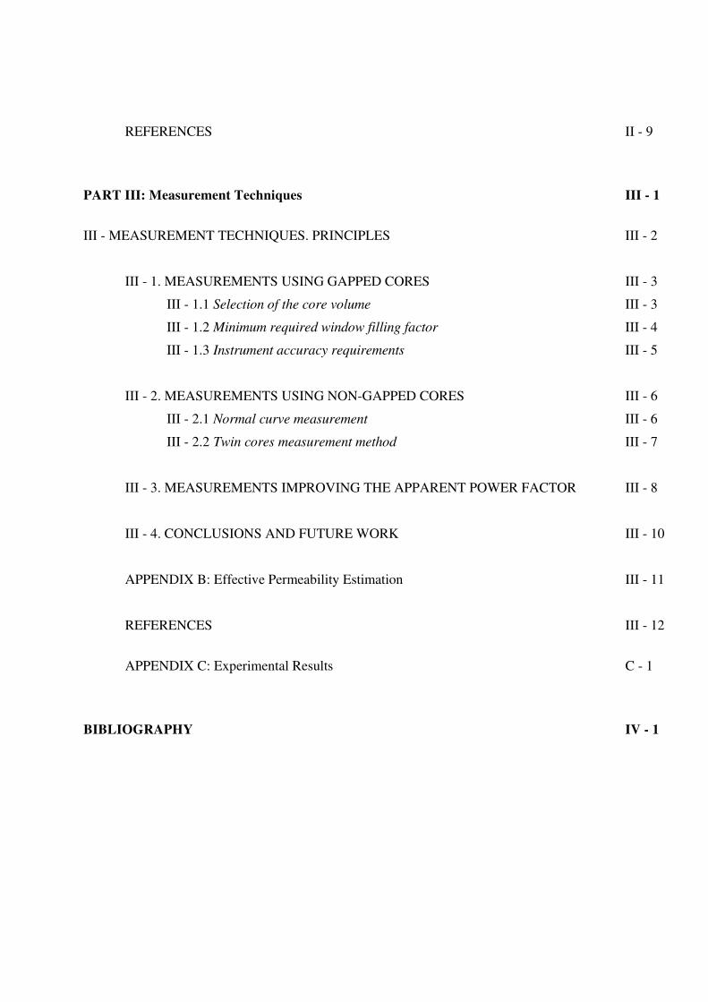
REFERENCES II - 9
PART III: Measurement Techniques III - 1
III - MEASUREMENT TECHNIQUES. PRINCIPLES III - 2
III - 1. MEASUREMENTS USING GAPPED CORES III - 3
III - 1.1 Selection of the core volume III - 3
III - 1.2 Minimum required window filling factor III - 4
III - 1.3 Instrument accuracy requirements III - 5
III - 2. MEASUREMENTS USING NON-GAPPED CORES III - 6
III - 2.1 Normal curve measurement III - 6
III - 2.2 Twin cores measurement method III - 7
III - 3. MEASUREMENTS IMPROVING THE APPARENT POWER FACTOR III - 8
III - 4. CONCLUSIONS AND FUTURE WORK III - 10
APPENDIX B: Effective Permeability Estimation III - 11
REFERENCES III - 12
APPENDIX C: Experimental Results C - 1
BIBLIOGRAPHY IV - 1
Extended Steinmetz Equation - I - 1
PART I
EXTENDED STEINMETZ EQUATION PRINCIPLES AND FORMULATION
Extended Steinmetz Equation - I - 2
I - 1. INTRODUCTION
Magnetic losses may be considered due to the hysteresis phenomenon and eddy current circulation inside
the core.
For sinusoidal waveforms, the hysteresis losses may be obtained from an empirical expression due to the
work of C. P. Steinmetz:
ςmh
Hv Bfk
Vol
Pp
H== (1.1.a)
where hk and ς are constant to be experimentally determined, while Bm is the maximum of the induction.
On the other hand, the eddy current losses are given by:
221
meE
v BfkVol
Pp
E ρ== (1.1.b)
where ρ is the core material resistivity.
In order to take account of the anomalous eddy current losses due to a non-homogeneous current
distribution (eddy currents), the resistivity may be assumed to be frequency dependent.
Thus, an approximative formula giving the total losses results:
( )221
mf
emhv BfkBfkVol
Pp
ρς +== (1.1.c)
To simplify the parameter extraction from experimental data, the above equation may be reduced to:
βαmsv Bfk
Vol
Pp == (1.2)
where sk , α , and β are constants to be determined from experimental data.
This last expression is usually known as Steinmetz equation.
Unfortunately, in power electronics most of the waveforms are not sinusoidal and eq. 1.2 is no longer
valid.
For non-sinusoidal waveforms the eddy current losses may be expressed as [1]:
( )
21
⎟⎟⎠
⎞⎜⎜⎝
⎛=
•rms
fEEv Bkpρ
(1.3.a)
while, for symmetrical waveforms without minor loops, the hysteresis losses remain expressed as function of the
induction amplitude mBB 2=Δ , as:
ς
⎟⎠⎞
⎜⎝⎛ Δ=
2
Bfkp HvH
(1.3.b).
Therefore, the total losses can be expressed as:
( )
21
2 ⎟⎟⎠
⎞⎜⎜⎝
⎛+⎟
⎠⎞
⎜⎝⎛ Δ=
•rms
fEHv Bk
Bfkp
ρ
ς (1.3.c).
A simplification similar to what was done with eq. 1.c may be introduced in order to transform the eq.
1.3.c into a single product: ζχ
ν⎟⎟⎠
⎞⎜⎜⎝
⎛⎟⎠⎞
⎜⎝⎛ Δ=
•rmsGv B
Bfkp
2 (1.4)
This equation is consistent with the classical Steinmetz expression, provided that appropriate values are
Extended Steinmetz Equation - I - 3
assigned to the constants Gk , ν , χ ,and ζ to force eq. 1.4 becoming equal to eq. 1.2 for sinusoidal
waveforms .
However, expression 1.4 has still an important drawback for cases other than pure sinusoids: A single
frequency has to be adopted to do calculations.
To overcome this limitation, an equivalent frequency is defined as:
B
B
dtdt
dB
TBf av
T
eq Δ=⎟⎟
⎠
⎞⎜⎜⎝
⎛Δ
=
•
∫ 2
11
2
1
0 (1.5)
(for pure sinewaves eq. 1.5 yields ffeq = ).
Substituting 1.5 into 1.4 yields:
ξεγ
⎟⎠⎞
⎜⎝⎛ Δ
⎟⎟⎠
⎞⎜⎜⎝
⎛⎟⎟⎠
⎞⎜⎜⎝
⎛==
••
2
BBBk
Vol
Pp
av
rmsmv (1.6.a)
where,
dtdt
dB
TB
T
rms
2
0
1∫ ⎟
⎠⎞
⎜⎝⎛=
• (1.6.b)
dtdt
dB
TB
T
av∫=
•
0
1 (1.6.c)
minmax BBB −=Δ (1.6.d)
for symmetrical waveforms it is mBB 2=Δ , where Bm is the amplitude of B(t) .
Equation 1.6.a is a Steinmetz-like expression generalized for non-sinusoidal operation, dependent on
dB/dt, but expressing it by means of analytical functions of B.
For sinusoidal waveforms eq. 1.6.a must match the classical Steinmetz equation 1.2.
Therefore:
( ) εγπ 42ms kk = (1.7.a)
εγα += (1.7.b)
εξγβ ++= (1.7.c)
From eqs. 1.7 the following expression results:
( )
αβεεα
εα
ππ
−•−•⎟⎠⎞
⎜⎝⎛ Δ
⎟⎟⎠
⎞⎜⎜⎝
⎛⎟⎟⎠
⎞⎜⎜⎝
⎛
⎟⎟⎠
⎞⎜⎜⎝
⎛==
28
2
BBB
k
Vol
Pp
av
rmss
v (1.8).
Eq. 1.8 will be named the Extended Steinmetz Equation (ESE) . It includes a parameter ε , which
modifies the rise of the plotted function (loss vs. duty cycle). This parameter should be determined looking for the
best fit with experimental data.
Another modified Steinmetz equation, the iGSE [2][3] proved to match the measured experimental values
well, so the ESE will be compared against the iGSE when experimental values are not available.
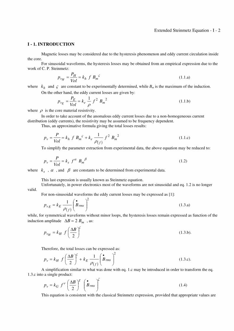
In Fig. 1.1 , the ESE is compared with results obtained from the iGSE , for a triangular waveform with
Extended Steinmetz Equation - I - 4
variable duty cycle D , using a ferrite core made of 3C85 material [2]. For this material, the best ε value is 0.9 ,
which gives the best agreement with the iGSE.
For others materials, the optimal ε varies.
It is found that the optimal ε does not depend on β nor ks , but it is affected by α .
As α usually ranges from 1.1 to 1.7 , a linear function is proposed for ε :
αε εε 21 kk += (1.9).
For 7.11.1 ≤≤α a good match with the iGSE (and also with experimental data) is obtained adopting:
αε 86.02 −= (1.10).
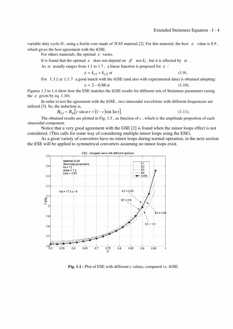
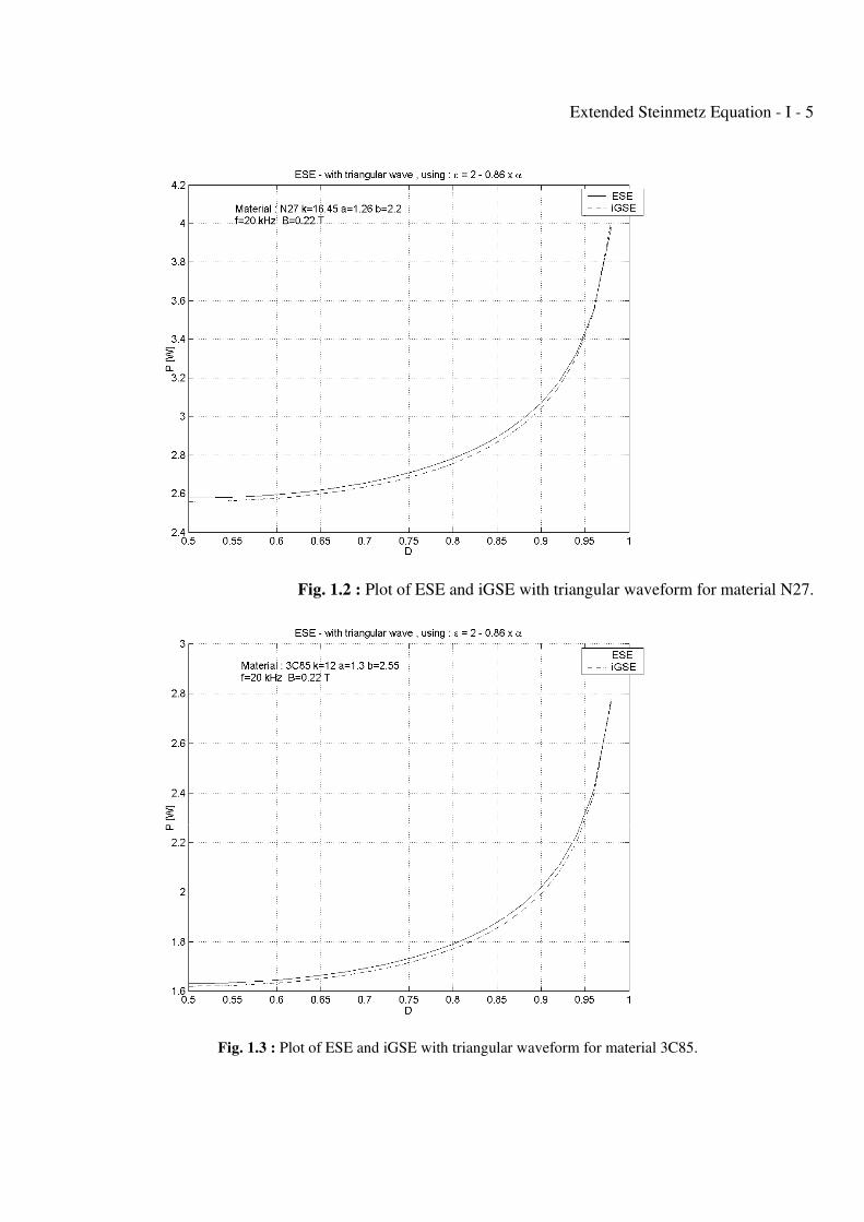
Figures 1.2 to 1.4 show how the ESE matches the iGSE results for different sets of Steinmetz parameters (using
the ε given by eq. 1.10).
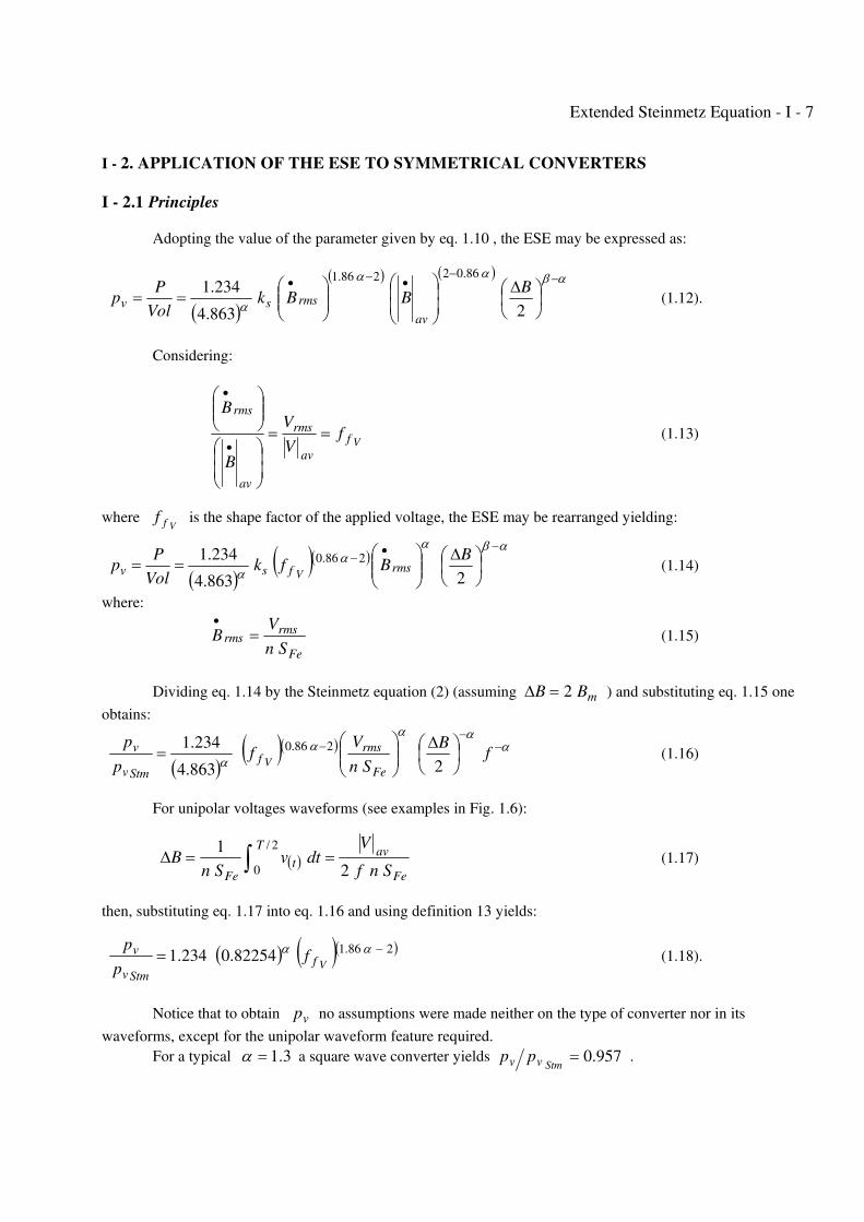
In order to test the agreement with the iGSE , two sinusoidal waveforms with different frequencies are
utilized [3]. So, the induction is,
( ) ( )[ ]tctcBB mt ωω 3sin1sin −+= (1.11).
The obtained results are plotted in Fig. 1.5 , as function of c , which is the amplitude proportion of each
sinusoidal component.
Notice that a very good agreement with the GSE [2] is found when the minor loops effect is not
considered. (This calls for some way of considering multiple minor loops using the ESE).
As a great variety of converters have no minor loops during normal operation, in the next section
the ESE will be applied to symmetrical converters assuming no minor loops exist.
Fig. 1.1 : Plot of ESE with different ε values, compared vs. iGSE.
Extended Steinmetz Equation - I - 5
Fig. 1.2 : Plot of ESE and iGSE with triangular waveform for material N27.
Fig. 1.3 : Plot of ESE and iGSE with triangular waveform for material 3C85.
Extended Steinmetz Equation - I - 6
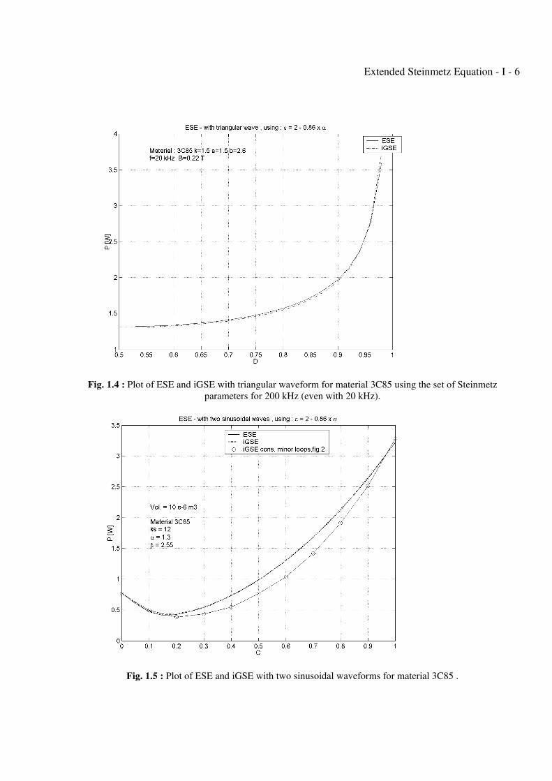
Fig. 1.4 : Plot of ESE and iGSE with triangular waveform for material 3C85 using the set of Steinmetz
parameters for 200 kHz (even with 20 kHz).
Fig. 1.5 : Plot of ESE and iGSE with two sinusoidal waveforms for material 3C85 .
Extended Steinmetz Equation - I - 7
I - 2. APPLICATION OF THE ESE TO SYMMETRICAL CONVERTERS I - 2.1 Principles
Adopting the value of the parameter given by eq. 1.10 , the ESE may be expressed as:
( )
( ) ( ) αβαα
α
−−•−•
⎟⎠⎞
⎜⎝⎛ Δ
⎟⎟⎠
⎞⎜⎜⎝
⎛⎟⎟⎠
⎞⎜⎜⎝
⎛==
2863.4
234.186.02286.1
BBBk
Vol
Pp
av
rmssv (1.12).
Considering:
Vf
av
rms
av
rms
fV
V
B
B
==
⎟⎟⎠
⎞⎜⎜⎝
⎛
⎟⎟⎠
⎞⎜⎜⎝
⎛
•
•
(1.13)
where Vff is the shape factor of the applied voltage, the ESE may be rearranged yielding:
( )( )( )
αβαα
α
−•− ⎟
⎠⎞
⎜⎝⎛ Δ
⎟⎟⎠
⎞⎜⎜⎝
⎛==
2863.4
234.1 286.0 BBfk
Vol
Pp rmsfsv V
(1.14)
where:
Fe
rmsrms
Sn
VB =•
(1.15)
Dividing eq. 1.14 by the Steinmetz equation (2) (assuming mBB 2=Δ ) and substituting eq. 1.15 one
obtains:
( )( )( ) α
ααα
α−
−− ⎟
⎠⎞
⎜⎝⎛ Δ
⎟⎟⎠
⎞⎜⎜⎝
⎛= f
B
Sn
Vf
p
p
Fe
rmsf
Stmv
v
V 2863.4
234.1 286.0 (1.16)
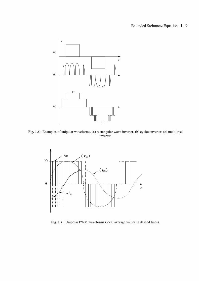
For unipolar voltages waveforms (see examples in Fig. 1.6):
( )Fe
avT
tFe Snf
Vdtv
SnB
2
1 2/
0==Δ ∫ (1.17)
then, substituting eq. 1.17 into eq. 1.16 and using definition 13 yields:
( ) ( )( )286.182254.0234.1
−= ααVf
Stmv
v fp
p (1.18).
Notice that to obtain vp no assumptions were made neither on the type of converter nor in its
waveforms, except for the unipolar waveform feature required.
For a typical 3.1=α a square wave converter yields 957.0=Stmvv pp .
Extended Steinmetz Equation - I - 8
A rectangular wave inverter having a sinusoidal equivalent wave shape factor of 11.1=Vf
f (duty =
0.812) gives 19996.0 ≅=Stmvv pp . For a duty-cycle of 0.25 one obtains 28.1=
Stmvv pp , but this is a
quite small duty for typical nominal power operation.
Next, an example of application to a complex output waveform converter is presented.
I - 2.2 Example:
Unipolar PWM Sine Wave Inverter
For an inverter using unipolar PWM sine wave synthesis (as shown in Fig. 1.7), the average transformer
voltage must be:
( ) tVdV mtP ωsin= (E1.1)
where d(t) is the duty cycle required to produce the sinusoidal average value of the output signal. So,
( ) tV
Vd
P
mt ωsin= (E1.2).
If Pm VV = the rms voltage applied to the transformer becomes:
( ) P
T
P
T
tPrms VdttT
VdtdVT
Vπ
ω 2sin
22 2/
0
2/
0
2 === ∫∫ (E1.3)
and the average rectified value results:
( ) P
T
tPavVdtdV
TV
π22 2/
0== ∫ (E1.4).
Therefore, the voltage shape factor is: 2533.12==
πVf
f . From eq. 18, for 3.1=α this yields:
10.1=Stmvv pp (E1.5)
A 10% of increase over the magnetic losses obtained from the classical Steinmetz equation should be
expected in a transformer used for this application.
Extended Steinmetz Equation - I - 9
Fig. 1.6 : Examples of unipolar waveforms, (a) rectangular wave inverter, (b) cycloconverter, (c) multilevel
inverter.
Fig. 1.7 : Unipolar PWM waveforms (local average values in dashed lines).
t
v
(a)
(b)
(c)
⟨ i(t) ⟩
⟨ v(t) ⟩ v(t)
i(t)
0
VP
t
Extended Steinmetz Equation - I - 10
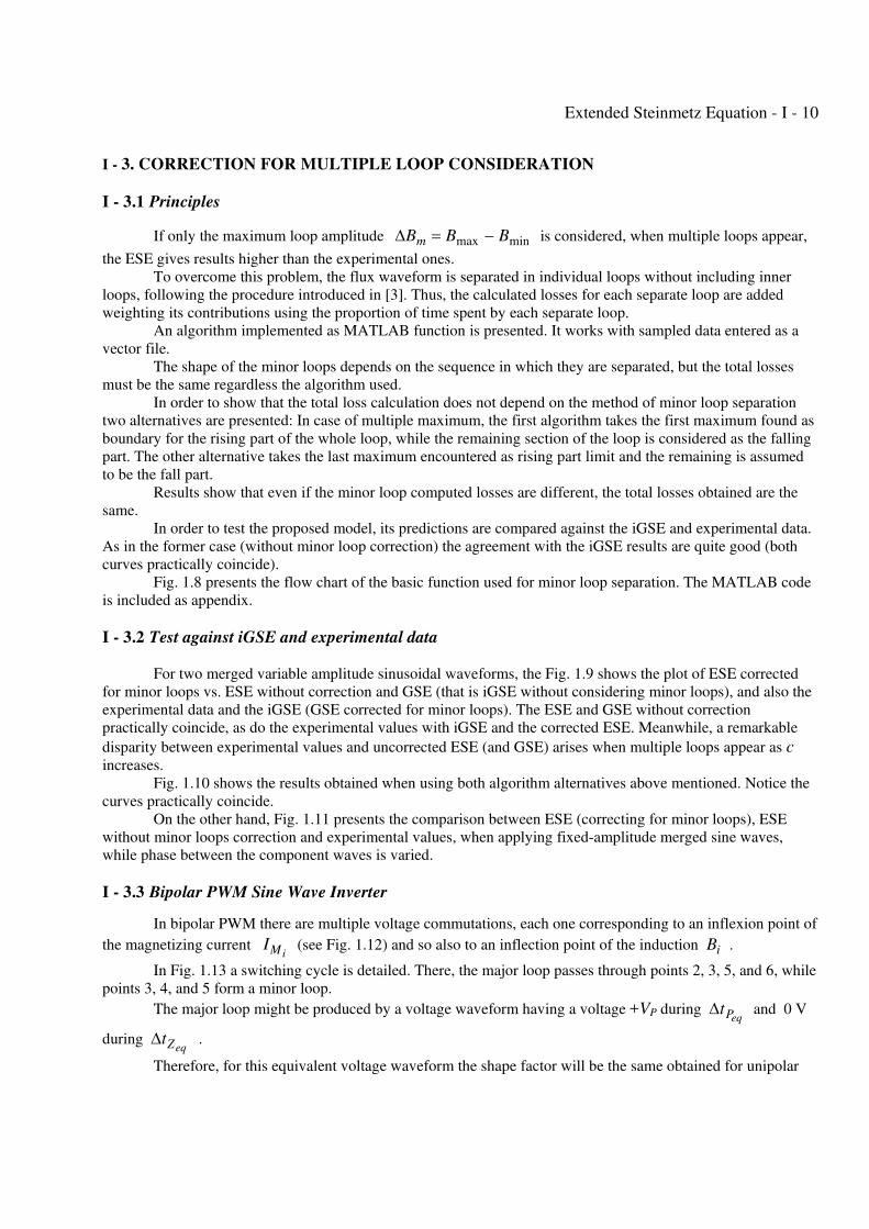
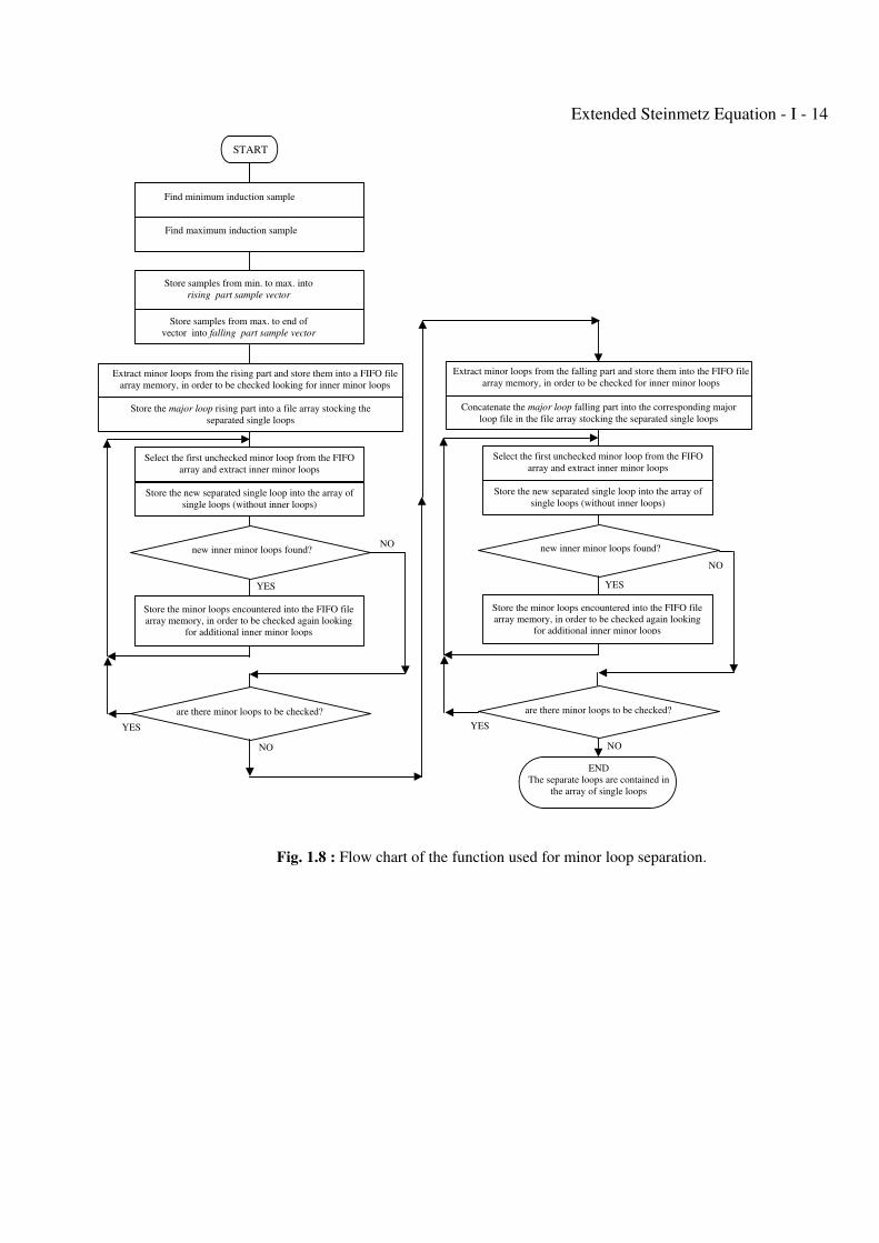
I - 3. CORRECTION FOR MULTIPLE LOOP CONSIDERATION
I - 3.1 Principles
If only the maximum loop amplitude minmax BBBm −=Δ is considered, when multiple loops appear,
the ESE gives results higher than the experimental ones.
To overcome this problem, the flux waveform is separated in individual loops without including inner
loops, following the procedure introduced in [3]. Thus, the calculated losses for each separate loop are added
weighting its contributions using the proportion of time spent by each separate loop.
An algorithm implemented as MATLAB function is presented. It works with sampled data entered as a
vector file.
The shape of the minor loops depends on the sequence in which they are separated, but the total losses
must be the same regardless the algorithm used.
In order to show that the total loss calculation does not depend on the method of minor loop separation
two alternatives are presented: In case of multiple maximum, the first algorithm takes the first maximum found as
boundary for the rising part of the whole loop, while the remaining section of the loop is considered as the falling
part. The other alternative takes the last maximum encountered as rising part limit and the remaining is assumed
to be the fall part.
Results show that even if the minor loop computed losses are different, the total losses obtained are the
same.
In order to test the proposed model, its predictions are compared against the iGSE and experimental data.
As in the former case (without minor loop correction) the agreement with the iGSE results are quite good (both
curves practically coincide).
Fig. 1.8 presents the flow chart of the basic function used for minor loop separation. The MATLAB code
is included as appendix.
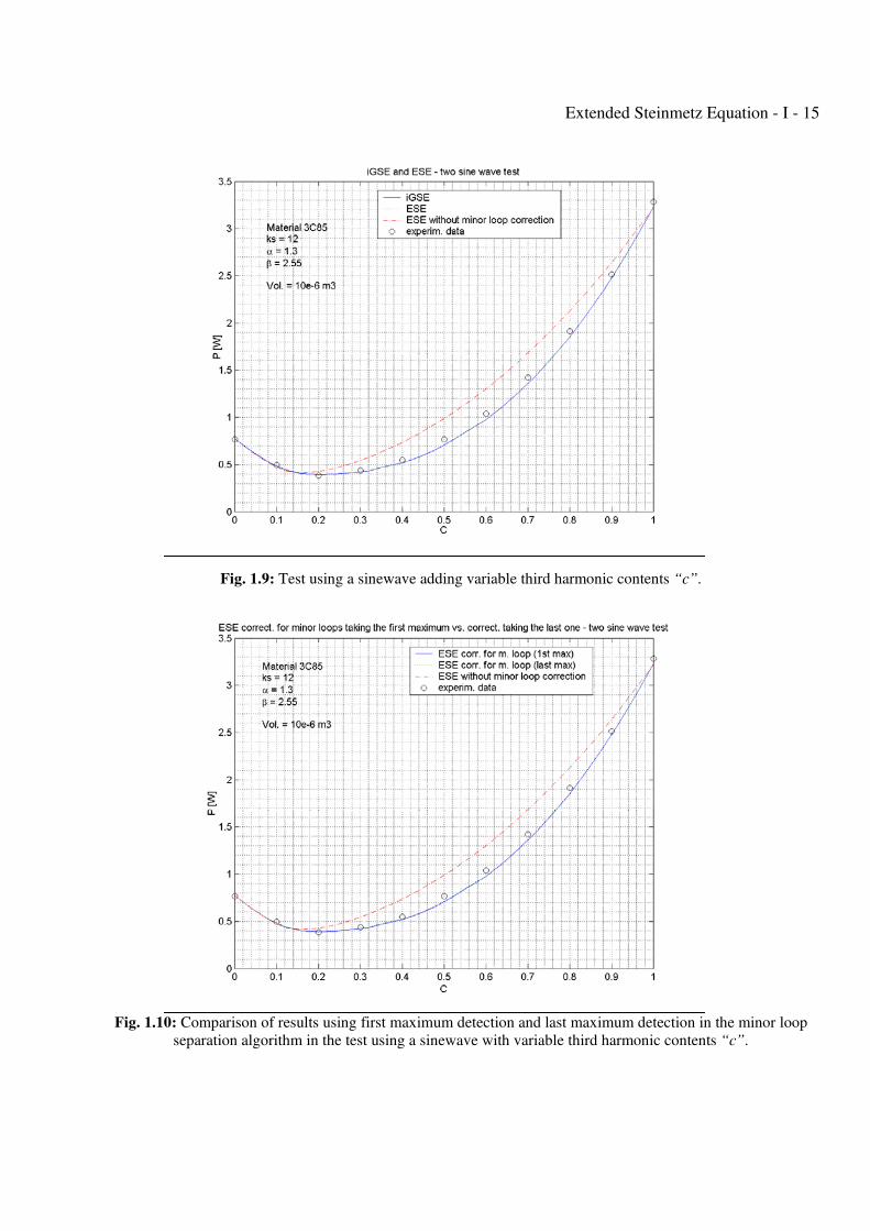
I - 3.2 Test against iGSE and experimental data
For two merged variable amplitude sinusoidal waveforms, the Fig. 1.9 shows the plot of ESE corrected
for minor loops vs. ESE without correction and GSE (that is iGSE without considering minor loops), and also the
experimental data and the iGSE (GSE corrected for minor loops). The ESE and GSE without correction
practically coincide, as do the experimental values with iGSE and the corrected ESE. Meanwhile, a remarkable
disparity between experimental values and uncorrected ESE (and GSE) arises when multiple loops appear as c
increases.
Fig. 1.10 shows the results obtained when using both algorithm alternatives above mentioned. Notice the
curves practically coincide.
On the other hand, Fig. 1.11 presents the comparison between ESE (correcting for minor loops), ESE
without minor loops correction and experimental values, when applying fixed-amplitude merged sine waves,
while phase between the component waves is varied.
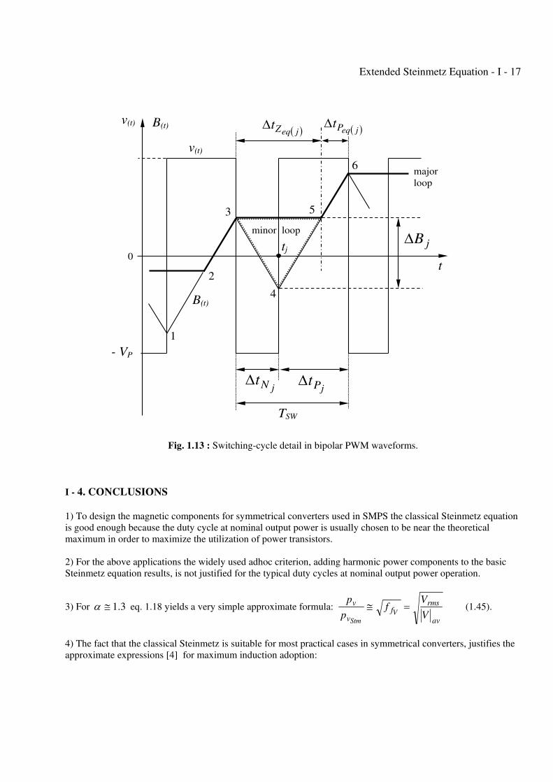
I - 3.3 Bipolar PWM Sine Wave Inverter
In bipolar PWM there are multiple voltage commutations, each one corresponding to an inflexion point of
the magnetizing current iMI (see Fig. 1.12) and so also to an inflection point of the induction iB .
In Fig. 1.13 a switching cycle is detailed. There, the major loop passes through points 2, 3, 5, and 6, while
points 3, 4, and 5 form a minor loop.
The major loop might be produced by a voltage waveform having a voltage +VP duringeqPtΔ and 0 V
duringeqZtΔ .
Therefore, for this equivalent voltage waveform the shape factor will be the same obtained for unipolar
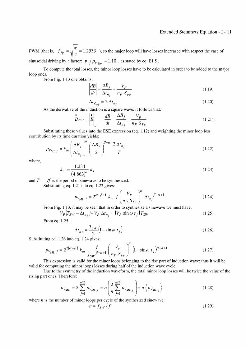
Extended Steinmetz Equation - I - 11
PWM (that is, 2533.12==
πVf
f ), so the major loop will have losses increased with respect the case of
sinusoidal driving by a factor: 10.1=Stmvv pp , as stated by eq. E1.5 .
To compute the total losses, the minor loop losses have to be calculated in order to be added to the major
loop ones.
From Fig. 1.13 one obtains:
FeP
P
n
j
Sn
V
t
B
dt
dB
j
=Δ
Δ= (1.19)
jeq nZ tt Δ=Δ 2 (1.20).
As the derivative of the induction is a square wave, it follows that:
FeP
P
n
j
av
rmsSn
V
t
B
dt
dBBB
j
=Δ
Δ===
•• (1.21).
Substituting these values into the ESE expression (eq. 1.12) and weighting the minor loop loss
contribution by its time duration yields:
T
tB
t
Bkp
j
j
jML
nj
n
jmV
Δ⎟⎟⎠
⎞⎜⎜⎝
⎛ Δ⎟⎟
⎠
⎞
⎜⎜
⎝
⎛
Δ
Δ=
− 2
2
αβα
(1.22)
where,
( ) sm kk α
863.4
234.1= (1.23)
and T = 1/f is the period of sinewave to be synthesized.
Substituting eq. 1.21 into eq. 1.22 gives:
112+−+− Δ⎟⎟
⎠
⎞⎜⎜⎝
⎛= αβ
ββα
jML nFeP
PmjV t
Sn
Vfkp (1.24).
From Fig. 1.13, it may be seen that in order to synthesize a sinewave we must have:
( ) ( ) SWjPnPnSWP TtVtVtTVjj
ωsin=Δ−Δ− (1.25).
From eq. 1.25 :
( )jSW
n tT
tj
ωsin12
−=Δ (1.26).
Substituting eq. 1.26 into eq. 1.24 gives:
( ) ( ) 1
1
2 sin12+−
+−− −⎟⎟
⎠
⎞⎜⎜⎝
⎛= αβ
β
αββα ω j
FeP
P
SW
mjV tSn
V
f
fkp
ML (1.27).
This expression is valid for the minor loops belonging to the rise part of induction wave; thus it will be
valid for computing the minor loops losses during half of the induction wave cycle.
Due to the symmetry of the induction waveform, the total minor loop losses will be twice the value of the
rising part ones. Therefore:
jMLjMLjMLML V
n
j
V
n
j
VV pnpn
npp =⎟⎟
⎠
⎞
⎜⎜
⎝
⎛== ∑∑
==
2
1
2
1
22 (1.28)
where n is the number of minor loops per cycle of the synthesized sinewave:
ffn SW= (1.29).
Extended Steinmetz Equation - I - 12
As ffSW >> the discrete average may be approximated by the integral average and using eq. 1.29 it
results:
( ) ( ) ⎟
⎠⎞
⎜⎝⎛ −⎟⎟
⎠
⎞⎜⎜⎝
⎛= ∫ +−−− θθ
ππ αβ
ββαβα d
Sn
Vfkp
FeP
PSWmVML
2
0
12 sin12
2 (1.30).
The integral between brackets should be calculated numerically but for 315.1 ≤+−≤ αβ it may be
approximated with less than 0.6 % of error by:
( )( ) 75.0
2
0
1
1
38.0sin1
2
+−≅⎟
⎠⎞
⎜⎝⎛ −= ∫ +−
αβθθ
ππ αβ
dS (1.31).
Usually 21 ≅+−αβ and the integral approaches the value 0.23.
Substituting eqs. 1.23 and 1.31 into eq. 1.30 yields:
( ) ( ) SSn
Vfkp
FeP
PSWsVML
ββααβ
⎟⎟⎠
⎞⎜⎜⎝
⎛= −
8225.025.0234.1 (1.32).
Dividing eq. 1.32 by the Steinmetz’s equation:
( ) ( )
SBSn
V
ffp
p
mFeP
P
SWV
V
Stm
ML
β
αβ
αβ
⎟⎟⎠
⎞⎜⎜⎝
⎛=
−8225.025.0
234.1 (1.33)
where,
2
2/SW
m
T
Sm
BBB
Δ+= (1.34)
is the maximum induction value, mSB is the peak value of the sinusoidal local average induction, and
2/SWTBΔ is the amplitude of the alternative high frequency component of the induction, when it reaches it
maximum value. This happens each time the primary local average voltage crosses through zero. Therefore, the
duty cycle must be 1/2, which yields:
FePSW
PT
Snf
VB
SW 22/ =Δ (1.35).
Assuming a primary peak voltage for the synthesized sinewave equal to VP , from Faraday’s law one
obtains:
mSFePP BSnfV π2= (1.36).
Substituting eqs. 1.34, 1.35 and 1.36 into eq. 1.33 yields:
( ) ( )
S
f
f
f
ffp
p
SW
SW
SWV
V
Stm
ML
β
αβ
αβ
π ⎟⎟⎟⎟
⎠
⎞
⎜⎜⎜⎜
⎝
⎛
+=
− 21
48225.025.0234.1 (1.37).
Assuming ffSW
>> the eq. 1.37 becomes:
( ) ( ) ( ) Sf
ffp
p
SWV
V
Stm
ML βαβ
αβπ2
8225.025.0234.1
−=
which may be rearranged as:
( )( )
Sff
f
p
p
SWV
V
Stm
ML
αβ
αβα π
−
−
⎟⎠⎞
⎜⎝⎛=
1
28225.0234.1 (1.38).
Extended Steinmetz Equation - I - 13
Also, using eqs. 1.21, 1.35 and 1.36 one obtains the maximum value of the minor loop amplitude
normalized to the sinusoidal induction amplitude:
] ( )
SWS
SW
S
T
S
ML
f
f
B
TdtdB
B
B
B
B
mm
SW
m
π==Δ
=Δ 22/max
(1.39).
I - 3.4 Example: Typical values. Unipolar and bipolar comparison
For typical values 3.1=α , 5.2=β , 100=ffSW and Hzf 60= , eqs. 1.38 and 1.39 give:
0085.0=Stm
ML
V
V
p
p and 0031.0
max =Δ
mS
ML
B
B.
For the same values but 20=ffSW one obtains 0586.0=Stm
ML
V
V
p
p.
Therefore, for the most practical cases in bipolar PWM, the increase of losses due to minor loops may be
neglected, and only the expression obtained for unipolar PWM (eq. E1.5) may be used for design purposes.
Notice that the actual voltage shape factor in bipolar PWM is 1=Vf
f . Thus, a direct utilization of the
actual voltage waveform in the eq. 1.18 (instead of the shape factor of the equivalent voltage waveform) will give
wrong results, lower than the ones obtained from the classical Steinmetz equation. This is because,
( ) ( )∫∫ ==2
0
2
0
22 T
t
T
tavdtv
Tdtv
TV (which is only valid for unipolar waveforms), in the eq. 1.18 derivation.
On the other hand, substituting the actual induction vector in the ESE, without taking account of minor
loops, yields values higher than the real ones. In such a case:
max
max2
2MLSW
SW
ML
av
rms BfT
B
dt
dBBB Δ=
Δ===
•• (1.40)
max2 MLS BBB
mΔ+=Δ (1.41).
Substituting these values into the ESE expression (eq. 1.12) and dividing by the classical Steinmetz
expression:
( )( )
α
αα
α ⎟⎟⎠
⎞⎜⎜⎝
⎛
⎟⎟⎟
⎠
⎞
⎜⎜⎜
⎝
⎛
Δ+
=f
f
B
Bp
pSW
ML
SV
V
mStm
ML
max2
1
12
863.4
234.1 (1.42).
If ffSW
>> then maxMLS BB
mΔ>> , and the eq. 1.42 becomes:
( )( )
αα
αα ⎟⎟
⎠
⎞⎜⎜⎝
⎛⎟⎟⎟
⎠
⎞
⎜⎜⎜
⎝
⎛ Δ≅
f
f
B
B
p
pSW
S
ML
V
V
mStm
ML max2
863.4
234.1 (1.43).
Substituting eq. 1.39 into eq. 1.43 yields:
( )( ) ( )αα
α π 292.1234.12863.4
234.1=≅
Stm
ML
V
V
p
p (1.44).
For a typical value of 3.1=α , eq. 1.44 gives: 722.1=Stm
ML
V
V
p
p, which is a value too high.
Extended Steinmetz Equation - I - 14
Fig. 1.8 : Flow chart of the function used for minor loop separation.
START
Find minimum induction sample
Find maximum induction sample
Store samples from min. to max. into
rising part sample vector
Store samples from max. to end of
vector into falling part sample vector
Extract minor loops from the rising part and store them into a FIFO file
array memory, in order to be checked looking for inner minor loops
Select the first unchecked minor loop from the FIFO
array and extract inner minor loops
new inner minor loops found?
YES
Store the minor loops encountered into the FIFO file
array memory, in order to be checked again looking
for additional inner minor loops
Store the major loop rising part into a file array stocking the
separated single loops
Store the new separated single loop into the array of
single loops (without inner loops)
NO
are there minor loops to be checked?
NO
YES
Extract minor loops from the falling part and store them into the FIFO file
array memory, in order to be checked for inner minor loops
Select the first unchecked minor loop from the FIFO
array and extract inner minor loops
new inner minor loops found?
YES
Store the minor loops encountered into the FIFO file
array memory, in order to be checked again looking
for additional inner minor loops
Concatenate the major loop falling part into the corresponding major
loop file in the file array stocking the separated single loops
Store the new separated single loop into the array of
single loops (without inner loops)
NO
are there minor loops to be checked?
NO
YES
END
The separate loops are contained in
the array of single loops
Extended Steinmetz Equation - I - 15
Fig. 1.9: Test using a sinewave adding variable third harmonic contents “c”.
Fig. 1.10: Comparison of results using first maximum detection and last maximum detection in the minor loop
separation algorithm in the test using a sinewave with variable third harmonic contents “c”.
Extended Steinmetz Equation - I - 16
Fig. 1.11: Test using two added sinewaves with c = 0.7 and variable phase.
Fig. 1.12 : Bipolar PWM waveforms (local average values in dashed lines).
⟨ i(t) ⟩ ⟨ v(t) ⟩ v(t)
i(t)
0
- VP
t
VP
Extended Steinmetz Equation - I - 17
Fig. 1.13 : Switching-cycle detail in bipolar PWM waveforms.
I - 4. CONCLUSIONS 1) To design the magnetic components for symmetrical converters used in SMPS the classical Steinmetz equation
is good enough because the duty cycle at nominal output power is usually chosen to be near the theoretical
maximum in order to maximize the utilization of power transistors.
2) For the above applications the widely used adhoc criterion, adding harmonic power components to the basic
Steinmetz equation results, is not justified for the typical duty cycles at nominal output power operation.
3) For 3.1≅α eq. 1.18 yields a very simple approximate formula:
av
rmsf
v
v
V
Vf
p
pV
Stm
=≅ (1.45).
4) The fact that the classical Steinmetz is suitable for most practical cases in symmetrical converters, justifies the
approximate expressions [4] for maximum induction adoption:
jBΔ
t
( )jeqZtΔ
jPtΔjNtΔ
TSW
1
2
3
4
5
6
( )jeqPtΔ
- VP
tj
v(t) B(t)
B(t)
v(t)
major
loop
minor loop
0
Extended Steinmetz Equation - I - 18
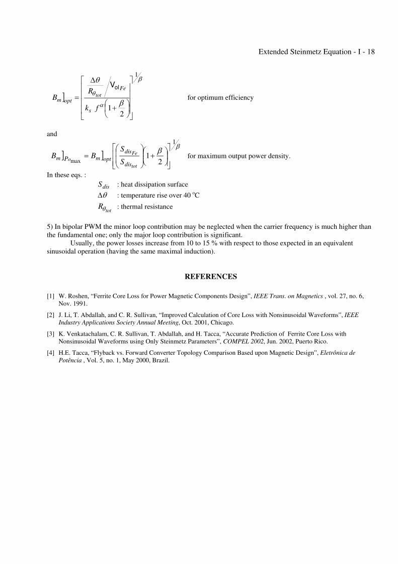
]
β
β
θ
α
θ
1
21 ⎥
⎥⎥⎥
⎦
⎤
⎢⎢⎢⎢
⎣
⎡
⎟⎠⎞
⎜⎝⎛ +
Δ
=fk
RB
s
Fe
optmtot
olV
for optimum efficiency
and
] ]ββ
1
21
max ⎥⎥⎦
⎤
⎢⎢⎣
⎡⎟⎠⎞
⎜⎝⎛ +⎟⎟⎠
⎞⎜⎜⎝
⎛=
tot
Fe
odis
dis
optmmS
SBB P for maximum output power density.
In these eqs. :
disS : heat dissipation surface
θΔ : temperature rise over 40 oC
totRθ : thermal resistance
5) In bipolar PWM the minor loop contribution may be neglected when the carrier frequency is much higher than
the fundamental one; only the major loop contribution is significant.
Usually, the power losses increase from 10 to 15 % with respect to those expected in an equivalent
sinusoidal operation (having the same maximal induction).
REFERENCES
[1] W. Roshen, “Ferrite Core Loss for Power Magnetic Components Design”, IEEE Trans. on Magnetics , vol. 27, no. 6,
Nov. 1991.
[2] J. Li, T. Abdallah, and C. R. Sullivan, “Improved Calculation of Core Loss with Nonsinusoidal Waveforms”, IEEE
Industry Applications Society Annual Meeting, Oct. 2001, Chicago.
[3] K. Venkatachalam, C. R. Sullivan, T. Abdallah, and H. Tacca, “Accurate Prediction of Ferrite Core Loss with
Nonsinusoidal Waveforms using Only Steinmetz Parameters”, COMPEL 2002, Jun. 2002, Puerto Rico.
[4] H.E. Tacca, “Flyback vs. Forward Converter Topology Comparison Based upon Magnetic Design”, Eletrônica de
Potência , Vol. 5, no. 1, May 2000, Brazil.
Extended Steinmetz Equation - I - 19
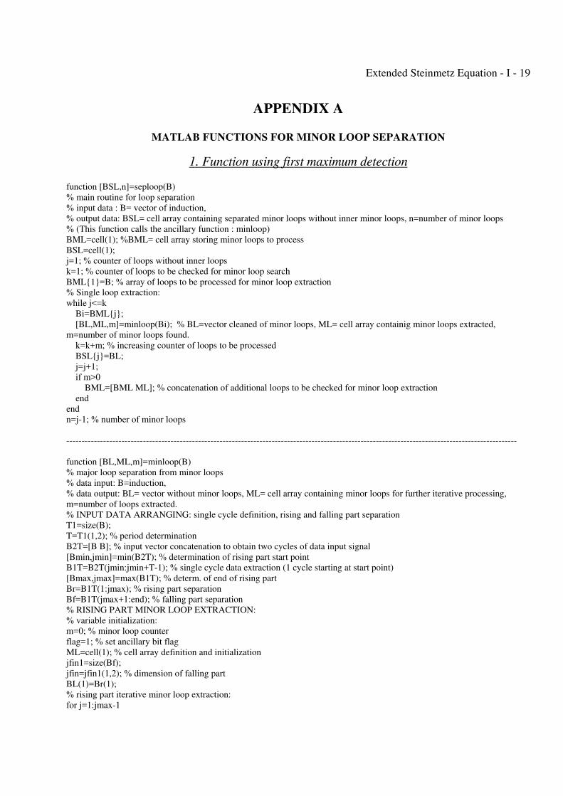
APPENDIX A
MATLAB FUNCTIONS FOR MINOR LOOP SEPARATION
1. Function using first maximum detection function [BSL,n]=seploop(B)
% main routine for loop separation
% input data : B= vector of induction,
% output data: BSL= cell array containing separated minor loops without inner minor loops, n=number of minor loops
% (This function calls the ancillary function : minloop)
BML=cell(1); %BML= cell array storing minor loops to process
BSL=cell(1);
j=1; % counter of loops without inner loops
k=1; % counter of loops to be checked for minor loop search
BML{1}=B; % array of loops to be processed for minor loop extraction
% Single loop extraction:
while j<=k
Bi=BML{j};
[BL,ML,m]=minloop(Bi); % BL=vector cleaned of minor loops, ML= cell array containig minor loops extracted,
m=number of minor loops found.
k=k+m; % increasing counter of loops to be processed
BSL{j}=BL;
j=j+1;
if m>0
BML=[BML ML]; % concatenation of additional loops to be checked for minor loop extraction
end
end
n=j-1; % number of minor loops
---------------------------------------------------------------------------------------------------------------------------------------------------
function [BL,ML,m]=minloop(B)
% major loop separation from minor loops
% data input: B=induction,
% data output: BL= vector without minor loops, ML= cell array containing minor loops for further iterative processing,
m=number of loops extracted.
% INPUT DATA ARRANGING: single cycle definition, rising and falling part separation
T1=size(B);
T=T1(1,2); % period determination
B2T=[B B]; % input vector concatenation to obtain two cycles of data input signal
[Bmin,jmin]=min(B2T); % determination of rising part start point
B1T=B2T(jmin:jmin+T-1); % single cycle data extraction (1 cycle starting at start point)
[Bmax,jmax]=max(B1T); % determ. of end of rising part
Br=B1T(1:jmax); % rising part separation
Bf=B1T(jmax+1:end); % falling part separation
% RISING PART MINOR LOOP EXTRACTION:
% variable initialization:
m=0; % minor loop counter
flag=1; % set ancillary bit flag
ML=cell(1); % cell array definition and initialization
jfin1=size(Bf);
jfin=jfin1(1,2); % dimension of falling part
BL(1)=Br(1);
% rising part iterative minor loop extraction:
for j=1:jmax-1
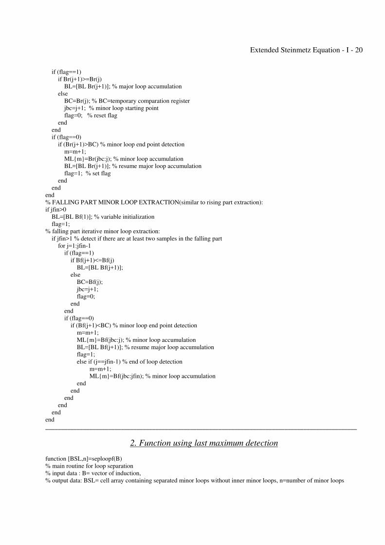
Extended Steinmetz Equation - I - 20
if (flag==1)
if Br(j+1)>=Br(j)
BL=[BL Br(j+1)]; % major loop accumulation
else
BC=Br(j); % BC=temporary comparation register
jbc=j+1; % minor loop starting point
flag=0; % reset flag
end
end
if (flag==0)
if (Br(j+1)>BC) % minor loop end point detection
m=m+1;
ML{m}=Br(jbc:j); % minor loop accumulation
BL=[BL Br(j+1)]; % resume major loop accumulation
flag=1; % set flag
end
end
end
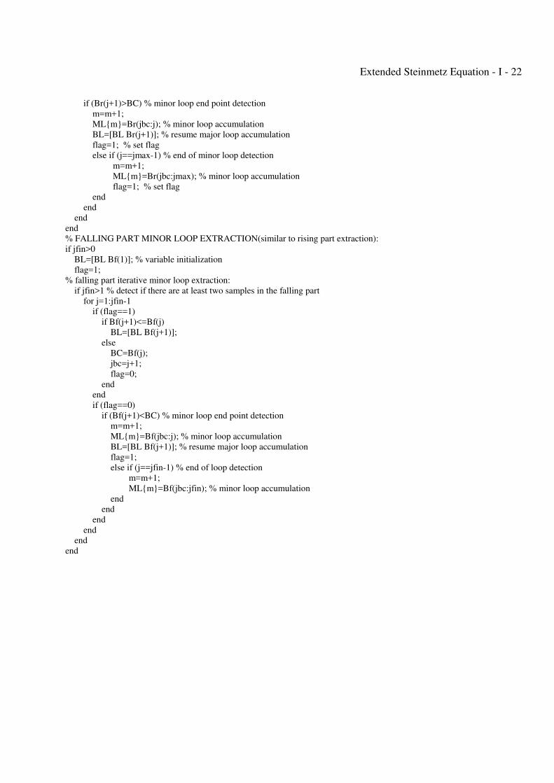
% FALLING PART MINOR LOOP EXTRACTION(similar to rising part extraction):
if jfin>0
BL=[BL Bf(1)]; % variable initialization
flag=1;
% falling part iterative minor loop extraction:
if jfin>1 % detect if there are at least two samples in the falling part
for j=1:jfin-1
if (flag==1)
if Bf(j+1)<=Bf(j)
BL=[BL Bf(j+1)];
else
BC=Bf(j);
jbc=j+1;
flag=0;
end
end
if (flag==0)
if (Bf(j+1)<BC) % minor loop end point detection
m=m+1;
ML{m}=Bf(jbc:j); % minor loop accumulation
BL=[BL Bf(j+1)]; % resume major loop accumulation
flag=1;
else if (j==jfin-1) % end of loop detection
m=m+1;
ML{m}=Bf(jbc:jfin); % minor loop accumulation
end
end
end
end
end
end
___________________________________________________________________________________________________
2. Function using last maximum detection
function [BSL,n]=seploopf(B)
% main routine for loop separation
% input data : B= vector of induction,
% output data: BSL= cell array containing separated minor loops without inner minor loops, n=number of minor loops
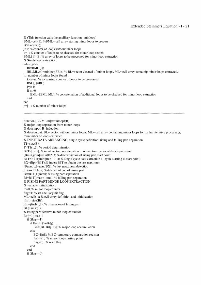
Extended Steinmetz Equation - I - 21
% (This function calls the ancillary function : minloop)
BML=cell(1); %BML= cell array storing minor loops to process
BSL=cell(1);
j=1; % counter of loops without inner loops
k=1; % counter of loops to be checked for minor loop search
BML{1}=B; % array of loops to be processed for minor loop extraction
% Single loop extraction:
while j<=k
Bi=BML{j};
[BL,ML,m]=minloopf(Bi); % BL=vector cleaned of minor loops, ML= cell array containig minor loops extracted,
m=number of minor loops found.
k=k+m; % increasing counter of loops to be processed
BSL{j}=BL;
j=j+1;
if m>0
BML=[BML ML]; % concatenation of additional loops to be checked for minor loop extraction
end
end
n=j-1; % number of minor loops
---------------------------------------------------------------------------------------------------------------------------------------------------
function [BL,ML,m]=minloopf(B)
% major loop separation from minor loops
% data input: B=induction,
% data output: BL= vector without minor loops, ML= cell array containing minor loops for further iterative processing,
m=number of loops extracted.
% INPUT DATA ARRANGING: single cycle definition, rising and falling part separation
T1=size(B);
T=T1(1,2); % period determination
B2T=[B B]; % input vector concatenation to obtain two cycles of data input signal
[Bmin,jmin]=min(B2T); % determination of rising part start point
B1T=B2T(jmin:jmin+T-1); % single cycle data extraction (1 cycle starting at start point)
BX=fliplr(B1T);% invert B1T to obtain the last maximum
[Bmax,jx]=max(BX); % last maximum detection
jmax= T+1-jx; % determ. of end of rising part
Br=B1T(1:jmax); % rising part separation
Bf=B1T(jmax+1:end); % falling part separation
% RISING PART MINOR LOOP EXTRACTION:
% variable initialization:
m=0; % minor loop counter
flag=1; % set ancillary bit flag
ML=cell(1); % cell array definition and initialization
jfin1=size(Bf);
jfin=jfin1(1,2); % dimension of falling part
BL(1)=Br(1);
% rising part iterative minor loop extraction:
for j=1:jmax-1
if (flag==1)
if Br(j+1)>=Br(j)
BL=[BL Br(j+1)]; % major loop accumulation
else
BC=Br(j); % BC=temporary comparation register
jbc=j+1; % minor loop starting point
flag=0; % reset flag
end
end
if (flag==0)
Extended Steinmetz Equation - I - 22
if (Br(j+1)>BC) % minor loop end point detection
m=m+1;
ML{m}=Br(jbc:j); % minor loop accumulation
BL=[BL Br(j+1)]; % resume major loop accumulation
flag=1; % set flag
else if (j==jmax-1) % end of minor loop detection
m=m+1;
ML{m}=Br(jbc:jmax); % minor loop accumulation
flag=1; % set flag
end
end
end
end
% FALLING PART MINOR LOOP EXTRACTION(similar to rising part extraction):
if jfin>0
BL=[BL Bf(1)]; % variable initialization
flag=1;
% falling part iterative minor loop extraction:
if jfin>1 % detect if there are at least two samples in the falling part
for j=1:jfin-1
if (flag==1)
if Bf(j+1)<=Bf(j)
BL=[BL Bf(j+1)];
else
BC=Bf(j);
jbc=j+1;
flag=0;
end
end
if (flag==0)
if (Bf(j+1)<BC) % minor loop end point detection
m=m+1;
ML{m}=Bf(jbc:j); % minor loop accumulation
BL=[BL Bf(j+1)]; % resume major loop accumulation
flag=1;
else if (j==jfin-1) % end of loop detection
m=m+1;
ML{m}=Bf(jbc:jfin); % minor loop accumulation
end
end
end
end
end
end
Extended Steinmetz Equation - II - 1
PART II
CONSIDERING DC-BIAS EFFECTS ON MAGNETIC LOSSES WITH THE EXTENDED STEINMETZ EQUATION (ESE)
Extended Steinmetz Equation - II - 2
II - CONSIDERING DC-BIAS EFFECTS ON MAGNETIC LOSSES WITH
THE EXTENDED STEINMETZ EQUATION (ESE)
II - 1. MODEL DEVELOPMENT
II - 1.1 Modeling principles
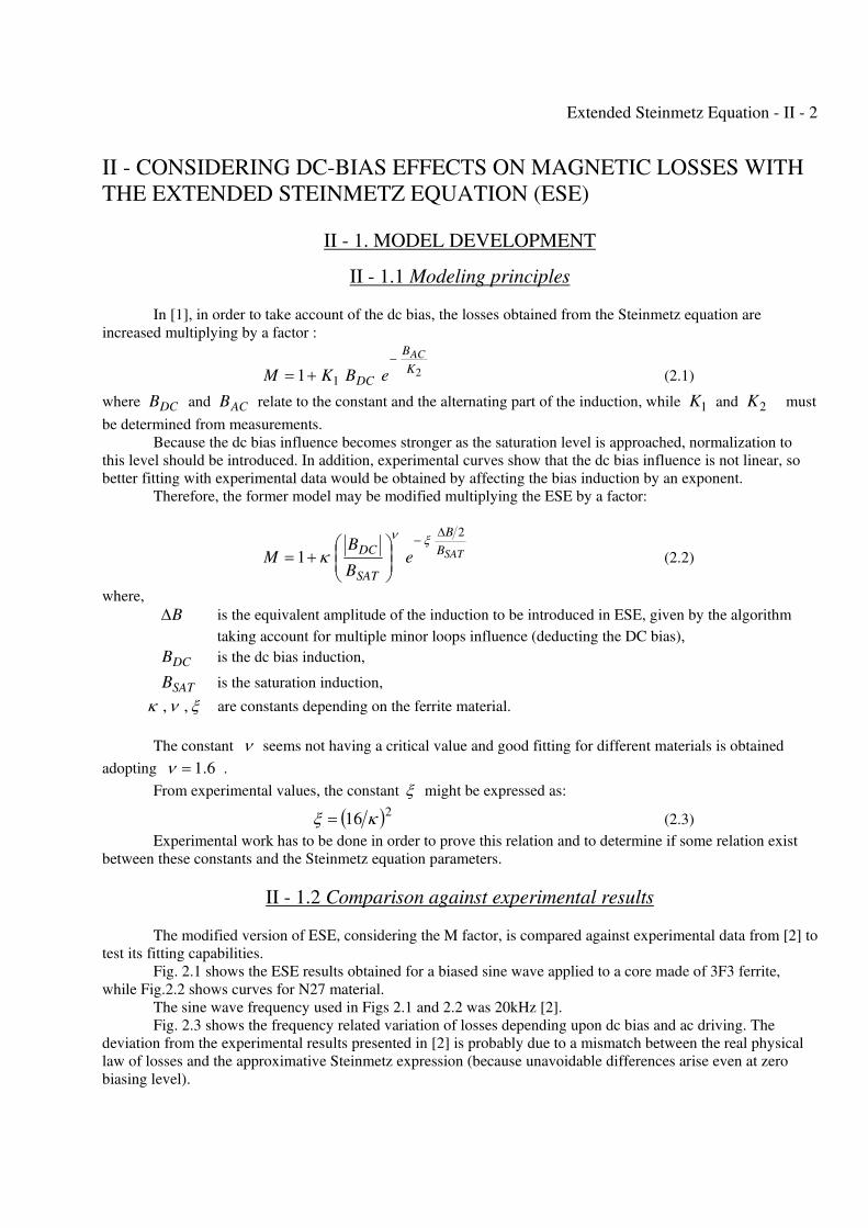
In [1], in order to take account of the dc bias, the losses obtained from the Steinmetz equation are
increased multiplying by a factor :
211
K
B
DC
AC
eBKM−
+= (2.1)
where DCB and ACB relate to the constant and the alternating part of the induction, while 1K and 2K must
be determined from measurements.
Because the dc bias influence becomes stronger as the saturation level is approached, normalization to
this level should be introduced. In addition, experimental curves show that the dc bias influence is not linear, so
better fitting with experimental data would be obtained by affecting the bias induction by an exponent.
Therefore, the former model may be modified multiplying the ESE by a factor:
SATB
B
SAT
DCe
B
BM
2
1
Δ−
⎟⎟⎠
⎞⎜⎜⎝
⎛+=
ξν
κ (2.2)
where,
BΔ is the equivalent amplitude of the induction to be introduced in ESE, given by the algorithm
taking account for multiple minor loops influence (deducting the DC bias),
DCB is the dc bias induction,
SATB is the saturation induction,
ξνκ ,, are constants depending on the ferrite material.
The constant ν seems not having a critical value and good fitting for different materials is obtained
adopting 6.1=ν .
From experimental values, the constant ξ might be expressed as:
( )216 κξ = (2.3)
Experimental work has to be done in order to prove this relation and to determine if some relation exist
between these constants and the Steinmetz equation parameters.
II - 1.2 Comparison against experimental results
The modified version of ESE, considering the M factor, is compared against experimental data from [2] to
test its fitting capabilities.
Fig. 2.1 shows the ESE results obtained for a biased sine wave applied to a core made of 3F3 ferrite,
while Fig.2.2 shows curves for N27 material.
The sine wave frequency used in Figs 2.1 and 2.2 was 20kHz [2].
Fig. 2.3 shows the frequency related variation of losses depending upon dc bias and ac driving. The
deviation from the experimental results presented in [2] is probably due to a mismatch between the real physical
law of losses and the approximative Steinmetz expression (because unavoidable differences arise even at zero
biasing level).
Extended Steinmetz Equation - II - 3
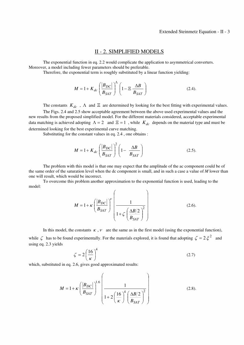
II - 2. SIMPLIFIED MODELS
The exponential function in eq. 2.2 would complicate the application to asymmetrical converters.
Moreover, a model including fewer parameters should be preferable.
Therefore, the exponential term is roughly substituted by a linear function yielding:
⎟⎟⎠
⎞⎜⎜⎝
⎛ ΔΞ−⎟⎟
⎠
⎞⎜⎜⎝
⎛+=
Λ
SATSAT
DCdc
B
B
B
BKM 11 (2.4).
The constants dcK , Λ and Ξ are determined by looking for the best fitting with experimental values.
The Figs. 2.4 and 2.5 show acceptable agreement between the above used experimental values and the
new results from the proposed simplified model. For the different materials considered, acceptable experimental
data matching is achieved adopting 2=Λ and 1=Ξ , while dcK depends on the material type and must be
determined looking for the best experimental curve matching.
Substituting for the constant values in eq. 2.4 , one obtains :
⎟⎟⎠
⎞⎜⎜⎝
⎛ Δ−⎟⎟
⎠
⎞⎜⎜⎝
⎛+=
SATSAT
DCdc
B
B
B
BKM 11
2
(2.5).
The problem with this model is that one may expect that the amplitude of the ac component could be of
the same order of the saturation level when the dc component is small, and in such a case a value of M lower than
one will result, which would be incorrect.
To overcome this problem another approximation to the exponential function is used, leading to the
model:
⎟⎟⎟⎟⎟⎟
⎠
⎞
⎜⎜⎜⎜⎜⎜
⎝
⎛
⎟⎟⎠
⎞⎜⎜⎝
⎛ Δ+
⎟⎟⎠
⎞⎜⎜⎝
⎛+=
22
1
11
SAT
SAT
DC
B
BB
BM
ζ
κν
(2.6).
In this model, the constants νκ , are the same as in the first model (using the exponential function),
while ζ has to be found experimentally. For the materials explored, it is found that adopting22 ξζ = and
using eq. 2.3 yields 4
162 ⎟
⎠⎞
⎜⎝⎛=κ
ζ (2.7)
which, substituted in eq. 2.6, gives good approximated results:
⎟⎟⎟⎟⎟⎟
⎠
⎞
⎜⎜⎜⎜⎜⎜
⎝
⎛
⎟⎟⎠
⎞⎜⎜⎝
⎛ Δ⎟⎠⎞
⎜⎝⎛+
⎟⎟⎠
⎞⎜⎜⎝
⎛+=
24
6.1
21621
11
SAT
SAT
DC
B
BB
BM
κ
κ (2.8).
Extended Steinmetz Equation - II - 4
The curves obtained using eq. 2.8 are practically identical to those plotted in Figs. 2.1 and 2.2 .
The proposed models do not take account of the small loss reduction obtained when a slight dc
bias is applied [3], nor are they valid for all ferrite set of Steinmetz parameters. In particular, for near
zero induction operation the models do not represent even the shape of the losses’ curves [3].
The simplest model has been tested using experimental data from two materials having quite different
parameters[2]. Even though the agreement is good, further experimental verification should be done.
Extended Steinmetz Equation - II - 5
Fig. 2.1 : Loss density ESE plot considering dc bias, for a 3F3 ferrite made core.
Fig. 2.2 : Loss density ESE plot considering dc bias, for a N27 ferrite made core.
Fig. 2.33 : Loss denssity as function of frequen
eq. 2.2 ,
(a
(b
ncy, conside
(b) experime
a)
b)
ering dc bias,
ental values
Extend
, for a 3F3 fe
from [2].
ded Steinme
errite made c
etz Equation
core, (a) resu
n - II - 6
ults from
Extended Steinmetz Equation - II - 7
Fig. 2.4 : Loss density ESE plot considering dc bias, for a 3F3 ferrite made core, using the linear simplified
model.
Fig. 2.5 : Loss density ESE plot considering dc bias, for a 3F3 ferrite made core, using the linear simplified
model.
Extended Steinmetz Equation - II - 8
II - 3. Example:
Application to a flyback converter operating in continuous mode
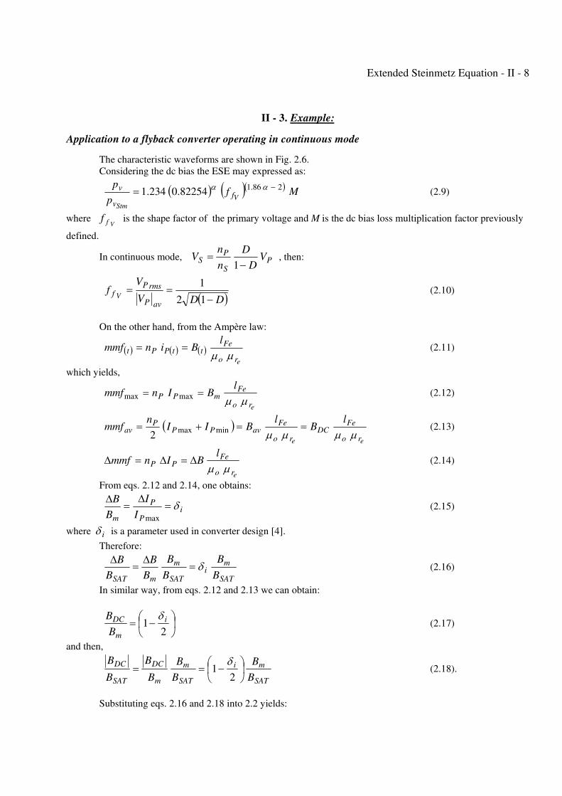
The characteristic waveforms are shown in Fig. 2.6.
Considering the dc bias the ESE may expressed as:
( ) ( )( )Mf
p
pV
Stm
fv
v 286.182254.0234.1
−= αα (2.9)
where Vff is the shape factor of the primary voltage and M is the dc bias loss multiplication factor previously
defined.
In continuous mode, PS
PS V
D
D
n
nV
−=
1, then:
( )DDV
Vf
avP
rmsPf V −
==12
1 (2.10)
On the other hand, from the Ampère law:
( ) ( ) ( )ero
FettPPt
lBinmmf
μμ== (2.11)
which yields,
ero
FemPP
lBInmmf
μμ== maxmax (2.12)
( )ee ro
FeDC
ro
FeavPP
Pav
lB
lBII
nmmf
μμμμ==+= minmax
2 (2.13)
ero
FePP
lBInmmf
μμΔ=Δ=Δ (2.14)
From eqs. 2.12 and 2.14, one obtains:
iP
P
m I
I
B
B δ=Δ
=Δ
max
(2.15)
where iδ is a parameter used in converter design [4].
Therefore:
SAT
mi
SAT
m
mSAT B
B
B
B
B
B
B
B δ=Δ=
Δ (2.16)
In similar way, from eqs. 2.12 and 2.13 we can obtain:
⎟⎠⎞
⎜⎝⎛ −=
21 i
m
DC
B
B δ (2.17)
and then,
SAT
mi
SAT
m
m
DC
SAT
DC
B
B
B
B
B
B
B
B⎟⎠
⎞⎜⎝
⎛ −==2
1δ
(2.18).
Substituting eqs. 2.16 and 2.18 into 2.2 yields:
Extended Steinmetz Equation - II - 9
SAT
mi
B
B
SAT
mi eB
BM
⎟⎠⎞
⎜⎝⎛−
⎟⎟⎠
⎞⎜⎜⎝
⎛⎟⎠
⎞⎜⎝
⎛ −+= 2
211
δξννδκ (2.19).
Substituting eqs. 2.10 and 2.19 into 2.9 yields:
( )( )[ ]( )
⎥⎥⎥
⎦
⎤
⎢⎢⎢
⎣
⎡
⎟⎟⎠
⎞⎜⎜⎝
⎛⎟⎠⎞
⎜⎝⎛ −+
−=
⎟⎠⎞
⎜⎝⎛−
−SAT
mi
Stm
B
B
SAT
mi
v
v eB
B
DDp
p 2
286.1 211
12
82254.0234.1
δξνν
α
α δκ (2.20).
Fig. 2.6 : Continuous operating mode flyback waveforms.
For a set of typical values D = 0.5 , α = 1.35 , Bm ≅ BSAT , δ i = 1/3 , κ = 7 , ν = 1.6 and ξ = 5 , one obtains:
1.3=Stmv
v
p
p, but in this expression
Stmvp corresponds to losses obtained for SATi BB δ=Δ , and so is
quite small compared to the losses in a transformer operating with mBB 2=Δ .
REFERENCES
[1] J.Reinert, A. Brockmeyer, and R.W. A. A. De Doncker, “Calculation of Losses in Ferro- and Ferrimagnetic Materials
Based on the Modified Steinmetz Equation”, IEEE Transactions on Industry Applications, vol. 37, no. 4, Jul./Aug. 2001.
[2] A. Brockmeyer, “Dimensionerungswerkzeug für magnetische Bauelemente in Stromritchteranwendungen”, Ph.D.
dissertation, Inst. Power Electron., Aachen, Germany, 1997.
[3] W. K. Mo, D. K. W. Cheng, and Y. S. Lee, “Simple Approximations of the DC Flux Influence on the Core Loss Power
Electronic Ferrites and Their Use in Design of Magnetic Components”, IEEE Transactions on Industrial Electronics, vol.44,
no. 6, Dec. 1997.
[4] H.E. Tacca, “Flyback vs. Forward Converter Topology Comparison Based upon Magnetic Design”, Eletrônica de
Potência , Vol. 5, no. 1, May 2000, Brazil.
t
t
T D T 0
mmf min
mmf av
mmf max
SS
P Vn
n−
PV
0
vp(t)
mmf(t)
Δmmf
Extended Steinmetz Equation - III - 1
PART III
MEASUREMENT TECHNIQUES
Extended Steinmetz Equation - III - 2
III - MEASUREMENT TECHNIQUES. PRINCIPLES
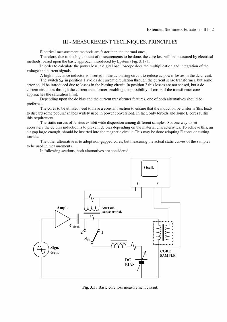
Electrical measurement methods are faster than the thermal ones.
Therefore, due to the big amount of measurements to be done, the core loss will be measured by electrical
methods, based upon the basic approach introduced by Epstein (Fig. 3.1) [1].
In order to calculate the power loss, a digital oscilloscope does the multiplication and integration of the
voltage and current signals.
A high inductance inductor is inserted in the dc biasing circuit to reduce ac power losses in the dc circuit.
The switch Sdc in position 1 avoids dc current circulation through the current sense transformer, but some
error could be introduced due to losses in the biasing circuit. In position 2 this losses are not sensed, but a dc
current circulates through the current transformer, enabling the possibility of errors if the transformer core
approaches the saturation limit.
Depending upon the dc bias and the current transformer features, one of both alternatives should be
preferred.
The cores to be utilized need to have a constant section to ensure that the induction be uniform (this leads
to discard some popular shapes widely used in power conversion). In fact, only toroids and some E cores fulfill
this requirement.
The static curves of ferrites exhibit wide dispersion among different samples. So, one way to set
accurately the dc bias induction is to prevent dc bias depending on the material characteristics. To achieve this, an
air gap large enough, should be inserted into the magnetic circuit. This may be done adopting E cores or cutting
toroids.
The other alternative is to adopt non-gapped cores, but measuring the actual static curves of the samples
to be used in measurements.
In following sections, both alternatives are considered.
Fig. 3.1 : Basic core loss measurement circuit.
current sense transf.
Sdc
2 1
Ampl.
Sign. Gen.
DC BIAS
Oscil.
i v
CORE SAMPLE
Cblock
Extended Steinmetz Equation - III - 3
REMARK: As the ferrite characteristics depend on the material temperature, the core samples under test are immersed in a bath of transformer oil heated at 100 oC. III - 1. MEASUREMENTS USING GAPPED CORES
Non-gapped E standard cores will be adopted and the air gap will be inserted in the central and
side legs using paper.
If the required air gap does not match any of the ones specified in manufacturer data sheets, the effective
permeability and inductance factor may be estimated using the formula presented in Appendix B.
Once the air gap is adopted, it is advisable to verify these calculated values before doing the experimental
measurements.
III - 1.1 Selection of the core volume
If the air gap fulfills rea ll μ>> , the effective permeability becomes:
ae
e
ar
rr ll
l
le≅
+=
μ
μμ
1
(3.1).
Then, adopting: ( )min
20 ra lel μ= , one obtains: 10020min
≅= rreμμ .
For the ferrite material 3C85 at 100 oC, from manufacturer data it is, 2000
min=rμ and
4400max
=rμ .
Therefore, this yields:
23.95min
=er
μ , 78.97max
=er
μ and 51.96=aver
μ .
Thus, the error due to relative permeability variation during measurements could be:
0264.0minmax =
−=
ave
ee
r
rr
reμ
μμμ , that is less than 3 %.
Therefore, air gaps yielding effective permeabilities of 100 (or less) should be adopted in order to keep
the error small.
On the other hand, from the Ampère law:
NA
SBI
L
Femm = (3.2)
where,
e
Fero
Ll
SA e
μμ= (3.3)
and from the Faraday law:
fSB
VN
Fem
P
44.4= (3.4).
Substituting eqs. 3.3 and 3.4 into eq. 3.2 yields:
Pro
mm
V
fVolBI
eμμ
244.4
= (3.5)
Extended Steinmetz Equation - III - 4
where, eFe lSVol = .
From eq. 3.5 one may obtains the required core volume as function of the maximum current to be
supplied by the driving amplifier:
fB
IVVol
m
mPro e
244.4
μμ= (3.6).
Considering IIm 2= , the eq. 3.6 becomes:
fB
PVol
m
ampro e
2π
μμ= (3.7)
where ampP is the required amplifier nominal output power.
Examples
For f = 20 kHz , Bm = 0.3 T , 100=er
μ and WPamp 250= , it results: 3mm5555=Vol .
The core E42/21/15 has a volume of 17300 mm3 , so it is too big for the amplifier power available. This
may be also verified using eqs. 3.2 and 3.4:
1. From eq. 3.4 : 2109.21 ≅=N .
2. From manufacturer data one may adopt 110=er
μ which yields nH250=LA . Then, adopting VP = 100 V ,
eq. 3.2 yields: AANA
SBI
L
Femm 17.10
2110250
101783.09
6
=×
×==
−
−.
If an error of 5 % were acceptable, one may adopt 270=er
μ , giving nH630=LA which yields A4=mI
.
For f = 100 kHz, one may raise the induction up to Bm = 0.2 T and then, from eq. 3.4 : 6326.6 ≅=N .
Later, adopting 270=er
μ the eq. 3.2 yields: A42.9=mI .
From results above obtained from eq. 3.7 , one possibility to measure the losses using the available
amplifier of 250 W, might be to adopt cores EF25 (E25/13/7) having 3mm2990=Vol .
This was the core size adopted to do the experimental measurements.
III - 1.2 Minimum required window filling factor
The rms current through the windings is:
NA
SBI
L
Femrms
2
1= (3.8).
On the other hand:
N
SFFFSI Fe
wcpCurms σσ == (3.9)
where,
σ : current density
pF : partition factor of the window
cF : coil factor (or filling factor)
Extended Steinmetz Equation - III - 5
wF : window factor , Feww SSF =
Substituting eq. 3.9 into eq. 3.8 yields:
pwL
mc
FFA
BF
σ1
2
1min
= (3.10).
Thus , the filling factor should be equal or better than the limit given by eq. 3.10 .
For the cores E25/13/7 made with material 3C85, from manufacturer data the air gap should be 270 μm in
order to set LA with accuracy + - 3 % . Adopting such air gap (but sharing it between the external and central
legs), it results %1.3240 ±=LA .
For TBm 3.0= , 2/5.4 mmA=σ , 077.1=wF , and 9.0=pF the minimum filling factor
results: 203.0min
=cF . This requirement may not be fulfilled using cable winding, because the window filling
factor using cable typically ranges from 0.07 to 0.09 .
Using other cores the situation does not change much. For example , for E42-15 the minimum filling
factor is 0.155 .
For a core E55-21, adopting 2/5.4 mmA=σ and 95.0=pF , it results 9.0
min=cF . Then, from
eq. 3.8 it should be AI rms 96.3= , but for this current and an environment temperature of 100 oC, it may be
not safe to adopt such current density. (Lowering the current density will raise the minimum required filling
factor).
Therefore, wire windings should be used. Moreover, the amount of winding space required will not allow
to use isolated windings for ac driving primary and dc biasing windings.
III - 1.3 Instrument accuracy requirements
The averaged product of signals from channels 1 and 2 has usually an offset, which may change with the
repetition of the measurement and with the number of averaging cycles. Also, it varies when the voltage/division
rate is modified.
However, a simple way to correct for offset errors is to do two measurements (W1 and W2), inverting the
connection of the voltage sense winding without changing the voltage/div ratios. As the offset error should remain
the same, the expression ( ) 2/21 WWW −= allows eliminating offset errors.
Unfortunately, this did not solve the accuracy problems.
Using a non-gapped core E25/13/7 made on material 3C85 , adopting Bm = 0.2 T and f = 25 kHz , the
apparent power was 0.705 W , while the active power was 35 mW. That is, the ratio of the wanted average to the
apparent instantaneous power to be averaged was FP = 0.05 (the power factor).
On the other hand, in the case of the gapped core, the power factor results: FP = 0.0045, so one order of
magnitude lower.
Then to have a precision of %5.2± on the result, a resolution of FP/40 in the signal product is
required, that is FP/40 = 0.0001125 , which leads to a required precision of 0106.040/ =FP for the input
signals. As the input signals may be usually ranging on the medium voltage span (selected by the voltage/div
control) this ask for a 0.5 % class requirement for the input channels.
Moreover, the signal multiplication must have a 0.0001 resolution, which implies 14 bits. Actually, for
signals ranging on the medium voltage span, the required resolution is 0.00005. Therefore, two bytes operation
and register are needed.
Increasing the core volume, or using multiple cores in parallel, will not change the situation because the
apparent power would be increased in the same proportion (both the active power and the apparent power are
proportional to the core volume).
Extended Steinmetz Equation - III - 6
When using a non-gapped core the precision required becomes much lower due to the apparent power
reduction.
If curves corresponding to small loss operation are to be plotted, the instrument accuracy demands may be
impossible to meet when using gapped cores [2].
III - 2. MEASUREMENTS USING NON-GAPPED CORES
In ferrites the static B-H curve matches the low frequency normal curve [3] which allows to use this
normal curve to find the dc currents to be injected.
Using a non-gapped core, for a given induction Bm it will be a maximum Hm related to a peak current Im
by the Ampère law.
Assuming the normal curve equal to the static one, injecting Idc = Im should produce Bdc = Bm.
Therefore, to find the dc current to be injected one should apply an ac voltage producing a Bm equal to
the desired Bdc , then measure Im and so finally inject Idc = Im.
The normal curve differs from the static curve as much as the core eddy currents become important. Thus,
to obtain a good Idc prediction, one should use a low frequency normal curve, for example at 1 kHz.
This may be accomplished using two sets of windings, one having more turns to find Idc and other with
few turns to measure losses.
In order to avoid resonance problems while doing high frequency measurements, a set of two coil formers
should be foresee.
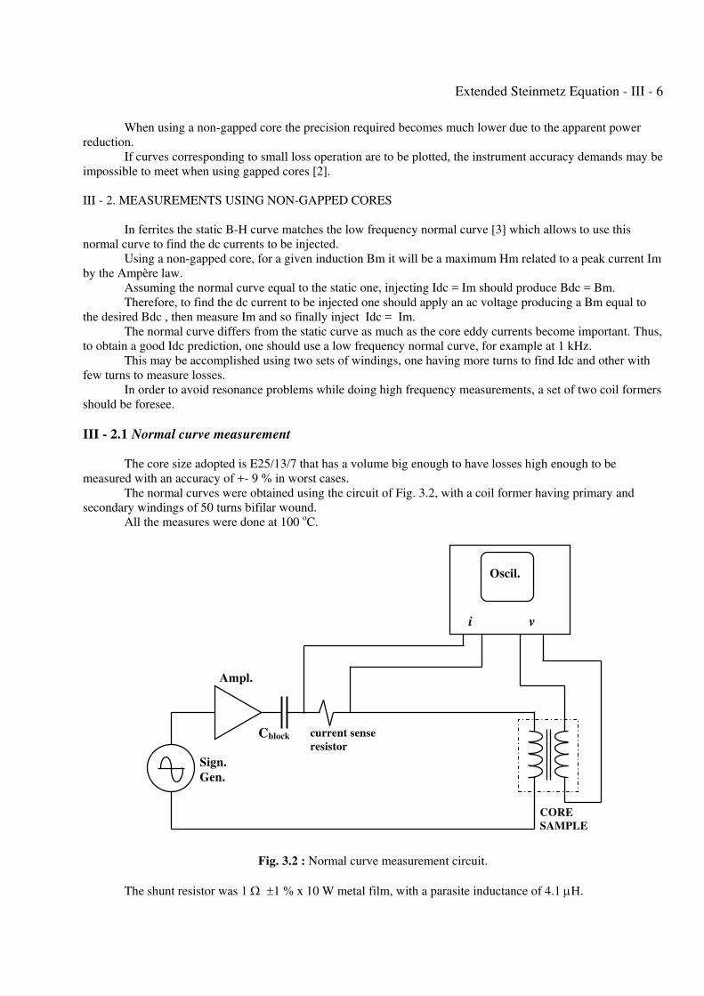
III - 2.1 Normal curve measurement
The core size adopted is E25/13/7 that has a volume big enough to have losses high enough to be
measured with an accuracy of +- 9 % in worst cases.
The normal curves were obtained using the circuit of Fig. 3.2, with a coil former having primary and
secondary windings of 50 turns bifilar wound.
All the measures were done at 100 oC.
Fig. 3.2 : Normal curve measurement circuit.
The shunt resistor was 1 Ω ±1 % x 10 W metal film, with a parasite inductance of 4.1 μH.
current sense resistor
Ampl.
Sign. Gen.
Oscil.
i v
CORE SAMPLE
Cblock
Extended Steinmetz Equation - III - 7
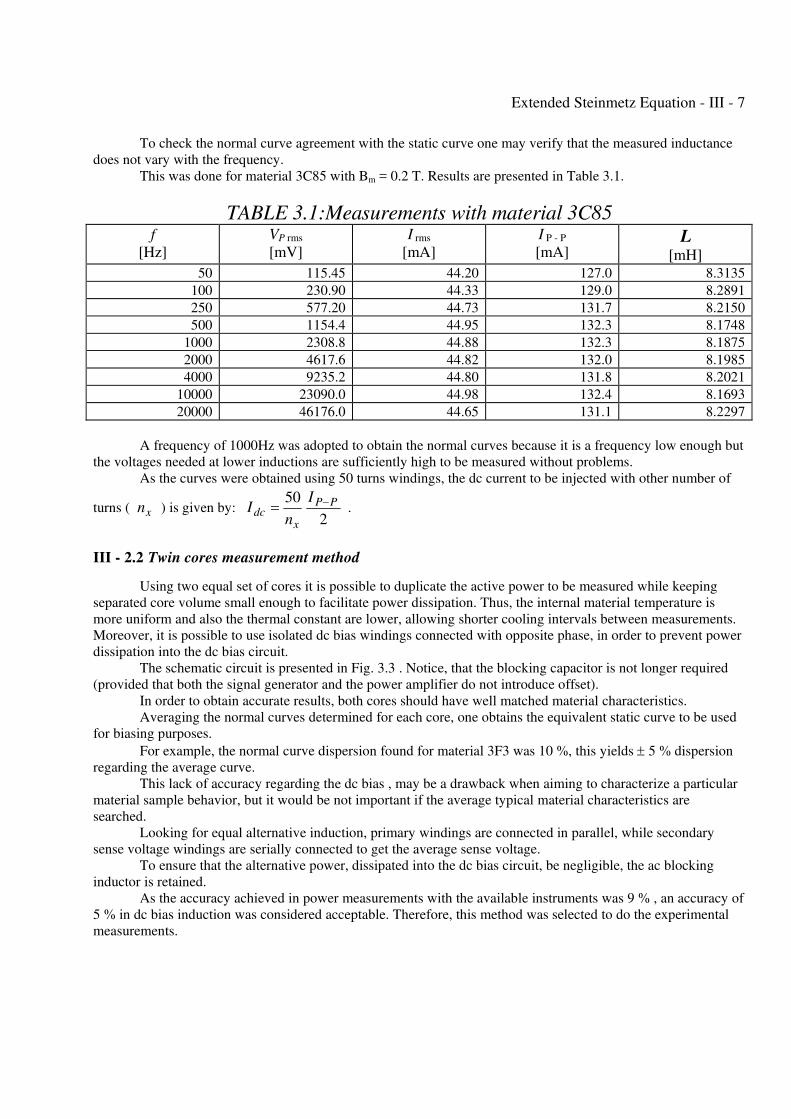
To check the normal curve agreement with the static curve one may verify that the measured inductance
does not vary with the frequency.
This was done for material 3C85 with Bm = 0.2 T. Results are presented in Table 3.1.
TABLE 3.1:Measurements with material 3C85 f
[Hz]
VP rms
[mV]
I rms
[mA]
I P - P
[mA] L
[mH] 50 115.45 44.20 127.0 8.3135
100 230.90 44.33 129.0 8.2891
250 577.20 44.73 131.7 8.2150
500 1154.4 44.95 132.3 8.1748
1000 2308.8 44.88 132.3 8.1875
2000 4617.6 44.82 132.0 8.1985
4000 9235.2 44.80 131.8 8.2021
10000 23090.0 44.98 132.4 8.1693
20000 46176.0 44.65 131.1 8.2297
A frequency of 1000Hz was adopted to obtain the normal curves because it is a frequency low enough but
the voltages needed at lower inductions are sufficiently high to be measured without problems.
As the curves were obtained using 50 turns windings, the dc current to be injected with other number of
turns ( xn ) is given by: 2
50 PP
xdc
I
nI −= .
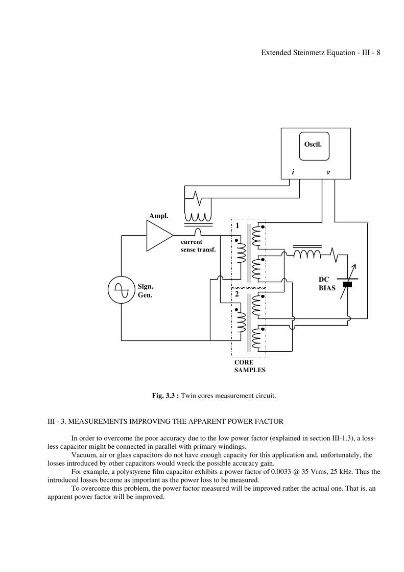
III - 2.2 Twin cores measurement method
Using two equal set of cores it is possible to duplicate the active power to be measured while keeping
separated core volume small enough to facilitate power dissipation. Thus, the internal material temperature is
more uniform and also the thermal constant are lower, allowing shorter cooling intervals between measurements.
Moreover, it is possible to use isolated dc bias windings connected with opposite phase, in order to prevent power
dissipation into the dc bias circuit.
The schematic circuit is presented in Fig. 3.3 . Notice, that the blocking capacitor is not longer required
(provided that both the signal generator and the power amplifier do not introduce offset).
In order to obtain accurate results, both cores should have well matched material characteristics.
Averaging the normal curves determined for each core, one obtains the equivalent static curve to be used
for biasing purposes.
For example, the normal curve dispersion found for material 3F3 was 10 %, this yields ± 5 % dispersion
regarding the average curve.
This lack of accuracy regarding the dc bias , may be a drawback when aiming to characterize a particular
material sample behavior, but it would be not important if the average typical material characteristics are
searched.
Looking for equal alternative induction, primary windings are connected in parallel, while secondary
sense voltage windings are serially connected to get the average sense voltage.
To ensure that the alternative power, dissipated into the dc bias circuit, be negligible, the ac blocking
inductor is retained.
As the accuracy achieved in power measurements with the available instruments was 9 % , an accuracy of
5 % in dc bias induction was considered acceptable. Therefore, this method was selected to do the experimental
measurements.
Extended Steinmetz Equation - III - 8
Fig. 3.3 : Twin cores measurement circuit.
III - 3. MEASUREMENTS IMPROVING THE APPARENT POWER FACTOR
In order to overcome the poor accuracy due to the low power factor (explained in section III-1.3), a loss-
less capacitor might be connected in parallel with primary windings.
Vacuum, air or glass capacitors do not have enough capacity for this application and, unfortunately, the
losses introduced by other capacitors would wreck the possible accuracy gain.
For example, a polystyrene film capacitor exhibits a power factor of 0.0033 @ 35 Vrms, 25 kHz. Thus the
introduced losses become as important as the power loss to be measured.
To overcome this problem, the power factor measured will be improved rather the actual one. That is, an
apparent power factor will be improved.
current sense transf.
2
1
Ampl.
Sign. Gen.
DC BIAS
Oscil.
i v
CORE SAMPLES
Extended Steinmetz Equation - III - 9
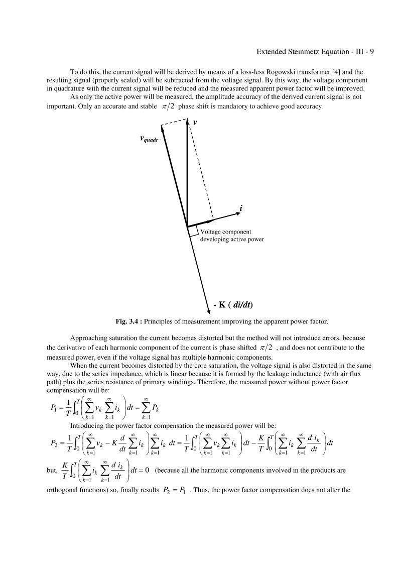
To do this, the current signal will be derived by means of a loss-less Rogowski transformer [4] and the
resulting signal (properly scaled) will be subtracted from the voltage signal. By this way, the voltage component
in quadrature with the current signal will be reduced and the measured apparent power factor will be improved.
As only the active power will be measured, the amplitude accuracy of the derived current signal is not
important. Only an accurate and stable 2π phase shift is mandatory to achieve good accuracy.
Fig. 3.4 : Principles of measurement improving the apparent power factor.
Approaching saturation the current becomes distorted but the method will not introduce errors, because
the derivative of each harmonic component of the current is phase shifted 2π , and does not contribute to the
measured power, even if the voltage signal has multiple harmonic components.
When the current becomes distorted by the core saturation, the voltage signal is also distorted in the same
way, due to the series impedance, which is linear because it is formed by the leakage inductance (with air flux
path) plus the series resistance of primary windings. Therefore, the measured power without power factor
compensation will be:
∑∫ ∑∑∞
=
∞
=
∞
=
=⎟⎟⎠
⎞⎜⎜⎝
⎛=
10
11
1
1
k
k
T
k
k
k
k PdtivT
P
Introducing the power factor compensation the measured power will be:
dtdt
idi
T
Kdtiv
Tdtii
dt
dKv
TP
T
k
k
k
k
T
k
k
k
k
k
k
T
k
k
k
k ∫ ∑∑∫ ∑∑∑∫ ∑∑ ⎟⎟⎠
⎞⎜⎜⎝
⎛−⎟
⎟⎠
⎞⎜⎜⎝
⎛=⎟
⎟⎠
⎞⎜⎜⎝
⎛−=
∞
=
∞
=
∞
=
∞
=
∞
=
∞
=
∞
=0
110
1110
11
2
11
but, 00
11
=⎟⎟⎠
⎞⎜⎜⎝
⎛∫ ∑∑
∞
=
∞
=
dtdt
idi
T
K T
k
k
k
k (because all the harmonic components involved in the products are
orthogonal functions) so, finally results 12 PP = . Thus, the power factor compensation does not alter the
i
- K ( di/dt)
v
vquadr
Voltage component
developing active power
Extended Steinmetz Equation - III - 10
measured power. Moreover, this might allow using this measurement improvement technique with non sinusoidal
waveforms.
The most promising feature of this method is that it might allow testing components having large air gaps.
In order to test the derivative performance, one Rogowski transformer was assembled winding two
Rogowski coils on the same toroidal air core. The derived current signal matched quite well the digital derivative
done by the digital oscilloscope.
The use of a Rogowski transformer instead of a single Rogowski coil allows overcoming the poor
sensitivity of the single coil for small currents. Moreover, the flux is better confined inside the toroid giving both
a more stable signal and higher noise immunity.
Further exploration of this proposed technique will be done in future works.
III - 4. CONCLUSIONS AND FUTURE WORK
1. From the experimental measurements done, one may conclude that for the particular case of flyback
converters operating in discontinuous mode at low frequency (i.e. 25 kHz) and designed for minimum core
volume, the classical Steinmetz equation may be applied for transformer design. This is possible because in such
cases the design is limited by saturation and also, the dc bias is usually lower than half of the maximum induction
attained.
In such conditions the core losses are smaller or hardly bigger than the ones corresponding to the
unbiased condition. Moreover, as the duty factor is usually adopted near 50 % , the non sinusoidal waveform does
not significatively affect losses so, using ESE or iGSE might not be necessary.
2. If a flyback transformer has to be optimized from the efficiency point of view (minimizing losses) the
optimal maximum induction should be reduced [5]. In this case, the dc bias may increase the losses with respect
to the classical Steinmetz results.
3. If an asymmetrical converter has to operate at high frequency, the maximum allowable induction is
limited by losses at values that exhibit great variations depending upon the bias adopted. In this case the dc bias
will have a strong influence in transformer design. This will be true in the particular case of quasi-resonant
converters, where the switching frequency adopted is the highest possible, but the goal is to reach very high
efficiencies.
4. In order to test the loss prediction models many samples from different materials need to be characterized
varying frequency, maximum alternative induction, dc bias and eventually temperature. This requires such a large
number of measurements that some form of automatic instrument should be developed.
A B-H analyzer capable of measuring losses using the most common waveforms in power electronics
might be developed as a student project. The default waveform operation should be sinewave and the power factor
compensation should be included as selectable function.
5. The dc bias and non-sinusoidal waveform influence may be considered using different approaches based
upon sinewave made measurements. This suggest that a convenient way for the manufacturers to specify their
products is to give the family of curves plotted with sinusoidal drive under dc bias conditions. To obtain these
families of curves many samples of each material should be measured in order to get the average results.
Again, this would be only feasible having an automatic measurement system.
6. As future work, the joint application of the models dealing with both minor loops and dc bias will be used
to calculate the core losses in power factor corrector circuits.
Extended Steinmetz Equation - III - 11
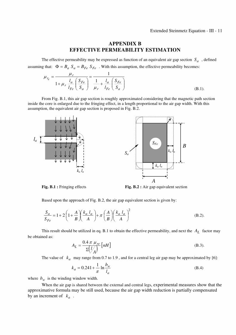
APPENDIX B EFFECTIVE PERMEABILITY ESTIMATION
The effective permeability may be expressed as function of an equivalent air gap section aS , defined
assuming that: FeFeaa SBSB ==Φ . With this assumption, the effective permeability becomes:
⎟⎟⎠
⎞⎜⎜⎝
⎛+
=
⎟⎟⎠
⎞⎜⎜⎝
⎛+
=
a
Fe
Fe
a
ra
Fe
Fe
ar
rr
S
S
l
l
S
S
l
le
μμ
μμ
1
1
1 (B.1).
From Fig. B.1, this air gap section is roughly approximated considering that the magnetic path section
inside the core is enlarged due to the fringing effect, in a length proportional to the air gap width. With this
assumption, the equivalent air gap section is proposed in Fig. B.2.
Fig. B.1 : Fringing effects Fig. B.2 : Air gap equivalent section
Based upon the approach of Fig. B.2, the air gap equivalent section is given by:
2
121 ⎟⎠
⎞⎜⎝
⎛⎟⎠⎞
⎜⎝⎛+⎟
⎠
⎞⎜⎝
⎛⎟⎠⎞
⎜⎝⎛ ++=
A
lk
B
A
A
lk
B
A
S
S aaaa
Fe
a π (B.2).
This result should be utilized in eq. B.1 to obtain the effective permeability, and next the LA factor may
be obtained as:
( ) [ ]nH
Al
A reL
Σ=
μπ4.0 (B.3).
The value of ak may range from 0.7 to 1.9 , and for a central leg air gap may be approximated by [6]:
a
wa
l
bk ln
1241.0
π+= (B.4)
where wb is the winding window width.
When the air gap is shared between the external and central legs, experimental measures show that the
approximative formula may be still used, because the air gap width reduction is partially compensated
by an increment of ak .
la
ka la
A
B
SFe
Sa ka la
ka la
Extended Steinmetz Equation - III - 12
REFERENCES
[1] S.-C Wang and C.-L. Chen, “PC-based apparatus for characterising high frequency magnetic cores”, IEE Proc. - Sci.
Meas. Technology , Vol. 146, no. 6, U.K., Nov. 1999.
[2] R. Linkous, A. W. Kelley, and K. C. Armstrong, “An improved calorimeter for measuring the core loss of magnetic
materials”, Applied Power Electronics Conf. and Expo. 2000 (IEEE - APEC 2000).
[3] G. Bertotti, “Hysteresis in magnetism”, Academic Press, 1998, (Chap. 1 - Sect. 1.2).
[4] G. D’Antona et al., “AC measurements via digital processing of Rogowski coils signal”, IEEE Instrumentation and
Measurement Technology Conference , Anchorage, USA, May 2002.
[5] H.E. Tacca, “Flyback vs. Forward Converter Topology Comparison Based upon Magnetic Design”, Eletrônica de
Potência , Vol. 5, no. 1, May 2000, Brazil.
[6] E. C. Snelling, “Soft Ferrites: Properties and Applications”, Butterworths, U.K., 1988 (Chap. 4 - Sect. 4.2.2).
Appendix C - 1
APPENDIX C
EXPERIMENTAL RESULTS
Appendix C - 2
Bm [T]
VOLTAGE [Vrms]
(50 turns) I rms I p-p [mA] [mA]
(5 turns) I dc
[mA]
0.025 0.2886 5.78 15.66 78.30
0.05 0.5772 11.70 33.24 166.20
0.1 1.1544 22.40 64.10 320.50
0.15 1.7316 33.50 97.00 485.00
0.2 2.3088 44.84 132.30 661.50
0.25 2.8860 58.10
175.20
876.00
0.3 3.4632 75.00
240.00
1200.00
NORMAL CURVE
Material: 3C85 Ferroxcube
Frequency: 1 kHz
Appendix C - 3
Bac [T] Bdc [T]
0.025 0.05 0.1 0.15 0.2 0.25 0.3
0.0 1.260
1.350
1.340
6.770
6.900
7.000
35.900
35.700
36.100
99.500
100.000
101.500
200.000
203.600
209.000
344.000
342.000
527.000
525.000
518.000
0.025 1.210
1.200
6.710
6.690
35.900
36.300
99.000
100.700
203.000
205.000
342.000
344.000
524.000
521.000
0.05 1.180
1.250
6.600
6.590
36.800
36.500
100.000
102.000
203.800
207.000
339.600
337.500
341.000
0.1 1.360
1.314
7.820
7.840
41.700
42.100
106.400
107.000
111.000
216.000
217.500
345.000
347.000
348.500
0.15 1.640
1.620
10.340
9.700
52.500
51.900
120.200
120.700
123.000
224.000
229.000
0.2 2.570
2.500
14.100
13.380
66.500
66.100
130.600
130.850
0.25 3.900
3.780
19.780
20.050
19.560
80.300
80.200
0.3 7.220
7.120
30.100
29.530
CORE LOSS [mW] CORE: E/25/13/7
MATERIAL: 3C85 Ferroxcube
FREQUENCY: 25 kHz
AC WINDINGS: 5 turns SAT
SAT
SAT
SAT
SAT
Appendix C - 4
Bac [T] Bdc [T]
0.025 0.05 0.1 0.15 0.2 0.25 0.3
0.0 2.150
2.180
14.590
14.290
14.440
78.100
77.150
228.500
228.750
476.620
474.300
477.000
826.620
823.620
1277.000
1275.620
0.025 2.050
1.980
14.250
14.300
76.650
76.990
227.750
227.350
474.250
471.330
818.870
824.500
1271.000
1272.870
0.05 2.040
1.940
14.520
14.420
77.910
78.680
227.870
228.370
475.000
475.620
821.620
819.620
1267.250
1265.120
0.1 2.250
2.150
16.790
16.730
88.920
89.210
247.000
246.120
498.870
499.120
838.000
842.870
846.370
841.250
1277.620
1276.620
1275.870
0.15 2.500
2.460
21.020
20.770
109.110
108.350
278.870
279.620
534.120
533.750
870.370
867.250
0.2 3.750
3.720
27.080
26.810
133.000
132.000
315.750
312.750
0.25 6.050
5.950
36.300
35.900
159.620
159.750
0.3 10.200
10.100
47.190
47.120
CORE LOSS [mW] CORE: E/25/13/7
MATERIAL: 3C85 Ferroxcube
FREQUENCY: 50 kHz
AC WINDINGS: 5 turns
SAT
SAT
SAT
SAT
Appendix C - 5
Bac [T] Bdc [T]
0.025 0.05 0.1 0.15 0.2 0.25 0.3
0.0 5.490
6.060
5.340
5.980
38.290
36.620
35.800
35.550
222.120
220.620
220.870
606.620
609.750
608.750
611.370
1277.620
1297.250
1289.000
2230.870
2245.500
2238.500
3480.000
3451.250
3462.500
0.025 5.580
5.590
5.660
36.250
36.150
36.110
219.250
220.500
220.000
610.250
604.750
605.120
1288.870
1282.870
1291.750
2230.250
2228.120
2232.290
0.05 5.640
5.520
5.590
36.640
36.220
36.210
222.370
222.500
221.370
607.620
614.250
614.250
1294.370
1288.870
1286.000
2229.370
2232.750
2238.500
0.1 6.000
5.850
5.820
41.670
41.290
40.900
248.250
248.120
249.000
661.500
659.870
656.000
1345.750
1341.250
1339.000
2273.370
2261.750
2270.870
0.15 7.740
7.410
7.390
52.500
52.450
52.290
286.120
286.120
284.120
739.000
739.120
737.750
1414.620
1418.370
1417.250
2313.750
2307.500
0.2 9.560
9.700
9.740
68.190
68.430
68.020
348.620
347.370
347.120
818.500
817.370
817.500
1474.500
1474.100
0.25 15.460
15.770
15.710
94.350
94.290
94.020
411.120
412.620
411.370
893.620
892.620
896.370
0.3 28.240
28.010
28.050
101.840
102.720
102.620
486.750
486.870
484.870
CORE LOSS [mW] CORE: E/25/13/7
MATERIAL: 3C85 Ferroxcube
FREQUENCY: 100 kHz
AC WINDINGS: 5 turns
SAT
SAT
T ≠ Cnt
T ≠ Cnt
SAT
SAT
Appendix C - 6
Bac [T] Bdc [T]
0.025 0.05 0.1 0.15
(5 turns)
0.2
(2 turns)
0.25 0.3
0.0 19.590
19.520
19.550
120.910
120.310
119.760
668.000
666.620
668.000
1871.000
1874.750
1875.000
4056.250
4083.750
4022.500
4108.750
0.025 19.620
19.420
19.400
118.200
118.040
117.620
666.620
664.750
666.250
1870.750
1868.870
1871.120
4026.250
4037.500
3950.000
0.05 20.170
20.000
20.040
119.610
118.650
119.950
664.000
661.000
660.500
1880.500
1884.870
1883.750
3995.000
3997.500
4023.700
0.1 22.670
22.270
22.220
133.690
132.270
131.610
725.500
725.620
725.370
2002.870
2003.250
1997.370
4025.000
4133.700
4165.000
0.15 26.070
26.000
26.160
165.200
164.120
163.390
874.500
872.370
872.250
2222.370
2213.750
2217.250
4177.500
4223.700
4267.500
0.2 31.750
31.470
31.950
212.750
211.750
210.750
1044.620
1044.850
1045.500
2443.120
2464.370
2427.120
4371.250
4372.500
4413.750
0.25 45.860
47.370
47.100
276.750
276.120
276.500
1185.880
1197.500
1202.500
0.3 75.640
74.500
74.000
338.620
330.370
326.630
1273.000
1272.250
CORE LOSS [mW] CORE: E/25/13/7
MATERIAL: 3C85 Ferroxcube
FREQUENCY: 200 kHz
AC WINDINGS: 5 and 2 turns
SATSAT
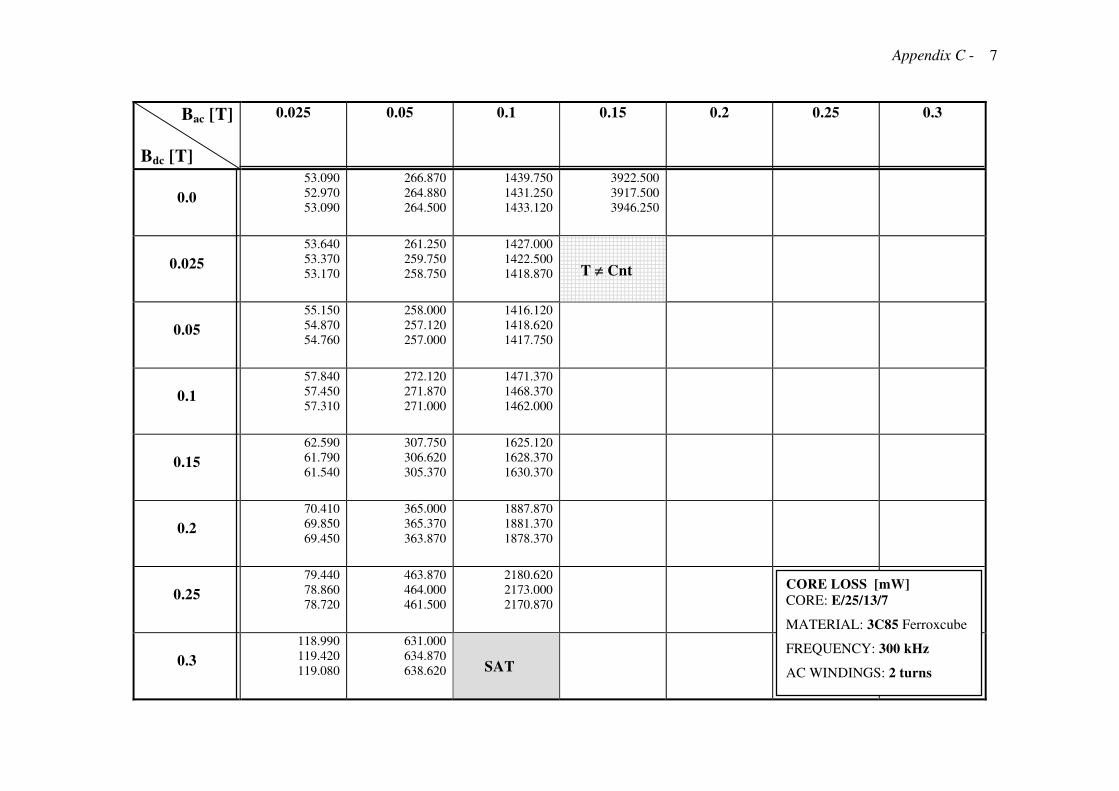
Appendix C - 7
Bac [T] Bdc [T]
0.025 0.05 0.1 0.15 0.2 0.25 0.3
0.0 53.090
52.970
53.090
266.870
264.880
264.500
1439.750
1431.250
1433.120
3922.500
3917.500
3946.250
0.025 53.640
53.370
53.170
261.250
259.750
258.750
1427.000
1422.500
1418.870
0.05 55.150
54.870
54.760
258.000
257.120
257.000
1416.120
1418.620
1417.750
0.1 57.840
57.450
57.310
272.120
271.870
271.000
1471.370
1468.370
1462.000
0.15 62.590
61.790
61.540
307.750
306.620
305.370
1625.120
1628.370
1630.370
0.2 70.410
69.850
69.450
365.000
365.370
363.870
1887.870
1881.370
1878.370
0.25 79.440
78.860
78.720
463.870
464.000
461.500
2180.620
2173.000
2170.870
0.3 118.990
119.420
119.080
631.000
634.870
638.620
CORE LOSS [mW] CORE: E/25/13/7
MATERIAL: 3C85 Ferroxcube
FREQUENCY: 300 kHz
AC WINDINGS: 2 turns SAT
T ≠ Cnt
Appendix C - 8
Bm [T]
VOLTAGE
[Vrms]
I p-p (50 turns) [mA]
(5 turns) I dc
[mA]
0.025 0.2886 21.06
19.50
101
0.05 0.5772 41.43 38.16 199
0.1 1.1544 80.60 73.32 385
0.15 1.7316 119.60 110.90 576
0.2 2.3088 161.10 148.40 774
0.25 2.8860 206.00 191.40 994
0.3 3.4632 263.80 246.40 1276
NORMAL CURVE
Material: 3F3 Ferroxcube
Frequency: 1 kHz ( DC induction bias error < ± 5 % )
core # 1 core # 2
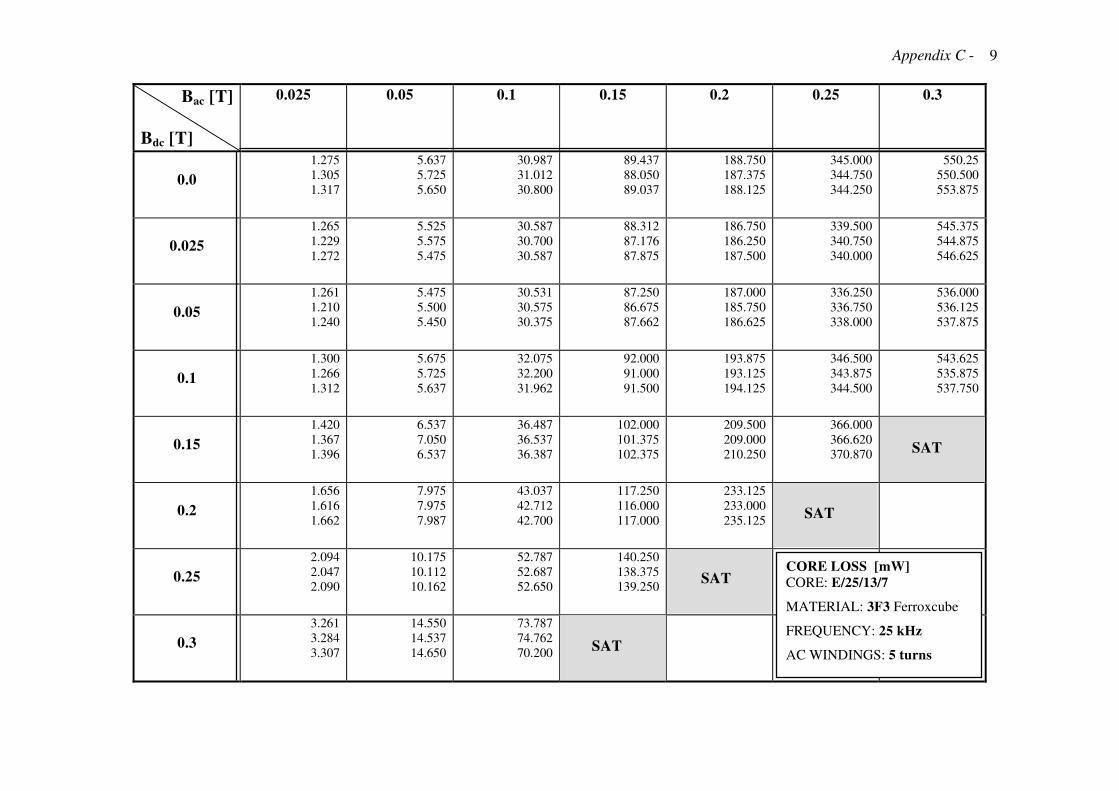
Appendix C - 9
Bac [T] Bdc [T]
0.025 0.05 0.1 0.15 0.2 0.25 0.3
0.0 1.275
1.305
1.317
5.637
5.725
5.650
30.987
31.012
30.800
89.437
88.050
89.037
188.750
187.375
188.125
345.000
344.750
344.250
550.25
550.500
553.875
0.025 1.265
1.229
1.272
5.525
5.575
5.475
30.587
30.700
30.587
88.312
87.176
87.875
186.750
186.250
187.500
339.500
340.750
340.000
545.375
544.875
546.625
0.05 1.261
1.210
1.240
5.475
5.500
5.450
30.531
30.575
30.375
87.250
86.675
87.662
187.000
185.750
186.625
336.250
336.750
338.000
536.000
536.125
537.875
0.1 1.300
1.266
1.312
5.675
5.725
5.637
32.075
32.200
31.962
92.000
91.000
91.500
193.875
193.125
194.125
346.500
343.875
344.500
543.625
535.875
537.750
0.15 1.420
1.367
1.396
6.537
7.050
6.537
36.487
36.537
36.387
102.000
101.375
102.375
209.500
209.000
210.250
366.000
366.620
370.870
0.2 1.656
1.616
1.662
7.975
7.975
7.987
43.037
42.712
42.700
117.250
116.000
117.000
233.125
233.000
235.125
0.25 2.094
2.047
2.090
10.175
10.112
10.162
52.787
52.687
52.650
140.250
138.375
139.250
0.3 3.261
3.284
3.307
14.550
14.537
14.650
73.787
74.762
70.200
CORE LOSS [mW] CORE: E/25/13/7
MATERIAL: 3F3 Ferroxcube
FREQUENCY: 25 kHz
AC WINDINGS: 5 turns
SAT
SAT
SAT
SAT
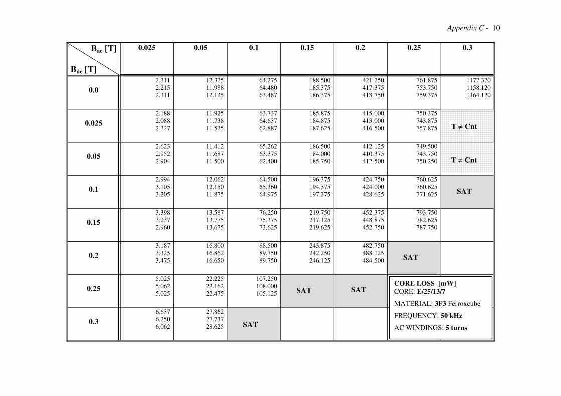
Appendix C - 10
Bac [T] Bdc [T]
0.025 0.05 0.1 0.15 0.2 0.25 0.3
0.0 2.311
2.215
2.311
12.325
11.988
12.125
64.275
64.480
63.487
188.500
185.375
186.375
421.250
417.375
418.750
761.875
753.750
759.375
1177.370
1158.120
1164.120
0.025 2.188
2.088
2.327
11.925
11.738
11.525
63.737
64.637
62.887
185.875
184.875
187.625
415.000
413.000
416.500
750.375
743.875
757.875
0.05 2.623
2.952
2.904
11.412
11.687
11.500
65.262
63.375
62.400
186.500
184.000
185.750
412.125
410.375
412.500
749.500
743.750
750.250
0.1 2.994
3.105
3.205
12.062
12.150
11.875
64.500
65.360
64.975
196.375
194.375
197.375
424.750
424.000
428.625
760.625
760.625
771.625
0.15 3.398
3.237
2.960
13.587
13.775
13.675
76.250
75.375
73.625
219.750
217.125
219.625
452.375
448.875
452.750
793.750
782.625
787.750
0.2 3.187
3.325
3.475
16.800
16.862
16.650
88.500
89.750
89.750
243.875
242.250
246.125
482.750
488.125
484.500
0.25 5.025
5.062
5.025
22.225
22.162
22.475
107.250
108.000
105.125
0.3 6.637
6.250
6.062
27.862
27.737
28.625
CORE LOSS [mW] CORE: E/25/13/7
MATERIAL: 3F3 Ferroxcube
FREQUENCY: 50 kHz
AC WINDINGS: 5 turns
SAT
SAT
SAT
SAT
SAT
T ≠ Cnt
T ≠ Cnt
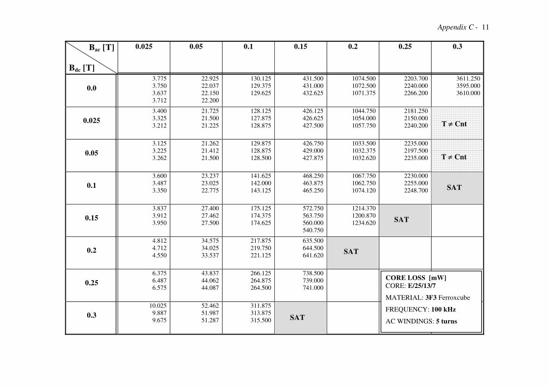
Appendix C - 11
Bac [T] Bdc [T]
0.025 0.05 0.1 0.15 0.2 0.25 0.3
0.0 3.775
3.750
3.637
3.712
22.925
22.037
22.150
22.200
130.125
129.375
129.625
431.500
431.000
432.625
1074.500
1072.500
1071.375
2203.700
2240.000
2266.200
3611.250
3595.000
3610.000
0.025 3.400
3.325
3.212
21.725
21.500
21.225
128.125
127.875
128.875
426.125
426.625
427.500
1044.750
1054.000
1057.750
2181.250
2150.000
2240.200
0.05 3.125
3.225
3.262
21.262
21.412
21.500
129.875
128.875
128.500
426.750
429.000
427.875
1033.500
1032.375
1032.620
2235.000
2197.500
2235.000
0.1 3.600
3.487
3.350
23.237
23.025
22.775
141.625
142.000
143.125
468.250
463.875
465.250
1067.750
1062.750
1074.120
2230.000
2255.000
2248.700
0.15 3.837
3.912
3.950
27.400
27.462
27.500
175.125
174.375
174.625
572.750
563.750
560.000
540.750
1214.370
1200.870
1234.620
0.2 4.812
4.712
4.550
34.575
34.025
33.537
217.875
219.750
221.125
635.500
644.500
641.620
0.25 6.375
6.487
6.575
43.837
44.062
44.087
266.125
264.875
264.500
738.500
739.000
741.000
0.3 10.025
9.887
9.675
52.462
51.987
51.287
311.875
313.875
315.500
CORE LOSS [mW] CORE: E/25/13/7
MATERIAL: 3F3 Ferroxcube
FREQUENCY: 100 kHz
AC WINDINGS: 5 turns
SAT
SAT
SAT
SAT
T ≠ Cnt
T ≠ Cnt
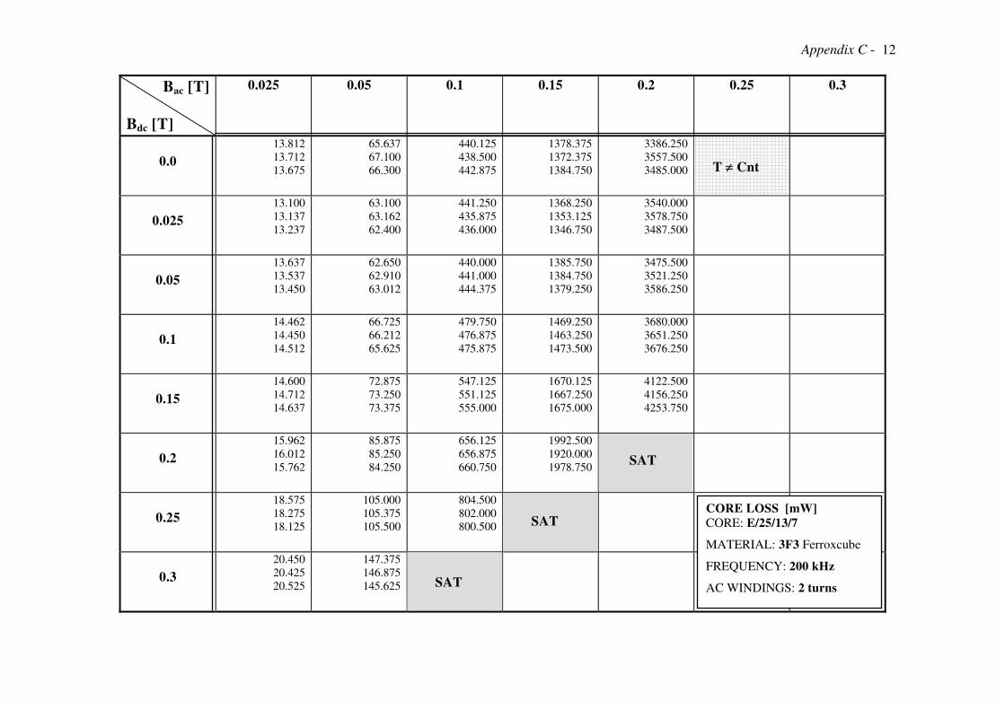
Appendix C - 12
Bac [T] Bdc [T]
0.025 0.05 0.1 0.15 0.2 0.25 0.3
0.0 13.812
13.712
13.675
65.637
67.100
66.300
440.125
438.500
442.875
1378.375
1372.375
1384.750
3386.250
3557.500
3485.000
0.025 13.100
13.137
13.237
63.100
63.162
62.400
441.250
435.875
436.000
1368.250
1353.125
1346.750
3540.000
3578.750
3487.500
0.05 13.637
13.537
13.450
62.650
62.910
63.012
440.000
441.000
444.375
1385.750
1384.750
1379.250
3475.500
3521.250
3586.250
0.1 14.462
14.450
14.512
66.725
66.212
65.625
479.750
476.875
475.875
1469.250
1463.250
1473.500
3680.000
3651.250
3676.250
0.15 14.600
14.712
14.637
72.875
73.250
73.375
547.125
551.125
555.000
1670.125
1667.250
1675.000
4122.500
4156.250
4253.750
0.2 15.962
16.012
15.762
85.875
85.250
84.250
656.125
656.875
660.750
1992.500
1920.000
1978.750
0.25 18.575
18.275
18.125
105.000
105.375
105.500
804.500
802.000
800.500
0.3 20.450
20.425
20.525
147.375
146.875
145.625
CORE LOSS [mW] CORE: E/25/13/7
MATERIAL: 3F3 Ferroxcube
FREQUENCY: 200 kHz
AC WINDINGS: 2 turns
SAT
SAT
SAT
T ≠ Cnt
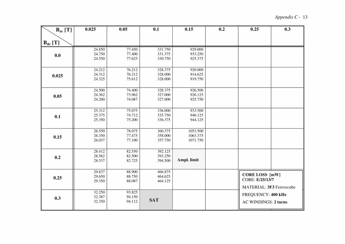
Appendix C - 13
Bac [T] Bdc [T]
0.025 0.05 0.1 0.15 0.2 0.25 0.3
0.0 24.850
24.750
24.550
77.450
77.400
77.625
331.750
331.375
330.750
929.000
933.250
925.375
0.025 24.212
24.312
24.325
76.212
76.212
75.612
328.375
328.000
328.000
920.000
914.625
919.750
0.05 24.500
24.362
24.200
74.400
73.962
74.087
328.375
327.000
327.000
926.500
926.125
925.750
0.1 25.312
25.375
25.350
75.075
74.712
75.200
336.000
335.750
336.375
933.500
946.125
944.125
0.15 26.550
26.350
26.037
78.075
77.475
77.100
360.375
358.000
357.750
1053.500
1063.375
1071.750
0.2 28.412
28.562
28.537
82.550
82.500
82.725
392.125
393.250
394.500
0.25 29.837
29.650
29.350
88.900
88.750
88.087
466.875
464.625
464.125
0.3 32.250
32.387
32.350
93.825
94.150
94.112
CORE LOSS [mW] CORE: E/25/13/7
MATERIAL: 3F3 Ferroxcube
FREQUENCY: 400 kHz
AC WINDINGS: 2 turns
Ampl. limit
SAT
Appendix C - 14
AVERAGE RESULTS
UNITS: Core Losses in mW Magnetic Induction in T
Bac
Bdc
0.025 0.05 0.1 0.15 0.2 0.25 0.3
0.0 1.317 6.890 35.900 100.333 204.200 343.000 523.333
0.025 1.205 6.700 36.100 99.850 204.000 343.000 522.500
0.05 1.215 6.595 36.650 101.000 205.400 339.367 518.000
0.1 1.337 7.830 41.900 108.133 216.750 346.833
0.15 1.630 10.020 52.200 121.300 226.500
0.2 2.535 13.740 66.300 130.725
0.25 3.840 19.797 80.250
0.3 7.170 29.815
Bac
Bdc
0.025 0.05 0.1 0.15 0.2 0.25 0.3
0.0 2.165 14.440 77.625 228.625 475.973 825.120 1276.310
0.025 2.015 14.275 76.820 227.550 472.790 821.685 1271.935
0.05 1.990 14.470 78.295 228.120 475.310 820.620 1266.185
0.1 2.200 16.760 89.065 246.560 498.995 842.122 1276.703
0.15 2.480 20.895 108.730 279.245 533.935 868.810
0.2 3.735 26.945 132.500 314.250
0.25 6.000 36.100 159.685
0.3 10.150 47.155
Bac
Bdc
0.025 0.05 0.1 0.15 0.2 0.25 0.3
0.0 5.717 36.565 221.203 609.122 1287.957 2238.290 3464.583
0.025 5.610 36.170 219.917 606.707 1287.830 2230.220
0.05 5.583 36.357 222.080 612.040 1289.747 2233.540
0.1 5.890 41.287 248.457 659.123 1342.000 2268.663
0.15 7.513 52.413 285.453 738.623 1416.747 2310.625
0.2 9.667 68.213 347.703 817.790 1474.300
0.25 15.647 94.220 411.703 894.203
0.3 28.010 102.393 486.163
CORE: E25/13/7 MATERIAL: 3C85 FREQUENCY: 25 kHz
CORE: E25/13/7 MATERIAL: 3C85 FREQUENCY: 50 kHz
CORE: E25/13/7 MATERIAL: 3C85 FREQUENCY: 100 kHz
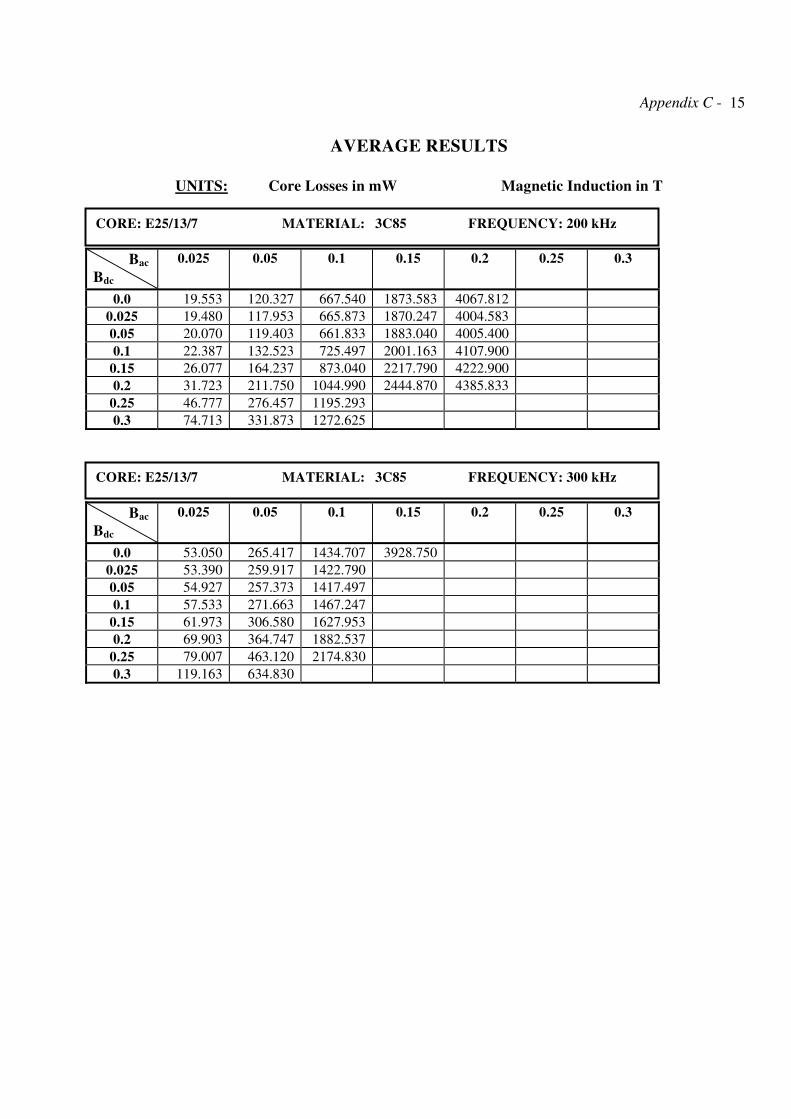
Appendix C - 15
AVERAGE RESULTS
UNITS: Core Losses in mW Magnetic Induction in T
Bac
Bdc
0.025 0.05 0.1 0.15 0.2 0.25 0.3
0.0 19.553 120.327 667.540 1873.583 4067.812
0.025 19.480 117.953 665.873 1870.247 4004.583
0.05 20.070 119.403 661.833 1883.040 4005.400
0.1 22.387 132.523 725.497 2001.163 4107.900
0.15 26.077 164.237 873.040 2217.790 4222.900
0.2 31.723 211.750 1044.990 2444.870 4385.833
0.25 46.777 276.457 1195.293
0.3 74.713 331.873 1272.625
Bac
Bdc
0.025 0.05 0.1 0.15 0.2 0.25 0.3
0.0 53.050 265.417 1434.707 3928.750
0.025 53.390 259.917 1422.790
0.05 54.927 257.373 1417.497
0.1 57.533 271.663 1467.247
0.15 61.973 306.580 1627.953
0.2 69.903 364.747 1882.537
0.25 79.007 463.120 2174.830
0.3 119.163 634.830
CORE: E25/13/7 MATERIAL: 3C85 FREQUENCY: 200 kHz
CORE: E25/13/7 MATERIAL: 3C85 FREQUENCY: 300 kHz
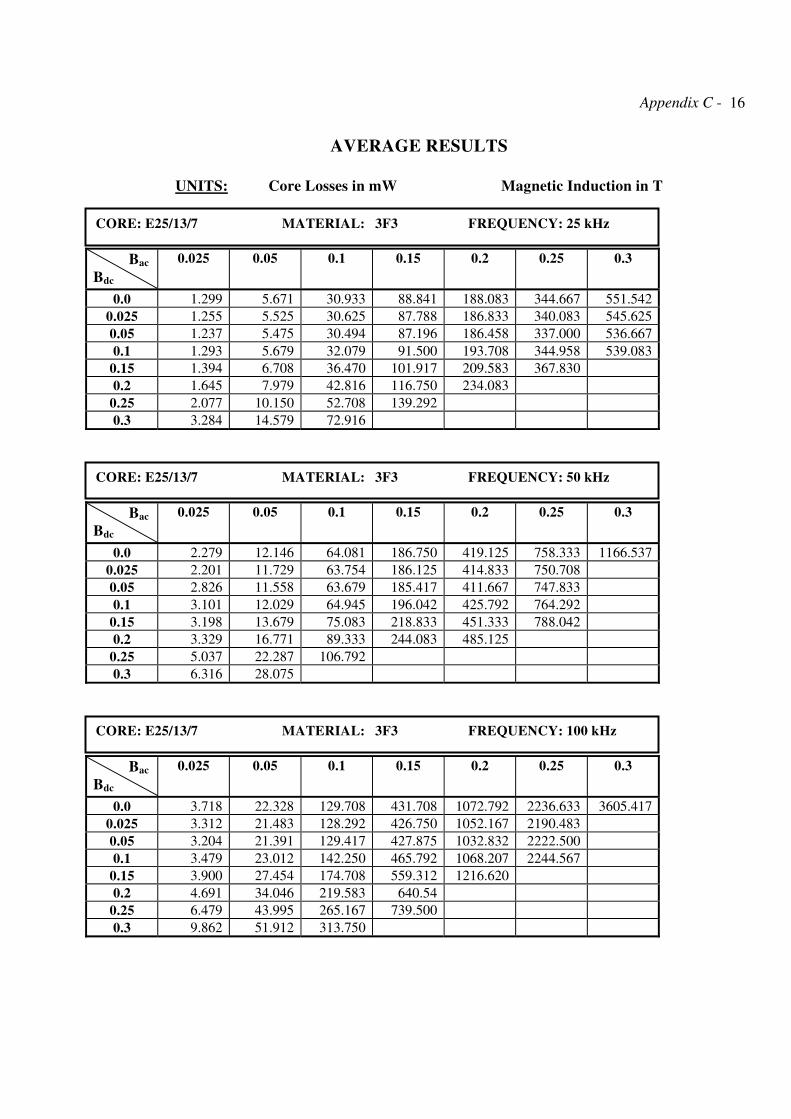
Appendix C - 16
AVERAGE RESULTS
UNITS: Core Losses in mW Magnetic Induction in T
Bac
Bdc
0.025 0.05 0.1 0.15 0.2 0.25 0.3
0.0 1.299 5.671 30.933 88.841 188.083 344.667 551.542
0.025 1.255 5.525 30.625 87.788 186.833 340.083 545.625
0.05 1.237 5.475 30.494 87.196 186.458 337.000 536.667
0.1 1.293 5.679 32.079 91.500 193.708 344.958 539.083
0.15 1.394 6.708 36.470 101.917 209.583 367.830
0.2 1.645 7.979 42.816 116.750 234.083
0.25 2.077 10.150 52.708 139.292
0.3 3.284 14.579 72.916
Bac
Bdc
0.025 0.05 0.1 0.15 0.2 0.25 0.3
0.0 2.279 12.146 64.081 186.750 419.125 758.333 1166.537
0.025 2.201 11.729 63.754 186.125 414.833 750.708
0.05 2.826 11.558 63.679 185.417 411.667 747.833
0.1 3.101 12.029 64.945 196.042 425.792 764.292
0.15 3.198 13.679 75.083 218.833 451.333 788.042
0.2 3.329 16.771 89.333 244.083 485.125
0.25 5.037 22.287 106.792
0.3 6.316 28.075
Bac
Bdc
0.025 0.05 0.1 0.15 0.2 0.25 0.3
0.0 3.718 22.328 129.708 431.708 1072.792 2236.633 3605.417
0.025 3.312 21.483 128.292 426.750 1052.167 2190.483
0.05 3.204 21.391 129.417 427.875 1032.832 2222.500
0.1 3.479 23.012 142.250 465.792 1068.207 2244.567
0.15 3.900 27.454 174.708 559.312 1216.620
0.2 4.691 34.046 219.583 640.54
0.25 6.479 43.995 265.167 739.500
0.3 9.862 51.912 313.750
CORE: E25/13/7 MATERIAL: 3F3 FREQUENCY: 25 kHz
CORE: E25/13/7 MATERIAL: 3F3 FREQUENCY: 50 kHz
CORE: E25/13/7 MATERIAL: 3F3 FREQUENCY: 100 kHz
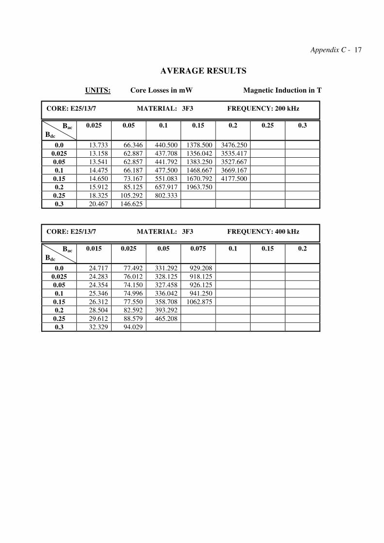
Appendix C - 17
AVERAGE RESULTS
UNITS: Core Losses in mW Magnetic Induction in T
Bac
Bdc
0.025 0.05 0.1 0.15 0.2 0.25 0.3
0.0 13.733 66.346 440.500 1378.500 3476.250
0.025 13.158 62.887 437.708 1356.042 3535.417
0.05 13.541 62.857 441.792 1383.250 3527.667
0.1 14.475 66.187 477.500 1468.667 3669.167
0.15 14.650 73.167 551.083 1670.792 4177.500
0.2 15.912 85.125 657.917 1963.750
0.25 18.325 105.292 802.333
0.3 20.467 146.625
Bac
Bdc
0.015 0.025 0.05 0.075 0.1 0.15 0.2
0.0 24.717 77.492 331.292 929.208
0.025 24.283 76.012 328.125 918.125
0.05 24.354 74.150 327.458 926.125
0.1 25.346 74.996 336.042 941.250
0.15 26.312 77.550 358.708 1062.875
0.2 28.504 82.592 393.292
0.25 29.612 88.579 465.208
0.3 32.329 94.029
CORE: E25/13/7 MATERIAL: 3F3 FREQUENCY: 200 kHz
CORE: E25/13/7 MATERIAL: 3F3 FREQUENCY: 400 kHz
Extended Steinmetz Equation - Bibliography - IV - 1
BIBLIOGRAPHY
1. E. Della Torre, “Magnetic Hysteresis”, IEEE Press and J. Wiley, 1999.
2. G. Bertotti, “Hysteresis in Magnetism”, Academic Press, 1998.
3. E. C. Snelling, “Soft Ferrites: Properties and Applications”, Butterworths, U.K.,1988.
4. R. F. Soohoo, “Theory and Applications of Ferrites”, Prentice-Hall, 1960.
5. S. Smith, “Magnetic Components: Design and Applications”, Van Nostrand Reinhold, 1985.
6. A. Goldman, “Magnetic Components for Power Electronics”, Kluwer Academic Publ., 2002.
7. R. Boll (editor), “Soft magnetics materials: fundamentals, alloys, properties, products and applications”,
Heyden, U.K., 1978.
8. C. W. McLyman, “Magnetic Core Selection for Transformers and Inductors”, M. Dekker, 1997.
9. W. M. Flanagan, “Handbook of Transformer Design and Applications”, McGraw-Hill, 1992.
10. R. M. Bozorth, “Ferromagnetism”, IEEE Press, 1994.
11. M.I.T., E.Eng. Staff, “Magnetic Circuits and Transformers”, The MIT Press, 1951.
12. F. W. Grover, “Inductance Calculations: Working Formulas and Tables”, D. Van Nostrand, 1946.
13. L. Umanand and S. R. Bhat, “Design of Magnetic Components for Switched Mode Power Converters”,
New Age International Ltd. Publ., India, 1992.
14. Philips, “Ferroxcube: Soft Ferrites and Accessories”, Data Book, June 2000, www.ferroxcube.com.
15. Epcos, “Ferrites and Accessories”, Data Book, August 2001, www.epcos.com.
16. D.Y. Chen, “Comparison of high frequency magnetic core losses under two different driving conditions: A
sinusoidal voltage and a square-wave voltage”, IEEE PESC Record , 1978.
17. F. D. Tan, J. L. Vollin and S. M. Cuk, “A practical approach for magnetic core-loss
characterization”, IEEE Trans. on Power Electronics, vol. 10 , No. 2 , 3/1995.
18. W. Roshen, “Ferrite Core Loss for Power Magnetic Components Design”, IEEE Trans. on Magnetics , vol.
27, no. 6, Nov. 1991.
19. J. Li, T. Abdallah, and C. R. Sullivan, “Improved Calculation of Core Loss with Nonsinusoidal
Waveforms”, IEEE Industry Applications Society Annual Meeting, Oct. 2001, Chicago.
20. K. Venkatachalam, C. R. Sullivan, T. Abdallah, and H. Tacca, “Accurate Prediction of Ferrite Core Loss
with Nonsinusoidal Waveforms using Only Steinmetz Parameters”, COMPEL 2002, Jun. 2002, Puerto
Rico.
21. H.E. Tacca, “Flyback vs. Forward Converter Topology Comparison Based upon Magnetic Design”,
Eletrônica de Potência , Vol. 5, no. 1, May 2000, Brazil.
22. J.Reinert, A. Brockmeyer, and R.W. A. A. De Doncker, “Calculation of Losses in Ferro- and Ferrimagnetic
Materials Based on the Modified Steinmetz Equation”, IEEE Transactions on Industry Applications, vol.
37, no. 4, Jul./Aug. 2001.
23. A. Brockmeyer, “Dimensionerungswerkzeug für magnetische Bauelemente in
Stromritchteranwendungen”, Ph.D. dissertation, Inst. Power Electron., Aachen, Germany, 1997.
24. A. Brockmeyer, “Experimental evaluation of the influence of dc-premagnetization on the
properties of power electronic ferrites”, Applied Power Electronics Conference and Exposition
1996 (APEC’96), Vol. 1, 1996.
Extended Steinmetz Equation - Bibliography - IV - 2
25. R. Ridley and A. Nace, “Modeling ferrite core losses”, Switching Power Magazine , January 2002.
26. M. Amar and R. Kaczmarek, “A general formula for prediction of iron losses under nonsinusoidal
voltage waveforms”, IEEE Trans. on Magnetics, vol. 31 , No. 5 , Sept.1995.
27. V. Vorpérian, “Using fractals to model eddy-current losses in ferromagnetic materials”, Switching
Power Magazine , January 2002.
28. W. K. Mo, D. K. W. Cheng, and Y. S. Lee, “Simple Approximations of the DC Flux Influence on the Core
Loss Power Electronic Ferrites and Their Use in Design of Magnetic Components”, IEEE Transactions on
Industrial Electronics, vol.44, no. 6, Dec. 1997.
29. E. Cardelli, L. Fiorucci, and E. Della Torre, “Estimation of MnZn ferrite core losses in magnetic
components at high frequency”, IEEE Trans. on Magnetics, Vol. 37, No. 4, July 2001.
30. A. Balakrishnan, W. T. Joines, and T. G. Wilson, “Air-gap reluctance and inductance calculations for
magnetic circuits using a Schwarz-Christoffel transformation”, IEEE Trans. on Power Electronics , Vol. 12,
No. 4, July 1997.
31. J. Buck, “Automatic hysteresisgraph speeds accurate analysis of soft magnetic materials”, PCIM, February
2000.
32. J. A. Ferreira and J. D. van Wyk, “Experimental evaluation of losses in magnetic components for power
converters”, IEEE Trans. on Industry Applications, Vol. 27, No. 2, March/April 1991.
33. S.-C Wang and C.-L. Chen, “PC-based apparatus for characterizing high frequency magnetic cores”, IEE
Proc. - Sci. Meas. Technology , Vol. 146, no. 6, U.K., Nov. 1999.
34. Iwatsu, “SY-8232 B-H analyzer data sheet”, www.iwatsu.co.jp/tme/pdf/english/sy-8232_e.pdf .
35. R. Linkous, A. W. Kelley, and K. C. Armstrong, “An improved calorimeter for measuring the core loss of
magnetic materials”, IEEE Applied Power Electronics Conf. and Expo. 2000 (IEEE - APEC 2000).
36. V. Leonavicius, M. Duffy, C.O. Mathúna, and U. Boeke, “Comparison of different techniques to realise
PFC boost inductor”, IEEE Applied Power Electronics Conference and Exposition 2002 (IEEE-APEC
2002), Vol. 2, 2002.
37. C. Larouci, J. P. Ferrieux, L. Gerbaud, J. Roudet, and S. Catellani, “Experimental evaluation of the core
losses in the magnetic components used in PFC converters. Application to optimize the flyback structure
losses”, IEEE Applied Power Electronics Conference and Exposition 2002 (IEEE-APEC 2002), Vol. 2,
2002.
38. J. Liu, T. G. Wilson Jr., R. C. Wong, R. Wunderlich, and F. C. Lee, “A method for inductor core loss
estimation in power factor correction applications”, IEEE Applied Power Electronics Conference and
Exposition 2002 (IEEE-APEC 2002), Vol. 2, 2002.
39. G. D’Antona et al., “AC measurements via digital processing of Rogowski coils signal”, IEEE
Instrumentation and Measurement Technology Conference , Anchorage, USA, May 2002.
40. W. F. Ray and C. R. Hewson, “High performance Rogowski current transducers”, IEEE Industry
Applications Conference , 2000.
41. W. F. Ray, “Rogowski transducers for high bandwidth high current measurement”, IEE Colloquium on Low
Frequency Power Measurement and Analysis (Digest No. 1994/203), U.K., 1994.
42. W. F. Ray, “The use of Rogowski coils for low amplitude current waveform measurement”, IEE
Colloquium on Measurement Techniques for Power Electronics, U.K., 1992.
43. C. Alarcón, A. Godel, M. Pupareli, “Proyecto de inductores con circulación de C.A. y C.C. superpuestas”,
Rev. Telegráfica Electrónica, Buenos Aires, 11/1977.