Embed Size (px)
Citation preview

Extensions of Poisson Geometric ProcessModel with Applications
WAI-YIN WAN
A thesis submitted in fulfillment ofthe requirements for the degree of
Doctor of Philosophy
School of Mathematics and StatisticsThe University of Sydney
August 2010

Abstract
The modelling of longitudinal and panel count data has a rich history.
Despite the well-established time series count models, we seek a new direc-
tion to study panel and multivariate longitudinal count data with different
characteristics.
We extend the Poisson geometric process (PGP) model introduced by
Wan (2006) in the modelling of non-monotone trend for time series of
counts. The PGP model is developed from the geometric process (GP)
model pioneered by Lam (1988a) and Lam (1988b) to study positive con-
tinuous data with monotone trend. Lam (1988a) and Lam (1988b) states
that a stochastic process (SP) {Xt, t = 1, 2, . . . } is a GP if there exists a
positive real number a > 0 such that {Yt = at−1Xt} generates a renewal
process (RP) with mean E(Yt) = µ and variance V ar(Yt) = σ2 where a is
the ratio of the GP.
Under the GP framework, the PGP model assumes that the countWt, t =
1, . . . , n follows a Poisson distribution with meanXt where {Xt, t = 1, . . . , n}forms a latent GP and the corresponding SP {Yt} follows some lifetime dis-
tributions with E(Yt) = µt and V ar(Yt) = σ2t . The PGP model focuses
on the modelling of the latent stationary SP instead of the latent GP and
separates the effects on trend movement from the effects on the underly-
ing system (SP) that generates the GP by individually modelling the ratio
and the mean of the SP. This merit of the model enhances its applicability
i
ABSTRACT ii
in analyzing longitudinal and panel count data with non-monotone trends,
overdispersion and cluster effects.
In view of other prominent characteristics including presence of excess
zeros or outliers, diverse degrees of dispersion and serial correlation be-
tween observations, we extend the PGP model to take into account all these
problems in turn by adopting different distributions for {Yt}, replacing the
Poisson data distribution with generalized Poisson distribution with more
flexible dispersion structure and incorporating some past observations as
time-evolving covariates in the mean link function. Moreover, concern-
ing the lack of literature in the modelling of multivariate longitudinal count
data, we consider a multivariate version of the PGP model to cope with con-
temporaneous correlation and cross correlation between time series on top
of the other characteristics.
For statistical inference, these extended models are implemented using
Markov chain Monte Carlo (MCMC) algorithms to avoid the evaluation of
complicated likelihood functions and their derivatives which may involve
high-dimensional integration. To demonstrate the properties and applica-
bilities of these models, a series of simulation studies and real data analyses
are conducted. All in all, the extended PGP models taken into account all
the pronounced characteristics of time series of counts are shown to provide
satisfactory performance in both simulation studies and real data analyses.
They certainly can become competitive alternatives to the traditional time
series count models in the future.

Declaration
I declare that this thesis represents my own work, except where due
acknowledgement is made, and that it has not been previously included in
a thesis, dissertation or report submitted to this University or to any other
institution for a degree, diploma or other qualifications.
Signed
Wai Yin WAN
iii

Acknowledgements
First and foremost, I owe my deepest and sincere gratitude to my pri-
mary supervisor, Dr. Jennifer S. K. Chan, at the School of Mathematics and
Statistics, The University of Sydney. Her rich intellect, inspiration, enor-
mous guidance and intimate encouragement have provided a good basis for
the present thesis. She has been a role model in her diligence in research,
enthusiasm in teaching and ingenuity of ideas, to a mediocre student who
left her family to go abroad and sometimes loses the direction in midst of
difficulties. Secondly, I would also like to thank my associate supervisor,
Dr. Boris Choy who has perpetual energy and enthusiasm in research. His
insights and innovative ideas motivate me and broadens my perspective on
future career development. Moreover, it is a pleasure to thank Prof. Neville
Weber, my second associate supervisor, who offers me the opportunity to
start my research degree in this renowned University and all the friends and
staff in the School for their cares and support. Without any of them, I would
not have such wonderful experiences.
Above all, I am indebted to my family and boyfriend for always sup-
porting me unceasingly and encouraging me to move on and I would also
like to thank God to equip me with the mathematical ability to study sta-
tistics. Their endless love and support have been invaluable in helping me
to focus on my academic pursuits. Without them, I would not have had the
courage to complete this thesis.
iv

CONTENTS
Abstract . . . . . . . . . . . . . . . . . . . . . . . . . . . . . . . . . . . . . . . . . . . . . . . . . . . . . . . . i
Declaration . . . . . . . . . . . . . . . . . . . . . . . . . . . . . . . . . . . . . . . . . . . . . . . . . . . . . iii
Acknowledgements . . . . . . . . . . . . . . . . . . . . . . . . . . . . . . . . . . . . . . . . . . . . . iv
List of Figures . . . . . . . . . . . . . . . . . . . . . . . . . . . . . . . . . . . . . . . . . . . . . . . . . . vii
List of Tables . . . . . . . . . . . . . . . . . . . . . . . . . . . . . . . . . . . . . . . . . . . . . . . . . . . ix
Chapter 1. Introduction . . . . . . . . . . . . . . . . . . . . . . . . . . . . . . . . . . . . . . . 1
1.1. Background . . . . . . . . . . . . . . . . . . . . . . . . . . . . . . . . . . . . . . . . . . . . . 1
1.2. Overview of longitudinal count models . . . . . . . . . . . . . . . . . . . . 4
1.3. Overview of geometric process models . . . . . . . . . . . . . . . . . . . . . 11
1.4. Statistical inference . . . . . . . . . . . . . . . . . . . . . . . . . . . . . . . . . . . . . . 22
1.5. Objective and structure of thesis . . . . . . . . . . . . . . . . . . . . . . . . . . . 30
Chapter 2. Mixture Poisson geometric process model . . . . . . . . . . . 34
2.1. Background . . . . . . . . . . . . . . . . . . . . . . . . . . . . . . . . . . . . . . . . . . . . . 34
2.2. Bladder cancer data . . . . . . . . . . . . . . . . . . . . . . . . . . . . . . . . . . . . . . 37
2.3. MPGP model and its extension . . . . . . . . . . . . . . . . . . . . . . . . . . . . 38
2.4. Bayesian Inference . . . . . . . . . . . . . . . . . . . . . . . . . . . . . . . . . . . . . . . 44
2.5. Real data analysis . . . . . . . . . . . . . . . . . . . . . . . . . . . . . . . . . . . . . . . . 51
2.6. Discussion . . . . . . . . . . . . . . . . . . . . . . . . . . . . . . . . . . . . . . . . . . . . . . 58
Chapter 3. Robust Poisson geometric process model . . . . . . . . . . . . 68
3.1. Background . . . . . . . . . . . . . . . . . . . . . . . . . . . . . . . . . . . . . . . . . . . . . 68
v

CONTENTS vi
3.2. Model specification . . . . . . . . . . . . . . . . . . . . . . . . . . . . . . . . . . . . . . 74
3.3. Bayesian inference . . . . . . . . . . . . . . . . . . . . . . . . . . . . . . . . . . . . . . . 80
3.4. Simulation study . . . . . . . . . . . . . . . . . . . . . . . . . . . . . . . . . . . . . . . . . 89
3.5. Real data analysis . . . . . . . . . . . . . . . . . . . . . . . . . . . . . . . . . . . . . . . . 91
3.6. Discussion . . . . . . . . . . . . . . . . . . . . . . . . . . . . . . . . . . . . . . . . . . . . . . 100
Chapter 4. Generalized Poisson geometric process model . . . . . . . 115
4.1. Background . . . . . . . . . . . . . . . . . . . . . . . . . . . . . . . . . . . . . . . . . . . . . 115
4.2. Model specification . . . . . . . . . . . . . . . . . . . . . . . . . . . . . . . . . . . . . . 119
4.3. Bayesian inference . . . . . . . . . . . . . . . . . . . . . . . . . . . . . . . . . . . . . . . 126
4.4. Simulation studies . . . . . . . . . . . . . . . . . . . . . . . . . . . . . . . . . . . . . . . 131
4.5. Real data analysis . . . . . . . . . . . . . . . . . . . . . . . . . . . . . . . . . . . . . . . . 138
4.6. Discussion . . . . . . . . . . . . . . . . . . . . . . . . . . . . . . . . . . . . . . . . . . . . . . 149
Chapter 5. Multivariate generalized Poisson log-t geometric
process model . . . . . . . . . . . . . . . . . . . . . . . . . . . . . . . . . . . . . . 160
5.1. Background . . . . . . . . . . . . . . . . . . . . . . . . . . . . . . . . . . . . . . . . . . . . . 160
5.2. A review of multivariate Poisson models . . . . . . . . . . . . . . . . . . . 166
5.3. Multivariate generalized Poisson log-t geometric process
model . . . . . . . . . . . . . . . . . . . . . . . . . . . . . . . . . . . . . . . . . . . . . . . . . . 172
5.4. Bayesian inference . . . . . . . . . . . . . . . . . . . . . . . . . . . . . . . . . . . . . . . 182
5.5. Real data Analysis . . . . . . . . . . . . . . . . . . . . . . . . . . . . . . . . . . . . . . . 187
5.6. Discussion . . . . . . . . . . . . . . . . . . . . . . . . . . . . . . . . . . . . . . . . . . . . . . 199
Chapter 6. Summary . . . . . . . . . . . . . . . . . . . . . . . . . . . . . . . . . . . . . . . . . . 211
6.1. Overview . . . . . . . . . . . . . . . . . . . . . . . . . . . . . . . . . . . . . . . . . . . . . . . 211
6.2. Further research . . . . . . . . . . . . . . . . . . . . . . . . . . . . . . . . . . . . . . . . . 216
Bibliography . . . . . . . . . . . . . . . . . . . . . . . . . . . . . . . . . . . . . . . . . . . . . . . . . . . 219

List of Figures
2.1 Trends of new tumour counts using ZMPGP model (Model 3) . . . . 65
2.2 Trends of new tumour counts using MPGP-Ga model (Model 4) . . . 66
2.3 Proportions of zeros and variances of new tumour counts for Model
1 to 4 . . . . . . . . . . . . . . . . . . . . . . . . . . . . . . . . . . . . . . . . . . . . . . . . . . . . . . . 67
3.1 The pmfs of RPGP-t model with varying parameters . . . . . . . . . . . . . 108
3.2 The pmfs of RPGP-EP model with varying parameters . . . . . . . . . . . 109
3.3 pmf of 2-group RMPGP-EP model at t = 1 . . . . . . . . . . . . . . . . . . . . . 110
3.4 Dotplots of seizure counts across treatment group and time . . . . . . . 111
3.5 The pmfs of low-level group for RMPGP models at different times 112
3.6 Comparison of densities of yitl’s with normal and EP distributions . 113
3.7 Outlier diagnosis using uitl in the RMPGP-EP model . . . . . . . . . . . . 114
4.1 The pmfs of GPGP model with varying parameters . . . . . . . . . . . . . . 156
4.2 Observed and predicted trends of GMPGP and RMPGP-EP models157
4.3 The pmfs of high-level group for GMPGP and RMPGP-EP models
at different t . . . . . . . . . . . . . . . . . . . . . . . . . . . . . . . . . . . . . . . . . . . . . . . . . 158
4.4 The pmfs of low-level group for GMPGP and RMPGP-EP models
at different t . . . . . . . . . . . . . . . . . . . . . . . . . . . . . . . . . . . . . . . . . . . . . . . . . 158
4.5 Predicted individual and group trends of GMPGP-AR(1) model . . . 159
5.1 The pmfs of BGPLTGP model with varying parameters . . . . . . . . . . 206
vii

LIST OF FIGURES viii
5.1 The pmfs of BGPLTGP model with varying parameters (continued)207
5.2 Monthly number of arrests for amphetamine (AMP) and narcotics
(NAR) use/possession in Sydney during January 1995 - December
2008 . . . . . . . . . . . . . . . . . . . . . . . . . . . . . . . . . . . . . . . . . . . . . . . . . . . . . . . . 208
5.3 Trends of the expected monthly number of arrests for use or
possession of two illicit drugs for all fitted models . . . . . . . . . . . . . . . 209
5.4 Trends of the SE of monthly number of arrests for use or
possession of two illicit drugs for all fitted models . . . . . . . . . . . . . . . 210

List of Tables
2.1 Parameter estimates, SE (in italics) and DIC in different PGP
models for the bladder cancer data . . . . . . . . . . . . . . . . . . . . . . . . . . . . . 64
3.1 Moments of marginal pmfs for RPGP-t model under a set of
floating parameters with fixed values of ν = 10, σ = 0.5, βµ0 =
3, βµ1 = −0.2, βa0 = 0.5, βa1 = −0.1 . . . . . . . . . . . . . . . . . . . . . . . . . . 104
3.2 Moments of marginal pmfs for RPGP-EP model under a set of
floating parameters with fixed values of ν = 1, σ = 0.5, βµ0 =
3, βµ1 = −0.5, βa0 = 0.5, βa1 = −0.1 . . . . . . . . . . . . . . . . . . . . . . . . . . 104
3.3 Parameter estimates, SD, MSE, DIC and ASE in different
RPGP models under 4 simulated data sets based on 4 sets of true
parameters from different models . . . . . . . . . . . . . . . . . . . . . . . . . . . . . . 105
3.4 Mean and variance for the observed epilepsy data and of two
simple fitted and RMPGP-EP models . . . . . . . . . . . . . . . . . . . . . . . . . . . 106
3.5 Parameter estimates with SE and DIC in different RMPGP
models for the epilepsy data . . . . . . . . . . . . . . . . . . . . . . . . . . . . . . . . . . . 107
4.1 Moments of marginal pmfs for GPGP model under a set of floating
parameters with fixed values of λ2 = 0.2, r = 30, βµ0 = 3, βµ1 =
−0.5, βa0 = −0.5, βa1 = 0.2 . . . . . . . . . . . . . . . . . . . . . . . . . . . . . . . . . . . 152
4.2 Parameter estimates, SD,MSE andDIC for GPGP and RPGP-EP
models in cross simulation (Study 1) . . . . . . . . . . . . . . . . . . . . . . . . . . . 152
ix

LIST OF TABLES x
4.3 Mean and variance of the true, GPGP and RPGP-EP models in
cross simulation (Study 1) . . . . . . . . . . . . . . . . . . . . . . . . . . . . . . . . . . . . . 153
4.4 Mean and variance of four simulated data sets under different
situations (Study 2) . . . . . . . . . . . . . . . . . . . . . . . . . . . . . . . . . . . . . . . . . . . 153
4.5 Parameter estimates, SE and DIC in GPGP and RPGP-EP models
under different degrees of dispersion (Study 2) . . . . . . . . . . . . . . . . . . 154
4.6 Parameter estimates, SE and DIC in 2-group GMPGP and
RMPGP-EP models for the cannabis data . . . . . . . . . . . . . . . . . . . . . . . 154
4.7 Observed and predicted means and variances of GMPGP and
RMPGP-EP models for the cannabis data . . . . . . . . . . . . . . . . . . . . . . . 155
5.1 Moments of the joint pmfs for the BGPLTGP model under a set
of floating parameters with fixed values of σ21 = 0.07, σ12 =
0.06, σ22 = 0.1, ν = 20, βµ01 = 2, βµ02 = 2.5, βa01 = −0.1, βa02 =
0.1, λ21 = −0.8, λ22 = 0.2 . . . . . . . . . . . . . . . . . . . . . . . . . . . . . . . . . . . . 203
5.2 Parameter estimates, SE and DIC in four fitted models for the
amphetamine and narcotics data . . . . . . . . . . . . . . . . . . . . . . . . . . . . . . . 204
5.3 Parameter estimates, SE and DIC in BGPLTGP model after
accounting for serial correlation. . . . . . . . . . . . . . . . . . . . . . . . . . . . . . . . 205

CHAPTER 1
Introduction
1.1. Background
Analysis of event count data which prevails in all walks of lives has a
long and rich history. In epidemiology, we observe the daily number of
deaths in an epidemic outbreak; in engineering, we record the number of
failures of an operating system until it breaks down; in business, we count
the number of mobile phones sold every week for different phone models
or brands; in insurance, we report the claim frequencies for a compulsory
third party insurance policy. The list of areas in which time series of counts
are observed and analyzed is endless.
Event count can be classified into three main categories including cross-
sectional, longitudinal and panel. Different from cross-sectional data which
is collected from a number of individuals at the same time point, longi-
tudinal data, also known as time series data, are observations repeatedly
measured from one subject over a series of time. If there are multiple out-
comes observed at the same time, the outcomes that are potentially corre-
lated is called multivariate longitudinal data. Regarded as a more general
case, panel data is a set of longitudinal data collected from a number of
1

1.1. BACKGROUND 2
subjects. In this thesis, we will focus on the analysis of multivariate longi-
tudinal count data and panel count data.
Longitudinal or panel count data are frequently obtained in follow-up
or prospective studies such as randomized clinical trials in which the re-
current number of events is usually recorded successively at uniform time
intervals. Inevitably, the non-stationarity and serial correlation structure in
the time series make the modelling of panel data distinct and more compli-
cated than cross-sectional data. In non-stationary time series, an increas-
ing (or decreasing) trend often coincides with an increasing (or decreasing)
variability in the data over time. When the mean is larger (smaller) than
the variance, we refer such situation as underdispersion (or overdispersion).
Ignoring the dispersion problems may lead to poor model fit, unreliable es-
timates and hence misleading interpretations.
Besides, exogenous covariates which can be time-invariant, time-variant
or period-variant, are commonly measured along with the outcomes. For
instance, in a tobacco use study, the weekly number of cigarettes taken by
smokers may be affected by sex and age to start smoking which are time-
invariant, number of doctor visits and alcohol consumption which are time-
variant, and lastly income and education level which are period-variant. In-
cluding these covariates into the mean of the data distribution helps to in-
vestigate their effects on the outcome or allow for their effects in the studies
of other variables of interest. For example, in a randomized clinical trial

1.1. BACKGROUND 3
on the efficacy of a medication for hypertension, undoubtedly the differ-
ence between the control group and treatment group is of primary interest.
Moreever, sex, age or other measures of health condition which may affect
the treatment result are regarded as nuisance variables and should also be
allowed for in the study of treatment effect.
Particularly for panel count data which involves multiple subjects with
different characteristics, population heterogeneity will arise inevitably. Tak-
ing the previous example of the hypertension medication study, between-
subject variation may exist across each group of patients as the treatment
may work better on some patients or due to measurement errors. In the
past decades, extensive literature can be found in analyzing longitudinal and
panel data. In these researches, extensions have been made continuously to
some existing traditional count models to address all the aforementioned
properties in the data.
This thesis focuses on the development of models for longitudinal or
panel count data that can handle various characteristics of the count data
arisen in different situations. The following section will first summarize
briefly a few benchmarking models for modelling longitudinal count data
and how they are developed and modified to study multivariate longitudinal
and panel count data. The next two Sections will describe the development
and method of inference of geometric process (GP) model from which the
Poisson geometric process (PGP) model is developed and is adopted as the

1.2. OVERVIEW OF LONGITUDINAL COUNT MODELS 4
start-up model in this research due to its indispensable ability to allow trend
movement.
1.2. Overview of longitudinal count models
Based on the theory of state-space models, Cox (1981) classified the
longitudinal count models into two streams, namely the observation-driven
(OD) and parameter-driven (PD) models. A good monograph on the clas-
sification can be found in Cameron & Trivedi (1998). Denote Wt be the
outcome at time t = 1, . . . , n where n is the total number of observations.
The state-space model consists of an observation equation which specifies
the distribution of the outcome Wt given the state variable and a state equa-
tion which specifies the transition distribution of the state variable. For both
OD and PD models, while the observation equations are tantamount as they
assume Wt follows some discrete distributions f(wt) such as Poisson and
negative binomial distributions given the mean E(Wt) as the state variable,
their difference lies in the specification of the state equation for E(Wt).
The OD models express the mean of the outcome explicitly as a function
of past observations in order to construct an autocorrelation structure which
can account for serial correlation between observations. On the other hand,
the PD models introduce serial dependence through a latent variable which
evolves independently of the past observations in the state equation. In the
following Sections, a few benchmarking OD and PD models with model
structures and extensions to multivariate longitudinal or panel count data
will be discussed.
1.2. OVERVIEW OF LONGITUDINAL COUNT MODELS 5
1.2.1. Observation-driven models. The OD models are so called be-
cause they introduce past observations into the mean of the current observa-
tion. An important class of the OD models is the integer-valued autoregres-
sive moving average (INARMA) model developed under the framework of
Gaussian autoregressive moving average (ARMA) model. This model pio-
neered by Al-Osh & Alzaid (1987) has developed extensively and a recent
survey can be found in McKenzie (2003).
Under the INARMA model the outcome Wt is expressed as
Wt =
p∑
i=1
αi ◦Wt−i +
q∑
j=1
γj ◦ Ut−j + Ut
where Ut, t = 1, . . . , n are non-negative latent integer-valued variables that
are independently and identically distributed and ◦ is a binomial thinning
operator such that
αi◦Wt−i =
Bin(Wt−i, αi), Wt−i > 0
0, Wt−i = 0and γj◦Ut−j =
Bin(Ut−j, γj), Ut−j > 0
0, Ut−j = 0
In other words, αi, γj ∈ [0, 1] denote the probability of success for the bi-
nomial distribution for Wt−i and Ut−j respectively. Let xt and β be vectors
of time-evolving covariates and regression coefficients respectively, then
the mean of Ut can be log-linked to a function of covariates xt so that
E(Ut) = exp(xTt β). The resultant model is denoted as INARMA(p, q)
model where p represents the autoregressive (AR) order for the observa-
tions and q specifies the moving average (MA) order for the errors.
1.2. OVERVIEW OF LONGITUDINAL COUNT MODELS 6
Taking INARMA(1,0) model as an example, the conditional mean and
variance for Wt are given by
E(Wt|Wt−1, . . . ) = α1Wt−1 + exp(xTt β)
V ar(Wt|Wt−1, . . . ) = α1(1 − α1)Wt−1 + V ar(Ut)
and the autocorrelation function Corr(Wt,Wt−k) = αk1 is always positive.
So, this model is restricted to positively serially correlated data.
A multivariate extension of the INARMA model can be found in Quore-
shi (2008). Denote the data vector W t = {Wit, ...,Wmt}T with dimension
m, the extended model called the vector integer-valued moving average
(VINMA) model has the following form:
W t =
q∑
j=1
γj ◦ U t−j + U t
W1t
W2t
...
Wmt
=
q∑
j=1
γ11q γ12q . . . γ1mq
γ21q γ22q . . . γ2mq
... . . .. . .
...
γm1q γm2q . . . γmmq
◦
U1,t−q
U2,t−q
...
Um,t−q
+
U1t
U2t
...
Umt
where U t = {U1t, ..., Umt}T is an integer-valued innovation sequence which
is independently and identically distributed with its mean log-linked to some
time-variant covariates xit such that E(Uit) = exp(xTitβi), i = 1, . . . ,m
where βi is vector of regression coefficients for Wit. Besides accommodat-
ing covariate effects, the VINMA model is capable of fitting multivariate
longitudinal count data with both negative or positive correlation between

1.2. OVERVIEW OF LONGITUDINAL COUNT MODELS 7
pairs of time series. See Quoreshi (2008) for more details. However, Heinen
(2003) criticized that the INARMA model is not practically applicable due
to its cumbersome estimation of the model parameters. Hence emphases
were only put on the studies of their stochastic properties.
To tackle the estimation problem, Davis et al. (1999) and Davis et al.
(2003) proposed the generalized linear autoregressive moving average (GLARMA)
model where Wt given the past history Ft−1 follows Poisson distribution
with mean µt and is denoted by
Wt|Ft−1 ∼ Poi(µt)
and µt = exp(xTt β + Ut). Furthermore,
Ut = φ1Ut−1 + · · · + φp Ut−p +
q∑
i=1
θiet−i
where Ut is an ARMA(p, q) process with noise
{et =
Wt − µt
µλt
}, λ ∈
(0, 1] and past errors et−i which describe the correlation structure of Wt.
The GLARMA model can allow for serial correlation in the count data by
specifying the log of the conditional mean process as a linear function of
previous counts. The main advantage of the GLARMA model is the effi-
cient model estimation using maximum likelihood (ML) method in contrast
to the INARMA model. This greatly widens the applications of the model
to time series of counts.
Another benchmarking OD model is the autoregressive conditional Pois-
son (ACP) model emerged in Heinen (2003). Given the past observations

1.2. OVERVIEW OF LONGITUDINAL COUNT MODELS 8
Ft−1, the outcome Wt follows a Poisson distribution with mean µt which is
written as
E(Wt|Ft−1) = µt = (ω +
p∑
i=1
αiWt−i +
q∑
j=1
γjµt−j) exp(xTt β)
where ω, αi’s and γj’s > 0 and again xt and β are vectors of time-variant
covariates and regression coefficients. Hence, the resultant model, which
is denoted by ACP(p, q) model, has an autoregressive structure introduced
by a recursion on lagged observations. In the same paper, he further ex-
tended the ACP model by replacing the Poisson distribution with Dou-
ble Poisson distribution which can fit underdispersed or overdispersed data
and by adding a generalized autoregressive conditional heteroskedasticity
(GARCH) component to allow a time-varying variance structure. The re-
sulting generalized conditional autoregressive Double Poisson (GDACP)
model can deal with data with underdispersion or overdispersion and posi-
tive serial correlation.
A multivariate extension of the GDACP (MDACP) model has recently
been investigated by Heinen & Rengifo (2007) using copulas to introduce
dependence among several time series. This MDACP model, having similar
properties as the GDACP model, can also accommodate positive or nega-
tive correlation among time series. See Heinen & Rengifo (2007) for more
details.
In summary, the appeals of the OD models include the straightforward
derivation of likelihood function and prediction. On the other hand, being
a conditional rather than marginal model over past observations, they have
1.2. OVERVIEW OF LONGITUDINAL COUNT MODELS 9
a shortcoming in the interpretation of covariate effects as the mean depends
on past observations. In the light of this, another class of count models, the
PD models were proposed to alleviate these problems.
1.2.2. Parameter-driven models. The most prominent PD model in
the literature is the Poisson regression model with stochastic autoregres-
sive mean developed by Zeger (1988). This model is essentially a log lin-
ear model in the family of generalized linear model (GLM) formulated by
Nelder & Wedderburn (1972). Conditional on a latent non-negative stochas-
tic process {Ut} and a vector of time-variant covariates xt, assume that the
outcome Wt is independent and follows a Poisson distribution with mean
µt, then the conditional mean and variance are specified as
E(Wt|Ut) = V ar(Wt|Ut) = µtUt = exp(xTt β)Ut
where β is a vector of regression coefficients. To introduce both serial
correlation and extra variation to the model, suppose that the latent process
Ut is stationary and serially correlated with mean E(Ut) = 1, variance
V ar(Ut) = σ2u and covariance Cov(Ut, Ut−k) = σ2
uρk where ρk represents
the correlation between Ut and Ut−k. The unconditional moments are then
given by
E(Wt) = exp(xTt β)
V ar(Wt) = µt + σ2uµ
2t
Cov(Wt,Wt−k) = µt µt−k σ2u ρk.
1.2. OVERVIEW OF LONGITUDINAL COUNT MODELS 10
Clearly the model is suitable for longitudinal count data with overdispersion
since the variance is larger than the mean and allows both positive or nega-
tive serial correlation as −1 ≤ ρk ≤ 1. More importantly, the time-varying
variance and covariance increase the flexibility of the model structure in
fitting data with non-constant variance and serial correlation. Some appli-
cations of this model can be found in Chan & Ledolter (1995) and Jung &
Liesenfeld (2001) by adopting a Gaussian first order autoregressive struc-
ture for Ut.
Noticing the increasing need of modelling panel count data in a variety
of areas, Zeger et al. (1988) extended the aforementioned GLM to a gen-
eralized linear mixed model (GLMM) by adding random effects to account
for subject-specific effects in the panel data. Assume Wit be the outcome
of subject i, i = 1, . . . ,m at time t, t = 1, . . . , n, xit and zit be vectors
of subject-specific time-variant covariates and U = {U T1 , . . . ,U
Tm}T be
a qm × 1 vector of random effects. Under the GLMM, the outcome Wit
follows a Poisson distribution with mean µit which can be expressed as
µit = exp(xTitβ + zT
itU i)
where U i is assumed to be a multivariate normal variable. Later Brannas &
Johansson (1996) relaxed the independent assumption such thatCov(U i,U j) 6=
0 in order to allow for correlation between different pairs of time series.
Nevertheless, enormous literature emerged afterwards to modify the model
structure such as allowing correlation between covariates and random ef-
fects (Windmeijer, 2000) and replacing the underlying Poisson distribution

1.3. OVERVIEW OF GEOMETRIC PROCESS MODELS 11
with other discrete distributions. See Winkelmann (2008) for a up-to-date
survey of statistical techniques for the analysis of count data.
In contrast to the OD models, the specification of a latent stochastic
process in the PD models enables a straightforward interpretation of the co-
variate effects on the outcome because they are formulated independent of
the past observations. Yet in general, there exists difficulties in forecasting
since the model is built on a latent process and the estimation of parameters
requires considerable computational effort as the likelihood function con-
taining multiple integrals is difficult to evaluate (Jung & Liesenfeld, 2001).
1.3. Overview of geometric process models
Overall, the OD and PD models focus on modelling overdispersion
and serial correlation in longitudinal and panel count data while leaving
the trend of the time series unattended. Evaluating the trend movement
is important since it provides invaluable information for ‘long-term’ pol-
icy assessment, evaluation, planning and development in many studies of
longitudinal count data, for example, in public health where clinical trials
are conducted to study the efficacy of a treatment with respect to the long-
term improvements of certain health variables, or in socioeconomics where
policies are made based on the consistent and prolonged change of certain
economic indicators.
This research extends the Poisson geometric process (PGP) model in
Wan (2006) to allow for various characteristics of longitudinal and panel
count data especially the trend movements. The PGP model is developed

1.3. OVERVIEW OF GEOMETRIC PROCESS MODELS 12
from the GP model proposed by Lam (1988a) and Lam (1988b) for mono-
tone positive continuous data. This GP model offers a straightforward ap-
proach to extend the PGP model for analyzing longitudinal and panel count
data with monotone as well as non-monotone trend. The next Section will
give a detailed discussion of the development and applications of the GP
models on different types of data.
1.3.1. Geometric process model. In system maintenance, due to ac-
cumulating deterioration, the failure rate of the system increases gradually
resulting in a monotone decreasing trend in the consecutive operating times.
Nonhomogeneous Poisson process has been used for trend data. If the suc-
cessive inter-arrival times are monotone, the Cox-Lewis model and expo-
nential process model are commonly used. Lam (1988a) and Lam (1988b)
on the other hand introduced a more direct approach, the geometric pro-
cess (GP) to analyze the trend in such monotone process. The GP model is
defined as follows.
Definition. Given a sequence of random variables {Xt, t = 1, 2, . . . }, if
for some a > 0, {Yt = at−1Xt} forms a renewal process (RP) (Feller,
1949), then {Xt} is called a geometric process (GP), and the real number a
is called the ratio of the GP.
The GP model asserts that if the ratio a discounts Xt geometrically by
t − 1 times, the resulting process {Yt} becomes stationary and forms a
RP, which may follow some parametric distributions f(yt) such as expo-
nential, gamma, Weibull and lognormal distributions with E(Yt) = µ and
1.3. OVERVIEW OF GEOMETRIC PROCESS MODELS 13
V ar(Yt) = σ2. Hence, the mean and variance of the GP model are:
E(Xt) =µ
at−1and V ar(Xt) =
σ2
a2(t−1)
respectively. Clearly, the GP model allows the mean and variance of the
outcome to change over time so that any non-stationarity and non-constant
volatility in the data can be allowed for. The moments are controlled by
three parameters µ, a, and σ2. The inverse relationship of the ratio a with
the mean E(Xt) explains why the trend becomes monotonically increasing
when a < 1 but decreasing when a > 1. When a = 1, it becomes a
stationary RP which is independently and identically distributed with the
same distribution f(yt).
The merits of the GP model are twofold: its geometric structure and
a ratio parameter a to model non-stationarity. Firstly, the model assumes
that the observed data at time t form a latent RP after discounted by a ratio
parameter a for t− 1 times. Such a geometric structure often exists in sys-
tems that generate time series. The GP model focuses on the modelling of
the latent stationary RP instead of the observed GP. By individually mod-
elling the ratio and the mean of the RP, the model separates the effects
on trend movement from the effects on the underlying system (the latent
RP) that generates the observed GP. This approach is natural and appealing.
Moreover the latent RP forms the state parameter of a state space model
and hence can adjust for model dispersion and achieve model robustness
by suitably assigning some heavy-tailed distributions to the latent RP. Sec-
ondly, the additional ratio parameter a makes the two-component (mean
1.3. OVERVIEW OF GEOMETRIC PROCESS MODELS 14
and ratio) GP model a different but simple modelling approach to capture
various characteristics, particularly the trend movement in time series.
With these nice features and simple model structure, the GP models
have been widely applied in modelling inter-arrival times with monotone
trend for the reliability and maintenance problems in the optimal replace-
ment or repairable models (Lam, 1988a,b, 1992a,b). For example, Lam
(1992b) succeeded in fitting the GP model to the inter-arrival times of the
unscheduled maintenance actions for the U.S.S. Halfbeak No.3 and No. 4
main propulsion diesel engines. Moreover Lam & Zhang (1996a) analyzed
the successive operating times in a two-component system arranged in se-
ries while Lam (1995) and Lam & Zhang (1996b) studied the times in a
two-component system emerged in parallel. More examples can be found
in Lam (1997), Lam et al. (2002), Lam & Zhang (2003), Lam et al. (2004),
Zhang (1999), Zhang et al. (2001), Zhang (2002) and Zhang et al. (2002).
In most cases, the inter arrival times exhibit time-variant or time-invariant
covariate effects, for instances, the operating time of a system is possibly
affected by the environmental factors like humidity and temperature of the
working site. Hence, adopting a homogeneous mean µ will be too restric-
tive in reality. Similar to GLM, the GP model can accommodate covariate
effects by log-linking a linear function of some time-evolving covariates to
the mean µ of the lifetime distribution f(yt) such that µ becomes µt and is
expressed as
lnµt = βµ0 + βµ1zµ1t + · · · + βµqµzµqµt (1.1)
1.3. OVERVIEW OF GEOMETRIC PROCESS MODELS 15
where zµkt, k = 1, . . . , qµ are some time-evolving covariates. After accom-
modating the covariates effects, {Yt} is no longer a renewal process but
becomes a stochastic process (SP) as Yt is not identically distributed with a
constant mean. Instead it evolves over time subject to different exogenous
effects. For example, Wan (2006) applied the extended GP model to study
the daily number of infected cases in an epidemic outbreak of Severe Acute
Respiratory Syndrome (SARS) in Hong Kong in 2003 and found that the
daily number of infected cases increased with the daily temperature since
the viruses are nourished under a warm environment.
In addition to covariate effects, multiple trends are often detected in
longitudinal data. In epidemiology, the number of infected cases will surge
before the precautionary measures such as contact tracing, quarantine and
travel advices are implemented, but it will die out after the virus is under
control. In marketing, the number of sales of an innovative product mounts
due to increasing popularity and demand but again will attenuate after the
market is saturated. Therefore, Chan et al. (2006) proposed the thresh-
old GP model which fits a separate GP to different stages of development,
like the growing, stabilizing and declining stages for the SARS outbreak in
2003. Assume Tκ, κ = 1, 2, . . . , K be the turning points of the κth GPs
where the κth GP with nκ observations is defined as
GPκ = {Xt, Tκ ≤ t < Tκ+1}, κ = 1, . . . , K, (1.2)
T1 = 1 and Tκ = 1 +κ−1∑j=1
nj, κ = 2, . . . , K are the turning points of the
1.3. OVERVIEW OF GEOMETRIC PROCESS MODELS 16
GPs such thatK∑
κ=1
nκ = n. Then, the corresponding stochastic process {Yt}
is given by
SPκ = {at−Tκ
κ Xt, Tκ ≤ t < Tκ+1}
where aκ, κ = 1, . . . , K is the ratio parameter of the κth GP. To estimate
the turning points, Chan et al. (2006) used a moving window method to
locate the turning points for the daily number of infected cases in different
stages of development for the 2003 SARS outbreak. The threshold model
successfully explained the strength and direction of the multiple trends in
the data. Other methods of estimating the turning points include the grid
search and Bayesian sampling method (Chan & Leung, 2010). However, if
there are too few observations or the time series is still on-going, it would be
difficult to locate the turning points and thus the estimation of other model
parameters and the accuracy of prediction may be affected. In general, the
number of turning points can be determined by running different models
that condition onK whereK can be selected based on some model selection
criteria such as Akaike information criterion (AIC) or deviance information
criterion (DIC). See Lam (2007) for an overview and further references for
the GP model and its extensions.
1.3.2. Binary geometric process model. Despite the flourishing de-
velopment of the GP models, the scope of applications is confined to posi-
tive continuous data. While binary longitudinal data arise in many real life
contexts, Chan & Leung (2010) pioneered the binary GP (BGP) model by

1.3. OVERVIEW OF GEOMETRIC PROCESS MODELS 17
assuming the observed binary outcome Wt, t = 1, . . . , n as an indicator of
whether an underlying GP Xt is greater than a certain cut off level b.
Definition. Assume the binary outcome Wt indicates if the underlying GP
Xt is greater than certain cut off level b. Without loss of generality, the
observed binary outcome can be written as
Wt = I(Xt > b) = I
(Yt
at−1> b
)= I(Yt > at−1b)
where I(E) is an indicator function for the event E and {Yt = at−1Xt} is
the underlying stochastic process. Setting b = 1 for simplicity, the proba-
bility Pt for the occurrence of the event (Wt = 1) is given by
Pt = P (Wt = 1) = P (Xt > 1) = P (Yt > at−1) = 1−P (Yt < at−1) = 1−F (at−1)
where F (·) is the cumulative distribution function (cdf) of Yt. By assign-
ing some lifetime distributions such as Weibull distribution with E(Yt) =
µt =Γ(1 + α)
λto the underlying stochastic process {Yt}, the probability
Pt becomes
Pt = P (Wt = 1) = 1 − F (at−1) = exp[−(λat−1)α]
where α > 0 and λ ≥ 0 are the shape and scale parameters of the Weibull
distribution respectively.
Besides allowing for the time-evolving covariates in (1.1) and multiple
trends in (1.2) by a threshold model, the ratio a can be log-linked to a linear
function of time-evolving covariates zakt, not necessary the same as zµkt, to

1.3. OVERVIEW OF GEOMETRIC PROCESS MODELS 18
account for non-monotone trend. So, a becomes at and is written as
ln at = βa0 + βa1za1t + · · · + βaqazaqat. (1.3)
See Chan & Leung (2010) for a detailed description on a variety of trend
patterns for Pt.
For applications, Chan & Leung (2010) studied the quarterly occurrence
of coal mining disasters in Great Britain during 1851 to 1962. In the same
paper, they analyzed the results from the weekly urine drug screens (pos-
itive or negative) of heroin use for 136 patients in a methadone clinic at
Western Sydney in 1986. Investigating the trend patterns of patients al-
lows the administrators to better monitor the condition of patients so that
prompt action can be made to patients with deteriorating responses. They
also demonstrated that the threshold BGP model performed better than the
conditional logistic regression model, a common model for fitting binary
data. Nevertheless, the extension to model binary longitudinal data cer-
tainly increases the applicability of GP models.
1.3.3. Poisson geometric process model. The development of the GP
model to binary data implies that other classes of data including discrete
counts and multinomial data can also be considered. Chan et al. (2004) and
Chan et al. (2006) analyzed the number of coal mining disasters and the
number of infected cases of SARS using the GP model and have adjusted
for a few zero observations as the GP model is designated to positive con-
tinuous data. This adjustment however would be inappropriate if the data
1.3. OVERVIEW OF GEOMETRIC PROCESS MODELS 19
is skewed or contains many zero observations. Wan (2006) therefore pro-
posed the Poisson geometric process (PGP) model to analyze longitudinal
count data.
Definition. Assume the count Wt, t = 1, . . . , n follows a Poisson distri-
bution fP (wt|xt) with mean Xt where Xt forms a latent GP. Following the
framework of GP model, the stochastic process {Yt = at−1t Xt} follows
some lifetime distributions f(yt) with mean µt and variance σ2t . Then, the
resultant model is called the Poisson geometric process (PGP) model with
probability mass function (pmf) given by
f(wt) =
∫ ∞
0
fP
(wt
∣∣∣∣yt
at−1t
)f(yt) dyt
=
∫ ∞
0
exp(− yt
at−1t
)(yt
at−1t
)wt
wt!f(yt) dyt. (1.4)
The PGP model belonged to the family of the GLMM model can be
classified as a state space model with state variable Xt where {Xt} is the
latent GP evolving independently of the past outcomes. Some literature
refers this to Poisson mixed model, a special case of GLMM because the
resultant pmf is a composite of Poisson distribution and a mixing distribu-
tion (Karlis & Xekalaki, 2005). The mean and variance of Wt can then be
derived as
E(Wt) = Ex[Ew(Wt|Xt)] = Ex(Xt) =µt
at−1t
V ar(Wt) = Ex[V arw(Wt|Xt)] + V arx[Ew(Wt|Xt)]
= E(Wt) + V arx(Xt) =µt
at−1t
+σt
a2(t−1)t
(1.5)

1.3. OVERVIEW OF GEOMETRIC PROCESS MODELS 20
where µt and at refer to the mean and ratio functions of the PGP model
which can accommodate the time-evolving effects and non-monotone trend
and are given by (1.1) and (1.3) respectively. See Wan (2006) for a review
of different trend patterns. In addition, from (1.5) extra variation is added to
the model to accommodate overdispersion. These distinctive features make
the PGP model suitable for fitting count data with trends and overdispersion.
In Wan (2006), the exponential distribution is adopted for Yt with mean
E(Yt) = µt and variance V ar(Yt) = σ2t = µ2
t . So the pmf in (1.4) becomes
f(wt) =µ−1
t at−1t
(µ−1t at−1
t + 1)wt+1
with mean and variance of Wt given by
E(Wt) =µt
at−1t
and V ar(Wt) =µt
at−1t
+
(µt
at−1t
)2
.
Moreover, Wan (2006) extended the PGP model to study longitudinal count
data with multiple trends by adopting the threshold model approach as in
the GP and BGP models.
In order to simplify the PGP model, Wan (2006) simply assumes that
the mean Xt of the Poisson count data Wt equal to the mean of the latent
GP. In order words, the mean of the outcome becomes
E(Wt) = V ar(Wt) = E(Xt) =µt
at−1t
Although, theoretically, the simplified PGP model is equivalent to the stan-
dard Poisson regression model, the interpretation of model parameters is
1.3. OVERVIEW OF GEOMETRIC PROCESS MODELS 21
quite different. In the Poisson regression model, the regressors have multi-
plicative effect on the mean. However, in the PGP model, the mean function
which reveals the initial level of the trend and the ratio function which re-
veals the direction and progression of the trend are interpreted separately.
In this way, we can study the progression of trend more explicitly. This sim-
plified model, though cannot allow for overdispersion, is sometimes more
preferred to the PGP model due to its simplicity in model structure leading
to less computation time in parameter estimation.
Chan et al. (2010b) and Wan (2006) further extended the PGP model
to study panel count data. Assume that there are G groups of individuals
which demonstrate different trend patterns and each individual has a prob-
ability πl of coming from group l, l = 1, . . . , G. The resultant mixture PGP
(MPGP) model is essentially a probability mixture of G PGP models for
some mixing proportions 0 ≤ πl ≤ 1 whereG∑
l=1
πl = 1. The model is
used to study the annual donation frequency of the female and male donors
in Hong Kong whose first time donation was made between January 2000
and May 2001. The MPGP model lucidly identified three groups of donors
namely committed, drop-out and one-time which have distinct donation pat-
terns and the study provided useful information for the Hong Kong Blood
Transfusion Service to maintain a stable blood storage by targeting at those
regular committed donors.
Furthermore, considering the problem of overdispersion due to zero-
inflation, Wan (2006) developed the PGP model using the hurdle model

1.4. STATISTICAL INFERENCE 22
approach originated from Mullahy (1986). Suppose that there is a proba-
bility φ that the outcome Wt at time t is zero, the zero-altered PGP (ZPGP)
model and the pmf fz(wt) is given by
fz(wt) =
φ, wt = 0
(1 − φ)f(wt)
1 − f(0), wt > 0
where f(·) is given by (1.4). The ZPGP model has been applied to analyze
the number of new tumours for 82 bladder cancer patients who were divided
into control and treatment groups since an overwhelming percentage of ob-
servations (80%) in the data are zeros. However, the ZPGP model failed to
account for the population heterogeneity existed in both control and treat-
ment groups, and thus this gives us an insight to develop a zero-altered PGP
model with mixture effect to deal with the cluster effect.
1.4. Statistical inference
Apart from the modelling methodology, another extension of the PGP
model is the methodology of inference. For the statistical inference of GP
models, three methodologies are widely adopted including non-parametric
(NP) inference, frequentist inference and Bayesian inference. The follow-
ing Sections will discuss the three distinct methodologies.
1.4.1. Non-parametric inference. Non-parametric (NP) inference was
first considered for parameter estimation in the GP model by Lam (1992b)
as it is a simple distribution-free method. Some of the NP methods used in
the GP model include the least-square error (LSE) method and the log-LSE

1.4. STATISTICAL INFERENCE 23
method. Later on, the NP inference is also adopted for parameter estimation
in GP model (Chan et al., 2004, 2006; Lam, 1992b; Lam & Zhang, 1996b;
Lam et al., 2004), BGP model (Chan & Leung, 2010) and PGP model (Wan,
2006) due to its simplicity. In this methodology, a criterion, usually the
sum of squared error (SSE) is defined to measure the goodness-of-fit of a
model. The NP method is so called because the criterion is independent of
the data distribution. The principle of this method is to estimate the model
parameters by minimizing the SSE which is defined as:
SSE1 =n∑
t=1
[lnXt − E(lnXt)]2
and SSE2 =n∑
t=1
[Xt − E(Xt)]2
for the log-LSE and LSE methods respectively. Lam (1992b) proposed the
log-LSE method for the GP model and Wan (2006) and Chan & Leung
(2010) considered the LSE method respectively for the PGP and BGP mod-
els.
To minimize the SSEm,m = 1, 2, the Newton Raphson (NR) iterative
method is used to solve the score equation SSE ′m = 0 for the parameter es-
timates θ where SSE ′m and SSE ′′
m are the first and second order derivatives
of the SSEm with respect to Xt. Denote the parameter estimates in the kth
iteration by θ(k), the updating procedure is given by:
θ(k+1) = θ(k) − [SSE ′′m(θ(k))]−1SSE ′
m(θ(k)). (1.6)
1.4. STATISTICAL INFERENCE 24
The iteration continues until ‖ θ(k+1) − θ(k) ‖ becomes sufficiently small
and the final LSE estimates θLSE = θ(k+1).
1.4.2. Frequentist inference. The classical maximum likelihood (ML)
method has long been a popular methodology in statistical inference. Lam
& Chan (1998) and Chan et al. (2004) applied the ML method for the infer-
ence of the GP model and showed that the ML method performs better than
the NP methods in parameter estimation. The ML method was also adopted
by Chan & Leung (2010) and Wan (2006) for different GP models.
This method requires the derivation of likelihood function based on the
data distribution. Let f(xt) be the density function ofXt and denote a vector
of unknown model parameters by θ. The likelihood function L(θ|x) is
L(θ|x) =n∏
t=1
f(xt|θ)
and the log-likelihood function `(θ|x) is
`(θ|x) = lnL(θ|x) =n∑
t=1
ln f(xt|θ).
To estimate the parameters θML which maximizes the log-likelihood
function `(θ|x), we adopt the Newton Raphson (NR) iterative method in
(1.6) for the LSE method by replacing SSE ′m(θ(k)) and SSE ′′
m(θ(k)) with
` ′(θ(k)) and `′′(θ(k)) respectively. The procedure is updated iteratively until
θ(k+1) converges and the ML estimates are given by θML = θ(k+1).
We can also derive the large sample properties for the ML estimates
θML using the following theorem:
1.4. STATISTICAL INFERENCE 25
Theorem:
√n(θML − θ)
D→ N(0, nΣ)
whereD→ means convergence in distribution when n is large, Σ is the co-
variance matrix and suv = −E[∂`2(θ)
∂θu∂θv
]−1
is the element in the uth row
and vth column of Σ. With these asymptotic distributions, we can construct
confidence intervals and perform hypothesis testing on θ.
While the likelihood function involves high-dimensional integration in
the presence of missing data or latent state variable, for example, the miss-
ing group memberships for individuals in a mixture model, Wan (2006) con-
sidered the expectation-maximization (EM) method proposed by Dempster
et al. (1977). The EM method consists of two steps: E-step and M-step.
In the E-step, the latent group memberships are estimated by taking condi-
tional expectation using the observed data and current parameter estimates.
In the M-step, the likelihood function conditioning on the latent parame-
ters, also called the “complete-data" likelihood, no longer involves integra-
tion. Hence, parameter estimates can be easily evaluated using NR iterative
method. The procedures iterate between the E-step and M-step until con-
vergence is attained.
However, Wan (2006) reported that the EM method is sensitive to start-
ing values of the parameter estimates and sometimes the convergence rate
is relatively slow (Jamshidian & Jennrich, 1997). In light of this, this re-
search adopts the Bayesian method which is a competitive approach with
the frequentist inference and has become more popular in the recent years.
1.4. STATISTICAL INFERENCE 26
1.4.3. Bayesian inference. As a competitive approach to the frequen-
tist, the Bayesian inference is applied in Chan & Leung (2010) and Wan
(2006). The biggest advantage of the Bayesian method over the ML method
is that the former replaces the evaluation of complicated likelihood func-
tions and their derivatives which may involve high-dimensional integration
by some sampling algorithms. It has had increasing popularity in the recent
years due to the advancement of computational power and the development
of efficient sampling techniques. Moreover, the emergence of the statisti-
cal software WinBUGS makes the implementation of the Bayesian method-
ology more straightforward and feasible (Lunn et al., 2000). WinBUGS
is an interactive Windows version of the Bayesian inference using Gibbs
sampling (BUGS) program for Bayesian analysis of complex statistical mod-
els using MCMC techniques. It is a stand-alone program and can be called
from other software such as R statistical package, Stata and SAS. In this
thesis, all the MCMC algorithms are implemented using WinBUGS (Ver-
sion 1.4.3) and R2WinBUGS package in R. The latter is particularly useful
in performing simulations with a large number of repeated data sets because
WinBUGS can be called repeatedly using R and the results are returned to
R for estimating the model parameters in the simulation study.
In the statistical inference for GP models, Chan et al. (2010a), Chan
& Leung (2010), Chan et al. (2010b) and Wan (2006) have considered the
Bayesian approach for the BGP and PGP models. The Bayes theorem as-
serts that the posterior distribution for the parameter θ conditional on data
1.4. STATISTICAL INFERENCE 27
x is proportional to the data likelihood f(x|θ) and the prior densities, in
other words,
f(θ|x) =f(x|θ)f(θ)∫f(x|θ)f(θ)dθ
∝ f(x|θ)f(θ).
With no specific prior information for θ, non-informative priors with large
variances are adopted. For parameters in non-restricted continuous ranges
of values, normal priors are usually used. Whereas, for those restricted to
positive ranges of values, gamma or generalized gamma priors are some
possible choices, and for those parameters which represent the probability
of certain events, uniform or beta priors are adopted.
After that, the model parameters are sampled from the posterior distri-
bution and the parameter estimates θBAY are given by the mean or median
of the posterior samples. Very often, the posterior distribution has a non-
standard form and hence the evaluation of the posterior mean or median
will be analytically complicated. Therefore, sampling methods including
Markov chain Monte Carlo (MCMC) method with Gibbs sampling (Smith
& Roberts, 1993; Gilks et al., 1996) and Metropolis Hastings algorithm
(Hastings, 1970; Metropolis et al., 1953) are used to draw samples from the
posterior conditional distributions of model parameters.
The idea of the Gibbs sampling is described below. Assume that we
have three model parameters θ = {θ1, θ2, θ3}. The joint posterior dis-
tribution is written as f(θ1, θ2, θ3|x) and the conditional density of one
parameter given the other two parameters are written as f(θ1| θ2, θ3,x),

1.4. STATISTICAL INFERENCE 28
f(θ2| θ1, θ3,x), and f(θ3| θ1, θ2,x) respectively. The algorithm for the im-
plementation is illustrated below:
1 Begin at starting values of θ(0)1 , θ(0)
2 , and θ(0)3 .
2 Draw θ(1)1 from the conditional distribution f(θ1| θ(0)
2 , θ(0)3 ,x).
3 Draw θ(1)2 from the conditional distribution f(θ2| θ(1)
1 , θ(0)3 ,x) using
θ(0)3 and the newly simulated θ(1)
1 .
4 Draw θ(1)3 from the conditional distribution f(θ3| θ(1)
1 , θ(1)2 ,x) using
θ(1)1 and θ(1)
2 .
5 Repeat Step 2 to 4 until R iterations have completed with the simu-
lated values converged to the joint posterior density function.
WinBUGS adopts Gibbs sampling to reduce the complexity of sampling
from the high-dimensional posterior distribution but at the cost of slower
convergence rate. For each parameter, a chain of simulated estimates is
obtained with its empirical distribution converges towards the posterior dis-
tribution. The posterior distribution f(θ|x) can thus be approximated on
the basis of these simulated values.
From the chain of R simulated values, we discard the first B iterations
as the burn-in period to ensure that convergence has reached. From the re-
maining (R − B) iterations, parameters are sub-sampled or thinned from
every H th iteration to reduce the autocorrelation in the samples. Resulting
samples will consist of M =R−B
Hrealizations with their mean or me-
dian taken to be the parameter estimates. In particular, when the posterior
distributions of the parameters are skewed, which is usually the case for the
1.4. STATISTICAL INFERENCE 29
scale parameters, the sample median is adopted. To ensure the convergence
and independence of the posterior sample, the history and autocorrelation
function (ACF) plots have to be checked. A narrow horizontal band of
the posterior sample running from left to right in the history plots and a
sharp cut-off in the ACF plots indicate the convergence and independence
of the posterior sample respectively. Throughout the thesis, we set the val-
ues R = 55000, B = 5000 and H = 50 for different extended PGP models
unless otherwise specified.
In the data analysis, we sometimes need to test for the significance of
certain parameters that are of primary interest. Some examples include the
treatment effect of the medication in clinical trials and the effectiveness of
the regulation in policy making. In Bayesian analysis, the signficiance of
a parameter is based on a credible interval which is a posterior probabil-
ity interval for interval estimation in contrast to point estimation. Credible
intervals are used for purposes similar to those of confidence intervals in fre-
quentist statistics. However credible intervals incorporate problem-specific
contextual information from the prior distribution whereas confidence in-
tervals are based only on the data. A parameter estimate is not significantly
differ from zero if the credibility interval does not contain zero. For all the
analyses in this thesis, the 95% credibility interval will be obtained from
WinBUGS for some parameters of interest and Sthe parameter is signifi-
cant” indicates that the 95% credibility interval does not contain zero and

1.5. OBJECTIVE AND STRUCTURE OF THESIS 30
hence the true value of the parameter of interest is significantly different
from zero.
1.5. Objective and structure of thesis
Undoubtedly, the emergence of the PGP model has marked a milestone
in the development of the GP models. However, so far only little work has
been done on modelling panel count data and the use of exponential dis-
tribution as the lifetime distribution for Yt is rather restrictive. Moreover,
contemporary models for Poisson count time series discussed in Section
1.2 look specifically into the problem of overdispersion and serial correla-
tion. Hence in this thesis, we will focus on incorporating the merits of both
GP model and contemporary OD and PD models to yield a more flexible
model that can allow for trend movements in particular and overdispersion
and serial correlation in general. We will examine the trend movement of
the panel and multivariate longitudinal count data while at the same time
allowing for serial correlation using the OD approach whenever necessary.
Therefore, with respect to degrees of dispersion, a more general lifetime
distribution such as the gamma distribution can be used as the mixing distri-
bution of the PGP model to allow for overdispersion which may be caused
by the presence of excess zeros or outliers. For zero-inflation, zero-inflated
model or alternative models with a higher probability of zero may be con-
sidered. For model robustness, heavy-tailed distribution, such as log-t and
log-exponential power (log-EP) distributions is a favorable choice for the

1.5. OBJECTIVE AND STRUCTURE OF THESIS 31
mixing distribution. Using a mixing distribution with more inclusive prop-
erties will lead to a more general structure in the PGP model for handling
data with different degrees of overdispersion.
In addition, majority of literature focus on modelling count data with
overdispersion, yet the opposite side, underdispersion has not received much
attention. Under the PGP model, as extra variation is introduced by the
mixing distribution, the only method to reduce the variation is to replace
the Poisson distribution by another discrete distribution which can handle
underdispersion. In the past decades, a few discrete distributions such as
generalized Poisson and double Poisson distributions have emerged to fit
underdispersed count data. They can be considered as a substitute for the
Poisson distribution in the PGP model.
Furthermore, the existing aforementioned GP model and its extension
have not accounted for serial correlation which may be prominent in lon-
gitudinal or panel count data. Hence, the PGP model will be extended to
take into account this problem. Recently, Chan et al. (2010a) introduced
the conditional autoregressive geometric process range (CARGPR) model,
an extension of GP model using the approach of conditional autoregressive
range (CARR) model in Chou (2005). By incorporating past observations
in the mean function of the outcome, the CARGPR model can accommo-
date some AR structures which are prominent in financial data. Chan et al.
(2010a) showed that there is substantial improvement of CARGPR model
over CARR model in the in-sample estimation and out-sample forecast for

1.5. OBJECTIVE AND STRUCTURE OF THESIS 32
the 50 days movement of the daily price range of the All Ordinaries Index
of Australia. This extension gives us insight that our subsequent proposed
models can incorporate an AR structure using past observations in the mean
of the latent GP in a similar way to the OD models.
However, as mentioned at the end of Section 1.2.1, using an OD model
approach leads to difficulty in parameter interpretation. To cope with such
problem, Diggle (1988) posited that the examination of the trend move-
ments, covariate and cluster effects should precede the investigation of the
serial correlation structure since the inference of the mean response with
respect to trends, covariates and clustering is usually of primary interest.
Hence in the first stage of the analysis, the specification of the mean of
the outcome needs to be sufficiently flexible to accommodate all the trend
movements, covariate effects and population heterogeneity and after that
the remaining unexplained errors are assumed to be stationary and are used
as a form of diagnostic to assess the preliminary serial correlation structure.
Whereas, in the second stage, a flexible but economical covariance structure
should be specified to allow for autocorrelation (Diggle, 1988).
Considering this modelling approach, our proposed models will first in-
vestigate the mean response such that the unexplained variation becomes
non-stationary after accounting for various effects. Afterwards, a test of
serial correlation for the Pearson residuals which are the standardized dif-
ferences between the observations and predicted values from the model will
be performed. In case of the presence of serial correlation, an appropriate
1.5. OBJECTIVE AND STRUCTURE OF THESIS 33
AR structure will be introduced by incorporating past observations into the
mean function of the latent GP, the mean of the outcome. The suitability
of the AR structure can be validated by examining the significance of the
model parameters in the AR structure and by using some model selection
criteria such as DIC.
Last but not least, the modelling of multivariate longitudinal data using
GP model is an area that has not been explored. As multivariate longitudinal
count data with non-monotone trends arise in many contexts, the extension
of PGP model to study the trend patterns as well as the contemporaneous
and cross correlations between multiple time series is definitely a new area
that is worth of investigation.
The remaining thesis is structured as follows. Extensions of the PGP
model under different situations will be investigated in Chapters 2 to 5.
These situations include the zero-inflation caused by excess zero observa-
tions in Chapter 2, serious overdispersion due to extreme observations in
Chapter 3, underdispersion in Chapter 4 and multivariate outcomes in Chap-
ter 5. Lastly, Chapter 6 will summarize this research with some concluding
remarks and implications for future developments.

CHAPTER 2
Mixture Poisson geometric process model
This Chapter extends the PGP model in (1.4) to fit longitudinal count
data with zero-inflation.
2.1. Background
Repeated measurements of count data are common in many fields of
research. One important characteristic of these data is the presence of ex-
cess zeros contributing to substantial population heterogeneity and overdis-
persion. We aim to develop models that accommodate these effects and
to derive valid outcome measurement out of the proposed models. More
specifically, we focus on models that do not only handle zero-inflated data
but also provide useful information on treatment outcomes, say the identifi-
cation of distinct treatment patterns and their group memberships resulting
in better interpretation of the data.
The term “excess zeros" implies that the incidence of zero counts is
greater than that expected from the Poisson distribution. Excess zeros may
come from different sources and hence have different interpretations for
the research outcome. For instances, the number of tumours recorded and
removed from a patient in each visit may contain many zeros, either because
he/she has recovered or the tumours have not yet grown to an observable
34

2.1. BACKGROUND 35
size by chance. Hence, it is important to treat the excess zeros carefully so
that they would not dominate in the trend and give misleading information
on treatment outcomes.
Researches on zero-inflated count data are extensive in areas like ecol-
ogy (Welsh et al., 1996), dental epidemiology (Bohning et al., 1999), occu-
pational health (Wang et al., 2003; Yau & Lee, 2001), road safety (Miaou,
1994), medical and public health researches (Lam et al., 2006), economet-
rics (Freund et al., 1999), etc. There are different techniques to handle
zero-inflated count data. The use of hurdle model (Mullahy, 1986) is one
and zero-inflated models (Lambert, 1992) are another. For the former, the
zero-altered hurdle models have received considerable attention in recent
years.
While the studies of cross-sectional zero-inflated count data are enor-
mous, models that address longitudinal zero-inflated count data, particu-
larly time series of clustered and correlated observations, have not been
well developed. Due to the hierarchical study design or the data collection
procedure, inherent correlated structure within subject and underlying het-
erogeneity or clustering across subjects are often resulted simultaneously
in the longitudinal data. This situation, particularly prevalent in medical
research (Lee et al., 2006), must be remedied as the ignorance leads to in-
correct conclusions (Hur et al., 2002).
Moreover, although most studies focus on the identification of signifi-
cant covariates that affect the probability of the outcome, the overall time

2.1. BACKGROUND 36
trend of the outcome and the clustered pattern have seldom been addressed.
The investigation of trend pattern is important as it provides insight about
the progression of the outcome, and thus the appropriate remedial measures
offered to different patients.
Considering the clustering and trends in the panel data, Chan & Leung
(2010) applied the mixture Poisson geometric process (MPGP) model with
exponential distribution to study the trends of the donation frequencies for
some female and male donors in a blood service center and a simplified
MPGP model was also considered. Results showed that the latter simpli-
fied MPGP model with a better model fit and mean squared error outper-
formed the MPGP model. On the other hand, to handle zero-inflation, Wan
(2006) fitted a zero-altered Poisson geometric process (ZPGP) model using
a hurdle model approach in Mullahy (1986) to the panel data in the blad-
der cancer study. The ZPGP model successfully coped with the problem of
zero-inflation however has not accounted for the cluster effect within differ-
ent treatment groups.
In order to deal with the population heterogeneity in the bladder cancer
data, we propose two new models by extending the simplified MPGP model
in Chan & Leung (2010) in two directions. First of all, we propose the
zero-altered mixture Poisson geometric process (ZMPGP) model by adopt-
ing the hurdle model approach in the simplified MPGP model. Secondly,
instead of using exponential distribution, we adopt a more general lifetime
distribution for the stochastic process {Yt = at−1t Xt} namely the gamma

2.2. BLADDER CANCER DATA 37
distribution which contains an extra parameter to control the shape of the
distribution. The resultant model is named as the mixture Poisson-gamma
geometric process (MPGP-Ga) model. These models are compared with
the simplified MPGP model from which they are extended.
To demonstrate the characteristics and applicability of our proposed
models, the remaining Chapter is structured as follows. Firstly, the blad-
der cancer data will be described in Section 2.2. Then Section 2.3 will give
a brief review of the simplified MPGP model on how it includes mixture ef-
fects to handle the population heterogeneity and to identify subgroups with
distinct trend patterns, and follow by that is the introduction of the ZMPGP
model using the hurdle model approach and MPGP-Ga model. After that,
Section 2.4 will discuss the methodology for parameter estimation and some
model selection criteria for the best model. The applicability of the pro-
posed models will then be demonstrated through the bladder cancer data
with model comparison in Section 2.5 followed by a conclusion in Section
2.6.
2.2. Bladder cancer data
In this research, we model the longitudinal count data obtained from a
bladder cancer study conducted by the Veterans Administration Coopera-
tive Urological Research Group (Hand et al., 1994). In the study, a group
of 82 patients who had superficial bladder tumours were selected to enter
the trial. After removing the tumours inside their bodies, the patients were

2.3. MPGP MODEL AND ITS EXTENSION 38
assigned to one of the treatment groups with 46 taking placebo, an inac-
tive substance having no therapeutic value, and 36 receiving thiotepa, an
anti-cancer chemotherapy drug. The treatments were made quarterly for 36
months. At each visit, count of new tumours Wit, the outcome of the study,
was recorded and new tumours were removed, thereafter the treatment con-
tinued. Since there are some outlying observations in the last two visits, we
excluded these observations and the reduced dataset is given in Appendix
2.1. As the patients may not return for treatments at every quarter or may
drop out of the clinical trial completely, there are 37% of missing appoint-
ments resulting in n = 517 observed data, amongst which 80% (n0 = 413)
are zero. Because of the high proportion of missing observations, the serial
correlation in this panel data is not taken into consideration.
Over the visiting period, the overwhelming proportion of zero con-
tributes to an overdispersion in the data which cannot be neglected. In this
study, while treatment effect, placebo or thiopeta, on the new tumour counts
is the main interest, the distinctive trend patterns displayed in the outcomes
of the patients are also worthy of investigation. Therefore we extend the
simplified MPGP model in Chan & Leung (2010) to include mixture ef-
fects, stochastic means for Poisson distribution and zero-inflated modelling
in order to handle population heterogeneity and excess zeros.
2.3. MPGP model and its extension
2.3.1. Simplified MPGP model. Population heterogeneity and overdis-
persion are obvious in the bladder cancer data as some patients had very

2.3. MPGP MODEL AND ITS EXTENSION 39
high new tumour counts while the majority of other patients had zero counts
throughout the visiting period. One way to accommodate population het-
erogeneity is to incorporate mixture effect into the mean and ratio functions.
For the bladder cancer data, denote Wit as the count of new tumours for pa-
tient i at time t, i = 1, . . .m; t = 1, . . . , ni and n =m∑
i=1
ni. Assume that
there are G groups of patients who have different trend patterns and each
patient has a probability πl of coming from group l, l = 1, . . . , G. Under
the framework of PGP model and conditional on group l, Wit is assumed to
follow a Poisson distribution with mean Xitl. The simplified MPGP model
set Xitl to be the mean of the latent GP for patient i directly. Then the mean
of Wit is given by
El(Wit) = V arl(Wit) = E(Xitl) =µitl
at−1itl
. (2.1)
To study the treatment effect while allowing different trend patterns, we
accommodate covariate effect into the mean and ratio functions. Let the pa-
rameters βjl = (βj0l, βj1l, . . . , βjqj l)T be a vector of regression parameters
βjkl, where j = µ, a, k = 0, . . . , qj and l = 1, . . . , G. The mean and ratio
functions µitl and aitl are given correspondingly by:
µitl = exp(βµ0l + βµ1lzµ1it + · · · + βµqµlzµqµit) (2.2)
aitl = exp(βa0l + βa1lza1it + · · · + βaqalzaqait) (2.3)
where zj0it = 1 and zjkit, j = µ, a; k = 1, . . . , qj are some time-evolving
covariates. The non-constant ratio function allows a non-monotone trend.
For instance, considering za1it = t, the time of visits of the bladder cancer

2.3. MPGP MODEL AND ITS EXTENSION 40
patients, an insignificant βa1l reveals a monotone trend in group l and vice
versa. Moreover, a significant positive estimate of βa0l implies a decreasing
trend whilst a significant negative estimate represents an increasing trend
of new tumour counts throughout the visiting period. In case of a non-
monotone trend, different values for βa0l and βa1l can describe a variety
of trend patterns including U-shaped, bell shaped, exponential growth and
decay with different rates, Gompertz curve, etc. Refer to Wan (2006) for
more details.
The resultant model is essentially a probability mixture of G simplified
PGP models such that the lth PGP is associated with probability πl subject
toG∑
l=1
πl = 1 and a special case of this would be the simplified PGP model
when G = 1. In the sequel to this Chapter, we will use PGP and MPGP
models to refer to the simplified PGP (G = 1) and simplified MPGP models
respectively. The pmf for Wit in the condition that patient i comes from
group l can be expressed as:
fitl(wit) = Litl =
exp
(− µitl
aitlt−1
)(µitl
aitlt−1
)wit
wit!(2.4)
Since there are some missing observations in the bladder cancer data,
we denote I∗it = 1 as the indicator of a non-missing observation i at time t
and 0 otherwise. The likelihood Lc(θ) and log-likelihood `c(θ) functions
for the complete data {Wit, Iil} are then derived as
Lc(θ) =m∏
i=1
G∏
l=1
(πl
ni∏
t=1
LI∗it
itl
)Iil
and `c(θ) =m∑
i=1
G∑
l=1
Iil(ln πl +
ni∑
t=1
I∗it lnLitl) (2.5)

2.3. MPGP MODEL AND ITS EXTENSION 41
where Litl is given by (2.4) and Iil is the group membership indicator for
patient i such that Iil = 1 if patient i comes from group l and zero otherwise.
The vector of model parameters is θ = (θT1 , . . . ,θ
TG, π1, . . . , πG)T where θl
is a vector of parameters (βµ0 l, . . . ,βµqµl,βa0l, . . . ,βaqal)T .
2.3.2. Zero-altered MPGP model. The hurdle model was originally
proposed by Mullahy (1986) in the econometric study. The model is es-
sentially a two-part model in which one part is a binary model for measur-
ing whether the outcome overcomes the hurdle (say zero for zero-inflated
data), while another part is a truncated model explaining those outcomes
which pass the hurdle. A discrete distribution, like the Poisson distribution
or negative binomial distribution which is suitable for overdispersed data, is
usually assigned to the truncated model. As an effective technique to handle
zero-inflated count data, we adopt the hurdle model approach and extend the
MPGP model into the two-part zero-altered mixture PGP (ZMPGP) model.
Suppose there is a probability φt that the observed countWit of patient i
at time t is zero, we denote the indicator of the non-missing event ‘Wit = 0’
by I∗it0 = I(Wit = 0) and ‘Wit > 0’ by I∗it1 respectively. Then the pmf for
Wit conditional on group l in the ZMPGP model is given by:
fz,itl(wit) =
φt, wit = 0
(1 − φt)Litl
1 − Litl0
, wit > 0
where Litl0 = fitl(0), Litl = fitl(wit), fitl(·) are given by (2.4) and the
mean function µitl and ratio function aitl in (2.4) are given by (2.2) and

2.3. MPGP MODEL AND ITS EXTENSION 42
(2.3) respectively. The subscript z in fz,itl(wit) represents the model is zero-
altered. Then, the means E(Wit) and variances V ar(Wit) are expressed as:
E(Wit) = (1 − φt)G∑
l=1
πl El(Wit) = (1 − φt)G∑
l=1
πl
(∞∑
s=1
sfitl(s)
1 − fitl(0)
)(2.6)
V ar(Wit) = (1 − φt)G∑
l=1
πl
(∞∑
s=1
[s− El(Wit)]2fitl(s)
1 − fitl(0)
)
+(1 − φt)2
G∑
l=1
πl
(∞∑
s=1
sfitl(s)
1 − fitl(0)
)2
−(
G∑
l=1
πl El(Wit)
)2(2.7)
respectively where El(Wit) are the conditional means conditional on group
l and given Wit > 0. Thereafter, we can derive the likelihood function L(θ)
for the complete data {Wit, Iil} as:
L(θ) =m∏
i=1
(ni∏
t=1
φI∗it0t
)G∏
l=1
[πl
ni∏
t=1
((1 − φt)
Litl
1 − Litl0
)I∗it1]Iil
(2.8)
and the log-likelihood function `(θ) as:
`(θ) =m∑
i=1
ni∑
t=1
I∗it0 lnφt +m∑
i=1
ni∑
t=1
I∗it1 ln(1 − φt) +
m∑
i=1
G∑
l=1
Iil
{lnπl +
ni∑
t=1
[I∗it1 ln
(Litl
1 − Litl0
)]}.
where θ = (θT1 , . . . ,θ
TG, π1, . . . , πG, φ1, . . . , φmaxi(ni))
T is a vector of model
parameters.
2.3.3. MPGP model with gamma distribution. An alternative way to
handle zero-inflation is to add extra variability into the Poisson distribution
so that the new distribution can allow for overdispersion. With a more flex-
ible variance structure, the probability of zero can be adjusted to allow for

2.3. MPGP MODEL AND ITS EXTENSION 43
zero-inflation in the data. Therefore, we extend the MPGP model in the
following way.
Conditional on group l, we assume that the mean of Wit forms a la-
tent GP Xitl and the stochastic process {Yitl = at−1itl Xitl} follows gamma
distribution denoted by fG
(yitl
∣∣∣ rl,1
µitl
)with mean E(Yitl) = rlµitl and
variance V ar(Wit) = rlµ2itl. Then the unobserved {Xitl} can be integrated
out to obtain the marginal pmf for Wit:
fg,itl(wit) =
∫ ∞
0
exp(−xitl)xitlwit
wit!
(at−1itl xitl)
rl−1 exp(−at−1itl xitl/µitl)
µrl
itlΓ(rl)aitl dxitl
=Γ(rl + wit)
wit! Γ(rl)
(µitl
at−1itl
)wit
(1 +
µitl
at−1itl
)rl+wit(2.9)
which is the pmf for the well-known negative binomial (NB) distribution
and the subscript g in fg,it(wit) represents the use of gamma distribution.
Again the mean µitl and ratio aitl functions are given by (2.2) and (2.3)
respectively.
Conditional on group l, the resultant MPGP-Ga model has mean and
variance for Wit given by
El(Wit) = rlµitl
at−1itl
and V arl(Wit) = rl
[µitl
at−1itl
+
(µitl
at−1itl
)2]. (2.10)
Clearly, the NB distribution shows overdispersion as V arl(Wit) = El(Wit)+
El(Wit)2
rl
. Moreover, the additional parameter rl in the gamma distribution
provides more flexibility to the distribution in handling overdispersion and
makes the pmf in (2.9) capable of describing a number of shapes ranging

2.4. BAYESIAN INFERENCE 44
from exponential decay to normal. These distinctive features of the MPGP-
Ga model make it suitable for modelling the new tumour counts in the blad-
der cancer data with substantial overdispersion, population heterogeneity
and excess zeros.
The likelihood L(θ) and log-likelihood `(θ) functions for the complete
data {Wit, Iil} are the same as (2.5) with Litl replaced by fg,itl(wit) in (2.9)
and θ = (θT1 , . . . ,θ
TG, r1, . . . , rG, π1, . . . , πG)T is a vector of model param-
eters. Analytically since gamma distribution can be reduced to exponential
distribution when rl = 1 and the NB distribution converges to the Poisson
distribution when rl approaches to infinity, the MPGP-Ga model can be re-
duced to the simplified MPGP model proposed in Wan (2006) and further
reduced to the simplified PGP model with G = 1.
The following Section will discuss the Bayesian inference of different
PGP models.
2.4. Bayesian Inference
For parameter estimation of the PGP, MPGP, ZMPGP and MPGP-Ga
models, we adopt the Bayesian method using MCMC algorithms. The
Bayesian framework, posterior and prior distributions and the full condi-
tional posterior densities for the unknown model parameters will be derived
in the next Section. While for model assessment, the best model is selected
based on the a model selection criterion named as deviance information cri-
terion (DIC). This will be discussed after the discussion of the MCMC
algorithms.
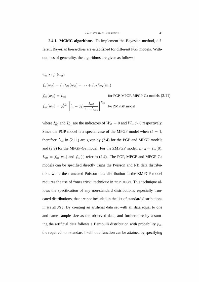
2.4. BAYESIAN INFERENCE 45
2.4.1. MCMC algorithms. To implement the Bayesian method, dif-
ferent Bayesian hierarchies are established for different PGP models. With-
out loss of generality, the algorithms are given as follows:
wit ∼ fit(wit)
fit(wit) = Ii1fit1(wit) + · · · + IiGfitG(wit)
fitl(wit) = Litl for PGP, MPGP, MPGP-Ga models (2.11)
fitl(wit) = φI∗it0t
[(1 − φt)
Litl
1 − Litl0
]I∗it1
for ZMPGP model
where I∗it0 and I∗it1 are the indicators of Wit = 0 and Wit > 0 respectively.
Since the PGP model is a special case of the MPGP model when G = 1,
therefore Litl in (2.11) are given by (2.4) for the PGP and MPGP models
and (2.9) for the MPGP-Ga model. For the ZMPGP model, Litl0 = fitl(0),
Litl = fitl(wit) and fitl(·) refer to (2.4). The PGP, MPGP and MPGP-Ga
models can be specified directly using the Poisson and NB data distribu-
tions while the truncated Poisson data distribution in the ZMPGP model
requires the use of “ones trick” technique in WinBUGS. This technique al-
lows the specification of any non-standard distributions, especially trun-
cated distributions, that are not included in the list of standard distributions
in WinBUGS. By creating an artificial data set with all data equal to one
and same sample size as the observed data, and furthermore by assum-
ing the artificial data follows a Bernoulli distribution with probability pit,
the required non-standard likelihood function can be attained by specifying

2.4. BAYESIAN INFERENCE 46
pit = fit(wit)/C in WinBUGS where C is a scaling constant to ensure all
pit < 1.
In order to construct the posterior density, some prior distributions are
assigned to the model parameters θ as follows:
βjkl ∼ N(0, τ 2jkl), j = µ, a; k = 0, 1, . . . , qj; l = 1, . . . , G (2.12)
φt ∼ Uniform(0, 1) for ZMPGP model (2.13)
rl ∼ Gamma(al, bl) for MPGP-Ga model (2.14)
π1 ∼ Uniform(0, 1) for MPGP, ZMPGP & MPGP-Ga models(2.15)
The prior specifications are mostly non-informative. For example, we set
the hyperparameter τ 2jkl = 1000. For the gamma distribution of the MPGP-
Ga model in (2.14), we set a1 = 7.5, a2 = 0.1 and bl = 10 based on the
information from the MPGP model that one group shows overdispersion
whilst another shows underdispersion in the new tumour counts. In case
of a G-group (G > 2) mixture model, the prior for π = (π1, . . . , πG) can
be replaced by the Dirichlet distribution Dir(α1, . . . , αG) where αl is set to
be 1/G. Note that I i = (Ii1, . . . , IiG) are not observed, thus a Bernoulli
distribution is assigned to Ii1 ∼ Bern(π1) or a multinomial distribution
I i ∼ multinomial(1, π1, . . . , πG) is assigned if G > 2. With the posterior
means Iil of the group membership indicators Iil, patient i is classified to
group l′ if Iil′ = maxlIil.

2.4. BAYESIAN INFERENCE 47
To implement the MCMC algorithms, we derive the conditional poste-
rior densities from which parameters are sampled. The conditional poste-
rior densities are proportional to the joint posterior density of complete data
likelihood and prior densities. Taking a 2-group ZMPGP model as an exam-
ple, the complete data likelihood is given by (2.8) and the priors are given
by (2.12), (2.13) and (2.15), hence treating Iil as missing observations, the
joint posterior density is
f(β,π,φ|w, I) ∝
m∏
i=1
(ni∏
t=1
φI∗it0t
)G∏
l=1
{πl
ni∏
t=1
[(1 − φt)
exp(−witl)(witl)wit
wit!(1 − exp(−witl))
]I∗it1}Iil
(∏
j=µ,a
1∏
k=0
G∏
l=1
fN(βjkl| 0, τ 2jkl)
)(10∏
t=1
fU(φt| 0, 1))fU(π1| 0, 1)
where fN(·| 0, τ 2jkl) represents a normal distribution with mean 0 and vari-
ance τ 2jkl, fU(·| 0, 1) denotes a uniform distribution on the interval [0, 1], w
is a vector of the data wit, I is a vector of Iil, β is a vector of βjkl and φ is a
vector φt. The univariate full conditional posterior densities for each of the
unknown model parameters θ = (β, π1,φ) and the latent group indicator
Ii1 are therefore given by:
f(βjkl|w, I,β−, π1,φ) ∝{
m∏
i=1
ni∏
t=1
[exp(−witl + βjklzjkitwit)
1 − exp(−witl)
]I∗it1(Iil)}
exp
(−β2
jkl
2τ 2jkl
),
j = µ, a; k = 0, 1; l = 1, 2
f(Ii1|w,β, π1,φ) ∝G∏
l=1
πl
ni∏t=1
(exp(−witl)w
wititl
1−exp(−witl)
)I∗it1
G∑l′=1
[πl′
ni∏t=1
(exp(−witl′ )w
wititl′
1−exp(−witl′ )
)I∗it1]
Iil
= Bernoulli(π′1)
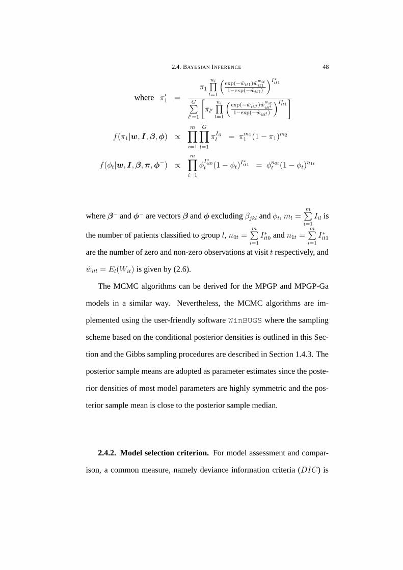
2.4. BAYESIAN INFERENCE 48
where π′1 =
π1
ni∏t=1
(exp(−wit1)w
witit1
1−exp(−wit1)
)I∗it1
G∑l′=1
[πl′
ni∏t=1
(exp(−witl′ )w
wititl′
1−exp(−witl′ )
)I∗it1]
f(π1|w, I,β,φ) ∝m∏
i=1
G∏
l=1
πIil
l = πm11 (1 − π1)
m2
f(φt|w, I,β,π,φ−) ∝m∏
i=1
φI∗it0t (1 − φt)
I∗it1 = φn0tt (1 − φt)
n1t
where β− and φ− are vectors β and φ excluding βjkl and φt, ml =m∑
i=1
Iil is
the number of patients classified to group l, n0t =m∑
i=1
I∗it0 and n1t =m∑
i=1
I∗it1
are the number of zero and non-zero observations at visit t respectively, and
witl = El(Wit) is given by (2.6).
The MCMC algorithms can be derived for the MPGP and MPGP-Ga
models in a similar way. Nevertheless, the MCMC algorithms are im-
plemented using the user-friendly software WinBUGS where the sampling
scheme based on the conditional posterior densities is outlined in this Sec-
tion and the Gibbs sampling procedures are described in Section 1.4.3. The
posterior sample means are adopted as parameter estimates since the poste-
rior densities of most model parameters are highly symmetric and the pos-
terior sample mean is close to the posterior sample median.
2.4.2. Model selection criterion. For model assessment and compar-
ison, a common measure, namely deviance information criteria (DIC) is

2.4. BAYESIAN INFERENCE 49
adopted. DIC originated by Spiegelhalter et al. (2002) is a Bayesian ana-
logue of Akaike’s Information Criterion (AIC) (Akaike, 1974). It is a mea-
sure of model fit and model complexity and has an advantage over the tradi-
tional AIC as it is not only applicable to nested models. DIC is composed
of the posterior mean devianceD(θ) which accounts for the fit of the model
and the effective dimension pD which assesses the complexity of the model.
For the PGP model, DIC is given by
DICM1 = D(θ) + pD
= − 4
M
M∑
j=1
m∑
i=1
ni∑
t=1
[I∗it ln fit(wit|θ(j))] + 2m∑
i=1
ni∑
t=1
I∗it ln fit(wit|θ)
where M is the number of realizations in the MCMC sampling algorithms,
θ(j) represents the vector of model parameter estimates under the j th simu-
lation in the posterior sample, θ is the vector of posterior means and fit(wit)
is a density function given by (2.4) with G = 1. DICM1 is output in
WinBUGS as it supports the calculation of DIC of the PGP model. Un-
fortunately the computation of DIC is infeasible for mixture models like
the MPGP (Model 2), ZMPGP (Model 3) and MPGP-Ga (Model 4) mod-
els. Applying the idea of Celeux et al. (2006), by considering Iil as missing
data, the complete DIC are defined for Model 2 to 4 respectively as fol-
lows:
For the MPGP and MPGP-Ga models,
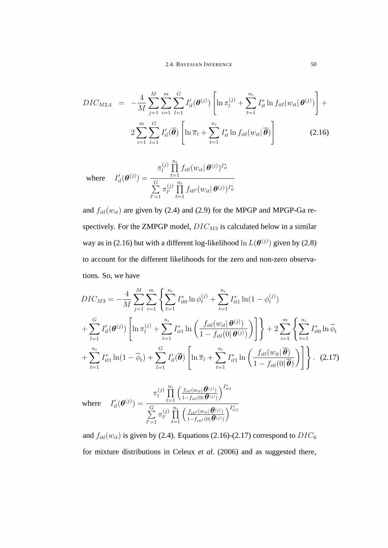
2.4. BAYESIAN INFERENCE 50
DICM2,4 = − 4
M
M∑
j=1
m∑
i=1
G∑
l=1
I ′il(θ(j))
[ln π
(j)l +
ni∑
t=1
I∗it ln fitl(wit|θ(j))
]+
2m∑
i=1
G∑
l=1
I ′il(θ)
[lnπl +
ni∑
t=1
I∗it ln fitl(wit|θ)
](2.16)
where I ′il(θ(j)) =
π(j)l
ni∏t=1
fitl(wit|θ(j))I∗it
G∑l′=1
π(j)l′
ni∏t=1
fitl′(wit|θ(j))I∗it
and fitl(wit) are given by (2.4) and (2.9) for the MPGP and MPGP-Ga re-
spectively. For the ZMPGP model, DICM3 is calculated below in a similar
way as in (2.16) but with a different log-likelihood lnL(θ(j)) given by (2.8)
to account for the different likelihoods for the zero and non-zero observa-
tions. So, we have
DICM3 = − 4
M
M∑
j=1
m∑
i=1
{ni∑
t=1
I∗it0 lnφ(j)t +
ni∑
t=1
I∗it1 ln(1 − φ(j)t )
+G∑
l=1
I ′il(θ(j))
[lnπ
(j)l +
ni∑
t=1
I∗it1 ln
(fitl(wit|θ(j))
1 − fitl(0|θ(j))
)]}+ 2
m∑
i=1
{ni∑
t=1
I∗it0 lnφt
+
ni∑
t=1
I∗it1 ln(1 − φt) +G∑
l=1
I ′il(θ)
[lnπl +
ni∑
t=1
I∗it1 ln
(fitl(wit|θ)
1 − fitl(0|θ)
)]}. (2.17)
where I ′il(θ(j)) =
π(j)l
ni∏t=1
(fitl(wit|θ(j))
1−fitl(0|θ(j))
)I∗it1
G∑l′=1
π(j)l′
ni∏t=1
(fitl′ (wit|θ(j))
1−fitl′ (0|θ(j))
)I∗it1
and fitl(wit) is given by (2.4). Equations (2.16)-(2.17) correspond to DIC6
for mixture distributions in Celeux et al. (2006) and as suggested there,

2.5. REAL DATA ANALYSIS 51
I ′il(θ(j)) is used in place of I (j)
il to save computing storage space. A model
with the smallest DIC is preferred as it indicates the chosen model has the
best fit of the data accounting for its complexity.
2.5. Real data analysis
In the bladder cancer study, we are interested in investigating the treat-
ment effect as well as the trend patterns of the patients’ tumour counts while
allowing for the population heterogeneity and excess zeros in the data. Ta-
ble 2.1 in Appendix 2.2 summarizes the parameter estimates and their stan-
dard errors (SE) (in italics) and model assessment measures for all fitted
models.
==================================
Table 2.1 about here
==================================
Starting from the simplest model, we first fitted the PGP model (Model
1). The mean function µit = exp(βµ0 + βµ1b) adopts ‘treatment’ (zµ1it =
b = 1, 2 to indicate ‘thiotepa’ and ‘placebo’ respectively) as a covariate
and the ratio function ait = exp(βa0 + βa1 t) adopts ‘time’ (za1it = t =
1, . . . , 10) as a time-evolving covariate. The time effect in the ratio func-
tion measures the change in trend direction, increasing or decreasing, over
time. As both the treatment and time effects are significant, they imply that
thiotepa treatment is associated with a decrease in new tumour count (95%
2.5. REAL DATA ANALYSIS 52
CI for βµ1:[−1.196,−0.6807]) and the new tumour count shows a decreas-
ing and then a slightly increasing trend (95% CI for βa0:[0.0368, 0.3075];
βa1:[−0.0298,−0.0020]).
Not surprisingly, patients with thiotepa treatment have lower tumour
counts in general. However within the treatment group, some of these pa-
tients had much higher counts (up to 9) while others had only zero counts
throughout the visiting period. To handle the population heterogeneity, we
postulate that there are two clusters of patients who responded differently
to the placebo treatment and the thiotepa treatment. We fitted the MPGP
model (Model 2) with the same set of covariates in the mean and ratio func-
tions. We have considered the quadratic effect of time and interaction effect
of time and treatment effect in the ratio function separately, but the parame-
ter estimates were found to be insignificant (95% CI contains zero) and were
discarded. Two clusters, namely the high-level and the low-level tumour
groups, are identified in which patient i is classified to group l, l = 1, 2 if
the posterior mean Iil = maxl′
Iil′ . The low-level (l = 1) group mainly con-
sists of patients with less than four tumour counts throughout the visiting
period whereas the high-level (l = 1) group contains patients with relatively
more tumours. Hence, the overdispersion in tumour counts amongst pa-
tients is captured by the mixture effect. The time effects (βa1l) in both ratio
functions are insignificant (95% CI contains zero) and hence are discarded.
After refitting the model, the low-level groups show a monotone decreas-
ing trend (95% CI for βa0l:[0.0392, 1.0350]) in new tumour counts over the

2.5. REAL DATA ANALYSIS 53
period of visits. Whereas the trend for the high-level group is stationary
(βa02:[−0.0143, 0.0658]). Moreover the treatment effect is significant (95%
CI for βµ12:[−0.8609,−0.2646]) only in the high-level group. These indi-
cate that the thiotepa treatment is ‘effective’ mainly for those patients with
higher level of new tumours.
Comparing the observed (80%) and the expected (67%) proportions of
zeros averaged over time, we find that the expected proportion is still much
lower than the observed one. This signifies that the MPGP model is inad-
equate in modelling the zero-inflation in the data. These zeros contribute
substantial noise in the detection of trends leading to insignificant time ef-
fects in both ratio functions. Hence despite the accommodation of popu-
lation heterogeneity by incorporating the mixture effect, the DIC for the
MPGP model does not show a great improvement.
To allow for zero-inflation, two models are considered, namely the ZMPGP
model (Model 3) and the MPGP-Ga model (Model 4) as the distribution of
both models give higher probabilities of zero counts than the Poisson dis-
tribution. Fitting a ZMPGP model using the hurdle approach is essentially
equivalent to remove all zero observations and model the non-zero obser-
vations using a zero-truncated distribution. Equivalently, the model is a
combination of a binary model to model the zero observations over the vis-
iting period and a MPGP model for the non-zero observations. Hence, this
model yields different results and interpretations from the MPGP model.

2.5. REAL DATA ANALYSIS 54
Under the ZMPGP model, after ignoring the zero observations, a major-
ity of 72 (88%) patients are classified to the low-level group, amongst them
34 (47%) patients received treatment. In this model, the treatment effect is
only significant in the low-level group (95% CI for βµ11:[−1.0870,−0.2996]).
The time effect in the ratio functions of both groups indicates the non-
monotone trends of new tumour counts prevail. In Appendix 2.3, Figure
2.1(a) shows the trends of new tumour counts given by (1 − φt)Witl where
Witl = El(Wit) in (2.6) for respectively the three groups, namely the high-
level (l = 2), the low-level without treatment (l = 1, b = 1) and the low-
level with treatment (l = 1, b = 1) groups, and Figure 2.1(b) reveals the
trends of individuals within each group. The predicted new tumour count
for patient i at time t is given by Wit = (1− φt)(Ii1Wit1 + Ii2Wit2
). Note
that the PGP model applies to discrete-time time series. However as we aim
to generalize the model to a continuous-time one, smoothing curves are thus
used to demonstrate the trend movements over a continuous time frame.
==================================
Figures 2.1(a) and 2.1(b) about here
==================================
Due to the fluctuating zero proportion over time, the expected new tu-
mour counts are fluctuating but the fluctuation is much less rigorous for
the low-level groups. In general, the new tumour counts for the high-level
group decline but rebound nearly to the starting level whereas those for the
low-level groups rise gently throughout but drop slightly near the end. The

2.5. REAL DATA ANALYSIS 55
wide gap of the new tumour counts between patients with and without treat-
ment shows that there is treatment effect in the low-level group. Trends in
both low- and high-level groups reveal that the condition of patients in the
high-level group deteriorates in the later half of the visiting period whereas
the treatment effect in the low-level groups starts with a lag. Since the
ZMPGP model performs much better in handling the zero-inflated data, the
DIC calculated using (2.17) decreases dramatically.
For the MPGP-Ga model, as it is capable of modelling overdispersed
count data, the low-level group (l = 1) shrinks to accommodate patients
essentially with zero observations throughout the study period. On the other
hand, the high-level group (l = 2) contains mainly patients with fluctuating
observations and hence accounts for most of the overdispersion in the new
tumour counts. Compared to the MPGP model, the MPGP-Ga model has
more distinct low-level and high-level groups. Overall, 46 patients (56%)
are classified into the high-level group with 16 of them (35%) receiving
treatment. Again in Appendix 2.3, Figure 2.2(a) reveals the predicted trends
of new tumour counts for respectively the three groups, namely the low-
level (l = 1), the high-level without treatment (l = 2, b = 1) and the
high-level with treatment (l = 1, b = 2) groups, and Figure 2.2(b) shows
the trends of individuals within each group. The predicted new tumour
count for patient i at time t is given by Wit = Ii1Wit1 + Ii2Wit2 where
Witl = El(Wit) is given by (2.10).

2.5. REAL DATA ANALYSIS 56
==================================
Figures 2.2(a) and 2.2(b) about here
==================================
Including zeros, differences across the three groups get wider for both
observed and expected levels of new tumour counts when compared to those
of the ZMPGP model. The low-level group contains patients with essen-
tially zero new tumour counts throughout the visiting period and hence the
treatment effect is insignificant in this group and is dropped thereafter. On
the contrary, for the high-level groups, the time effect (βa12 = −0.0137)
in the ratio function demonstrates a U-shaped trend pattern and represents
that the new tumour counts increase again after a gradual decline in the first
five visits. Again the wide gap in the levels between new tumour counts in
the high-level with and without treatment groups shows that there is signif-
icant treatment effect in this group (95% CI for βµ12:[−0.8318,−0.1357]).
These distinct trend patterns from the MPGP-Ga and ZMPGP models can
probably be explained by their different modelling approaches and resultant
classification.
Comparing to the ZMPGP model, there is an authentic decrease in the
DIC calculated using (2.16) for the MPGP-Ga model, despite the fact that
the expected proportion of zeros does not fit the observed one as good as in
the ZMPGP model. The better DIC can be explained by the brevity and
flexibility in the pmf of the MPGP-Ga model to handle overdispersion and
thus it gives a better fit to the data.
2.5. REAL DATA ANALYSIS 57
Finally we conclude the performances of the proposed models to han-
dle excess zero and overdispersion by plotting the expected proportions of
zeros p0t and expected variances vt, over time with the observed propor-
tions of zeros P0t and observed variances Vt in Figures 2.3(a) and 2.3(b) in
Appendix 2.3. The observed proportions of zeros and variances are simply
calculated based on the observed data for each time t and are constant across
models. The expected proportions of zeros p0t are expressed as a weighted
average of the probability of getting zero based on different densities over
each treatment and mixture subgroup, where the weights are the sum of the
mixture group indicators of the patients∑
i
Iil in the subgroups. The ex-
pected variances vt are also computed as weighted averages of the variance
of each treatment and mixture groups. In particular, if there are two mixture
groups in Model 2 to 4, the variance vt comprises of the variance of expec-
tation and the expectation of variance conditional on the mixture group l,
that is we get the weighted average within the mixture group using πl before
calculating the overall expected variances. In other words,
vt =1
m
[m∑
i=1
I(zµ1i = 1)v1t +m∑
i=1
I(zµ1i = 2)v2t
](2.18)
vbt =G∑
l=1
πl
[V arl(Wit) + El(W
2it)]−[
G∑
l=1
πlEl(Wit)
]2
, b = 1, 2 (2.19)
where the mean El(Wit) and variance V arl(Wit) conditional on group l are
given by (2.1) and (2.10) for the MPGP and MPGP-Ga models respectively.
For the ZMPGP model, vbt = V ar(Wit) is given by (2.7) when zµ1i = b.
2.6. DISCUSSION 58
==================================
Figures 2.3(a) and 2.3(b) about here
==================================
Figure 2.3(a) shows that, across Model 1 to Model 4, the expected pro-
portions of zeros p0t increase in general and approach those of the observed
proportions P0t, with those of ZMPGP model being the best because φt is
indeed estimated by P0t at each time t. Hence the models are becoming
more and more capable of handling excess zero which is the first focus of
this Chapter. The second focus concerns the overdispersion of the data. Fig-
ure 2.3(b) shows that the observed and expected variances under different
models are more deviated. While Model 1 and 2 are still inefficient to han-
dle overdispersion, the performance of the MPGP-Ga model and ZMPGP
model are much more satisfactory.
2.6. Discussion
Motivated by the bladder cancer data and the limited literature in mod-
elling zero-inflated and overdispersed longitudinal time series of counts, we
extend, in this Chapter, the MPGP model of Chan & Leung (2010) which
cannot cope with excess zeros and substantial overdispersion. As the blad-
der cancer data from longitudinal measurements have substantial population
heterogeneity, we first extend the PGP model to incorporate mixture effect
and the resultant MPGP model is capable of distinguishing two groups of
patients with very different trends of new tumour counts. At the same time,

2.6. DISCUSSION 59
zero-inflation is another problem in the data which seriously affects the pre-
diction of trend patterns in the data. Hence, we develop two distinct models,
namely the ZMPGP model and MPGP-Ga model to handle such problem.
The ZMPGP model is essentially a mixture of zero-degenerated model and
a zero-truncated MPGP model via the hurdle approach, while the MPGP-
Ga model is a state space model with state variable El(Wit) = Xitl where
Xitl follows a gamma distribution.
It should be noted that while both ZMPGP and MPGP-Ga models are
suitable for modelling data with overdispersion and excess zeros, they are
not built to cater for serial correlation in the time series. This is because the
data contains too many missing observations such that the autoregressive
terms cannot be defined for a substantial portion of time points in the time
series of most patients. Hence the OD and PD approaches of the popular
panel count models reviewed in Chapter 1 are not considered here.
For model implementation, we adopt the Bayesian method with MCMC
techniques by using WinBUGS. The models are assessed and compared
through a popular criterionDIC which measures the fit of the model taking
into account the model complexity. Results show that the ZMPGP model,
though gives a substantial drop in DIC when compared with the MPGP
model, is not as good as the MPGP-Ga model after model complexity is
also taken into consideration.
In conclusion, the two target models, MPGP-Ga and ZMPGP have dif-
ferent performance and interpretation. The MPGP-Ga model has largest

2.6. DISCUSSION 60
variances in general because of the extra variability from the stochastic
GP in the mean of Poisson distribution. The ZMPGP model also has rela-
tively large variances due to the zero-truncated Poisson distribution. While
other models still have relatively smaller variances, the MPGP-Ga model
and ZMPGP model are more suitable for data with overdispersion. For
zero-inflation, the two models handle the problem in a different way and
therefore are suitable under different situations. In a medical context, the
ZMPGP model recognizes the development of new tumours as a two-stage
disease progression. The binary model decides whether the patients are at
carcinogenic risk of recurrence of tumours. If they suffer from recurrence
(Wit > 0), the truncated Poisson model describes the subsequent trends
which is usually of more clinical interest. On the contrary, if the zero obser-
vations reveal important information for treatment outcomes, the MPGP-Ga
model is perhaps more appropriate.
Our study also gives us insight on the existence of non-monotone trend
of new tumour counts. Both ZMPGP and MPGP-Ga models suggest that
there is a possibility of resurgence of tumours across the visiting period
despite the use of thiotepa. Therefore, clinicians should exercise some pre-
cautionary measures, such as dosage increment, to inhibit the resurrection
of the tumours.
Lastly, there are 37% of missing data and they are simply ignored in
the models by implicitly assuming that the missing are completely random.
This assumption may be invalid as experiences in clinical trials show that

2.6. DISCUSSION 61
such dropouts are often nonignorable. Hence one possible remedy in this
data analysis is to set up a dropout model to allow for the dropout effect on
the treatment outcomes.

2.6. DISCUSSION 62
Appendix 2.1Number of new tumours found in 82 patients taking placebo and thiotepa treatments in the bladder cancer study
Placebo: Visit (months)Patient 3 6 9 12 15 18 21 24 27 30
1 0 - - - - - - - - -2 - 0 - - - - - - - -3 0 - 0 - - - - - - -4 0 1 0 - - - - - - -5 0 - 0 - 0 - - - - -6 0 - 0 2 3 0 - - - -7 0 - - - 0 0 - - - -8 - 2 0 0 - 0 - - - -9 0 0 6 - 3 0 - 0 - -10 8 - 0 0 8 0 - 8 - -11 1 0 1 0 0 0 8 0 - -12 0 0 0 0 0 0 - 0 - -13 0 8 7 0 5 - - 7 - -14 1 0 0 0 1 0 0 3 - -15 8 0 - 0 0 0 0 0 0 -16 4 0 - - - - - - 8 -17 0 0 - 0 0 - 0 0 0 -18 - 0 - - - - - 3 0 -19 - 0 0 - - 0 - - - 020 0 0 - - 0 - - - - 021 0 0 0 0 - 0 - 0 - 022 4 - 0 - - 2 4 0 0 023 1 3 3 3 0 0 0 0 3 024 0 0 0 0 - - 0 - 2 125 0 0 0 2 3 0 - 1 0 026 0 0 0 0 0 0 0 - 0 -27 0 - 0 - 0 - 0 - - 028 0 0 0 0 0 0 0 0 - 029 - - 0 - - - 0 - - 830 0 - 0 - - 0 - 0 - 031 0 - 8 - 0 2 5 1 0 032 0 0 0 0 0 9 - 1 0 233 0 0 0 0 0 0 0 0 0 034 3 0 0 - 0 - 0 - 0 035 0 1 0 0 0 0 0 0 - -36 5 3 4 - 0 0 0 0 0 037 0 0 1 3 - 0 1 0 4 338 0 0 0 0 0 1 0 0 0 039 - 0 0 0 - 0 - 0 - 040 0 0 - 0 - 0 - 0 - 041 0 - 0 0 0 1 0 0 0 042 7 - - 0 2 - - - 0 043 0 0 0 0 0 0 0 - 0 -44 1 0 0 0 3 0 - 4 0 345 0 3 0 0 4 0 2 0 5 046 1 0 3 6 - 4 1 0 0 0

2.6. DISCUSSION 63
Thiotepa:
Visit (months)Patient 3 6 9 12 15 18 21 24 27 30
47 - 8 - - - - - - - -48 0 0 0 - - - - - - -49 - 0 0 - - - - - - -50 0 - - 0 - - - - - -51 1 0 0 0 0 - - - - -52 7 7 2 0 0 0 - - - -53 - 0 - 0 - 2 - - - -54 - - - - - 0 - - - -55 2 - - - - 0 - - - -56 0 0 0 0 0 2 0 - - -57 0 0 0 - 0 0 0 - - -58 0 - 0 0 - 0 0 0 - -59 - - 0 0 - 0 - 0 - -60 0 0 0 0 0 0 0 0 - -61 0 2 0 3 - - 1 0 0 -62 0 1 0 0 0 - 0 - 0 -63 2 - - - - - - - - 064 0 0 0 - - - 0 0 3 065 0 0 0 0 0 0 0 0 0 -66 0 1 0 0 3 0 0 3 3 067 0 0 0 0 0 0 2 1 2 -68 - 0 - - 0 0 - 3 2 169 0 0 0 0 0 0 0 0 0 070 0 0 0 0 0 0 0 0 0 071 1 0 - 0 - 0 0 0 1 072 - - 0 - - - - 0 - -73 2 0 0 0 0 0 1 2 1 074 0 0 0 0 0 - 0 0 0 -75 1 0 0 0 0 0 0 0 0 -76 0 0 0 0 0 0 0 0 0 077 - - - 0 0 - - 0 - 078 1 - 0 0 - - 0 1 - 079 0 - - - - - 0 0 - -80 0 0 0 0 0 0 0 0 0 081 0 0 0 0 0 0 0 0 0 082 0 0 0 0 0 0 0 0 0 0
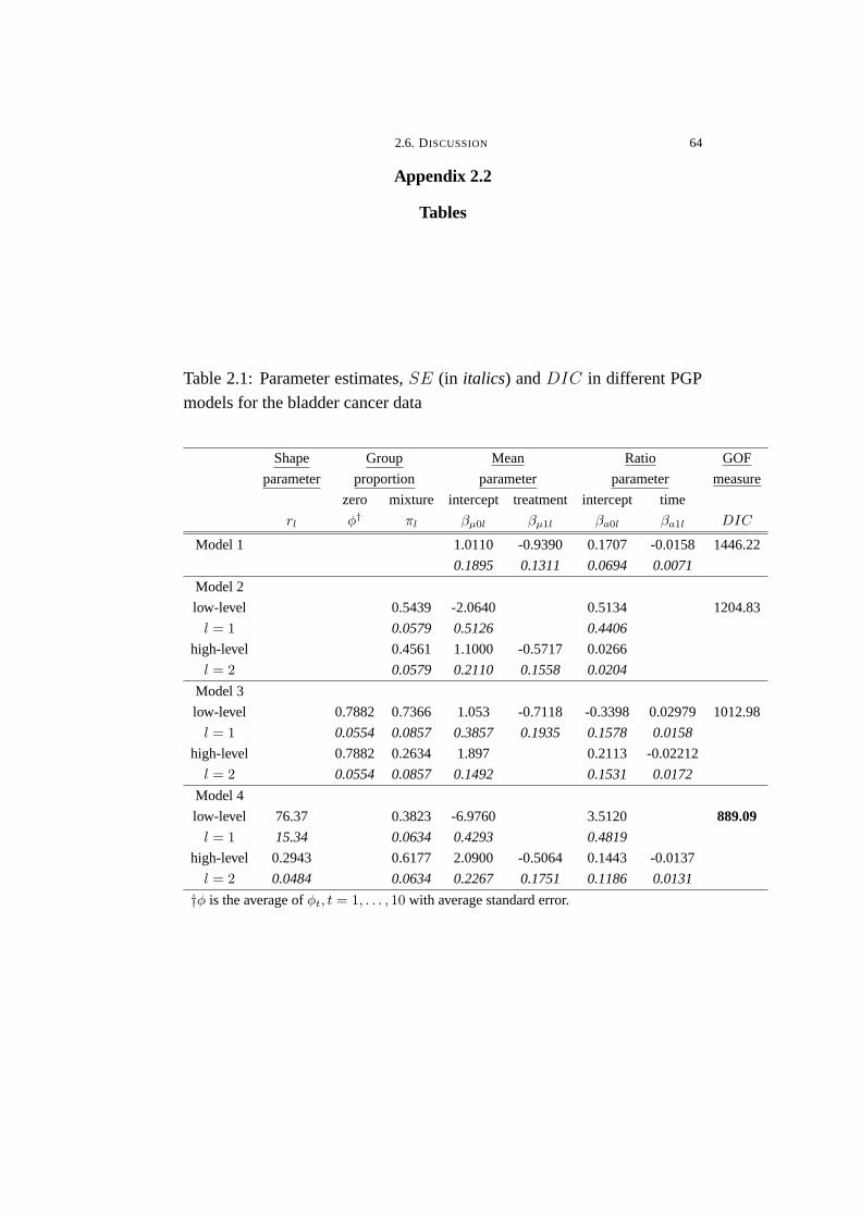
2.6. DISCUSSION 64
Appendix 2.2
Tables
Table 2.1: Parameter estimates, SE (in italics) and DIC in different PGP
models for the bladder cancer data
Shape Group Mean Ratio GOF
parameter proportion parameter parameter measure
zero mixture intercept treatment intercept time
rl φ† πl βµ0l βµ1l βa0l βa1l DIC
Model 1 1.0110 -0.9390 0.1707 -0.0158 1446.22
0.1895 0.1311 0.0694 0.0071
Model 2
low-level 0.5439 -2.0640 0.5134 1204.83
l = 1 0.0579 0.5126 0.4406
high-level 0.4561 1.1000 -0.5717 0.0266
l = 2 0.0579 0.2110 0.1558 0.0204
Model 3
low-level 0.7882 0.7366 1.053 -0.7118 -0.3398 0.02979 1012.98
l = 1 0.0554 0.0857 0.3857 0.1935 0.1578 0.0158
high-level 0.7882 0.2634 1.897 0.2113 -0.02212
l = 2 0.0554 0.0857 0.1492 0.1531 0.0172
Model 4
low-level 76.37 0.3823 -6.9760 3.5120 889.09l = 1 15.34 0.0634 0.4293 0.4819
high-level 0.2943 0.6177 2.0900 -0.5064 0.1443 -0.0137
l = 2 0.0484 0.0634 0.2267 0.1751 0.1186 0.0131
†φ is the average of φt, t = 1, . . . , 10 with average standard error.
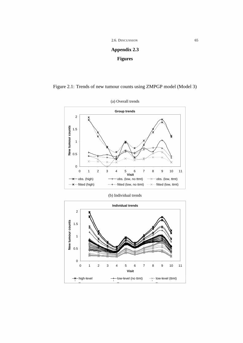
2.6. DISCUSSION 65
Appendix 2.3
Figures
Figure 2.1: Trends of new tumour counts using ZMPGP model (Model 3)
(a) Overall trends
Group trends
0
0.5
1
1.5
2
0 1 2 3 4 5 6 7 8 9 10 11Visit
New
tu
mo
ur
cou
nts
obs. (high) obs. (low, no ttmt) obs. (low, ttmt)
fitted (high) fitted (low, no ttmt) fitted (low, ttmt)
(b) Individual trends
Individual trends
0
0.5
1
1.5
2
0 1 2 3 4 5 6 7 8 9 10 11
Visit
New
tu
mo
ur
cou
nts
high-level (no ttmt) high-level (ttmt) low-level_ _ _
Individual trends
0
0.5
1
1.5
2
0 1 2 3 4 5 6 7 8 9 10 11
Visit
New
tu
mo
ur
cou
nts
high-level low-level (no ttmt) low-level (ttmt)_ _ _

2.6. DISCUSSION 66
Figure 2.2: Trends of new tumour counts using MPGP-Ga model (Model 4)
(a) Overall trends
Group trends
0
0.5
1
1.5
2
0 1 2 3 4 5 6 7 8 9 10 11Visit
New
tu
mo
ur
cou
nts
obs. (high,no ttmt) obs. (high,ttmt) obs. (low)
fitted (high,no ttmt) fitted (high,ttmt) fitted (low)
(b) Individual trends
Individual trends
0
0.5
1
1.5
2
0 1 2 3 4 5 6 7 8 9 10 11
Visit
New
tu
mo
ur
cou
nts
high-level (no ttmt) high-level (ttmt) low-level_ _ _

2.6. DISCUSSION 67
Figure 2.3: Proportions of zeros and variances of new tumour counts for
Model 1 to 4
(a) proportions of zeros across time
Proportion of zeros
0.4
0.5
0.6
0.7
0.8
0.9
1
0 1 2 3 4 5 6 7 8 9 10 11Visit
Pro
po
rtio
n o
f ze
ros
Observed Model 1 Model 2 Model 3 Model 4
(b) variances across time
Proportion of zero
0.4
0.5
0.6
0.7
0.8
0.9
1
0 1 2 3 4 5 6 7 8 9 10 11Visit
Pro
po
rtio
n o
f ze
ro
Observed Model 1 Model 2 Model 3 Model 4
Variance
0
1
2
3
4
5
0 1 2 3 4 5 6 7 8 9 10 11
Visit
Var
ian
ce
Observed Model 1 Model 2 Model 3 Model 4

CHAPTER 3
Robust Poisson geometric process model
Continued from the development of PGP models to allow for overdis-
persion due to zero-inflation by the ZMPGP model in (2.4) and MPGP-Ga
model (2.9), this Chapter focuses on accommodating overdispersion due to
outlying observations.
3.1. Background
Most time series measured over continuous range assume a normal error
distribution. These traditional time series models are however vulnerable to
outliers. Outliers in time series have been realized as an influential factor
in model fitting and forecasting. Failure to downweigh the outlying effects
may lead to a poor model fit, an overestimation of variance, an inappropri-
ate interpretation and an inaccurate prediction. This issue has received a
great deal of attention, therefore several approaches have been developed to
reduce the influence of outliers and the distributional deviation in the data
analysis. In the past, two main approaches have been considered to cope
with the overdispersion caused by the outliers. The first approach simply
incorporates mixture effects to account for the heterogeneity in the distri-
bution of the data. This can be viewed as a missing data problem assuming
that the membership of the data from one of the distributions is unknown
68
3.1. BACKGROUND 69
and has to be estimated. The mixture model is usually implemented using
expectation-maximization (EM) algorithm or Markov chain Monte Carlo
(MCMC) sampling algorithm.
The second approach is to adopt a heavy-tailed distribution instead of
the commonly used Gaussian distribution as the error distribution of the
data. Some popular choices of heavy-tailed distributions include the Stu-
dent’s t-distribution and a more general class of distributions is the Pear-
son Type IV distribution (Johnson et al., 1995). Alternatively, the expo-
nential power (EP) distribution which can describe a leptokurtic (positive
excess kurtosis) or platykurtic (negative excess kurtosis) shape is another
good choice. However, in the context of Bayesian analysis, the implemen-
tation of these distributions is troublesome because the marginal posterior
distributions of the parameters are difficult to derive using conventional nu-
merical and analytic approximations (Choy & Smith, 1997). To overcome
this problem, Box & Tiao (1973) proposed a new exponential power family
of normal scale mixtures (SMN) and later Qin et al. (1998) pioneered the
scale mixtures of uniforms (SMU) which replaces the normal distribution
in the SMN form by uniform distribution. Theoretically, any distribution
that can be expressed by SMN form, also has a SMU representation.
The hierarchical structure of the SMN or SMU representation possesses
two prominent advantages: (1) the resulting density contains a mixing pa-
rameter which can accommodate the extra-Poisson variation and help to

3.1. BACKGROUND 70
identify the extreme values in outlier diagnosis and (2) the parameter esti-
mation can be simplified by sampling from normal or uniform distribution
using MCMC algorithms such as Gibbs sampling. The recent emergence
of the software WinBUGS which performs Bayesian statistical inferences
using MCMC algorithms also facilitates the implementation of these repre-
sentations, thus enhancing their popularity in the context of Bayesian mod-
elling. This hierarchical structure is very practical in insurance applications
because it is well known that the normal error distribution falls short of
allowing for irregular and extreme claims and hence contaminates the es-
timation procedure and leads to poor estimation. For instances, Choy &
Chan (2003) applied the Student’s t- and EP distributions in scale mixtures
(SM) representations to predict the insurance premiums to be charged on
the policyholders in credibility analysis and Chan et al. (2008) predicted
and projected the loss reserves data with various heavy-tailed distributions
under the generalized-t distribution family expressed in SMU representa-
tion.
So far, the techniques of using scale mixtures representation apply solely
to continuous time series. Yet, discrete count time series is observed in
many occasions especially in a medical context. In clinical trials where the
measurements are usually longitudinal, sometimes the appearance of outly-
ing observations may inflate the mean and variance of the data distribution
and have an adverse effect on both the parameter estimation and predic-
tion. Despite overdispersion caused by outlying observations, trend, cluster

3.1. BACKGROUND 71
effect and serial correlation are often detected in longitudinal count time
series. Examining the trend patterns is particularly important as it provides
useful information on the movement of outcomes over time.
To cope with overdispersion, clustering as well as serial correlation,
Thall & Vail (1990) proposed adding subject-specific and time-specific ran-
dom effects into the mean link function to give extra Poisson-variation to the
outcomes. Assume that the outcome Wit follows a Poisson distribution, xit
and β are vectors of time-evolving covariates and regression coefficients,
{γi, i = 1, ,m} are positive-valued subject-specific random effects which
are independently distributed and {ut, t = 1, . . . , n} are positive-valued
time-specific random effects which are independently and identically dis-
tributed. Under the GLMM framework, Thall & Vail (1990) showed that
the marginal moments for Wit are given by
E(Wit) = exp(xTitβE[ln(γiut)])
V ar(Wit) = exp(xTitβ) +
{V ar(γi)
[E(γi)]2+V ar(ut)
[E(ut)]2
}[exp(xT
itβ)]2
Cov(Wit,Wi,t−k) =V ar(γi)
[E(γi)]2exp(xT
itβ) exp(xTi,t−kβ).
However, Jowaheer & Sutradhar (2002) pointed out that the above model is
unable to accommodate autocorrelation structures such as the first-order au-
toregressive (AR(1)) structure. Therefore he considered a Poisson-gamma
mixed model to allow for overdispersion and incorporated an autoregres-
sive (AR) structure to the outcome to accommodate serial correlation. His
model is essentially a negative binomial model and can be classified as a

3.1. BACKGROUND 72
OD model as the current outcome depends on past observations. Neverthe-
less, their models have not put much emphasis on investigating the trend
movements and the mixed model approach which assumes the mean of the
Poisson distribution follows gamma or log-normal distribution may be in-
adequate to cast light on the outlying effect caused by the extreme obser-
vations. To tackle this pitfall, plenty of studies considered various mix-
ing distributions. Some useful ones include generalized inverse Gaussian,
generalized gamma, generalized exponential, inverse gamma, etc. Refer to
(Gupta & Ong, 2005) for more details.
In this Chapter, we seek a new direction to model overdispersed longitu-
dinal time series of counts due to the presence of outliers while allowing for
non-monotone trends, cluster effect and serial correlation. Our proposed
model is an extension of the mixture Poisson geometric process (MPGP)
model introduced by Chan et al. (2010b) and Wan (2006) and a modifica-
tion of the MPGP-Ga model in the last Chapter by replacing the gamma
distribution with some heavy-tailed distributions in SM representation. The
resultant model is named as the robust mixture Poisson geometric process
(RMPGP) model. In the RMPGP model, we assume that the outcome vari-
able has a Poisson distribution with a stochastic mean which forms a latent
GP, and the mean of the GP after geometrically discounted by the ratio fol-
lows a heavy-tailed distribution such as log-t distribution or log-exponential
power (log-EP) distribution represented in SMN and SMU forms respec-
tively. Under the SM representation, the model parameters can be simulated

3.1. BACKGROUND 73
using MCMC algorithms and the mixing parameters help to identify the ex-
treme values in outlier diagnosis. To our knowledge, this is a pioneering
work in adopting Student’s t- and EP distributions as mixing distributions
for time series of counts. Moreover, our proposed GP models have a trend
component (ratio function) which enables the study of trend movements and
can accommodate cluster effect using a mixture of robust Poisson geometric
process (RPGP) models. These make the RPGP models more advantageous
than many existing time series models for count data.
To demonstrate the characteristics and application of our models, the
rest of the Chapter is presented as follows. First, the development of RPGP
and RMPGP models using Student’s t- and EP distributions from the PGP
model will be described in Section 3.2. Section 3.3 will introduce the SM
representation of the two heavy-tailed distributions and their implementa-
tion in the RMPGP model. Besides, the hierarchical structure and MCMC
algorithms of the models will be given followed by the introduction of the
model assessment criterion and a test for serial correlation. Furthermore,
Section 3.4 will investigate the properties of the RMPGP models through
a simulation study and Section 3.5 will demonstrate an application of the
proposed models using the epilepsy data studied by Leppik et al. (1985)
with discussion. Lastly, a brief summary will be given in Section 3.6.
3.2. MODEL SPECIFICATION 74
3.2. Model specification
This Section first introduces the general framework of the RPGP model.
Then the proposed model using two commonly used heavy-tailed distri-
butions will be discussed with an examination of the model distributions.
After that, the incorporation of mixture effect will be described briefly.
3.2.1. RPGP Model. LetWit denotes the outcome for subject i at time
twhere i = 1, . . .m, t = 1, . . . , ni and n =m∑
i=1
ni. Assume thatWit follows
a Poisson distribution fP (wit|xit) with mean Xit which forms a latent GP.
Furthermore, the stochastic process {Yit = at−1it Xit, t = 1, . . . , ni} follows
some lifetime distributions f(yit), such as exponential distribution in Wan
(2006) and gamma distribution in Chapter 2, with mean E(Yit) = µit, the
resultant model is called Poisson geometric process (PGP) model.
Without loss of generality, we assume that the logarithm of Yit, i.e.
Y ∗it = lnYit follows a heavy-tailed distribution f(y∗it) with mean E(Y ∗
it ) =
µ∗it. Then, the marginal pmf for Wit is
f(wit) =
∫ ∞
0
fP
(wit
∣∣∣∣ey∗
it
at−1it
)f(y∗it) dy
∗it
=
∫ ∞
0
exp(− ey∗it
at−1it
)(ey∗it
at−1it
)wit
wit!f(y∗it) dy
∗it. (3.1)
The resultant model is named as the robust Poisson GP (RPGP) model.
The RPGP model is essentially a state space model with state variables
Xit and has time-evolving mean and ratio functions to accommodate ex-
ogenous effects and non-monotone trends. The mean function µ∗it which is
3.2. MODEL SPECIFICATION 75
identity-linked and ratio function ait which is log-linked to linear functions
of covariates are defined as:
µ∗it = βµ0 + βµ1zµ1it + · · · + βµqµ
zµqµit (3.2)
ln ait = βa0 + βa1za1it + · · · + βaqazaqait (3.3)
where zjkit, j = µ, a; k = 1, . . . , qj are some time-evolving covariates.
By mixing the Poisson distribution with some heavy-tailed distribu-
tions, extra variability is added to the Poisson distribution which enables
the model to accommodate the inflated variance caused by some extreme
observations. In this Chapter, we consider the Student’s t- and EP distribu-
tions because they have different shapes including heavier-than-normal to
normal tails in the former as well as platykurtic shape and leptokurtic shape
with a kink in the latter. The various shapes allow the model to be more
flexible to capture different kurtoses in the data.
3.2.1.1. RPGP model with Student’s t-distribution. If Y ∗it has a Stu-
dent’s t-distribution with mean µ∗it and variance
ν
ν − 2σ2, the probability
density function of Student’s t-distribution fT (y∗it) is given by
fT (y∗it) =Γ(ν+1
2)√
νπσΓ(ν2)
[1 +
(y∗it − µ∗it)
2
νσ2
]− (ν+1)2
(3.4)
where µ∗it is given by (3.2) and ν > 2 is the degrees of freedom which
controls the tailedness. A small ν gives a heavier tail and Student’s t-
distribution converges to normal distribution when ν → ∞. The kurtosis
is6
ν − 4+ 3 for ν > 4 which is greater than 3, the kurtosis of the normal
distribution.

3.2. MODEL SPECIFICATION 76
To study the pmf of the proposed RPGP-t model, we assume qµ = qa =
1, zµ1 = b = 0, 1 as the covariate effect and za1t = t as the time-evolving
effect in (3.2) and (3.3). Hence the mean function µt = exp(βµ0 + βµ1b)
and ratio function at = exp(βa0 +βa1t). Fixing b = 1 and t = 2, we change
the values of one of the scale σ, shape ν or location parameters βa0 and βµ0
each time while keeping the other parameters constant and approximate
the pmf in (3.1) using Monte Carlo (MC) integration as described below.
Conditional on covariate zµ1 = b and time t, the marginal pmf estimator
fbt(w), in general, can be obtained by:
fbt(w) =Ms∑
j=1
fP
(w
∣∣∣∣∣ey
∗(j)bt
at−1t
)=
Ms∑
j=1
exp
(− e
y∗(j)bt
at−1t
)(ey∗(j)bt
at−1t
)w
w!, w = 0, 1, . . . ,∞; and
y∗(j)bt ∼ fT (y
∗(j)bt |µ∗
t , σ, ν), j = 1, . . . ,Ms (3.5)
whereMs = 10000 is the number of simulations and the latent y∗(j)bt are sim-
ulated from the Student’s t-distribution in (3.4) given the parameters µ∗it, σ
and ν. Besides examining the mean and variance, we also study the kurtosis
of the approximated pmf using the method in Gupta & Ong (2005) for a dis-
crete distribution. The relative long-tailedness of the distribution is defined
as limw→∞fbt(w + 1)
fbt(w)where the limit is zero for Poisson distribution. By
fixing the parameters at ν = 10, σ = 0.5, βµ0 = 3.0, βµ1 = −0.2, βa0 = 0.5
and βa1 = −0.1 but leaving one floating, the marginal pmfs are displayed
in Figures 3.1(a) to 3.1(d) in Appendix 3.3 with their means, variances and
kurtoses summarized in Table 3.1 in Appendix 3.2. Note that since different

3.2. MODEL SPECIFICATION 77
pmfs are drawn on the same graph for comparison, we use curves instead
of bars to represent the marginal pmfs for better visualization.
====================================
Figures 3.1(a) to 3.1(d) and Table 3.1 about here
====================================
Results from Figures 3.1(a) to 3.1(d) reveal that in general the loca-
tion, variability and tailedness of the marginal pmf depend on parameters
βjk, j = µ, a; k = 0, 1, in which a larger βµ0 and a smaller βa0 lead to larger
mean, variance and kurtosis. Whereas, ν and σ control the spread and the
tail behaviour of the distribution without altering its mean. A smaller ν and
a larger σ contribute to a larger variability and a heavier tail and thus the
model can accommodate the outlying effect due to extreme values while
keeping the mean unchanged. Since the variance of each distribution in
Table 3.1 is substantially larger than the mean, the RPGP-t model is capa-
ble of fitting data with overdispersion due to outliers as well as data with
equidispersion when σ is small.
3.2.1.2. RPGP model with EP distribution. If Y ∗it has an exponential
power (EP) distribution, also known as generalized error distribution, with
mean µ∗it and variance σ2, it has a probability density function
fEP (y∗it) =c1σ
exp
−∣∣∣∣∣c1/20 (y∗it − µ∗
it)
σ
∣∣∣∣∣
2/ν (3.6)
where c0 =Γ(3ν/2)
Γ(ν/2), c1 =
c1/20
(νΓ(ν/2))and ν ∈ (0, 2] is a shape parameter
which controls the kurtosis. This family subsumes a range of symmetric

3.2. MODEL SPECIFICATION 78
distributions such as uniform (ν → 0) with kurtosis equal to 1.8, normal
(ν = 1) with kurtosis equal to 3 and double exponential (ν = 2) with
a kurtosis of 6. Its tails can be more platykurtic when ν < 1 or more
leptokurtic when ν > 1 compared with the normal tail (ν = 1).
By fixing the parameters at ν = 1, σ = 0.5, βµ0 = 3.0, βµ1 = −0.5, βa0 =
0.5 and βa1 = −0.1 but leaving one floating, the marginal pmfs are again
approximated using MC integration specified in (3.5) but replacing fT (y∗(j)bt |µ∗
t , σ, ν)
with fEP (y∗(j)bt |µ∗
t , σ, ν) in (3.6). The effects of different parameters on
the resulting pmfs are illustrated in Table 3.2 in Appendix 3.2 and Figures
3.2(a) to 3.2(d) in Appendix 3.3. Clearly, the tail of the distribution depends
on all the parameters and the behaviours of the parameters σ, βµ0 and βa0 on
the resultant pmf are quite close to that of RPGP-t model. However, com-
paring Figure 3.2(a) with Figure 3.1(a), the shape parameter ν in the RPGP-
EP model allows a wider range of shapes than that of the RPGP-t model as
the EP distribution includes both leptokurtic and platykurtic shapes. Hence
the RPGP-EP model can accommodate different degrees of tailedness due
to moderate to adverse outlying effects.
====================================
Figures 3.2(a) to 3.2(d) and Table 3.2 about here
====================================
3.2.2. Incorporation of mixture effects. Overdispersion may arise due
to cluster effect, hence an alternative way to tackle overdispersion is to add
mixture effects into the mean and ratio functions. Suppose that there are G
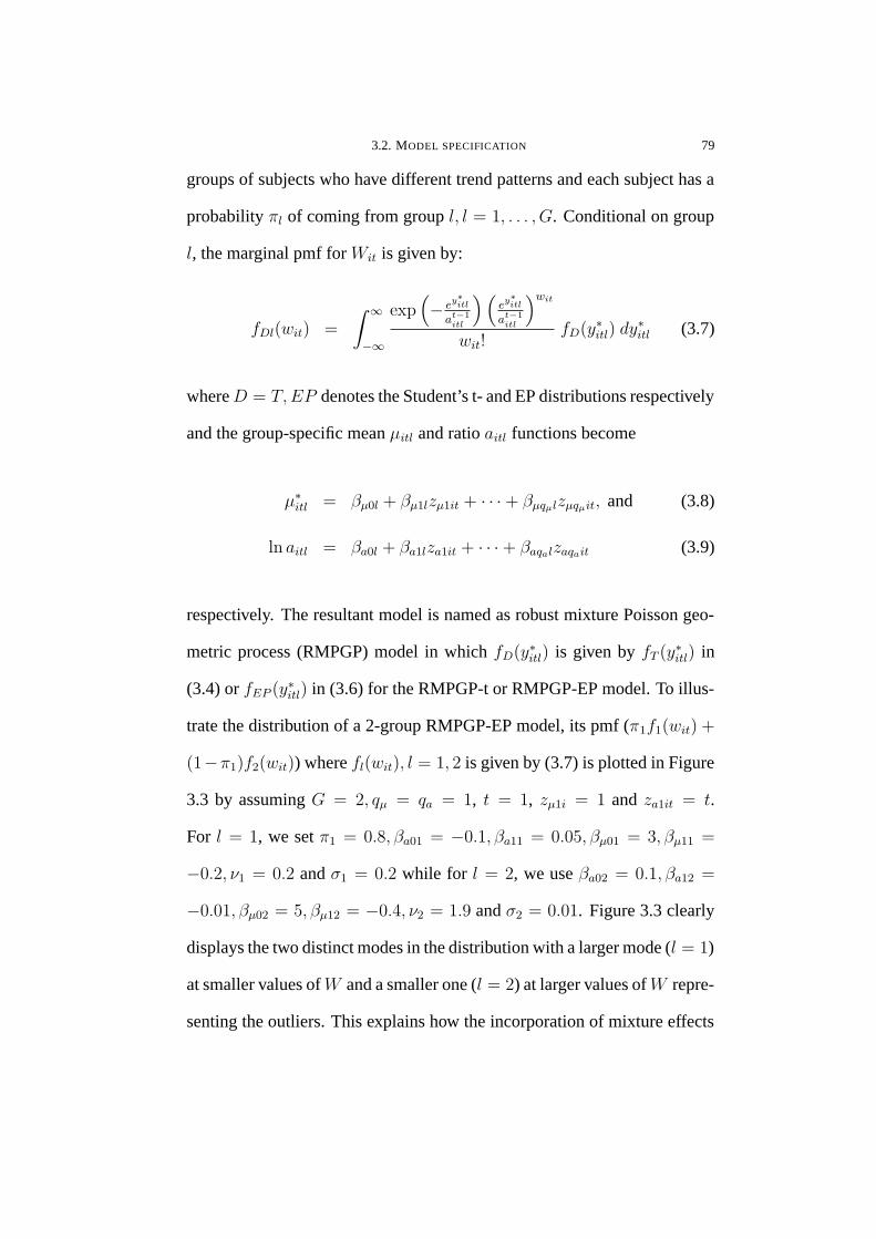
3.2. MODEL SPECIFICATION 79
groups of subjects who have different trend patterns and each subject has a
probability πl of coming from group l, l = 1, . . . , G. Conditional on group
l, the marginal pmf for Wit is given by:
fDl(wit) =
∫ ∞
−∞
exp(− ey∗
itl
at−1itl
)(ey∗
itl
at−1itl
)wit
wit!fD(y∗itl) dy
∗itl (3.7)
whereD = T,EP denotes the Student’s t- and EP distributions respectively
and the group-specific mean µitl and ratio aitl functions become
µ∗itl = βµ0l + βµ1lzµ1it + · · · + βµqµlzµqµit, and (3.8)
ln aitl = βa0l + βa1lza1it + · · · + βaqalzaqait (3.9)
respectively. The resultant model is named as robust mixture Poisson geo-
metric process (RMPGP) model in which fD(y∗itl) is given by fT (y∗itl) in
(3.4) or fEP (y∗itl) in (3.6) for the RMPGP-t or RMPGP-EP model. To illus-
trate the distribution of a 2-group RMPGP-EP model, its pmf (π1f1(wit) +
(1−π1)f2(wit)) where fl(wit), l = 1, 2 is given by (3.7) is plotted in Figure
3.3 by assuming G = 2, qµ = qa = 1, t = 1, zµ1i = 1 and za1it = t.
For l = 1, we set π1 = 0.8, βa01 = −0.1, βa11 = 0.05, βµ01 = 3, βµ11 =
−0.2, ν1 = 0.2 and σ1 = 0.2 while for l = 2, we use βa02 = 0.1, βa12 =
−0.01, βµ02 = 5, βµ12 = −0.4, ν2 = 1.9 and σ2 = 0.01. Figure 3.3 clearly
displays the two distinct modes in the distribution with a larger mode (l = 1)
at smaller values ofW and a smaller one (l = 2) at larger values ofW repre-
senting the outliers. This explains how the incorporation of mixture effects

3.3. BAYESIAN INFERENCE 80
in the RMPGP-EP model can accommodate overdispersion due to cluster
effects.
====================================
Figure 3.3 about here
====================================
3.3. Bayesian inference
Performing statistical inference using classical methods like maximum
likelihood approach is cumbersome when the data distribution has no closed-
form because the likelihood function involving high-dimensional integra-
tion is intractable. To avoid such numerical difficulties, we use a Bayesian
approach via MCMC algorithms to convert the optimization problem to a
sampling problem. Since the non-conjugate structure in the posterior distri-
bution for both RMPGP models and the absolute term in the density func-
tion of the EP distribution complicate the sampling algorithms, representing
the heavy-tailed distributions in a scale mixtures form produces a simpler
set of full conditional posterior distributions for the parameters and allevi-
ates the computational burden of the Gibbs sampler in the MCMC algo-
rithms.
3.3.1. Scale mixtures representation of heavy-tailed distributions.
Choy & Smith (1997) has shown that Student’s t- and EP distributions can
be expressed in scale mixtures representation to facilitate the simulation in
the MCMC algorithms via a Bayesian hierarchical structure. However, the

3.3. BAYESIAN INFERENCE 81
ways they handle outliers are different. Choy & Walker (2003) revealed
that the former downweighs the extreme values, whereas the latter merely
downweighs or bounds the influence of the outliers. Thus, it will be inter-
esting to study their performances in outlier diagnosis. In the following,
the Student’s t-distribution expressed in SMN form and the EP distribution
represented in SMU form will be discussed in detail.
3.3.1.1. Student’s t-distribution in SMN representation. Assume that a
continuous random variable Y has a Student’s t-distribution fT (y) with lo-
cation µ, scale σ2 and degrees of freedom ν. The probability density func-
tion of Y is said to have a SMN representation if it can be expressed as
fT (y|µ, σ, ν) =
∫ ∞
0
fN
(y
∣∣∣∣µ,σ2
u
)fG
(u∣∣∣ν2,ν
2
)du (3.10)
where fN(·| c, d) represents a normal distribution with mean c and variance
d, fG(·| c, d) refers to a gamma distribution with meanc
dand variance
c
d2,
ν is a shape parameter and u is a mixing parameter which can be used to
identify outlier. An outlier is indicated if u is substantially small since small
value implies that the normal distribution in (3.10) has an inflated variance.
When the varianceσ2
uis inflated by a small u, the effect of the outlier on
the parameter σ2 will be downweighed.
Substituting the SMN form in (3.10) for (3.4) in the RMPGP-t model,
the marginal pmf for Wit in (3.7), conditional on group l, becomes:
∫ ∞
−∞
exp(− ey∗
itl
at−1itl
)(ey∗
itl
at−1itl
)wit
wit!
∫ ∞
0
fN
(y∗itl
∣∣∣∣µ∗itl,
σ2l
uitl
)fG
(uitl
∣∣∣νl
2,νl
2
)duitl dy
∗itl.

3.3. BAYESIAN INFERENCE 82
3.3.1.2. Exponential power distribution in SMU representation. Theo-
retically, any distribution that can be expressed in SMN form, also has a
SMU representation (Qin et al., 1998). To simplify the implementation of
the MCMC sampling algorithm, Walker & Gutiérrez-Peña (1999) first pro-
posed to express the EP distribution in SMU representation. In a slightly
different form, Chan et al. (2008) wrote the EP distribution in SMU form
as follows:
fEP (y|µ, σ) =
∫ ∞
0
fU
(y|µ− σuν/2, µ+ σuν/2
)fG
(u
∣∣∣∣ 1 +ν
2,1
2
)du (3.11)
where fU(·| c, d) is a uniform distribution on the interval [c, d] and again u
is a mixing parameter. Different from the Student’s t-distribution, the larger
the u, the wider is the range of the uniform distribution to accommodate a
possible outlier.
In the RMPGP-EP model, if we replace (3.6) with (3.11), the marginal
pmf for Wit in (3.7), conditional on group l becomes:
∫ ∞
−∞
exp(− ey∗
itl
at−1itl
)(ey∗
itl
at−1itl
)wit
wit!
∫ ∞
0
fU
(µ∗
itl − σluνl/2itl , µ
∗itl + σlu
νl/2itl
)fG
(uitl
∣∣∣∣1 +νl
2,1
2
)duitl dy
∗itl.
(3.12)
3.3.2. MCMC algorithms. WinBUGS described in Section 1.4.3 is
used to implement the MCMC algorithms. For the RMPGP-t and RMPGP-
EP models, the hierarchical structure under the Bayesian framework is out-
lined as follows:

3.3. BAYESIAN INFERENCE 83
wit ∼ Ii1fP
(ey∗
it1
at−1it1
)+ · · · + IiGfP
(ey∗
itG
at−1itG
)
y∗itl ∼
fN
(µ∗
itl,σ2
l
uitl
)and uitl ∼ fG
(νl
2, νl
2
), for RMPGP-t model
fU
(µ∗
itl − σluνl/2itl , µ
∗itl + σlu
νl/2itl
)and uitl ∼ fG
(1 + νl
2, 1
2
), for RMPGP-EP model
where µ∗itl and aitl are given by (3.8) and (3.9) and Iil is the group member-
ship indicator for subject i such that Iil = 1 if he/she comes from group l
and zero otherwise. In order to construct the posterior density, some prior
distributions are assigned to the model parameters as follows:
βjkl ∼ N(0, τ 2jkl), (3.13)
j = µ, a; k = 0, 1, . . . , qj; l = 1, . . . , G
σ2l ∼ IG(cl, dl) (3.14)
νl ∼
Uniform(0.01, el), for RMPGP-t model
Uniform(0, 2), for RMPGP-EP model(3.15)
(Ii1, . . . , IiG)T ∼ Multinomial(1, π1, . . . , πG) (3.16)
(π1, . . . , πG)T ∼ Dir(α1, . . . , αG) (3.17)
where cl, dl, el are some positive constants, IG(cl, dl) denotes the inverse
gamma distribution with density given by
fIG(x| cl, dl) =d cl
l
Γ(cl)x−(cl+1) exp
(−dl
x
)
and Dir(α) represents a Dirichlet distribution, a conjugate to multinomial
distribution, with parameters α = (α1, . . . , αG) where αl is set to be 1/G.
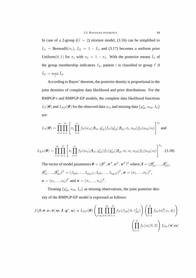
3.3. BAYESIAN INFERENCE 84
In case of a 2-group (G = 2) mixture model, (3.16) can be simplified to
Ii1 ∼ Bernoulli(π1), Ii2 = 1 − Ii1 and (3.17) becomes a uniform prior
Uniform(0, 1) for π1 with π2 = 1 − π1. With the posterior means Iil of
the group membership indicators Iil, patient i is classified to group l′ if
Iil′ = maxlIil.
According to Bayes’ theorem, the posterior density is proportional to the
joint densities of complete data likelihood and prior distributions. For the
RMPGP-t and RMPGP-EP models, the complete data likelihood functions
LT (θ) and LEP (θ) for the observed data wit and missing data {y∗itl, uitl, Iil}
are:
LT (θ) =m∏
i=1
G∏
l=1
[πl
ni∏
t=1
fP (wit|βal, y∗itl)fN(y∗itl|βµl, σl, uitl)fG(uitl| νl)
]Iil
and
LEP (θ) =m∏
i=1
G∏
l=1
[πl
ni∏
t=1
fP (wit|βal, y∗itl)fU(y∗itl|βµl, σl, νl, uitl)fG(uitl| νl)
]Iil
. (3.18)
The vector of model parameters θ = (βT ,σT ,νT ,πT )T where β = (βTµ1, ...,β
TµG,
βTa1, ...,β
TaG)T = (βµ01, ..., βµqµG, βa01, ..., βaqaG)T , σ = (σ1, ..., σG)T ,
ν = (ν1, ..., νG)T and π = (π1, ..., πG)T .
Treating {y∗itl, uitl, Iil} as missing observations, the joint posterior den-
sity of the RMPGP-EP model is expressed as follows:
f(β,σ,ν,π|w, I,y∗,u) ∝ LEP (θ)
(∏
j=µ,a
qj∏
k=0
G∏
l=1
fN(βjkl| 0, τ 2jkl)
)(G∏
l=1
fIG(σ2l | cl, dl)
)
(G∏
l=1
fU(νl| 0, 2))fDir(π|α)

3.3. BAYESIAN INFERENCE 85
where w = (w11, w12, ..., wmnm)T , I = (I11, I12, ..., ImG)T , y∗ = (y∗111, y
∗121, ..., y
∗mnmG)T
and u = (u111, u121, ..., umnmG)T . The complete data likelihood LEP (θ)
of the RMPGP-EP model is given by (3.18) and the priors are given by
(3.13)-(3.17). In Gibbs sampling, the unknown parameters are simulated it-
eratively from their univariate conditional posterior distributions which are
proportional to the joint posterior density of complete data likelihood and
prior densities.
The univariate full conditional posterior densities for each of the un-
known model parameters in θ and missing observations in {y∗,u, I} are
given by:
f(βµkl|w, I,y∗,u,β−,σ,ν,π) ∝ exp
(−β2
µkl
2τ 2µkl
)restricted to
βµkl ∈[z−1
µkit maxi, t
(y∗itl − σluνl/2itl −
∑
κ6=k
βµκlzµκit), z−1µkit min
i, t(y∗itl + σlu
νl/2itl −
∑
κ6=k
βµκlzµκit)
],
if zµkit 6= 0
f(βakl|w, I,y∗,u,β−,σ,ν,π) ∝ exp
{−
m∑
i=1
Iil
ni∑
t=1
[ey∗
itl
at−1itl
+ βaklzakit(t− 1)wit
]− β2
akl
2τ 2akl
}
f(y∗itl|w, I,y∗−,u,β,σ,ν,π) ∝ exp
(− ey∗
itl
at−1itl
+ y∗itlwit
)
restricted to y∗itl ∈ (µ∗itl − σlu
νl/2itl , µ
∗itl + σlu
νl/2itl )
f(σ2l |w, I,y∗,u,β,σ−,ν,π) ∝ σ
−(mP
i=1niIil+2cl+2)
l exp
(− dl
σ2l
)
restricted to σ2l > max
i, t
[(y∗itl − µ∗
itl)2
uνl
itl
]
f(uitl|w, I,y∗,u−,β,σ,ν,π) ∝ exp(−uitl
2
)restricted to uitl >
(y∗itl − µ∗
itl
σl
)2/νl

3.3. BAYESIAN INFERENCE 86
f(νl|w, I,y∗,u,β,σ,ν−,π) ∝[Γ(νl
2+ 1)
2νl2
]− mPi=1
niIil
restricted to νl > maxi,t
ln(
y∗
itl−µ∗
itl
σl
)2
ln uitl
f(I i|w, I−,y∗,u,β,σ,ν,π) ∝G∏
l=1
πl
ni∏t=1
exp
„− e
y∗itl
at−1itl
−uitl2
«„ey∗itl
at−1itl
«wit
σlΓ(νl2
+1)2νl2
G∑l′=1
πl′
ni∏t=1
exp
− e
y∗itl′
at−1itl′
−u
itl′
2
! ey∗itl′
at−1itl′
!wit
σl′Γ(νl′
2+1)2
νl′2
Iil
=G∏
i=1
π′ Iil
il = Multinomial(1, π′i1, . . . , π
′iG)
f(πl|w, I,y∗,u,β,σ,ν,π−) ∝ π
mPi=1
Iil+αl−1
l
where β−,y∗−,u−,σ−,ν−,π− and I− and are vectors of β,y∗,u,σ,ν,π
and I excluding βjkl, y∗itl, uitl, σl, νl, πl and I i = (Ii1, . . . , IiG)T respec-
tively. The MCMC algorithms can be derived for the RMPGP-t model in
a similar way. Nevertheless, the MCMC algorithms are implemented using
the user-friendly software WinBUGS where the sampling scheme based on
the conditional posterior densities is outlined in this Section and the Gibbs
sampling procedures are described in Section 1.4.3.
3.3.3. Model selection criterion. For the simulation experiment in Sec-
tion 3.4 and data analysis in Section 3.5, we adopt the deviance information
criterion (DIC), originated by Spiegelhalter et al. (2002), as the model se-
lection criterion. Deviance information criterion (DIC) is a sum of the
posterior mean deviance D(θ) measuring the model fit and the effective

3.3. BAYESIAN INFERENCE 87
dimension pD which accounts for the model complexity. For the RMPGP
model, the DIC is defined as
DIC = D(θ) + pD
= − 4
M
M∑
j=1
m∑
i=1
G∑
l=1
I′(j)il
[lnπ
(j)l +
ni∑
t=1
ln{fP (wit| y∗(j)itl ,β
(j)al )fD(y
∗(j)itl |β(j)
µl , σ(j)l , ν
(j)l )}]
+2m∑
i=1
G∑
l=1
I ′il
[ln πl +
ni∑
t=1
ln{fP (wit| y∗itl, βal)fD(y∗itl| βµl, σl, νl)
}]
(3.19)
where M is the number of realizations in the MCMC sampling algorithms,
fD(·), D = T or EP are densities given by (3.4) and (3.6) for the RMPGP-
t and RMPGP-EP models respectively, βal = (βa0l, ..., βaqal)T , βµl =
(βµ0l, ..., βµqµl)T , and θ(j) and θ represent the jth posterior sample and pos-
terior mean of parameter θ respectively,
I′(j)il =
π(j)l
ni∏t=1
{fP (wit| y∗(j)itl ,β
(j)al )fD(y
∗(j)itl |β(j)
µl , σ(j)l , ν
(j)l )}
G∑l′=1
π(j)l′
ni∏t=1
{fP (wit| y∗(j)itl′ ,β
(j)al′ )fD(y
∗(j)itl′ |β
(j)µl′ , σ
(j)l′ , ν
(j)l′ )} ,
and I ′il is defined in a similar way by replacing y∗(j)itl and θ(j) with y∗itl and
θ. The rule of thumb is that the smaller the DIC, the better is the model.
3.3.4. Test for serial correlation. Parameter interpretation and predic-
tion are made based on the best model. After investigating the trend, cluster
and covariate effects, the remaining unexplained variation is used to test for
serial correlation. In order to calculate the Pearson’s residuals, the marginal
mean and variance of the outcome Wit are needed. Denote the conditional
mean and variance on the group being analyzed by El(Wit) and V arl(Wit)
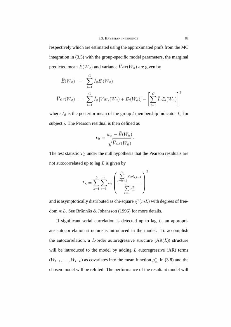
3.3. BAYESIAN INFERENCE 88
respectively which are estimated using the approximated pmfs from the MC
integration in (3.5) with the group-specific model parameters, the marginal
predicted mean E(Wit) and variance V ar(Wit) are given by
E(Wit) =G∑
l=1
IilEl(Wit)
V ar(Wit) =G∑
l=1
Iil [V arl(Wit) + El(Wit)] −[
G∑
l=1
IilEl(Wit)
]2
where Iil is the posterior mean of the group l membership indicator Iil for
subject i. The Pearson residual is then defined as
εit =wit − E(Wit)√V ar(Wit)
.
The test statistic TL under the null hypothesis that the Pearson residuals are
not autocorrelated up to lag L is given by
TL =L∑
k=1
m∑
i=1
ni
ni∑t=k+1
εitεi,t−k
ni∑t=1
ε2it
2
and is asymptotically distributed as chi-square χ2(mL) with degrees of free-
dom mL. See Brannas & Johansson (1996) for more details.
If significant serial correlation is detected up to lag L, an appropri-
ate autocorrelation structure is introduced in the model. To accomplish
the autocorrelation, a L-order autoregressive structure (AR(L)) structure
will be introduced to the model by adding L autoregressive (AR) terms
(Wt−1, . . . ,Wt−L) as covariates into the mean function µ∗itl in (3.8) and the
chosen model will be refitted. The performance of the resultant model will

3.4. SIMULATION STUDY 89
be evaluated based on the significance of the model parameters in the AR
structure and the model selection criterion DIC .
3.4. Simulation study
To investigate the properties of the RPGP-t and RPGP-EP models, we
conducted a simulation study in which h = 100 data sets are simulated from
each of the RPGP models based on a set of true parameters. For simplicity,
we set G = 1, qµ = qa = 1 and each data set contains m = 80 time series
of length ni = 8 from m0 = 40 subjects in the control group (b = 0) and
another m1 = 40 subjects in the treatment group (b = 1) with zµ1it = b
in the mean function in (3.2). The degrees of freedom ν is set to include
heavy (ν = 2.5) and light (ν = 50) tails for Student’s t-distribution and
platykurtic (ν = 0.1) and leptokurtic (ν = 1.8) shapes for EP distribution.
The parameter βa1 in the ratio function in (3.3) with za1it = t is also set
to include different trend patterns by varying the sign and magnitude of the
true value.
Afterwards both models are fitted to each data set using the Bayesian ap-
proach implemented by WinBUGS and R2WinBUGSwhich are described in
Section 1.4.3. For the hyperparameters in the prior distributions (dropping
the subscript ‘l’ sinceG = 1), we assign τ 2jk = 1000 in (3.13), c = d = 0.01
in (3.14) and e = 150 in (3.15). The parameter estimate θ is given by the
average of h = 100 posterior medians θj . To examine the precision of the
MCMC algorithms, the standard deviation (SD) of θj over h = 100 sim-
ulated data sets for each parameter θ is reported. In addition, to assess the

3.4. SIMULATION STUDY 90
accuracy of parameter estimates when the data set is simulated and fitted
to the same model, we calculate the mean squared error (MSE) for each
parameter θ which is defined as:
MSE =1
h
h∑
j=1
(θj − θ)2.
For model selection, the averageDIC and average squared error (ASE)
proposed by Wegman (1972) are used to assess the quality of the density
estimator on the true pmf. Denote the true pmf of the RMPGP model by
fbt(w) at time t with covariate b, the ASE is used to compare the perfor-
mance of the two models fitted to the same simulated data set and is defined
as
ASE =∑
b=0,1
ψb
ni∑
t=1
h∑
j=1
∞∑
w=0
{f
(j)bt (w) − fbt(w)
}2
where f (j)bt (w) is the pmf estimator of (3.1) using MC integration described
in (3.5) for counts w in the jth simulated set at time t with treatment effect b
and ψb =mb
mis the weight associated with the control (b = 0) or treatment
group (b = 1). Clearly, the smaller the ASE, the closer is the estimated
pmf to the true one and thus the better is the model performance.
Table 3.3 in Appendix 3.2 summarizes the results of the four sets of sim-
ulation experiments with the first two data sets simulated from the RPGP-t
model and the next two simulated from the RPGP-EP model. In general, the
MCMC algorithms give unbiased and precise estimates as both MSE and
SD of most parameters are reasonably small. Moreover, the values of the
shape parameter ν of the two models match with each other in terms of the
3.5. REAL DATA ANALYSIS 91
tailedness. For example, the small ν = 5.286 in the Student’s t-distribution
in data set 1 agrees with ν = 1.8234 which is close to 2 in the EP distri-
bution. However, it is noticed that ν of the RPGP-t model has relatively
lower precision and higher bias reflecting the higher level of difficulty in
estimating the tailedness of the heavy-tailed Student’s t-distribution.
==================================
Table 3.3 about here
==================================
In model comparison, although the RPGP-t model has a slightly smaller
ASE (0.04504 versus 0.04817 averaged over the four simulated data sets),
the RPGP-EP model outperforms the RPGP-t model with smaller DIC
(1968.4 versus 1979.48). All in all, these simulation experiments show that
the performance of the MCMC algorithms for the two models is satisfactory
and the estimated pmfs f (j)bt (w) approximate the true pmfs fbt(w) reason-
ably well. While EP distribution can be platykurtic or leptokurtic with a
kink and Student’s t-distribution can give a very heavy tail when the outly-
ing effect is tremendous, the two RPGP models are suitable under different
circumstances.
3.5. Real data analysis
3.5.1. Data and model fitting. We illustrate the usefulness of our pro-
posed models through the epilepsy data which can be found in Thall & Vail
(1990) and given in Appendix 3.1. The data were collected from a clinical
trial of 59 epileptics by Leppik et al. (1985). In the randomized controlled

3.5. REAL DATA ANALYSIS 92
trial, m = 59 patients suffering from simple or complex partial seizures
were assigned to either the antiepileptic drug progabide (zµ1i = 1) or the
placebo (zµ1i = 0) with no intrinsic therapeutic value. The seizure counts
were recorded at a two-week interval for an eight-week period (ni = 4)
with no dropout or missing cases. As shown in Table 3.4 in Appendix 3.2,
the seizure counts exhibit a prominent extra-Poisson variation with large
variance to mean ratios at all time t due to some outlying observations
as displayed in Figures 3.4(a) and 3.4(b) in Appendix 3.3. To assess the
overdispersion in the data, we fitted a simple Poisson regression model us-
ing a mean link function ηit = exp(β0 + β1zµ1i + β2t) and a simplified
PGP model in Wan (2006) using a mean function µit = exp(βµ0 + βµ1zµ1i)
and a ratio function ait = exp(βa0 + βa1t). The mean and variance under
both models are equivalent (indicated by ‘*’ in Table 3.4) and are given by
ηit andµit
at−1it
respectively. Obviously, neither of the two simple models, as
restricted by their equidispersed property, can capture the overdispersion.
Besides, the higher mean seizure counts of the placebo group indicate that
‘treatment group’ is a feasible covariate. Moreover, the gradually decreas-
ing seizure counts over time for both placebo and progabide groups suggest
that time t maybe a possible time-evolving covariate. In addition, popu-
lation heterogeneity in terms of trend pattern and count level is detected
intuitively. In consideration of these and the clinical interest of examining
the trend patterns, we adopt the RMPGP models to analyze the epilepsy
data.

3.5. REAL DATA ANALYSIS 93
====================================
Figures 3.4(a) and 3.4(b) and Table 3.4 about here
====================================
Referring to the MCMC algorithms detailed in Section 3.3.2, our prior
specifications are mostly non-informative except for νl in the RMPGP-t
model. In both RMPGP models, we assign τ 2jkl = 1000 in (3.13), cl =
dl = 0.001 in (3.14) and αl = 1/G in (3.17) for a G-group (G ≥ 2) model.
For νl in the RMPGP-t model, we take el = 20 since there is a high degree
of overdispersion in the seizure counts. After implementing the MCMC
algorithms in WinBUGS, the posterior sample means are adopted as param-
eter estimates since the posterior densities of most model parameters are
highly symmetric such that the posterior sample mean is close to the poste-
rior sample median.
We first fitted a simple RPGP model with treatment group (zµ1it = 0, 1)
as the covariate in the mean function µitl in (3.8) and two-week interval
(za1it = t = 1, 2, 3, 4) as the time-evolving effect in the ratio function
aitl in (3.9). The insignificant βµ1’s in both RPGP models indicate that
the progabide treatment effect is insignificant (95% CIs for βµ1 in RPGP-t
model and RPGP-EP model include zero). However, within the treatment
group, it is explicit that some of these patients have abnormally high seizure
counts. Simply fitting a simple RPGP model may fail to allow for the cluster
effect among patients receiving the same treatment. We therefore fitted
the 2-group and 3-group RMPGP models using both Student’s t- and EP

3.5. REAL DATA ANALYSIS 94
distributions but the results indicate that one of the groups in the 3-group
RMPGP models degenerated and hence the models are discarded. Table 3.5
in Appendix 3.2 summarizes the parameter estimates, standard errors (SE)
and model selection criterion DIC of the 1-group and 2-group RMPGP
models.
==================================
Table 3.5 about here
==================================
3.5.2. Results. Not surprisingly, both RMPGP models give parallel re-
sults as they share some common model properties except the shape of the
distribution of y∗itl. In the RMPGP-t model, two distinct groups of patients
are identified with the first group of patients having generally higher seizure
counts and is named as the high-level group (l = 1). Within this group, 54%
of the patients are receiving progabide and they have lower seizure counts in
general (βµ11 < 0) than those receiving placebo. However, the difference is
insignificant since the 95% CI for βµ11 is [−0.7197, 0.0426] which includes
zero. Whereas in the low-level (l = 2) group, 49% of the patients belong
to the progabide group and again they generally have less epileptic seizures
during the studying period (βµ12 < 0, 95% CI:[−0.5992,−0.0921]). More-
over, the ratio function ait1 in (3.9) reveals that there is a slightly decreasing
trend in the seizure counts in the high-level group while ait2 indicates that
no obvious trend is detected in the low-level group. In addition, comparing
with the low-level group, the relatively smaller ν1 shows that the high-level

3.5. REAL DATA ANALYSIS 95
group has a higher degree of overdispersion in the seizure counts due to
the existence of some abnormally large observations as revealed in Figures
3.4(a) and 3.4(b).
As expected, the RMPGP-EP model gives consistent results in terms
of trend pattern and treatment effect. Moreover, the group membership
of the patients has a close affinity with that of RMPGP-t model and two
diverse groups, high-level and low-level groups, are recognized as well. But
for the high-level group, despite the comparable mean level, the difference
between the two treatment effects becomes significant (95% CI for βµ11:
[−0.5992,−0.0921]). Furthermore, the ratio function ait1 shows that the
seizure count increases until the second 2-week interval (t = 2) before it
drops in the next two 2-week intervals. Consistently, the estimate ν1 = 1.49
(leptokurtic shape in the EP distribution) agrees with the small ν1 = 7.21
(heavier-than-normal tail in the Student’s t-distribution) in the RMPGP-t
model indicating that the distribution of the seizure counts in the high-level
group has a heavier tail to account for the higher degree of overdispersion.
On the other hand, the smaller ν2 = 0.24 (platykurtic in the EP distribution)
indicates the model distribution is more uniform in the low-level group.
For model selection, the smallerDIC given by (3.19) as shown in Table
3.5 for the RMPGP-EP model manifests its better model fit on the epilep-
tic seizure counts after accounting for the model complexity. A plausible
explanation is that the EP distribution has a more flexible tail behaviour
and thus provides a better fit to the data. To further investigate this, their

3.5. REAL DATA ANALYSIS 96
observed and fitted pmfs for the low-level group are illustrated in Figures
3.5(a) to 3.5(d) in Appendix 3.3 at different time points in Appendix 3.3.
The observed pmf ftl(w) for group l at time t is generally given by
ftl(w) =∑
b=0,1
ψb
m∑i=1
IilI(Wit = w)I(zµ1i = b)
∞∑w′=0
m∑i=1
IilI(Wit = w′)I(zµ1i = b)
, w = 0, 1, 2, . . . (3.20)
where I(Wit = w) is an indicator which returns 1 whenWit = w for patient
i at time t in group l and 0 otherwise, I(zµ1i = b) indicates the treatment
group b of patient i, Iil is the posterior mean of the group membership indi-
cator and ψb is the weight associated with the placebo (b = 0) or progabide
group (b = 1). On the other hand, the fitted pmf ftl(w) is obtained similarly
by
ftl(w) =∑
b=0,1
ψbfbtl(w), w = 0, 1, 2, . . .
where fbtl(w) is approximated by MC integration in (3.5) based on the pa-
rameter estimates θl = (βTµl,β
Tal, σl, νl)
T . According to Figures 3.5(a) to
3.5(d), both models imitate the observed pmfs reasonably well. However,
the predicted trend in the low-level group cannot accommodate the upsurge
in the observation w = 4 at t = 2 resulting in a discrepancy between the
observed and fitted pmfs as shown in Figure 3.5(b). It is not surprising to
find that the two RMPGP models give similar pmfs as both have the ca-
pability of modelling highly overdispersed data. Nevertheless, despite the
affinity, the slightly heavier tail in the distribution of the RMPGP-EP model
possibly gives rise to the lower DIC.

3.5. REAL DATA ANALYSIS 97
In the best model (RMPGP-EP model), extra variation is added to the
mean of the Poisson distribution through the mixing distribution. Therefore,
the variances of the estimated pmf ftl(w) of each treatment group given by
(2.19) and the overall variances which comprises the variance of expectation
and the expectation of variance conditional on the mixture group given by
(2.18) show a dramatic improvement. For example, when t = 1, the overall
variance of the RMPGP-EP model (137.23) is closer to the observed vari-
ance (220.08) than that of the PGP model (8.8729). These two variances
are reported in Table 3.4 in Appendix 3.2.
==================================
Figures 3.5(a) to 3.5(d) about here
==================================
Advantageously, implementing the model using Bayesian approach en-
ables us to study the latent stochastic process {y∗itl} and the mixing pa-
rameters uitl. These unobserved parameters can be output by using the
Convergence Diagnostic and Output Analysis (CODA) software in WinBUGS.
The CODA is a menu-driven set of S-Plus functions which produces an
output file storing the posterior samples of all model parameters with their
corresponding iteration numbers. For the RMPGP-EP model, to examine
the density of the unobserved y∗itl which are simulated from an EP distribu-
tion with location parameter µ∗itl, scale parameter σl and shape parameter
νl, we compare the densities of the posterior samples of y∗itl with the normal
3.5. REAL DATA ANALYSIS 98
distribution which has the same mean and standard deviation as the pos-
terior samples and the EP distribution also with same mean and standard
deviation and a shape parameter νl. Four selected y∗itl from each mixture
group l and treatment group zµ1i = b = 0, 1 are illustrated in Figure 3.6 in
Appendix 3.3. Obviously, the y∗it1’s have a leptokurtic shape whereas y∗it2’s
appear to be more uniform than the normal distribution. These agree with
the results in Table 3.5 that the shape parameter of the high-level group is
larger than that of the low-level group (ν1 > ν2) and explain how the EP
distribution can downweigh the outlying effect.
==================================
Figure 3.6 about here
==================================
Furthermore, the outlier diagnosis is performed using the mixing pa-
rameter estimates uitl in the RMPGP-EP model. An unusually large uitl in-
dicates that the observation wit is possibly an outlier under group l. For fair
comparison, we calculate the standardized observations w′itl =
|wit − witl|σwitl
for patient i where witl and σwitlare respectively the mean and standard de-
viation of the observed pmf ftl(w) in (3.20) at time t under group l. Both
mixing parameters uitl and standardized seizure counts w′itl are sorted by
groups (l = 1, 2) for better visualization and are then plotted in Figure 3.7
in Appendix 3.3.
3.5. REAL DATA ANALYSIS 99
==================================
Figure 3.7 about here
==================================
Clearly, all the top 10 (5%) outlying counts with the first 10 largest uitl
locate in the high-level group (l = 1) due to the presence of some extreme
observations. They are highlighted in Figure 3.7 with the corresponding
rank and observation wit in parentheses. Not surprisingly, the correlation
between uit1 and w′it1 is high (ruw = 0.9731) which signifies the appro-
priateness of using the mixing parameters in outlier diagnosis. While the
outlying effect is not substantial in the low-level group (l = 2), uit2 appears
to be relatively smaller.
The top four outlying values come from the same patient with ID 49
who has abnormally high seizure counts at each 2-week interval. Besides,
two large observations are identified from patients with ID 8 (w8,1 = 40)
and 25 (w25,3 = 76) in Figure 3.7. In spite of large observation, four small
seizure counts are also classified as outlier from patients with ID 10, 24,
39 and 56. Knowing which patients are associated with abnormal seizure
counts, specialists can pay more attention to their abnormalities and alter-
native treatments may be considered accordingly. Besides the detection of
outliers using the mixing parameters, the RMPGP-EP model also down-
weighs the outlying effect and thus the general trend pattern is not distorted
by the extreme observations.
3.6. DISCUSSION 100
Last but not least, we tested for the serial correlation in the best model
by using the procedures described in Section 3.3.4. Starting from some
lower lags, the large p-values of the chi-square tests for autocorrelation up
to lag 1 (0.837) and lag 2 (0.999) affirm that there is no evidence of the
presence of autocorrelation up to lag 2. Hence the tests for higher lags are
not considered and the RMPGP-EP model is validated.
3.6. Discussion
In this Chapter, we extend the Poisson geometric process (PGP) model
in Wan (2006) to allow for extra-Poisson variation when extreme observa-
tions appear in the data. Ignoring the outlying effects may lead to over-
estimated mean and variance resulting in invalid interpretation and predic-
tion. As remedies, two methods are suggested to account for overdispersion
which include adopting a heavy-tailed distribution and incorporating mix-
ture effect. The latter can handle cluster effect in the data and overdispersion
arisen from that may also be captured.
As a new direction to account for extreme observations leading to overdis-
persion and population heterogeneity, we apply the heavy-tailed distribu-
tions in the modelling of longitudinal count data and pioneer the robust
Poisson geometric process (RPGP) model. This model allows the mean Xit
of the Poisson distribution to follow a GP and the logarithm of the underly-
ing stochastic process {Yit = at−1it Xit} follows a heavy-tailed distribution.
The resultant model is called the RPGP model. By varying a set of model
parameters, the moments of the RPGP models are reported in Tables 3.1 and

3.6. DISCUSSION 101
3.2 in Appendix 3.2 and their pmfs are revealed in Figures 3.1 and 3.2 in
Appendix 3.3. Although the marginal pmfs do not have closed-form, Monte
Carlo (MC) integration in (3.5) can be used to approximate the pmfs, and
hence the mean as well as the variance. Tables 3.1 and 3.2 in Appendix
3.2 show that the model can accommodate both equidispersed and overdis-
persed data with varying kurtoses.
The RPGP models and the RMPGP models which can allow for clus-
ter effects are implemented using a Bayesian approach. Expressing the
heavy-tailed distribution in a scale mixtures form facilitates the model im-
plementation using MCMC algorithms and the mixing parameter enables
us to perform outlier diagnosis as shown in the real data analysis. Here,
the Student’s t-distribution in scale mixtures of normals (SMN) and expo-
nential power (EP) distribution in scale mixtures of uniforms (SMU) are
adopted. Regarding serial correlation, a test is described in Section 3.3.4
for detecting an up-to-lag-L autocorrelation and some lagged observations
can be easily incorporated into the mean function µ∗itl in (3.8) as covari-
ates if needed. The resultant models can be efficiently implemented via the
user-friendly software, WinBUGS.
In addition, the simulation study shows that the performances of the two
RPGP models are comparable and satisfactory. In the case of data with a
very long tail, the RMPGP-t model seems to fit better since the tail of the
Student’s t-distribution is much heavier than that of the normal distribution.
On the other hand, the RMPGP-EP model gives a better fit in the analysis

3.6. DISCUSSION 102
of epilepsy data with more diverse degrees of overdispersion across mixture
groups as EP distribution has a more flexible shape which can be either
leptokurtic or platykurtic.
Lastly, one pitfall of the RMPGP model is that taking log-transformation
of the latent stochastic process {Yit} inevitably causes those data associated
with close-to-zero means being identified as outliers. Hence when zero
is dominant in the data, the proposed RMPGP models can be extended to
include a zero-altered component as in the zero-altered MPGP model intro-
duced in Chapter 2.

3.6. DISCUSSION 103
Appendix 3.1
Successive two-week seizure counts Wit for 59 epilepticsin two treatment groups (0=placebo, 1=progabide)
patient wi1 wi2 wi3 wi4 treatment
1 5 3 3 3 02 3 5 3 3 03 2 4 0 5 04 4 4 1 4 05 7 18 9 21 06 5 2 8 7 07 6 4 0 2 08 40 20 23 12 09 5 6 6 5 0
10 14 13 6 0 011 26 12 6 22 012 12 6 8 5 013 4 4 6 2 014 7 9 12 14 015 16 24 10 9 016 11 0 0 5 017 0 0 3 3 018 37 29 28 29 019 3 5 2 5 020 3 0 6 7 021 3 4 3 4 022 3 4 3 4 023 2 3 3 5 024 8 12 2 8 025 18 24 76 25 026 2 1 2 1 027 3 1 4 2 028 13 15 13 12 029 11 14 9 8 130 8 7 9 4 131 0 4 3 0 132 3 6 1 3 133 2 6 7 4 134 4 3 1 3 135 22 17 19 16 136 5 4 7 4 137 2 4 0 4 138 3 7 7 7 139 4 18 2 5 140 2 1 1 0 141 0 2 4 0 142 5 4 0 3 143 11 14 25 15 144 10 5 3 8 145 19 7 6 7 146 1 1 2 4 147 6 10 8 8 148 2 1 0 0 149 102 65 72 63 150 4 3 2 4 151 8 6 5 7 152 1 3 1 5 153 18 11 28 13 154 6 3 4 0 155 3 5 4 3 156 1 23 19 8 157 2 3 0 1 158 0 0 0 0 159 1 4 3 2 1

3.6. DISCUSSION 104
Appendix 3.2
Tables
Table 3.1: Moments of marginal pmfs for RPGP-t model under a set of
floating parameters with fixed values of ν = 10, σ = 0.5, βµ0 = 3, βµ1 =
−0.2, βa0 = 0.5, βa1 = −0.1
floating floatingparameter mean variance kurtosis parameter mean variance kurtosis
ν = 1 15.082 152.634 1.0017 σ = 0.1 12.279 14.110 0.1209
ν = 2 14.381 110.855 1.0036 σ = 0.5 14.041 81.182 0.5579
ν = 5 14.616 103.899 0.6568 σ = 1.0 16.143 230.454 0.9817
ν = 50 13.985 69.826 0.3827 σ = 2.0 15.511 349.030 0.9832
βµ0 = 1.0 1.057 1.643 0.0411 βa0 = −0.5 34.452 262.605 0.9605
βµ0 = 2.0 2.891 6.827 0.2277 βa0 = −0.01 23.015 175.040 0.8652
βµ0 = 3.0 7.832 32.123 0.7399 βa0 = 0.5 14.460 95.392 0.7662
βµ0 = 4.0 20.814 153.217 1.1929 βa0 = 1.5 5.344 16.972 0.2819
Table 3.2: Moments of marginal pmfs for RPGP-EP model under a set of
floating parameters with fixed values of ν = 1, σ = 0.5, βµ0 = 3, βµ1 =
−0.5, βa0 = 0.5, βa1 = −0.1
floating floatingparameter mean variance kurtosis parameter mean variance kurtosis
ν = 0.1 9.379 16.987 0.0925 σ = 0.1 9.048 9.871 0.0782
ν = 0.5 9.629 20.468 0.1312 σ = 0.5 10.331 42.865 0.2938
ν = 1.0 10.174 39.574 0.3281 σ = 1.0 13.891 197.640 0.9747
ν = 2.0 12.592 192.360 0.9835 σ = 2.0 14.627 327.645 0.9840
βµ0 = 1.0 1.382 1.956 0.0388 βa0 = −0.5 26.592 198.533 0.9605
βµ0 = 2.0 3.771 7.695 0.0982 βa0 = −0.01 16.845 104.392 0.8652
βµ0 = 3.0 10.386 46.856 0.3061 βa0 = 0.5 10.216 46.338 0.7662
βµ0 = 4.0 27.046 199.776 0.7261 βa0 = 1.5 3.788 10.512 0.2819
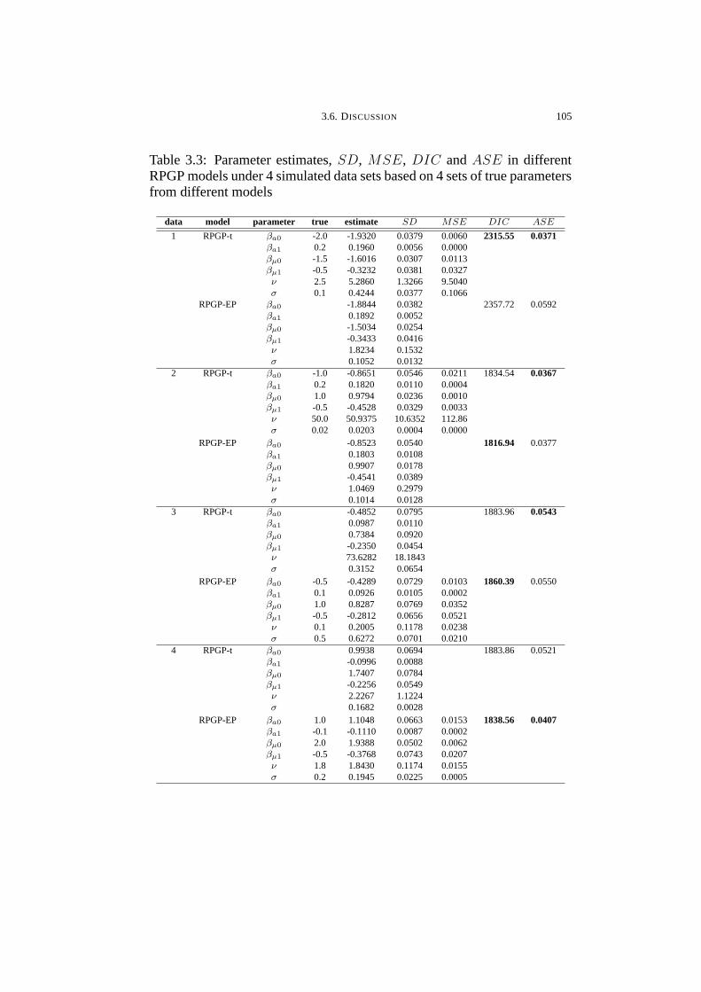
3.6. DISCUSSION 105
Table 3.3: Parameter estimates, SD, MSE, DIC and ASE in differentRPGP models under 4 simulated data sets based on 4 sets of true parametersfrom different models
data model parameter true estimate SD MSE DIC ASE
1 RPGP-t βa0 -2.0 -1.9320 0.0379 0.0060 2315.55 0.0371βa1 0.2 0.1960 0.0056 0.0000βµ0 -1.5 -1.6016 0.0307 0.0113βµ1 -0.5 -0.3232 0.0381 0.0327ν 2.5 5.2860 1.3266 9.5040σ 0.1 0.4244 0.0377 0.1066
RPGP-EP βa0 -1.8844 0.0382 2357.72 0.0592βa1 0.1892 0.0052βµ0 -1.5034 0.0254βµ1 -0.3433 0.0416ν 1.8234 0.1532σ 0.1052 0.0132
2 RPGP-t βa0 -1.0 -0.8651 0.0546 0.0211 1834.54 0.0367βa1 0.2 0.1820 0.0110 0.0004βµ0 1.0 0.9794 0.0236 0.0010βµ1 -0.5 -0.4528 0.0329 0.0033ν 50.0 50.9375 10.6352 112.86σ 0.02 0.0203 0.0004 0.0000
RPGP-EP βa0 -0.8523 0.0540 1816.94 0.0377βa1 0.1803 0.0108βµ0 0.9907 0.0178βµ1 -0.4541 0.0389ν 1.0469 0.2979σ 0.1014 0.0128
3 RPGP-t βa0 -0.4852 0.0795 1883.96 0.0543βa1 0.0987 0.0110βµ0 0.7384 0.0920βµ1 -0.2350 0.0454ν 73.6282 18.1843σ 0.3152 0.0654
RPGP-EP βa0 -0.5 -0.4289 0.0729 0.0103 1860.39 0.0550βa1 0.1 0.0926 0.0105 0.0002βµ0 1.0 0.8287 0.0769 0.0352βµ1 -0.5 -0.2812 0.0656 0.0521ν 0.1 0.2005 0.1178 0.0238σ 0.5 0.6272 0.0701 0.0210
4 RPGP-t βa0 0.9938 0.0694 1883.86 0.0521βa1 -0.0996 0.0088βµ0 1.7407 0.0784βµ1 -0.2256 0.0549ν 2.2267 1.1224σ 0.1682 0.0028
RPGP-EP βa0 1.0 1.1048 0.0663 0.0153 1838.56 0.0407βa1 -0.1 -0.1110 0.0087 0.0002βµ0 2.0 1.9388 0.0502 0.0062βµ1 -0.5 -0.3768 0.0743 0.0207ν 1.8 1.8430 0.1174 0.0155σ 0.2 0.1945 0.0225 0.0005

3.6. DISCUSSION 106
Table 3.4: Mean and variance for the observed epilepsy data and of two
simple fitted and RMPGP-EP models
time averagemodel t = 1 t = 2 t = 3 t = 4 over time
placebomean observed 9.3571 8.2857 8.7857 8.0000 8.6071
Poisson* 9.3658 8.8385 8.3410 7.8714 8.6042
PGP* 9.2073 8.9707 8.4645 7.7348 8.5943
RMPGP-EP 10.047 10.4001 9.9565 8.7905 9.7984
variance observed 102.76 66.656 215.29 57.926 107.93
RMPGP-EP 187.19 214.02 198.25 141.92 185.34
progabidemean observed 8.5806 8.4194 8.1290 6.7419 7.9677
Poisson* 8.6700 8.1819 7.7214 7.2867 7.9557
PGP* 8.5212 8.3023 7.8337 7.1584 7.9539
RMPGP-EP 6.8235 7.2885 6.9278 5.9980 6.7595
variance observed 332.72 140.65 193.05 126.66 193.97
RMPGP-EP 92.114 124.37 107.44 77.371 100.32
overallmean observed 8.9492 8.3559 8.4407 7.3390 8.2712
Poisson* 8.9940 8.4920 8.0179 7.5704 8.2686
PGP* 8.8729 8.6469 8.1573 7.4495 8.2816
RMPGP-EP 8.3531 8.7652 8.3652 7.3233 8.2017
variance observed 220.08 103.78 200.18 92.883 152.61
RMPGP-EP 137.23 166.92 150.54 108.00 140.67
* indicates mean and variance are equivalent.
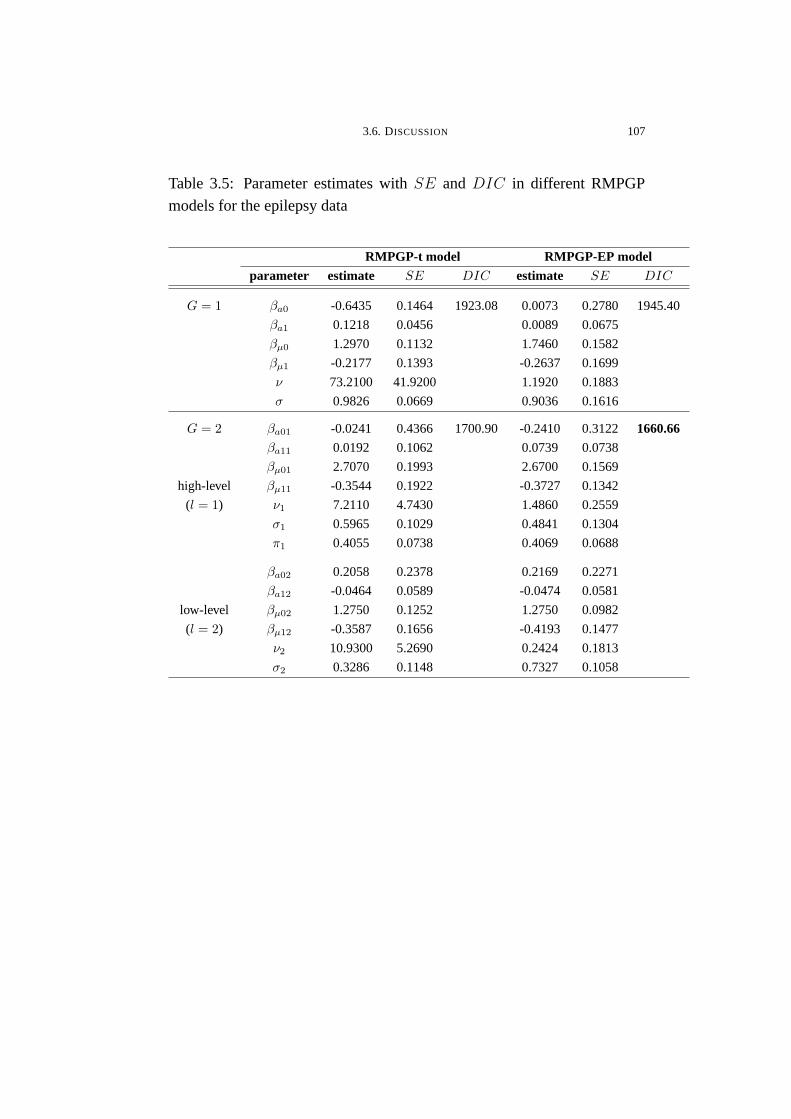
3.6. DISCUSSION 107
Table 3.5: Parameter estimates with SE and DIC in different RMPGP
models for the epilepsy data
RMPGP-t model RMPGP-EP modelparameter estimate SE DIC estimate SE DIC
G = 1 βa0 -0.6435 0.1464 1923.08 0.0073 0.2780 1945.40
βa1 0.1218 0.0456 0.0089 0.0675
βµ0 1.2970 0.1132 1.7460 0.1582
βµ1 -0.2177 0.1393 -0.2637 0.1699
ν 73.2100 41.9200 1.1920 0.1883
σ 0.9826 0.0669 0.9036 0.1616
G = 2 βa01 -0.0241 0.4366 1700.90 -0.2410 0.3122 1660.66βa11 0.0192 0.1062 0.0739 0.0738
βµ01 2.7070 0.1993 2.6700 0.1569
high-level βµ11 -0.3544 0.1922 -0.3727 0.1342
(l = 1) ν1 7.2110 4.7430 1.4860 0.2559
σ1 0.5965 0.1029 0.4841 0.1304
π1 0.4055 0.0738 0.4069 0.0688
βa02 0.2058 0.2378 0.2169 0.2271
βa12 -0.0464 0.0589 -0.0474 0.0581
low-level βµ02 1.2750 0.1252 1.2750 0.0982
(l = 2) βµ12 -0.3587 0.1656 -0.4193 0.1477
ν2 10.9300 5.2690 0.2424 0.1813
σ2 0.3286 0.1148 0.7327 0.1058
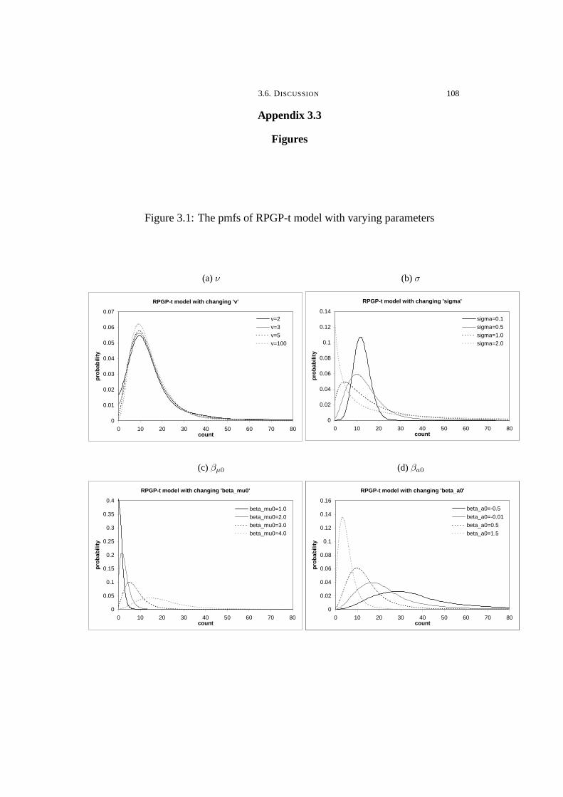
3.6. DISCUSSION 108
Appendix 3.3
Figures
Figure 3.1: The pmfs of RPGP-t model with varying parameters
(a) ν
RPGP-t model with changing 'v'
0
0.01
0.02
0.03
0.04
0.05
0.06
0.07
0 10 20 30 40 50 60 70 80count
pro
bab
ility
v=2v=3v=5v=100
(b) σ
RPGP-t model with changing 'v'
0
0.01
0.02
0.03
0.04
0.05
0.06
0.07
0 10 20 30 40 50 60 70 80count
pro
bab
ility
v=2v=3v=5v=100
RPGP-t model with changing 'sigma'
0
0.02
0.04
0.06
0.08
0.1
0.12
0.14
0 10 20 30 40 50 60 70 80count
pro
bab
ility
sigma=0.1sigma=0.5sigma=1.0sigma=2.0
(c) βµ0
RPGP-t model with changing 'beta_mu0'
0
0.05
0.1
0.15
0.2
0.25
0.3
0.35
0.4
0 10 20 30 40 50 60 70 80count
pro
bab
ility
beta_mu0=1.0beta_mu0=2.0beta_mu0=3.0beta_mu0=4.0
(d) βa0
RPGP-t model with changing 'v'
0
0.01
0.02
0.03
0.04
0.05
0.06
0.07
0 10 20 30 40 50 60 70 80count
pro
bab
ility
v=2v=3v=5v=100
RPGP-t model with changing 'beta_mu0'
0
0.05
0.1
0.15
0.2
0 10 20 30 40 50 60 70 80count
pro
bab
ility
beta_mu0=1.5beta_mu0=2.5beta_mu0=3.0beta_mu0=4.0
RPGP-t model with changing 'beta_a0'
0
0.02
0.04
0.06
0.08
0.1
0.12
0.14
0.16
0 10 20 30 40 50 60 70 80count
pro
bab
ility
beta_a0=-0.5
beta_a0=-0.01
beta_a0=0.5
beta_a0=1.5

3.6. DISCUSSION 109
Figure 3.2: The pmfs of RPGP-EP model with varying parameters
(a) ν
RPGP-EP model with changing 'v'
0
0.02
0.04
0.06
0.08
0.1
0 10 20 30 40 50 60 70 80count
pro
bab
ility
v=0.1v=0.5v=1.0v=2.0
(b) σ
RPGP-EP model with changing 'v'
0
0.02
0.04
0.06
0.08
0.1
0 10 20 30 40 50 60 70 80count
pro
bab
ility
v=0.1v=0.5v=1.0v=2.0
RPGP-EP model with changing 'sigma'
0
0.02
0.04
0.06
0.08
0.1
0.12
0.14
0 10 20 30 40 50 60 70 80count
pro
bab
ility
sigma=0.1sigma=0.5sigma=1.0sigma=2.0
(c) βµ0
RPGP-EP model with changing 'v'
0
0.02
0.04
0.06
0.08
0.1
0 10 20 30 40 50 60 70 80count
pro
bab
ility
v=0.1v=0.5v=1.0v=2.0
RPGP-EP model with changing 'sigma'
0
0.02
0.04
0.06
0.08
0.1
0.12
0.14
0 10 20 30 40 50 60 70 80count
pro
bab
ility
sigma=0.1sigma=0.5sigma=1.0sigma=2.0
RPGP-EP model with changing 'beta_mu0'
0
0.05
0.1
0.15
0.2
0.25
0.3
0.35
0 10 20 30 40 50 60 70 80count
pro
bab
ility
beta_mu0=1.0
beta_mu0=2.0
beta_mu0=3.0
beta_mu0=4.0
(d) βa0
RPGP-EP model with changing 'beta_a0'
0
0.02
0.04
0.06
0.08
0.1
0.12
0.14
0.16
0.18
0 10 20 30 40 50 60 70 80count
pro
bab
ility
beta_a0=-0.5
beta_a0=-0.01
beta_a0=0.5
beta_a0=1.5

3.6. DISCUSSION 110
Figure 3.3: pmf of 2-group RMPGP-EP model at t = 1
GPGP model with changing 'lambda2'
0
0.02
0.04
0.06
0.08
0.1
0.12
0 10 20 30 40 50count
pro
bab
ility
lambda2=-0.5lambda2=-0.2lambda2=0.2lambda2=0.5
GPGP model with changing 'r'
0
0.02
0.04
0.06
0.08
0 10 20 30 40 50 60count
pro
bab
ility
r=1.2
r=2
r=8
r=40
pmf of 2-group RMPGP-EP model at t=1
0
0.01
0.02
0.03
0.04
0.05
0.06
0.07
0.08
0 20 40 60 80 100 120count
pro
bab
ility
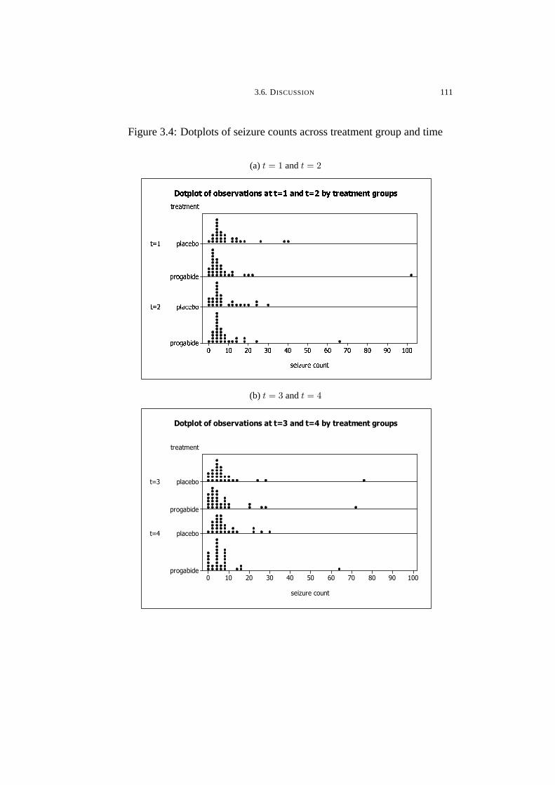
3.6. DISCUSSION 111
Figure 3.4: Dotplots of seizure counts across treatment group and time
(a) t = 1 and t = 2
������ �� ����� ������ �� �� ��
� ������� �������
��� �
��� �
��� ���������
� ����������� ���
��� ���������
� ����������� ���
��� !#"��$���#��"����
%'&)(�*)+�&,(-&).-&,/,021)3�4,5)(�6$&,7,085,(-(:98;<5)7,=>(?9A@B/)CD(#3�1)5)(�ED1)7)(GF)3�&)H,*)0
(b) t = 3 and t = 4
�� �� �� �� �� �� �� � � ����
� � � � � � �
� �
� � �
� � � � � �
� � � � � � � �
� � � � � �
� � � � � � � �
� � � � � � � � � � �
�� � � � � � � � � � � � � � � � � � � � � � � � � � � � � � � � � � � � � � � � � � � � � � �

3.6. DISCUSSION 112
Figure 3.5: The pmfs of low-level group for RMPGP models at different
times
(a) t = 1
Observed and fitted pmfs of low-level group at t=1
0
0.05
0.1
0.15
0.2
0.25
0 1 2 3 4 5 6 7 8 9 10 11 12 13 14
seizure count
pro
bab
ility
t-observed EP-observed t-fitted EP-fitted
(b) t = 2
Observed and fitted pmfs of low-level group at t=1
0
0.05
0.1
0.15
0.2
0.25
0 1 2 3 4 5 6 7 8 9 10 11 12 13 14
seizure count
pro
bab
ility
t-observed EP-observed t-fitted EP-fitted
Observed and fitted pmfs of low-level group at t=2
0
0.05
0.1
0.15
0.2
0.25
0.3
0 1 2 3 4 5 6 7 8 9 10 11 12 13 14
seizure count
pro
bab
ility
t-observed EP-observed t-fitted EP-fitted
(c) t = 3
Observed and fitted pmfs of low-level group at t=1
0
0.05
0.1
0.15
0.2
0.25
0 1 2 3 4 5 6 7 8 9 10 11 12 13 14
seizure count
pro
bab
ility
t-observed EP-observed t-fitted EP-fitted
Observed and fitted pmfs of low-level group at t=2
0
0.05
0.1
0.15
0.2
0.25
0.3
0 1 2 3 4 5 6 7 8 9 10 11 12 13 14
seizure count
pro
bab
ility
t-observed EP-observed t-fitted EP-fitted
Observed and fitted pmfs of low-level group at t=3
0
0.05
0.1
0.15
0.2
0.25
0 1 2 3 4 5 6 7 8 9 10 11 12 13 14
seizure count
pro
bab
ility
t-observed EP-observed t-fitted EP-fitted
(d) t = 4
Observed and fitted pmfs of low-level group at t=4
0
0.05
0.1
0.15
0.2
0.25
0 1 2 3 4 5 6 7 8 9 10 11 12 13 14
seizure count
pro
bab
ility
t-observed EP-observed t-fitted EP-fitted
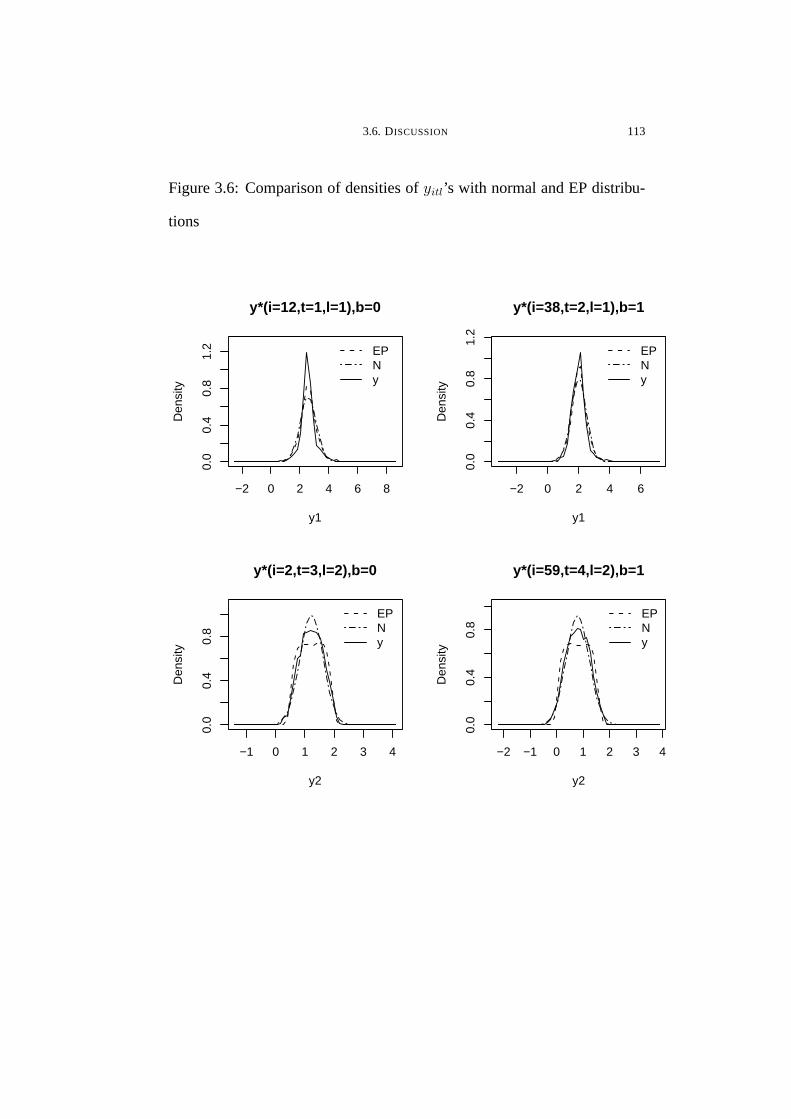
3.6. DISCUSSION 113
Figure 3.6: Comparison of densities of yitl’s with normal and EP distribu-
tions
−2 0 2 4 6 8
0.0
0.4
0.8
1.2
y1
Den
sity
y*(i=12,t=1,l=1),b=0
EPNy
−2 0 2 4 6
0.0
0.4
0.8
1.2
y1
Den
sity
y*(i=38,t=2,l=1),b=1
EPNy
−1 0 1 2 3 4
0.0
0.4
0.8
y2
Den
sity
y*(i=2,t=3,l=2),b=0
EPNy
−2 −1 0 1 2 3 4
0.0
0.4
0.8
y2
Den
sity
y*(i=59,t=4,l=2),b=1
EPNy

3.6. DISCUSSION 114
Figure 3.7: Outlier diagnosis using uitl in the RMPGP-EP model
Outlier detection for RMPGP-EP model
0
2
4
6
8
10
0 40 80 120 160 200 240
observation
w'_
itl a
nd
u_i
tl
w (high-level)w (low-level)top 10 u (w)u (high-level)u (low-level)
1 (102)
3 (72)2 (63)
4 (65)
5 (0) 7 (1)8 (2)
6 (76)
10 (40) 9 (2)
CHAPTER 4
Generalized Poisson geometric process model
PGP model has been extended to allow for overdispersion that is caused,
in particular, by zero-inflation in Chapter 2 and extreme observations in
Chapter 3. This Chapter extends the PGP model in (1.4) to fit longitudinal
count data with more flexible degrees of dispersion ranging from underdis-
persion to overdispersion.
4.1. Background
Owing to the deficiency of the Poisson distribution that it can only han-
dle equidispersed count data, our primary objective is to develop a unified
model that can accommodate both overdispersion and underdispersion in
longitudinal and panel count data. Besides considering the degree of dis-
persion, our proposed model should also take into account the trend move-
ments, serial correlation between successive observations which is promi-
nent in time series of counts and cluster effects which are often detected
in repeated measures design. Throughout the history of count data mod-
elling, since most count data exhibits overdispersion due to outliers, excess
zero observations and population heterogeneity, enormous literature can be
found to deal with overdispersion by using different methods to introduce
extra-variation to the Poisson distribution.
115

4.1. BACKGROUND 116
One historic approach is to use the Poisson mixed distribution which
assumes that the mean of the Poisson distribution follows a suitable mixing
distribution. This mixed model approach was first considered by Green-
wood & Yule (1920) which adopted a gamma distribution as the mixing
distribution and resulted in the well-known negative binomial distribution.
Since then, a large number of mixing distributions are considered and some
benchmarking models include the Poisson-inverse Gaussian mixed model
(Holla, 1966), Poisson-lognormal mixed model (Blumer, 1974) and Poisson-
generalized gamma mixed model (Albrecht, 1984). See Karlis & Meligkot-
sidou (2005) for a detailed review.
Concerning overdispersion particularly due to zero-inflation, two strands
of models, namely the hurdle model and the zero-inflated model prevail in
the literature. The former class proposed by Mullahy (1986) first deter-
mines whether the outcome is zero or positive by a logistic model and then
conditional on positive outcome, models the positive counts by a truncated
discrete distribution, such as truncated Poisson or truncated negative bino-
mial distribution. On the contrary, the latter class introduced by Lambert
(1992) is regarded as a mixture of zero-truncated Poisson distribution and a
component that degenerates at zero. These models, which are designed for
cross-sectional count data, were later extended to fit longitudinal count data.
Adopting the hurdle model, Dobbie & Welsh (2001) incorporated a serial
dependence structure via a generalized estimating approach so that the mar-
ginal model structure can be preserved. On the other hand, Yau et al. (2003)

4.1. BACKGROUND 117
extended the zero-inflated Poisson model to zero-inflated negative binomial
mixed regression model by introducing random effects to account for serial
dependence between successive observations. Nevertheless, all these mod-
els have a component that adds extra variation to the Poisson distribution
and therefore fail to deal with underdispersion.
Compared to overdispersion, the analogous problem of underdispersion
relative to Poisson distribution has not received too much attention as it is
less frequently observed in longitudinal and panel count data. But ignoring
this problem will result in an overestimated variance and a misleading inter-
pretation on the volatility of the data. Amongst the limited literature, Faddy
(1997) proposed the birth process model based on a generalization of the
Poisson process and stated that the rate of process (birth rate) at any time
point is a function of time and depends on the current number of events.
In the birth process model, overdispersion/underdispersion is attained when
the rate of process is monotone increasing/decreasing with time. Besides
the birth process model, other alternative distributions that can allow un-
derdispersion include the Conway-Maxwell-Poisson distribution (Conway
& Maxwell, 1962), generalized Poisson distribution Consul & Jain (1973),
double Poisson distribution (Efron, 1986) and weighted Poisson distribution
Ridout & Besbeas (2004).
Amongst all the aforementioned distributions for underdispersion, the
generalized Poisson distribution (GPD) pioneered by Consul & Jain (1973)
received considerably more attention. Relative to Poisson distribution, the

4.1. BACKGROUND 118
two-parameter GPD contains an additional parameter to control the shape
of the distribution. The variance can be greater than, equal to or smaller
than the mean when the parameter is positive, zero or negative respectively.
Some extensions of the GPD distribution on cross-sectional count data in-
clude the generalized Poisson regression model (Consul & Famoye, 1992)
to incorporate covariate effect, the zero-inflated generalized Poisson regres-
sion model (Angers & Biswas, 2003) to deal with excess zeros and the
k-inflated generalized Poisson regression model (Bae et al., 2005) to han-
dle excessive k-valued observations. Until very recently, Xie et al. (2009)
extended the zero-inflated generalized Poisson regression model to analyze
correlated panel count data by incorporating a latent random effect to ac-
count for the serial dependence.
So far, the extension of the PGP models in the previous Chapters fo-
cuses only on overdispersion due to excess zeros in Chapter 2 and extreme
observations in Chapter 3. To relax such restriction, we extend in this Chap-
ter the PGP model to a more comprehensive model to handle longitudinal
and panel count data with different degrees of dispersion by replacing the
Poisson data distribution with GPD. The resultant model is named as the
generalized Poisson geometric process (GPGP) model. Moreover, regard-
ing our secondary objective, the GPGP model is further extended to the
mixture generalized Poisson geometric process (GMPGP) model to incor-
porate cluster effects and serial dependence.

4.2. MODEL SPECIFICATION 119
To demonstrate the model properties and applicability, the remainder of
this Chapter is presented as follows. First, the GPGP and GMPGP models
will be specified in Section 4.2 with a study of the model distribution. Next,
Section 4.3 will discuss the implementation of the GMPGP model using
MCMC algorithms followed by the introduction of the model assessment
criterion. After that, the properties and practicability of the GMPGP model
will be demonstrated through some simulation studies and real data analysis
in Sections 4.4 and 4.5 respectively with comparison to the RMPGP-EP
model (best model in Chapter 3). Lastly, Section 4.6 will give a summary
of all the important findings.
4.2. Model specification
This Section first presents the GPD. Then, the GPGP model is intro-
duced with a detailed examination of the model distribution.
4.2.1. Generalized Poisson distribution. The generalized Poisson dis-
tribution (GPD) was introduced by Consul & Jain (1973) and was investi-
gated in detail by Consul (1989). If a random variable W has a GPD, then
its probability mass function (pmf) denoted by fGPD(w|λ1, λ2) is given by:
fGPD(w|λ1, λ2) =
λ1(λ1 + λ2w)w−1 exp[−(λ1 + λ2w)]
w!, w = 0, 1, . . . ;
0, w > s when λ2 < 0(4.1)
where λ1, |λ2| < 1 and s ≥ 4 is the largest natural number such that λ1 +
λ2s > 0 when λ2 < 0. The two parameters λ1 and λ2 are subject to the
following constraints:

4.2. MODEL SPECIFICATION 120
1. λ1 ≥ 0
2. max{−1,−λ1
s} < λ2 < 1.
For the GPD, the mean and variance are given by:
E(W ) =λ1
1 − λ2
and V ar(W ) =λ1
(1 − λ2)3=
E(W )
(1 − λ2)2.
Obviously, the shape of the GPD is controlled by the parameter λ2. A nega-
tive λ2 indicates underdispersion, the mean is less than the variance, whilst
a positive λ2 indicates overdispersion. The GPD reduces to the equidis-
persed Poisson distribution when λ2 = 0. Moreover, the variance increases
or decreases at a faster rate than the mean when λ2 varies. Relative to the
Poisson distribution, this two-parameter GPD demonstrates a wider range
of shapes and thus can fit data with different degrees of dispersion.
4.2.2. Generalized Poisson geometric process model. Let Wit de-
notes the count for subject i at time t, i = 1, . . . ,m, t = 1, . . . , ni and
n =m∑
i=1
ni. Under the PGP framework, instead of using the Poisson distri-
bution, we assume that the count Wit follows GPD with mean E(Wit) =
Xit =λ1it
(1 − λ2). Without loss of generality, {Xit =
Yit
at−1, t = 1, . . . , ni}
forms a latent GP and Yit follows gamma distribution fG(yit| r, rµi
) with
mean µi and varianceµ2
i
r. So, conditional on λ2 > 0, the marginal pmf for
Wit becomes
f(wit) =
∫ ∞
0
fGPD(wit|λ1it, λ2)fG
(yit
∣∣∣∣ r,r
µi
)dyit
=
∫ ∞
0
(1 − λ2)rryr
it
[(1−λ2)yit
at−1 + λ2wit
]wit−1
exp{−[
(1−λ2)yit
at−1 + λ2wit + ryit
µi
]}
at−1µri Γ(r)wit!
dyit (4.2)
4.2. MODEL SPECIFICATION 121
where λ1it =(1 − λ2)yit
at−1. When λ2 < 0, the marginal pmf for Wit is
given by (4.2) when wit = 0, 1, . . . , sit and 0 when wit > sit. The resultant
model is named as generalized Poisson geometric process (GPGP) model.
Although there is no apparent simplification of the integral, its moment can
be easily derived through conditional expectation and the law of total vari-
ance. In particular, the unconditional mean E(Wit) and variance V ar(Wit)
of the GPGP model are given by:
E(Wit) = Ex[Ew(Wit|Xit)] = Ex(Xit) = Ey
(Yit
at−1
)=
µi
at−1(4.3)
V ar(Wit) = Ex[V arw(Wit|Xit)] + V arx[Ew(Wit|Xit)]
= Ex
[Xit
(1 − λ2)2
]+ V arx(Xit)
=µi
at−1(1 − λ2)2+
µ2i
a2(t−1)r=
µi
at−1
[1
(1 − λ2)2+
µi
at−1r
](4.4)
Clearly, µi and a control both the mean and variance while r and λ2 act as
the dispersion parameters as they only control the variance. Based on (4.4),
the larger the r and the more negative the λ2, the more underdispersed is the
distribution of the GPGP model. Hence, by varying the model parameters,
the GPGP model can be fitted to both overdispersed and underdispersed
data.
4.2.3. Incorporation of mixture effects. Despite different degrees of
dispersion, an adequate model for panel count data should account for pop-
ulation heterogeneity which often arises in repeated measures design, ac-
commodate time-evolving covariate effects and address trend movements

4.2. MODEL SPECIFICATION 122
which are usually detected in time series of counts. In light of these, we
first extend the GPGP model to the mixture GPGP (GMPGP) model as fol-
lows.
To account for population heterogeneity, we postulate that there are G
groups of subjects which have distinct trend patterns and each subject has a
probability πl of coming from group l, l = 1, . . . , G. The resultant GMPGP
model is essentially a mixture of G GPGP models in which each model is
associated with a probability πl. Secondly, concerning the covariate effects
and trend movements, let βjl = (βj0l, βj1l, . . . , βjqj l)T to be a vector of
regression parameters βjkl, j = µ, a; k = 0, . . . , qj; l = 1, . . . , G. The
mean µi and constant ratio a are extended to the mean function µitl and
ratio function aitl function respectively which can be log-linked to some
time-evolving covariates zjkit, i = 1, . . . ,m; t = 1, . . . , ni and they are
given by:
µitl = exp(βµ0l + βµ1lzµ1it + · · · + βµqµlzµqµit) (4.5)
aitl = exp(βa0l + βa1lza1it + · · · + βaqalzaqait). (4.6)
Then conditional on group l, the marginal pmf of the GMPGP model can
be extended from (4.2) when λ2l > 0 and becomes:
fl(wit) =
∫ ∞
0
(1 − λ2l)rrl
l yrl
itl
[(1−λ2l)yitl
at−1itl
+ λ2lwit
]wit−1
exp{−[
(1−λ2l)yitl
at−1itl
+ λ2lwit + rlyitl
µitl
]}
at−1itl µ
rl
itl Γ(rl)wit!dyitl. (4.7)

4.2. MODEL SPECIFICATION 123
When λ2l < 0, the marginal pmf for Wit is given by (4.7) for wit =
0, 1, . . . , sit and 0 for wit > sit. Based on (4.3) and (4.4), the mean El(Wit)
and variance V arl(Wit) conditional on group l become
El(Wit) =µitl
at−1itl
and V arl(Wit) =µitl
at−1itl (1 − λ2l)2
+µ2
itl
a2(t−1)itl rl
. (4.8)
4.2.4. Incorporation of serial correlation. As the outcomeWit in lon-
gitudinal and panel data is often serially correlated, an adequate count model
should be able to incorporate a flexible serial dependence structure. To
identify an appropriate serial dependence structure, we first fit a prelimi-
nary model and obtain the predicted value based on (4.8). Then the Pearson
residuals and test statistic are derived in a similar way to the RMPGP mod-
els mentioned in Section 3.3.4 by using El(Wit) and V arl(Wit) in (4.8).
If the residuals are serially correlated up to lag L, Dobbie & Welsh
(2001) and Yau et al. (2003) adopted the PD approach, which is known as
marginal model approach in Zeger et al. (1988), to incorporate serial de-
pendence by adding random effects into the model. However we adopt the
OD approach described in Section 1.2.1 by adding L lagged observations
as autoregressive (AR) terms in the mean function µitl in (4.5). The model
parameters will be re-estimated and the appropriateness of the assumed AR
structure is evaluated through the significance of the parameters for the AR
terms and the model selection criterion discussed in Section 4.3.2.
4.2.5. Approximation of distribution. Since the pmf in (4.7) does not
have a closed-form, we approximate it using Monte Carlo (MC) integration

4.2. MODEL SPECIFICATION 124
as described below. We hereafter drop the subscript i in the mean function
µitl since only treatment-specific covariates are considered in the forthcom-
ing simulation experiments and real data analysis. Conditional on covari-
ates zjkt = zjkit and time t, the pmf estimator ftl(w) with mean function µtl
and ratio function atl can be obtained by:
ftl(w) =Ms∑
j=1
fGPD
(w
∣∣∣∣∣y
(j)tl
at−1tl
, λ2l
)
=Ms∑
j=1
(1 − λ2l)y(j)tl
[(1−λ2l)y
(j)tl
at−1tl
+ λ2lw
]w−1
exp
{−[
(1−λ2l)y(j)tl
at−1tl
+ λ2lw
]}
at−1tl w!
, w = 0, 1, ...,∞;
y(j)tl ∼ fG
(y
(j)tl
∣∣∣∣µtl,rl
µtl
), j = 1, . . . ,Ms (4.9)
where Ms is the number of simulations and the latent y(j)tl are simulated
from gamma distribution given the shape parameter rl. The mean El(Wt)
and variance V arl(Wt) of the approximated pmf ftl(w) for group l and time
t are calculated by:
El(Wt) =∞∑
w=0
wftl(w) and V arl(Wt) =
[∞∑
w=0
w2ftl(w)
]− [El(Wt)]
2 (4.10)
and are compared with the values obtained in (4.8) to assess the perfor-
mance of the MC integration.
To study the pmfs of the proposed GPGP model, we assume G = 1,
m = 1, qµ = qa = 1, zµ1t = b = 0, 1 as the covariate effect in (4.5) and
za1t = t as the time-evolving covariate effect in (4.6). Hence dropping the
subscript l in (4.9) since G = 1, the mean function is µt = exp(βµ0 + βµ1b)
and the ratio function is at = exp(βa0 + βa1t). Fixing b = 1 and t = 2,
4.2. MODEL SPECIFICATION 125
we change the values of one of the model parameters at one time while
keeping the other parameters constant and approximate the pmf in (4.2)
using MC integration described in (4.9) with Ms = 10000. The marginal
pmfs are displayed in Figures 4.1(a) to 4.1(d) in Appendix 4.3 with their
means and variances summarized in Table 4.1 in Appendix 4.2. The mean
and variance of the approximated pmf ft(w) are calculated using (4.10)
(dropping the subscript l) and are compared to the true values obtained from
(4.3)-(4.4). Note that since different pmfs are drawn on the same graph for
comparison, we use curves instead of bars to represent the marginal pmfs
for better visualization.
====================================
Figures 4.1(a) to 4.1(d) and Table 4.1 about here
====================================
The close affinity between E(Wt) & E(Wt) and V ar(Wt) & V ar(Wt)
in Table 4.1 confirms that the MC integration gives a satisfactory approxi-
mation of the pmfs for the GPGP model in (4.2). Based on the Figures and
results in Table 4.1, the parameters βµ0 and βa0 control both the location and
degree of dispersion of the distribution. A larger βµ0 and a smaller βa0 lead
to larger mean and variance of the resultant distribution. On the other hand,
r serves as a dispersion parameter. Without altering the mean, a smaller
r contributes to a larger variance for the distribution. Moreover, λ2 is an-
other important dispersion parameter which determines whether the distri-
bution shows an underdispersion, equidispersion or overdispersion. Note
4.3. BAYESIAN INFERENCE 126
that since the gamma distribution of the underlying stochastic process {Yt}
introduces extra variation to the GPD, a negative λ2 does not necessarily
reveal an underdispersion as shown in Table 4.1. For example, overdisper-
sion (E(Wt) < V ar(Wt)) is retained even when λ2 = −0.2. But in fact,
the variance is controlled by the factor1
(1 − λ2)2+
µt
at−1t r
based on (4.4).
In general, the more negative the λ2, the more underdispersed is the dis-
tribution. In summary, by varying the model parameters, the GPGP model
can fit count data with different degrees of dispersion, ranging from under-
dispersion due to the concentration of observations over a small range of
values to overdispersion due to some outlying observations.
4.3. Bayesian inference
For the statistical inference of generalized Poisson regression model,
maximum likelihood (ML) method (Bae et al., 2005) or moment method
(Consul & Jain, 1973) are used since the model has tractable likelihood
function. In the case when latent random effects are incorporated in the
model, Yau et al. (2003) adopted the expectation-maximization (EM) method.
However, since the likelihood function of the GMPGP model involves high-
dimensional integration, we avoid the numerical difficulties in maximiz-
ing the intractable likelihood function by using the Bayesian approach via
Markov chain Monte Carlo (MCMC) algorithms. Again, the MCMC al-
gorithms are implemented using WinBUGS. The next Section derives the
posterior distribution and univariate full conditional distributions followed
by a description of the model selection criterion.

4.3. BAYESIAN INFERENCE 127
4.3.1. MCMC algorithms. Before implementing the MCMC algorithms,
we outline the hierarchical structure of the GMPGP model under the Bayesian
framework as follows:
wit ∼ Ii1fGPD
(yit1
at−1it1
, λ21
)+ · · · + IiGfGPD
(yitG
at−1itG
, λ2G
)
yitl ∼ fG
(rl,
rl
µitl
)
where µitl and aitl are given by (4.5) and (4.6) and Iil is the group member-
ship indicator for subject i such that Iil = 1 if he/she comes from group l
and zero otherwise. In order to construct the posterior density, some non-
informative prior distributions are assigned to the model parameters as fol-
lows:
βjkl ∼ N(0, τ 2jkl), (4.11)
j = µ, a; k = 0, 1, . . . , qj; l = 1, . . . , G
rl ∼ Gamma(cl, dl) (4.12)
λ2l ∼ Uniform(−1, 1) (4.13)
(Ii1, . . . , IiG)T ∼ Multinomial(1, π1, . . . , πG) (4.14)
(π1, . . . , πG)T ∼ Dir(α1, . . . , αG) (4.15)
where cl, dl are some positive constants and Dir(α) represents a Dirich-
let distribution, a conjugate to multinomial distribution, with parameters
α = (α1, . . . , αG). Without prior information, we assign τ 2jkl = 1000 in
(4.11), cl = dl = 0.01 in (4.12) and αl = 1/G in (4.15) for a G-group

4.3. BAYESIAN INFERENCE 128
(G ≥ 2) model unless otherwise specified. In particular, for a 2-group
(G = 2) GMPGP model, (4.14) is simplified to Ii1 ∼ Bernoulli(π1) with
Ii2 = 1 − Ii1 and (4.15) becomes π1 ∼ Uniform(0, 1) with π2 = 1 − π1.
With the posterior means Iil of the group membership indicators Iil, patient
i is classified to group l′ if Iil′ = maxlIil.
According to Bayes’ theorem, the posterior density is proportional to
the joint densities of complete data likelihood and prior probability distri-
butions. For the GMPGP model, the complete data likelihood functionL(θ)
for the observed data wit and missing data {yitl, Iil} is derived as:
L(θ) =m∏
i=1
G∏
l=1
{πl
ni∏
t=1
fGPD(wit|βal, λ2l, yitl)fG(yitl|βµl, rl)
}Iil
.(4.16)
The vector of model parameters θ = (βT ,λT2 , r
T ,πT )T where β = (βTµ1, ...,
βTµG,β
Ta1, ...,β
TaG)T = (βµ01, ..., βµqµG, βa01, ..., βaqaG)T , λ2 = (λ21, ..., λ2G)T ,
r = (r1, ..., rG)T and π = (π1, ..., πG)T .
Treating {yitl, Iil} as missing observations, the joint posterior density of
the GMPGP model is expressed as follows:
f(β,λ2, r,π|w, I,y) ∝ L(θ)
(∏
j=µ,a
qj∏
k=0
G∏
l=1
fN(βjkl| 0, τ 2jkl)
)(G∏
l=1
fG(rl| cl, dl)
)
(G∏
l=1
fU(λ2l| − 1, 1)
)fDir(π|α)
where w = (w11, w12, ..., wmnm)T , I = (I11, I12, ..., ImG)T and y = (y111, y121, ..., ymnmG)T .
The complete data likelihood L(θ) of the GMPGP model is given by (4.16)
and the priors are given by (4.11)-(4.15). In Gibbs sampling, the unknown

4.3. BAYESIAN INFERENCE 129
parameters are simulated iteratively from their univariate conditional pos-
terior distributions which are proportional to the joint posterior density of
complete data likelihood and prior densities.
The univariate full conditional posterior densities for each of the un-
known model parameters θ and missing observations y and I are given by:
f(βµkl|w, I,y,β−,λ2, r,π) ∝ exp
[−
m∑
i=1
Iil
ni∑
t=1
(rlβµklzµkit +
rlyitl
µitl
)−
β2µkl
2τ 2µkl
]
f(βakl|w, I,y,β−,λ2, r,π) ∝m∏
i=1
ni∏
t=1
{[yitl(1 − λ2l)
at−1itl
+ λ2lwit
]wit−1
exp
[−yitl(1 − λ2l)
at−1itl
− βaklzakit(t− 1)
]}Iil
exp
(− β2
akl
2τ 2akl
)
restricted to at−1itl < −yitl(1 − λ2l)
sitλ2l
if λ2l < 0
f(yitl|w, I,y−,β,λ2l, r,π) ∝{yrl
itl
[yitl(1 − λ2l)
at−1itl
+ λ2lwit
]wit−1
exp
[−yitl(1 − λ2l)
at−1itl
− rlyitl
µitl
]}Iil
restricted to yitl > −sitλ2lat−1itl
1 − λ2l
if λ2l < 0
f(λ2l|w, I,y,β,λ−2l, r,π) ∝
m∏
i=1
ni∏
t=1
{(1 − λ2l)
[yitl(1 − λ2l)
at−1itl
+ λ2lwit
]wit−1
exp
[−yitl(1 − λ2l)
at−1itl
− λ2lwit
]}Iil
restricted to
(1 − sita
t−1itl
yitl
)−1
< λ2l < 1
f(rl|w, I,y,β,λ2, r−,π) ∝
m∏
i=1
ni∏
t=1
[rrl
l yrl
itl
µrl
itlΓ(rl)exp
(−rlyitl
µitl
)]Iil
rcl−1l exp(−rl dl)
f(πl|w, I,y,β,λ2, r,π−) ∝ π
mPi=1
Iil+αl−1
l

4.3. BAYESIAN INFERENCE 130
f(I i|w, I−,y,β,λ2, r,π) ∝
G∏
l=1
πl
ni∏t=1
(rlyitl)rl (1−λ2l)
µrlitl
Γ(rl)at−1itl
[yitl(1−λ2l)
at−1itl
+ λ2lwit
]wit−1
e−
„yitl(1−λ2l)
at−1itl
+λ2lwit+rlyitlµitl
«
G∑l′=1
πl′
ni∏t=1
(rl′yitl′ )rl′ (1−λ2l′ )
µrl′
itl′Γ(rl′)a
t−1itl′
[yitl′ (1−λ2l′ )
at−1itl′
+ λ2l′wit
]wit−1
e−
yitl′
(1−λ2l′)
at−1itl′
+λ2l′wit+rl′
yitl′
µitl′
!
Iil
=G∏
i=1
π′ Iil
il = Multinomial(1, π′i1, . . . , π
′iG)
where β−,y−,λ−2 , r
−,π− and I− are vectors of β,y,λ2, r,π and I ex-
cluding βjkl, yitl, λ2l, rl, πl and I i = (Ii1, . . . , IiG)T respectively. Neverthe-
less, the MCMC algorithms are implemented using the user-friendly soft-
ware WinBUGSwhere the sampling scheme based on the conditional poste-
rior densities is outlined in this Section and the Gibbs sampling procedures
are described in Section 1.4.3 and the posterior sample medians are adopted
as parameter estimates.
4.3.2. Model selection criterion. In this analysis, we adopt the de-
viance information criterion (DIC), originated by Spiegelhalter et al. (2002),
as the model selection criterion. For the GPGP model, the DIC is defined
as
DIC = D(θ) + pD
= − 4
M
M∑
j=1
m∑
i=1
G∑
l=1
I′(j)il
{lnπ
(j)l +
ni∑
t=1
ln[fGPD(wit| y(j)
itl ,β(j)al , λ
(j)2l )fG(y
(j)itl |β
(j)µl , r
(j)l )]}
+2m∑
i=1
G∑
l=1
I ′il
{ln πl +
ni∑
t=1
ln[fGPD(wit| yitl, βal, λ2l)fG(yitl| βµl, rl)
]}
(4.17)

4.4. SIMULATION STUDIES 131
where θ(j) and θ represent the jth posterior sample and posterior mean of
parameter θ respectively,
I′(j)il =
π(j)l
ni∏t=1
{fGPD(wit| y(j)
itl ,β(j)al , λ
(j)2l )fG(y
(j)itl |β
(j)µl , r
(j)l )}
G∑l′=1
π(j)l′
ni∏t=1
[fGPD(wit| y(j)
itl′ ,β(j)al′ , λ
(j)2l′ , )fG(y
(j)itl′ |β
(j)µl′ , r
(j)l′ )] ,
and I ′il is defined in a similar way by replacing y(j)itl and θ(j) with yitl and θ.
For model selection, the best model should give the smallest DIC indicat-
ing it has the best fit after accounting for the model complexity.
4.4. Simulation studies
The objectives of the simulation studies are twofold: (1) to compare
the similarities and differences in the properties of the GPGP model and
the RPGP-EP model introduced in Chapter 3 and (2) to assess the compe-
tence of the two models under different levels of dispersion. Regarding the
first objective, we performed a ‘cross’ simulation study. For the second ob-
jective, the two models were fitted to some data with different degrees of
dispersion. The procedures and results of these studies are discussed in the
next two Sections.
4.4.1. Comparisons between GPGP and RPGP models. We conducted
some cross simulations in which data simulated from one model is ‘cross’-
fitted by both models. By setting G = 1 and qµ = qa = 1, h = 100 data sets
are simulated from each of the GPGP model in (4.7) or RPGP-EP model in
(3.12) with the true parameters given in Table 4.2 in Appendix 4.2, and they
are fitted using both GPGP and RPGP-EP models. Each data set contains
4.4. SIMULATION STUDIES 132
m = 80 time series of length ni = 8 from m0 = 40 subjects in the control
group (b = 0) and another m1 = 40 subjects in the treatment group (b = 1).
In both GPGP and RPGP-EP models (dropping subscript l since G = 1),
the treatment effect zµ1it = b is adopted in the mean functions in (4.5) and
(3.2) and time (za1it = t) is incorporated as the time-evolving effect in and
the ratio functions in (4.6) and (3.3). In addition, different values are as-
signed to βµk and βak, k = 0, 1 to give different trend patterns and baseline
levels. Moreover, the dispersion parameter ν of the RPGP-EP model is set
to be 0.1 to attain overdispersion in data set 1 and λ2 of the GPGP model is
set to be -0.99 to acquire underdispersion in data set 2.
Implemented using WinBUGS and R2WinBUGS with non-informative
priors as described in Section 4.3.1 for the GPGP model and Section 3.4 for
the RPGP-EP model, the parameter estimate θ is calculated as the average of
h = 100 posterior medians θ(j) in the jth data set. To examine the precision
of the MCMC sampling algorithms, the standard deviation (SD) of θ(j) over
h = 100 simulated data sets for each parameter θ is evaluated. To assess
the accuracy of parameter estimates when the data set is simulated from and
fitted by the same model, we calculate the mean squared error (MSE) for
each parameter θ which is given by:
MSE =1
h
h∑
j=1
(θ(j) − θ)2.
For model assessment, the average DIC is used to measure the goodness-
of-fit of the model while taking into account the model complexity. For

4.4. SIMULATION STUDIES 133
the GPGP model, DIC is computed using (4.17) while that of the RPGP-
EP model is calculated by (3.19). Table 4.2 summarizes the results of this
cross simulation study including the true parameters under different models
and various model assessment criteria such as the SD, MSE and DIC.
The reasonably small SD and MSE for all the parameters reflect that the
MCMC algorithms give precise and unbiased estimates except for r which
has a larger MSE due to its relatively larger magnitude of the estimate.
To demonstrate the level of dispersion in each data set, we approximated
the pmfs ft(w) based on the sets of true parameters (true model) and fitted
parameters (GPGP and RPGP-EP models) using MC integration described
in (4.9) for the GPGP model and in (3.5) for the RPGP-EP model. Based
on ft(w), the mean and variance of the true models, GPGP and RPGP-EP
models are calculated and reported in Table 4.3 in Appendix 4.2. Note that
unlike the GPGP model, the unconditional mean and variance of the RPGP-
EP model cannot be expressed explicitly as in (4.3) and (4.4) because {Yit}
follows log-uniform distribution. For fair comparison we therefore evaluate
the mean E(Wt) and variance V ar(Wt) using (4.10) based on the approxi-
mated pmfs ft(w) in the MC integration for both models in the sequel.
As indicated in Table 4.3, for data set 1, the overall variance of the true
pmfs is 2.53 which is larger than the overall mean 2.05 showing overdis-
persion. Based on the estimates of βa and βµ, the true mean shows a
gradually increasing trend till t = 3 and a substantially decreasing trend
afterwards. This non-monotone trend is well captured by the GPGP and

4.4. SIMULATION STUDIES 134
RPGP-EP models. Besides, the two models give similar mean and variance
across time and are comparable to those of the true model. These results re-
veal that both models can cope with overdispersed count data and therefore
they have similar average DIC with the GPGP model slightly outperform-
ing the RPGP-EP model (1828.3 versus 1860.4) in Table 4.2.
==================================
Tables 4.2 and 4.3 about here
==================================
On the other hand, in data set 2, the overall variance (1.31) of the true
pmfs is less than the overall mean (3.5) showing underdispersion. This
time the trend is generally increasing but turns downwards after t = 5.
Although both models can describe the non-monotone trend pattern, the
RPGP-EP model which cannot accommodate underdispersed data shows
a poor model fit with a substantially larger average DIC than the GPGP
model (1756.6 versus 2178.7) in Table 4.2. In addition, the variance of the
RPGP-EP model is inevitably larger than that of the true model as the fur-
thest degree of dispersion this model can attain is only equidispersion. This
explains why the mean of the RPGP-EP model is underestimated across
time. On the contrary, the GPGP model shows an overwhelming advantage
over the RPGP-EP model in fitting underdispersed data as supported evi-
dently by the affinity in the variance between the GPGP and true models in
Table 4.3.

4.4. SIMULATION STUDIES 135
This simulation study highlights the fact that while the two models
are competitive in dealing with overdispersed data, only the GPGP model
which has a more flexible dispersion structure is suitable for analyzing un-
derdispersed data.
4.4.2. Assessment of level of dispersion. In the second part of the sim-
ulation studies, one data set was selected from the data set 2 which is sim-
ulated from the GPGP model in the cross simulation study as described in
the previous Section with true parameters given in Table 4.2. This data set
which exhibits an underdispersion across time as revealed by the mean and
variance in Table 4.4 in Appendix 4.2 was fitted to both GPGP and RPGP-
EP models. Results in Table 4.5 show that the GPGP model consistently
gives a better model fit since it can allow for underdispersion while the
RPGP-EP model fails to do so.
Two more data sets were then generated by adding some outliers in
order to make the data distribution become equidispersed and overdispered
(see Table 4.4). More specifically, we add a constant to all observations of
the last subject in both control group (i = 40) and treatment group (i =
80) to study the responses of model parameters to the presence of outlying
values. Without altering the overall trend and with a slight increase in the
overall mean across time, the data distribution becomes equidispersed by
adding a constant nine and overdispersed by adding a constant fifteen.

4.4. SIMULATION STUDIES 136
In the case of equidispersion, for the RPGP-EP model, the parameters
of the mean and ratio functions do not alter too much since the trend move-
ment remains unchanged and the level of time series only increases slightly.
As expected, the shape parameter ν for {Y ∗it = lnYit} has changed sharply
from 0.15 to 0.88 and the scale parameter σ has increased moderately.
These imply that the distribution of the underlying latent stochastic pro-
cess {Y ∗it} becomes more heavy-tailed and overdispersed to accommodate
the outlying observations. While for the GPGP model, again the parame-
ters in the mean and ratio functions remain nearly stagnant except for the
shape parameter r of {Yit} which drops abruptly to allow for the inflated
variance due to the enlarged observations. The dispersion parameter λ2 in
the GPGP model however does not increase but instead becomes slightly
more negative, due to the fact that the variance of the distribution is con-
trolled by the factor1
(1 − λ2)2+
µt
at−1t r
, which involves both λ2 and r as
shown in (4.4). This reveals that the shape parameter r of the gamma dis-
tribution for {Yit} has a stronger effect than the dispersion parameter λ2
in the GPD for the outcome {Wit} on the level of dispersion and the de-
crease in r ‘absorbs’ the outlying effect by increasing the tailedness of the
model distribution. On the contrary, the RPGP-EP model downweighs the
outlying effect by increasing the shape parameter ν of the EP distribution
for {Y ∗it}. Comparing the model fit with the first case of underdispersion,
the DIC shows a substantially larger percentage change for the RPGP-EP

4.4. SIMULATION STUDIES 137
model (2.6% versus 10.4%) indicating that the GPGP model still performs
better in the situation of equidispersion.
In the case of overdispersion, the parameters show similar movements
with a dramatic increase in ν in the RPGP-EP model (0.88 to 1.98) and a fur-
ther decrease in r in the GPGP model (6.11 to 4.09). However this time the
percentage increase in the DIC compared with the situation of equidisper-
sion for both models becomes closer because they both can handle overdis-
persed data by increasing the tailedness of the model distribution, in dif-
ferent ways. In the RPGP-EP model, the outlying effect is downweighed
by widening the interval of the uniform distribution of the underlying latent
stochastic process {Y ∗it} whereas in the GPGP model, it is accommodated
by magnifying the variance of {Yit}.
Lastly we also investigate the case of zero-inflation, a common source
of overdispersion. To compare the performance of the two models in mod-
elling zero-inflated data with a high proportion of zeros, we simulated a
data set with the same structure mentioned at the beginning of Section 4.4.1
from the zero-inflated GPGP model with the following pmf:
fz(wit) =
φ+ (1 − φ)f(wit), when wit = 0
(1 − φ)f(wit), when wit > 0
where f(wit) is given by (4.2), φ = 0.5, βµ0 = 2.0, βµ1 = −0.5, βa0 =
0.8, βa1 = −0.1, λ2 = 0.2 and r = 1.0. The data set simulated from
the zero-inflated GPGP model has a high percentage of zeros observations
(78%) which leads to overdispersion and a U-shaped trend pattern as shown

4.5. REAL DATA ANALYSIS 138
in Table 4.4. Not surprisingly, since both models can cope with overdis-
persed data, the model fits of the two models indicated in Table 4.5 are
close with the GPGP model marginally outperforms the RPGP-EP model.
The dispersion parameter λ2 = 0.39 in the GPGP model and the shape pa-
rameter ν = 1.95 in the RPGP-EP model also agree with each other and
confirm overdispersion.
==================================
Tables 4.4 and 4.5 about here
==================================
In sum, the two simulation studies manifest the pitfall of RPGP-EP
model in modelling underdispersed data. On the contrary, GPGP model
is more comprehensive as it can fit data with different degrees of disper-
sion by varying the two model parameters λ2 and r. As the two simulation
studies have revealed the satisfactory performance of the GPGP model, its
practicability will be demonstrated in the following real data analysis.
4.5. Real data analysis
In this Section, the applicability of the GMPGP model is illustrated via
a panel data analysis of the arrest for cannabis use in New South Wales
(NSW), Australia. The background and the properties of the data are first
described. Then the results of the analysis and model comparison are inter-
preted in detail.

4.5. REAL DATA ANALYSIS 139
4.5.1. Overview. Cannabis is a recreational drug with few toxic acute
effects compared to other illicit drugs. The prevalence of canabbis use
is high as it gives users a sense of mild euphoria and relaxation but also
has some short-term side effects such as drowsiness and loss of coordina-
tion. An overdose of cannabis will exert deleterious effect on motor skills
and reaction time causing road traumas (Jones et al., 2005). Besides, the
cannabis abusers and quitters will experience paranoia and other withdrawal
symptoms which make them feel irritated or make them become aggressive.
These may result in violent behaviours and assaults and consequently lead
to mounting crime rates.
Unfortunately, the arrest of cannabis use was not effective as recognized
by the NSW Drug Summit. To alleviate this problem, the NSW Police and
Drug and Alcohol Coordination initiated the Cannabis Cautioning Scheme
in April 2000 to assist offenders to consider the legal and health ramifica-
tions of their cannabis use and seek treatment and support (Baker & Goh,
2004). Under this scheme, first- and second-time offenders who are caught
using or possessing of not more than 15g of dried cannabis would receive a
formal police caution rather than facing criminal charges and court proceed-
ings. The caution includes information about the consequence of cannabis
use and access to treatment and support services. It was expected that the
scheme could reduce the number of cannabis users throughout the state but
this effect still remained skeptical (Baker & Goh, 2004).

4.5. REAL DATA ANALYSIS 140
The objective of this data analysis is to evaluate the effectiveness of
the policy through the study of trend movement of the number of arrests for
dealing and trafficking of cannabis in NSW during 2001 to 2008. The data is
available on the official website of the NSW Bureau of Crime Statistics and
Research (http://www.bocsar.nsw.gov.au/lawlink/bocsar/ll_bocsar.nsf/pages/
bocsar_onlinequeries) and is described as follows.
4.5.2. Data and model fitting. The data set contains 344 yearly num-
ber Wit of arrests for cannabis dealing and trafficking from 2001 to 2008
in 43 local government areas (LGAs) within Sydney, the metropolitan re-
gion of NSW with the highest prevalence of drug dealing and trafficking
amongst all NSW divisions. This results in m = 43 time series in which
each consists of eight yearly counts (ni = 8) as reported in Appendix 4.1.
Clearly, the data exhibits cluster effects and overdispersion due to the
fact that some LGAs like Sydney, Bankstown, Blacktown, Campbelltown,
have significantly higher number of arrests for cannabis dealing and traf-
ficking throughout the studying period. Therefore, we incorporate mixture
effects into the model as described in Section 4.2.3. We postulate that there
exists G groups of LGAs in which each of the groups has distinct level of
arrests and trend pattern. Without any prior information about the num-
ber of groups that can be classified from the data, we fit the model with
G = 1, 2, . . . ,m group(s) and determine the value of G by assessing the
DIC and the significance of the model parameters. Moreover, the time se-
ries generally shows a decreasing trend during 2001 to 2004, stabilizes in

4.5. REAL DATA ANALYSIS 141
2004-2005 followed by a further drop in 2005-2007 but rebounds slightly
in 2008. In view of these characteristics and the desire to examine the com-
petence of the GMPGP model in handling overdispersed data by comparing
with the RMPGP-EP model, we fitted both GMPGP and RMPGP-EP mod-
els to the data taken into account the non-monotone trend patterns, overdis-
persion and population heterogeneity.
Considering the non-monotone trends, we incorporate a time evolving
effect za1it = ln t in the ratio function aitl in (4.6). Since there is no measure
of covariate effect on the trend level in the data, we simply set the mean
function µitl = βµ0l. Regarding the cluster effects, as we have no prior
information about the number of groups in the panel data, we fitted the
GMPGP models with G = 1, 2, 3, . . . ,m group(s) respectively using the
MCMC algorithms described in Section 4.3.1. For the priors, we specify
cl = 0.1, d1 = 0.05 and d2 = 0.1 in (4.12) while other hyperparameters
are specified as described in Section 4.3.1. The results of the analysis are
elaborated in the following Section.
4.5.3. Results. The 1-group GMPGP model (G = 1) fails to explain
the population heterogeneity leaving a large deviation between the observed
and predicted counts for some LGAs with high occurrences of cannabis
dealing and trafficking. This poor fit is revealed from the larger DIC
(3788.36) of the 1-group GMPGP model when compared to that of the 2-
group GMPGP model (DIC = 3751.78). However, a 3-group GMPGP
model (G = 3) overfits the data with one cluster actually degenerating.

4.5. REAL DATA ANALYSIS 142
Therefore we stop the model fitting process at G = 3 and confirm that
the 2-group GMPGP model (G = 2) is the most appropriate one to fit the
data and further fit a 2-group RMPGP-EP model for model comparison. In
addition, we find that the parameters βa1l, l = 1, 2 in the ratio functions
are insignificant (95% CI for βa1l contains zero) for both models indicating
that the trends are indeed monotone in both groups. Hence we drop the re-
dundant time-evolving covariate ln t in the ratio functions and they become
aitl = exp(βa0l). In Appendix 4.2, Table 4.6 summarizes the parameter
estimates, standard errors (SE) and model selection criterion DIC for the
GMPGP and RMPGP-EP models.
==================================
Table 4.6 about here
==================================
In the two fitted models, two distinct groups of LGAs are identified,
namely the high-level (l = 1) and low-level (l = 2) groups since the ini-
tial trend of the former group is higher across time (βµ01 > βµ02). For
the GMPGP model, the high-level group (l = 1) demonstrates a station-
ary trend since βa01 is not significantly different from zero (95% CI for
βa01:[−0.0062, 0.1033]) while the trend low-level group (l = 2) shows
a monotone declining trend (95% CI for βa02:[0.0326, 0.1493]). For the
RMPGP-EP model, both high-level and low-level groups exhibit a mono-
tone decreasing trend as the two parameters βa01 (95% CI:[0.0095, 0.1344])
and βa02 (95% CI:[0.0401, 0.1528]) are significantly greater than zero.

4.5. REAL DATA ANALYSIS 143
Concerning the classification, the LGA i is classified to group l, l =
1, 2 if the posterior mean Iil = maxl′
Iil′ . With respect to the GMPGP
model, 15 LGAs are categorized to the high-level group (l = 1) with
Ii1 = maxl′
Iil′ and as expected Sydney which is the central business district
with a high concentration of pubs and night clubs belongs to this group.
Most of the LGAs classified in this group, including Bankstown, Canter-
bury, Fairfield, Liverpool, Parramatta, Holroyd, Penrith and Blacktown, are
located in the central or outer west of Sydney. While a few of them like
Baulkham Hills, Gosford and Wyong are situated in northern Sydney, only
two LGAs, Hurstville and Sutherland Shire are located in the south and one
LGA, Campbelltown in the southwest. The categorization implies that the
arrests for cannabis dealing and trafficking are concentrated in the inner and
western part of Sydney. These results concur with the findings in Baker &
Goh (2004) that the number of charges laid for minor cannabis use in April
2001 to March 2003 were significantly higher in the inner metropolitan area
like Sydney and some western local area commands like Bankstown, Par-
ramatta, Holroyd, Penrith and Blacktown.
The classification of the LGAs in the RMPGP-EP model are nearly
identical except that 2 more LGAs, Marrickville in the inner Sydney area
and Waverley in the eastern Sydney area are categorized in the high-level
group. The affinity of the classification may possibly be due to the similar
way that the two models capture the population heterogeneity by incor-
porating mixture effects. Since the LGAs with outlying observations are

4.5. REAL DATA ANALYSIS 144
classified into the high-level group (l = 1), this group thus exhibits a higher
degree of overdispersion in contrast to the low-level group (l = 2) which
comprises of LGAs with low incidence counts. To verify this, we compare
the mean and variance over time of the two groups for both GMPGP and
RMPGP-EP models. To begin with, we evaluate the approximated pmfs
ftl(w) of the two groups using MC integration described in (4.9) for the
GMPGP model with atl = exp(βa0l) and µtl = exp(βµ0l). For the RMPGP-
EP model, ftl(w) is obtained by
ftl(w) =Ms∑
j=1
fP
(w
∣∣∣∣∣ey
∗(j)tl
at−1tl
)=
Ms∑
j=1
exp
(− e
y∗(j)tl
at−1tl
)(ey∗(j)tl
at−1tl
)w
w!, w = 0, 1, . . . ,∞; and
y∗(j)tl ∼ fEP (y
∗(j)tl |µ∗
tl, σl, νl), j = 1, . . . ,Ms
where fEP (·) is given by (3.6) and µ∗tl = βµ0l. Then we compute the ob-
served pmfs under the two models at different time t by:
ftl(w) =
m∑i=1
IilI(Wit = w)
∞∑w′=0
m∑i=1
IilIitl(Wit = w′), w = 0, 1, . . .
where I(Wit = w) = 1 if Wit = w and 0 otherwise and Iil is the posterior
mean of the membership indicator Iil for LGA i in group l. For both mod-
els, the predicted mean El(Wt) and variance V arl(Wt) are calculated using
(4.10). Similarly, the observed mean El(Wt) and variance V arl(Wt) are
computed by replacing ftl(w) with ftl(w). These means and variances are
reported in Table 4.7 in Appendix 4.2. Noticeably, the degree of overdis-
persion is substantially higher in the high-level group since some extreme

4.5. REAL DATA ANALYSIS 145
observations (w4,1 = 155, w4,2 = 114) in Sydney, one of the LGAs in this
group, inflate the variability of the counts dramatically. However, as both
GMPGP and RMPGP-EP models are robust to outliers and can downweigh
its influence in parameter estimation, the predicted variances of the high-
level group are underestimated in the first two years but are getting close to
the observed variances in the next six years for both models.
==================================
Table 4.7 about here
==================================
To investigate the trend movements, the distinct patterns for the two
groups are illustrated in Figure 4.2 in Appendix 4.3 by plotting the ob-
served mean El(Wt) and predicted mean El(Wt) under different models.
The Figure shows a declining trend in both high-level and low-level groups
with a relatively slower rate in the latter group. Moreover, the closeness
between the observed and predicted trends justify the adequacy of the mod-
els to fit the panel data. Overall, these results give statistical evidence that
the Cannabis Caution Scheme is associated with the drop in the number of
arrests for cannabis dealing and trafficking in NSW. In other words, our re-
sults imply that the Cannabis Caution Scheme is effective in reducing the
number of cannabis users within the Sydney metro area. This finding also
agrees with the 2007 National Drug Strategy Household Survey (Australian
Institute of Health and Welfare, 2008) that the proportion of the population
aged 14 years and over who had used cannabis in the last 12 months has

4.5. REAL DATA ANALYSIS 146
fallen from 15.8% in 2001 to 14.4% in 2004 and further reduced to 11.6%
in 2007.
====================================
Figure 4.2 about here
====================================
In the model comparison, after accounting for the model complexity, the
GMPGP model with a smaller DIC outperforms the RMPGP-EP model
and gives a better fit to the data. To explain this, we investigate the dif-
ference in model performance by comparing the observed pmf ftl(w) and
fitted pmf ftl(w) under the two models. Figures 4.3(a) and 4.3(b) in Ap-
pendix 4.3 display the observed and fitted pmfs of the high-level group in
both models at two chosen times t = 1 and t = 5. They clearly show that
the distribution of the GMPGP model has a heavier tail to accommodate
the outlying observations. The case is similar for the low-level group as
shown in Figures 4.4(a) and 4.4(b) in Appendix 4.3. Because of the heavier
tail, relative to the RMPGP-EP model, the GMPGP model generally gives
higher predicted counts and lower variances for both groups as revealed in
Table 4.7.
======================================
Figures 4.3(a), 4.3(b), 4.4(a) and 4.4(b) about here
======================================

4.5. REAL DATA ANALYSIS 147
Lastly, for the GMPGP model, the best model, according to the DIC,
we tested for the serial correlation using the procedures described in Sec-
tion 4.2.4. Starting from some lower lags, the p-values of the chi-square test
for autocorrelation up to lag 1,2 and 3 are 0.005, 0.015 and 0.124 respec-
tively. These results confirm the presence of serial correlation in the data
and therefore we refit the GMPGP model by including the AR(1) and AR(2)
terms into the mean function µitl. However, the AR(2) term in the high-level
group and all the AR terms in the low-level group are insignificant and thus
are discarded. The final model is the 2-group GMPGP model with an AR(1)
term incorporated into the mean function µit1 = exp(βµ01 + βµ11wi,t−1) for
the high-level group. The parameter estimates with SE for the final model
abbreviated as GMPGP-AR(1) model are reported in Table 4.7. Not sur-
prisingly, the parameter estimates are comparable to those of the GMPGP
model and the GMPGP-AR(1) model has a better DIC indicating that the
model fit has improved. Moreover, the significant positive βµ11 = 0.0198
implies that the current observation is positively correlated with the previ-
ous observation in the high-level group.
Last but not least, to illustrate their distinct trend movements and the
categorization of the LGAs in the GMPGP-AR(1) model, we plot the pre-
dicted individual and group trends for both high-level (l = 1) and low-level
(l = 2) groups in Figures 4.5(a) and 4.5(b) in Appendix 4.3. The predicted
number of arrest for cannabis dealing and trafficking for an individual LGA
i at time t is given by Wit = Ii1E1(Wit) + Ii2E2(Wit) where El(Wit) is

4.5. REAL DATA ANALYSIS 148
given by (4.8) and Iil is the posterior mean of the membership indicator
for group l, while that for the predicted group trend is simply given by a
weighted average of El(Wit) given by (4.10) with weight Iil for group l,
that is,
∑i IilEl(Wit)∑
i Iil. Note that for clearer visualization, Figure 4.5(b)
does not include the outlying predicted trend for the LGA, Sydney.
====================================
Figures 4.5(a) and 4.5(b) about here
====================================
Figure 4.5(a) vividly reveals that the LGA Sydney, though has a remark-
ably high number of arrests for cannabis dealing and trafficking, shows the
greatest drop throughout the entire studying period. While compared to
Sydney, other LGAs generally show a downward trend with a much slower
decreasing rate. Furthermore, Figure 4.5(b) shows the clear classification of
the LGAs by incorporating mixture effects into the model and the predicted
group trend in the high-level group demonstrates the ‘invulnerability’ of the
GMPGP-AR(1) model to extreme observations. In summary, the findings
with respect to the trend movements certainly provide useful information
for the allocation of police force to bring down the cannabis use especially
in those LGAs with higher number of arrests for cannabis dealing and traf-
ficking.
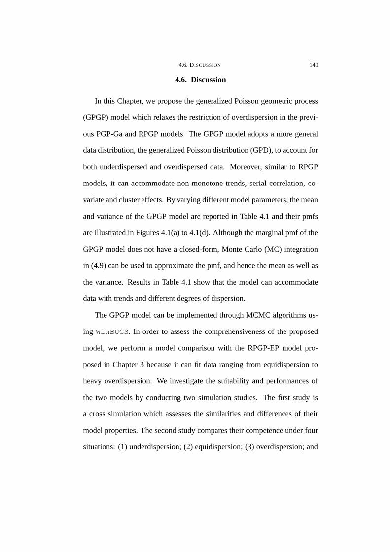
4.6. DISCUSSION 149
4.6. Discussion
In this Chapter, we propose the generalized Poisson geometric process
(GPGP) model which relaxes the restriction of overdispersion in the previ-
ous PGP-Ga and RPGP models. The GPGP model adopts a more general
data distribution, the generalized Poisson distribution (GPD), to account for
both underdispersed and overdispersed data. Moreover, similar to RPGP
models, it can accommodate non-monotone trends, serial correlation, co-
variate and cluster effects. By varying different model parameters, the mean
and variance of the GPGP model are reported in Table 4.1 and their pmfs
are illustrated in Figures 4.1(a) to 4.1(d). Although the marginal pmf of the
GPGP model does not have a closed-form, Monte Carlo (MC) integration
in (4.9) can be used to approximate the pmf, and hence the mean as well as
the variance. Results in Table 4.1 show that the model can accommodate
data with trends and different degrees of dispersion.
The GPGP model can be implemented through MCMC algorithms us-
ing WinBUGS. In order to assess the comprehensiveness of the proposed
model, we perform a model comparison with the RPGP-EP model pro-
posed in Chapter 3 because it can fit data ranging from equidispersion to
heavy overdispersion. We investigate the suitability and performances of
the two models by conducting two simulation studies. The first study is
a cross simulation which assesses the similarities and differences of their
model properties. The second study compares their competence under four
situations: (1) underdispersion; (2) equidispersion; (3) overdispersion; and

4.6. DISCUSSION 150
(4) zero-inflation. Our findings highlight that while the performances of the
two models are comparable and satisfactory in the case of overdispersion,
the GPGP model has a much better performance in handling underdispersed
data in which the RPGP-EP model falls short to do so.
Lastly, the analysis of cannabis data demonstrates the applicability of
the GMPGP model to account for cluster effects, trend movements and se-
rial correlation as well as compares its competence in handling overdisper-
sion with the RMPGP-EP model. Results show that even the data is overdis-
persed, the GMPGP model still outperforms the RMPGP-EP model as it can
accommodate outliers by the heavier tail of the model distribution. On the
other hand, in the presence of outliers, the RMPGP-EP model downweighs
the detrimental effect of outliers by allowing a leptokurtic distribution for
the stochastic process {Y ∗it}. Nevertheless, the different degrees of empha-
sis on outlyling observations make the two models appropriate under panel
studies with different objectives.

4.6. DISCUSSION 151
Appendix 4.1
Number of arrests for cannabis dealing and trafficking in Sydney during 2001-2008Statistical year
Subdivision LGA 2001 2002 2003 2004 2005 2006 2007 2008
Inner Sydney Botany Bay 6 2 4 2 3 1 1 2Leichhardt 2 1 1 2 0 1 1 2
Marrickville 7 5 6 4 7 8 5 5Sydney 143 114 88 85 69 44 46 57
Eastern Suburbs Randwick 8 3 6 8 8 2 4 1Waverley 4 7 13 6 12 1 2 3Woollahra 2 0 0 1 0 0 0 4
St George-Sutherland Hurstville 4 8 10 3 2 3 5 13Kogarah 4 2 5 4 4 3 2 1Rockdale 5 4 6 6 5 3 2 5
Sutherland Shire 7 8 11 16 9 9 3 9Canterbury-Bankstown Bankstown 22 17 12 20 22 13 19 15
Canterbury 18 9 13 16 17 22 17 26Fairfield-Liverpool Fairfield 18 13 5 17 24 12 9 6
Liverpool 47 9 13 15 17 8 14 5Outer South Western Sydney Camden 1 2 2 2 1 2 1 3
Campbelltown 18 22 13 16 34 35 5 16Wollondilly 5 3 0 2 1 0 0 1
Inner Western Sydney Ashfield 4 5 6 2 2 1 1 2Burwood 1 2 2 5 2 1 2 4
Canada Bay 3 2 0 5 1 0 2 2Strathfield 6 3 0 3 1 0 1 1
Central Western Sydney Auburn 2 0 3 2 7 5 3 6Holroyd 6 11 3 9 5 9 3 7
Parramatta 22 15 9 18 15 12 8 7Outer Western Sydney Blue Mountains 3 5 3 4 0 2 6 2
Hawkesbury 9 6 4 2 7 3 2 3Penrith 30 5 13 10 18 5 3 8
Blacktown Blacktown 30 25 26 19 14 16 13 5Lower Northern Sydney Hunters Hill 0 0 2 0 1 0 0 0
Lane Cove 0 0 0 0 0 0 0 1Mosman 2 0 1 0 4 1 0 0
North Sydney 4 5 1 2 2 2 1 1Ryde 10 11 3 3 1 4 0 1
Willoughby 3 0 1 2 2 0 1 0Central Northern Sydney Baulkham Hills 11 2 2 2 5 14 12 3
Hornsby 8 6 7 6 4 4 0 3Ku-ring-gai 2 0 3 0 2 3 1 0
Northern Beaches Manly 3 0 1 3 1 4 0 5Pittwater 1 1 6 0 1 1 0 1
Warringah 5 10 2 3 4 2 2 7Gosford-Wyong Gosford 9 11 7 26 6 5 3 4
Wyong 5 4 21 5 13 7 6 4
mean 11.63 8.33 7.77 8.28 8.21 6.23 4.79 5.84variance 512.9 306.9 190.2 187.7 148.2 81.4 63.7 88.9
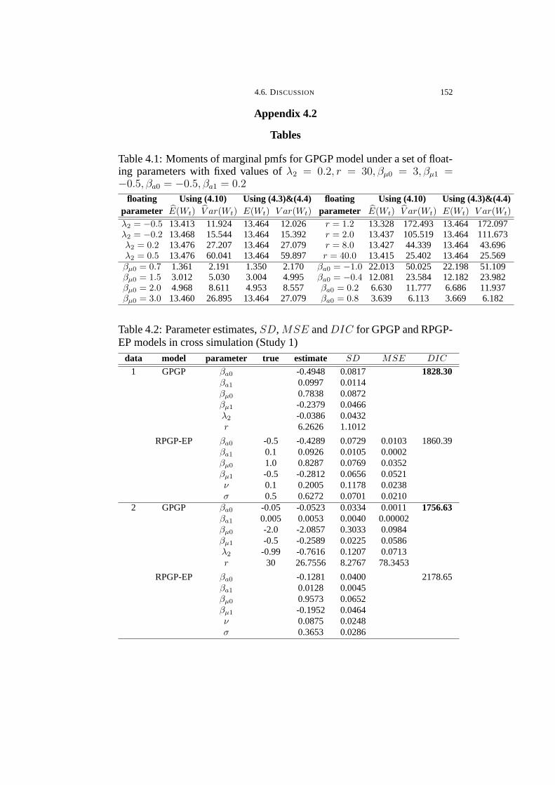
4.6. DISCUSSION 152
Appendix 4.2
Tables
Table 4.1: Moments of marginal pmfs for GPGP model under a set of float-ing parameters with fixed values of λ2 = 0.2, r = 30, βµ0 = 3, βµ1 =−0.5, βa0 = −0.5, βa1 = 0.2
floating Using (4.10) Using (4.3)&(4.4) floating Using (4.10) Using (4.3)&(4.4)parameter E(Wt) V ar(Wt) E(Wt) V ar(Wt) parameter E(Wt) V ar(Wt) E(Wt) V ar(Wt)
λ2 = −0.5 13.413 11.924 13.464 12.026 r = 1.2 13.328 172.493 13.464 172.097λ2 = −0.2 13.468 15.544 13.464 15.392 r = 2.0 13.437 105.519 13.464 111.673λ2 = 0.2 13.476 27.207 13.464 27.079 r = 8.0 13.427 44.339 13.464 43.696λ2 = 0.5 13.476 60.041 13.464 59.897 r = 40.0 13.415 25.402 13.464 25.569βµ0 = 0.7 1.361 2.191 1.350 2.170 βa0 = −1.0 22.013 50.025 22.198 51.109βµ0 = 1.5 3.012 5.030 3.004 4.995 βa0 = −0.4 12.081 23.584 12.182 23.982βµ0 = 2.0 4.968 8.611 4.953 8.557 βa0 = 0.2 6.630 11.777 6.686 11.937βµ0 = 3.0 13.460 26.895 13.464 27.079 βa0 = 0.8 3.639 6.113 3.669 6.182
Table 4.2: Parameter estimates, SD, MSE andDIC for GPGP and RPGP-EP models in cross simulation (Study 1)
data model parameter true estimate SD MSE DIC
1 GPGP βa0 -0.4948 0.0817 1828.30βa1 0.0997 0.0114βµ0 0.7838 0.0872βµ1 -0.2379 0.0466λ2 -0.0386 0.0432r 6.2626 1.1012
RPGP-EP βa0 -0.5 -0.4289 0.0729 0.0103 1860.39βa1 0.1 0.0926 0.0105 0.0002βµ0 1.0 0.8287 0.0769 0.0352βµ1 -0.5 -0.2812 0.0656 0.0521ν 0.1 0.2005 0.1178 0.0238σ 0.5 0.6272 0.0701 0.0210
2 GPGP βa0 -0.05 -0.0523 0.0334 0.0011 1756.63βa1 0.005 0.0053 0.0040 0.00002βµ0 -2.0 -2.0857 0.3033 0.0984βµ1 -0.5 -0.2589 0.0225 0.0586λ2 -0.99 -0.7616 0.1207 0.0713r 30 26.7556 8.2767 78.3453
RPGP-EP βa0 -0.1281 0.0400 2178.65βa1 0.0128 0.0045βµ0 0.9573 0.0652βµ1 -0.1952 0.0464ν 0.0875 0.0248σ 0.3653 0.0286

4.6. DISCUSSION 153
Table 4.3: Mean and variance of the true, GPGP and RPGP-EP models incross simulation (Study 1)
time averagedata model 1 2 3 4 5 6 7 8 over time
1 true mean 2.255 3.104 3.356 3.056 2.278 1.379 0.678 0.279 2.048GPGP 1.966 2.631 2.899 2.605 1.935 1.165 0.578 0.235 1.752
RPGP-EP 2.177 2.739 2.923 2.557 1.900 1.137 0.573 0.243 1.781
true variance 2.731 3.964 4.362 3.924 2.737 1.550 0.719 0.285 2.534GPGP 2.439 3.548 4.032 3.519 2.389 1.307 0.590 0.227 2.256
RPGP-EP 2.861 3.791 4.150 3.495 2.408 1.322 0.620 0.252 2.363
2 true mean 3.262 3.391 3.499 3.571 3.610 3.606 3.566 3.495 3.500GPGP 2.943 3.066 3.168 3.235 3.271 3.265 3.229 3.160 3.167
RPGP-EP 2.430 2.688 2.902 3.055 3.138 3.133 3.058 2.900 2.913
true variance 1.199 1.262 1.315 1.339 1.361 1.361 1.340 1.312 1.311GPGP 1.281 1.352 1.405 1.432 1.456 1.458 1.436 1.403 1.403
RPGP-EP 2.695 3.024 3.289 3.487 3.584 3.579 3.485 3.282 3.303
Table 4.4: Mean and variance of four simulated data sets under differentsituations (Study 2)
time averagedata 1 2 3 4 5 6 7 8 over time
underdispersion mean 2.750 3.088 3.013 3.213 3.300 3.175 3.075 3.075 3.086equidispersion 2.975 3.313 3.238 3.438 3.525 3.400 3.300 3.300 3.311overdispersion 3.125 3.463 3.388 3.588 3.675 3.550 3.450 3.450 3.461zero-inflation 3.025 1.425 0.613 0.238 0.713 0.525 1.350 2.138 1.253
underdispersion variance 1.658 1.777 1.354 1.258 1.428 1.437 1.665 1.412 1.499equidispersion 3.772 3.509 3.120 3.616 3.063 3.585 3.630 2.922 3.402overdispersion 7.402 6.885 6.519 7.410 6.374 7.238 7.162 6.149 6.892zero-inflation 26.860 5.463 2.620 0.639 2.992 1.822 8.306 14.171 7.859

4.6. DISCUSSION 154
Table 4.5: Parameter estimates, SE andDIC in GPGP and RPGP-EP mod-els under different degrees of dispersion (Study 2)
model para- underdispersion equidispersion overdispersion zero-inflation*meter estimate SE estimate SE estimate SE estimate SE
GPGP βa0 -0.0669 0.0194 -0.0389 0.0513 -0.0733 0.0283 1.1370 0.2042βa1 0.0070 0.0024 0.0040 0.0062 0.0080 0.0033 -0.1398 0.0243βµ0 1.1430 0.0368 1.2255 0.0606 1.2365 0.0516 1.1405 0.2459βµ1 -0.2212 0.0312 -0.2037 0.0413 -0.1915 0.0451 -0.0919 0.1932λ2 -0.8792 0.1019 -0.9651 0.0432 -0.9701 0.0422 0.3874 0.0644r 19.3500 8.4734 6.1110 0.4832 4.0845 0.2801 0.3012 0.0397
DIC 1893.60 1943.31 (+2.6%) 1966.24 (+1.2%) 1312.66 NA
RPGP βa0 -0.1809 0.0254 -0.1111 0.0228 -0.1244 0.0368 1.5320 0.1179-EP βa1 0.0188 0.0038 0.0115 0.0032 0.0127 0.0053 -0.1798 0.0162
βµ0 1.0380 0.0064 1.0950 0.0125 1.0880 0.0093 0.6003 0.0220βµ1 -0.4143 0.0157 -0.1672 0.0242 -0.2892 0.0175 -0.6094 0.1260ν 0.1462 0.0731 0.8775 0.1264 1.9810 0.0161 1.9510 0.0344σ 0.1090 0.0059 0.2005 0.0067 0.1189 0.0039 0.6763 0.0679
DIC 2206.33 2435.34 (+10.4%) 2449.17 (+0.6%) 1317.85 NA* A new data set is simulated.
Table 4.6: Parameter estimates, SE and DIC in 2-group GMPGP andRMPGP-EP models for the cannabis data
RMPGP-EP model GMPGP model GMPGP-AR(1) modelgroup parameter estimate SE parameter estimate SE estimate SE
l = 1 βa01 0.0798 0.0304 βa01 0.0455 0.0273 0.0529 0.0268high-level βµ01 2.6200 0.1183 βµ01 2.9600 0.1378 2.4350 0.1433
βµ11 0.0198 0.0022σ1 0.5512 0.0707 λ21 0.7238 0.0260 0.6221 0.0327ν1 1.4060 0.1617 r1 29.600 21.340 25.280 18.840π1 0.4034 0.0812 π1 0.3530 0.0822 0.4694 0.0923
l = 2 βa02 0.1039 0.0287 βa02 0.0915 0.0296 0.0966 0.03272low-level βµ02 1.0750 0.1308 βµ02 1.2910 0.1273 1.084 0.1885
σ2 0.5208 0.0851 λ22 0.1098 0.1581 0.0773 0.1459ν2 1.1640 0.2368 r2 2.7030 2.7870 3.0580 4.2560
DIC 3812.77 DIC 3751.78 3644.21
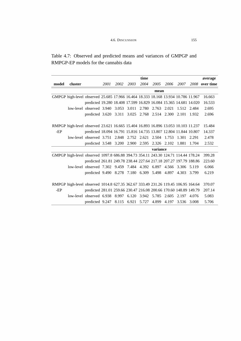
4.6. DISCUSSION 155
Table 4.7: Observed and predicted means and variances of GMPGP and
RMPGP-EP models for the cannabis data
time averagemodel cluster 2001 2002 2003 2004 2005 2006 2007 2008 over time
mean
GMPGP high-level observed 25.685 17.966 16.464 18.333 18.168 13.934 10.786 11.967 16.663
predicted 19.280 18.408 17.599 16.829 16.084 15.365 14.681 14.020 16.533
low-level observed 3.940 3.053 3.011 2.780 2.763 2.021 1.512 2.484 2.695
predicted 3.620 3.311 3.025 2.768 2.514 2.300 2.101 1.932 2.696
RMPGP high-level observed 23.621 16.665 15.404 16.893 16.896 13.053 10.103 11.237 15.484
-EP predicted 18.094 16.791 15.816 14.735 13.807 12.804 11.844 10.807 14.337
low-level observed 3.751 2.848 2.752 2.621 2.504 1.753 1.301 2.291 2.478
predicted 3.548 3.200 2.900 2.595 2.326 2.102 1.881 1.704 2.532
variance
GMPGP high-level observed 1097.8 686.88 394.73 354.11 243.30 124.71 114.44 178.24 399.28
predicted 261.81 249.78 238.44 227.64 217.18 207.27 197.79 188.86 223.60
low-level observed 7.302 9.459 7.484 4.392 6.897 4.566 3.306 5.119 6.066
predicted 9.490 8.278 7.180 6.309 5.498 4.897 4.303 3.799 6.219
RMPGP high-level observed 1014.8 627.35 362.67 333.49 231.26 119.45 106.95 164.64 370.07
-EP predicted 281.01 259.66 230.47 216.08 200.66 170.60 148.89 149.79 207.14
low-level observed 6.938 8.997 6.120 3.942 5.785 2.605 2.197 4.076 5.083
predicted 9.247 8.115 6.921 5.727 4.899 4.197 3.536 3.008 5.706
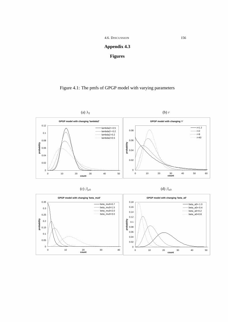
4.6. DISCUSSION 156
Appendix 4.3
Figures
Figure 4.1: The pmfs of GPGP model with varying parameters
(a) λ2
GPGP model with changing 'lambda2'
0
0.02
0.04
0.06
0.08
0.1
0.12
0 10 20 30 40 50count
pro
bab
ility
lambda2=-0.5lambda2=-0.2lambda2=0.2lambda2=0.5
(b) r
GPGP model with changing 'lambda2'
0
0.02
0.04
0.06
0.08
0.1
0.12
0 10 20 30 40 50count
pro
bab
ility
lambda2=-0.5lambda2=-0.2lambda2=0.2lambda2=0.5
GPGP model with changing 'r'
0
0.02
0.04
0.06
0.08
0 10 20 30 40 50 60count
pro
bab
ility
r=1.2r=2r=8r=40
(c) βµ0
GPGP model with changing 'lambda2'
0
0.02
0.04
0.06
0.08
0.1
0.12
0 10 20 30 40 50count
pro
bab
ility
lambda2=-0.5lambda2=-0.2lambda2=0.2lambda2=0.5
GPGP model with changing 'beta_mu0'
0
0.05
0.1
0.15
0.2
0.25
0.3
0.35
0 10 20 30 40count
pro
bab
ility
beta_mu0=0.7beta_mu0=1.5beta_mu0=2.0beta_mu0=3.0
(d) βa0
GPGP model with changing 'lambda2'
0
0.02
0.04
0.06
0.08
0.1
0.12
0 10 20 30 40 50count
pro
bab
ility
lambda2=-0.5lambda2=-0.2lambda2=0.2lambda2=0.5
GPGP model with changing 'beta_a0'
0
0.02
0.04
0.06
0.08
0.1
0.12
0.14
0.16
0.18
0 10 20 30 40 50count
pro
bab
ility
beta_a0=-1.0beta_a0=-0.4beta_a0=0.2beta_a0=0.8
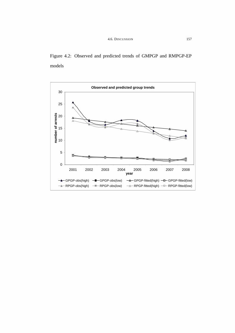
4.6. DISCUSSION 157
Figure 4.2: Observed and predicted trends of GMPGP and RMPGP-EP
models
Observed and predicted group trends
0
5
10
15
20
25
30
2001 2002 2003 2004 2005 2006 2007 2008year
nu
mb
er o
f ar
rest
s
GPGP-obs(high) GPGP-obs(low) GPGP-fitted(high) GPGP-fitted(low)
RPGP-obs(high) RPGP-obs(low) RPGP-fitted(high) RPGP-fitted(low)

4.6. DISCUSSION 158
Figure 4.3: The pmfs of high-level group for GMPGP and RMPGP-EP
models at different t
(a) t = 1
Observed and fitted pmfs of high-level group at t=5
0
0.02
0.04
0.06
0.08
0.1
0.12
0.14
0 10 20 30 40 50 60 70count
pro
bab
ility
GPGP (observed) RPGP-EP (observed) GPGP (fitted) RPGP-EP (fitted)
Observed and fitted pmfs of high-level group at t=1
0
0.05
0.1
0.15
0.2
0 20 40 60 80 100 120 140count
pro
bab
ility
GPGP (observed) RPGP-EP (observed) GPGP (fitted) RPGP-EP (fitted)
(b) t = 5
Observed and fitted pmfs of high-level group at t=5
0
0.02
0.04
0.06
0.08
0.1
0.12
0.14
0 10 20 30 40 50 60 70count
pro
bab
ility
GPGP (observed) RPGP-EP (observed) GPGP (fitted) RPGP-EP (fitted)
Figure 4.4: The pmfs of low-level group for GMPGP and RMPGP-EP mod-
els at different t
(a) t = 1
Observed and fitted pmfs of low-level group at t=5
0
0.05
0.1
0.15
0.2
0.25
0.3
0.35
0 2 4 6 8 10 12 14count
pro
bab
ility
GPGP (observed) RPGP-EP (observed) GPGP (fitted) RPGP-EP (fitted)
Observed and fitted pmfs of low-level group at t=1
0
0.05
0.1
0.15
0.2
0 2 4 6 8 10 12 14count
pro
bab
ility
GPGP (observed) RPGP-EP (observed) GPGP (fitted) RPGP-EP (fitted)
(b) t = 5
Observed and fitted pmfs of high-level group at t=5
0
0.02
0.04
0.06
0.08
0.1
0.12
0.14
0 10 20 30 40 50 60 70count
pro
bab
ility
GPGP (observed) RPGP-EP (observed) GPGP (fitted) RPGP-EP (fitted)
Observed and fitted pmfs of low-level group at t=5
0
0.05
0.1
0.15
0.2
0.25
0.3
0.35
0 2 4 6 8 10 12 14count
pro
bab
ility
GPGP (observed) RPGP-EP (observed) GPGP (fitted) RPGP-EP (fitted)
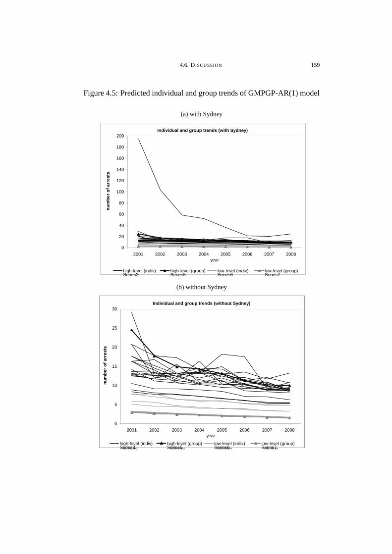
4.6. DISCUSSION 159
Figure 4.5: Predicted individual and group trends of GMPGP-AR(1) model
(a) with Sydney
Individual and group trends (with Sydney)
0
20
40
60
80
100
120
140
160
180
200
2001 2002 2003 2004 2005 2006 2007 2008year
nu
mb
er o
f ar
rest
s
high-level (indiv) high-level (group) low-level (indiv) low-level (group)Series3 Series5 Series6 Series7
(b) without Sydney
Individual and group trends (with Sydney)
0
20
40
60
80
100
120
140
160
180
200
2001 2002 2003 2004 2005 2006 2007 2008year
nu
mb
er o
f ar
rest
s
high-level (indiv) high-level (group) low-level (indiv) low-level (group)Series3 Series5 Series6 Series7
Individual and group trends (without Sydney)
0
5
10
15
20
25
30
2001 2002 2003 2004 2005 2006 2007 2008year
nu
mb
er o
f ar
rest
s
high-level (indiv) high-level (group) low-level (indiv) low-level (group)Series3 Series5 Series6 Series7

CHAPTER 5
Multivariate generalized Poisson log-t geometric process
model
Chapters 2 to 4 extend the PGP models to analyze univariate longi-
tudinal and panel count data with various characteristics (including zero-
inflation, overdispersion and underdispersion while allowing for the serial
correlation and cluster effects). This Chapter extends the generalized Pois-
son geometric process (GPGP) model described in (4.2) described in the
previous Chapter to study multivariate longitudinal count data.
5.1. Background
The modelling of multivariate time series of counts has drawn atten-
tion increasingly as its application ranges widely in different areas. Data
such as sales, crimes, car accidents, occupational injuries, industrial control
and diseases are often measured in a multivariate manner with more than
one outcome associated with the same subject and the outcomes are usually
correlated. Let Wit be the count at time t from the ith time series. The
objective of this Chapter is to innovate an adequate count model for mul-
tivariate longitudinal count data in a geometric process (GP) framework to
address the trend movements, covariate effects, serial correlation between
observations (Wit,Wi,t−L) in individual time series and cross correlation
160

5.1. BACKGROUND 161
(Wit,Wi′,t−L) and contemporaneous correlation (Wit,Wi′t) between time
series where L,L = 1, . . . , n− 1 denotes the lag of the observations.
While the literature for the multivariate distribution is extensive for con-
tinuous data, researches for discrete multivariate counts are relatively lim-
ited due to the computational difficulties in implementation. The multivari-
ate normal distribution is commonly used as an alternative choice to model
discrete data (Karlis, 2003). Unfortunately, it fails particularly when the
count data is skewed due to the prevalence of small or zero observations.
In the multivariate time series of counts, different time series usually
possess different properties such as dispersion, trend movement and serial
correlation between observations. Moreover, cross correlation and contem-
poraneous correlation may exist between pairs of time series. This Chapter
proposes a new model namely multivariate generalized Poisson log-t geo-
metric process (MGPLTGP) model to allow for all these properties. The
model is shown to have several advantages over some existing models in
the literature.
The development of multivariate models starts from the consideration of
cross-sectional count data. Amongst all the available multivariate models,
models with the bivariate Poisson distribution proposed by Kocherlakota
& Kocherlakota (1992) and the multivariate Poisson (MP) distribution by
Johnson et al. (1997) are the most straightforward extensions of the uni-
variate Poisson model. It is because they have closed-form joint probability

5.1. BACKGROUND 162
mass function (pmf). Each random variable of the MP distribution is ex-
pressed as a sum of two independent univariate Poisson random variables
in which one variable is common in all the sums. In this way, the mar-
ginal distribution is essentially the simple Poisson distribution with mean
equals to variance and the covariance between all pairs of variables would
be the mean of the common Poisson variable (Refer to Section 5.2.1 for
more details). However, the equal and positive correlation between all pairs
of Poisson variables is very restrictive and the model is only applicable to
equidispersed data.
Thereafter, Karlis & Meligkotsidou (2005) extended the covariance struc-
ture in the basic MP distribution by allowing a different covariance for each
pair of variables. Nevertheless, the restriction on positive correlation and
equidispersion still remained unsolved. Throughout the past decade, a num-
ber of researches have considered using a mixed model approach to deal
with the overdispersed multivariate counts with negative correlation. A list
of the mixed models can be found in Karlis & Xekalaki (2005). These MP
mixed models can be classified into two types. The first type is generally
a composite of MP distribution with a univariate mixing distribution as it
assumes that the means of the MP random variables are proportional to a
random variable following a univariate mixing distribution. Properties of
this type of models are described in Kocherlakota (1988). Despite that the

5.1. BACKGROUND 163
mixing component adds extra variation to the resultant distribution to ac-
count for data with overdispersion, this model can apply only to positively
correlated multivariate counts as the covariance function is always positive.
As a generalization of the first type, the second type imposes a multi-
variate mixing distribution on the mean vector of the MP distribution. Using
this approach, the covariances of the unconditional MP variables are sim-
ply expressed in terms of the covariances of the mixing parameters. In this
way, the unconditional variables may exhibit negative correlation as well
as overdispersion. Nonetheless, the MP mixed model of the second type,
though is suitable for modelling overdispersed count data with negative cor-
relation, cannot cope with underdispersed data. Moreover, the resulting dis-
tribution is very complicated and in practice most models consider a special
case in which the MP variables are assumed to be independent. See Karlis
& Xekalaki (2005) for more details of the two types of mixed MP distribu-
tions.
In the context of time series analysis, some applications of these afore-
mentioned models include Karlis (2003), Wang et al. (2003) and Lee et al.
(2005). For instances, Karlis (2003) applied the MP model to analyze the
number of road accidents on 24 central roads of Athens during 1987-1991.
In the analysis, the time effect is investigated through the correlation struc-
ture which assumes all pairs of time series have equal and positive corre-
lation. Wang et al. (2003) adopted a bivariate zero-inflated Poisson regres-
sion model to study the monthly musculoskeletal and non-musculoskeletal
5.1. BACKGROUND 164
injuries from November 1992 to October 1995. Their model belongs to the
family of MP mixed models of the second kind and treats time as the expo-
sure without taking into account the serial correlation. Later on, Lee et al.
(2005) extended this model by incorporating multivariate normal random
effects with an autoregressive (AR) structure to account for serial correla-
tion for each individual time series but has not taken into account the cross
correlation between time series. Nonetheless, all these applications have
not addressed the trend movement and are limited to overdispersed data.
To simplify the modelling of covariances between pairs of time series
while allowing for different degrees of dispersion, this Chapter adopts the
approach in the MP mixed model of the second type but replaces the Pois-
son distribution with generalized Poisson distribution (GPD) for the out-
comes to result in a multivariate generalized Poisson mixed model. To
be specific, we extend the generalized Poisson geometric process (GPGP)
model described in Chapter 4 which is so far the most comprehensive model
amongst all existing PGP models to multivariate count data. In essence, this
model with the multivariate mixing distribution not only can allow a flex-
ible degree of dispersion, but also accommodate various contemporaneous
correlation structures by adopting different covariance matrices. Moreover,
as non-stationarity, serial and cross correlation are often prominent in time
series, our proposed model describes the trend movement explicitly while
taking into account the autocorrelation structure in individual time series
and across time series.

5.1. BACKGROUND 165
In our proposed model, assume that the observed multivariate counts
follow independent GPDs, the means of the GPDs after discounting ge-
ometrically (t − 1) times become stationary and form a latent stochastic
process. We then assign the multivariate log-t (MLT) distribution as the
mixing distribution to the latent variables such that its mean and covariance
matrix can accommodate covariate effects and different correlation struc-
tures respectively. The MLT distribution is preferred to multivariate lognor-
mal (MLN) distribution which was adopted by Aitchinson & Ho (1989) and
Ma et al. (2008) as it provides more flexibility in the tail behavior for han-
dling outlying observations. Besides, if appropriate, some serial and cross
correlation structures can be accommodated by incorporating some lagged
observations as time-evolving covariates into the log-linked mean function
in individual time series or across time series. The resultant model is essen-
tially a multivariate version of the RPGP model and GPGP models which
have been investigated in Chapter 3 and 4 respectively.
For model implementation, the MP model and the MP mixed model
adopt the expectation-maximization (EM) algorithm in the likelihood ap-
proach (Karlis, 2003; Karlis & Meligkotsidou, 2007). However such method
becomes computational intensive due to the complexity of the joint pmf as
the number of dimension increases. This shortcoming makes the model less
favorable in real-life applications. On the other hand, Karlis & Xekalaki
(2005) adopted a Bayesian approach for model implementation. In a Bayesian

5.2. A REVIEW OF MULTIVARIATE POISSON MODELS 166
perspective, the evaluation of the complex joint pmf can be avoided by con-
structing a simple Gibbs sampler to simulate the parameters from their full
conditional posterior distributions. Similar to the approach in the RPGP
model, the MLT distribution in our proposed model is expressed in scale
mixtures of MLNs. Under the scale mixtures representation, the parameter
estimation can be simplified by sampling from multivariate normal distri-
bution using Markov chain Monte Carlo (MCMC) algorithms and the addi-
tional mixing parameters in the scale mixtures of MLNs help to identify the
extreme observations in the outlier diagnosis. Refer to Chapter 3 for more
details.
The rest of the Chapter is organized as follows. Section 5.2 will briefly
review the well-established MP models and MP mixed models. Section 5.3
will introduce the proposed multivariate generalized Poisson log-t geomet-
ric process (MGPLTGP) model using scale mixtures of MLNs. In Section
5.4, we will discuss the implementation of MGPLTGP model using MCMC
algorithms followed by the introduction of the model assessment criterion.
After that, a real data analysis of the MGPLTGP model with model com-
parison will be given in Section 5.5. Lastly Section 5.6 will give some
concluding remarks with plausible future extensions.
5.2. A review of multivariate Poisson models
5.2.1. Multivariate Poisson model. The multivariate Poisson (MP) model
is derived through the multivariate reduction (Mardia, 1971). Suppose that
Vi, i = 0, . . . ,m are independent Poisson random variables with mean ηi.

5.2. A REVIEW OF MULTIVARIATE POISSON MODELS 167
Then the random variables Wi = Vi + V0, i = 1, . . . ,m follow jointly a
multivariate Poisson (MP) distribution where m represents the dimension
of the distribution. The joint pmf fMP (w|η) is given by
fMP (w|η) = f(w1, w2, . . . , wm| η0, η1, . . . , ηm)
= exp
(−
m∑
i=0
ηi
)m∏
i=1
ηwi
i
wi!
ξ∑
i=0
m∏
j=1
wj
i
(i!)m−1
η0m∏
k=1
ηk
i
where w = {w1, w2, . . . , wm} and ξ = min(w1, w2, . . . , wm). Marginally,
each Wi follows a Poisson distribution and its mean, variance and covari-
ance are given by
E(Wi) = V ar(Wi) = ηi + η0 and Cov(Wi,Wj) = η0 for all i 6= j.
If η0 = 0, then the joint distribution reduces to a product of m independent
Poisson distributions. However, the use of the MP model is rather restricted
due to the unrealistic assumption that all pairs of variables have the same
covariance. See Johnson et al. (1997) for more details.
To allow a more flexible covariance structure, Karlis & Meligkotsidou
(2005) proposed using a two-way covariance structure to improve the prac-
ticability of the MP model. Assume that Wi =i∑
k=1
Vki +m∑
k=i+1
Vik for
i = 1, . . . ,m − 1 and Wm =m∑
k=1
Vkm, where Vik, i ≤ k ≤ m are inde-
pendent Poisson random variables with mean ηik, then the mean, variance
and covariance become
5.2. A REVIEW OF MULTIVARIATE POISSON MODELS 168
E(Wi) = V ar(Wi) =
i∑k=1
ηki +m∑
k=i+1
ηik, for i < m
m∑k=1
ηkm, for i = m
Cov(Wi,Wj) = ηij, for i < j. (5.1)
In addition, the applicability of the MP model can be enhanced by log-
linking ηik with some covariates such that ln ηik = zTik βik for i ≤ k ≤ m,
where zik = {z0ik, z1ik, . . . , zqikik}T and βik = {β0ik, β1ik, . . . , βqikik}T
are (qik + 1) × 1 vectors of covariates and regression coefficients respec-
tively. Refer to Karlis & Meligkotsidou (2005) for more details. In the
remainder of this Chapter, we will denote by fMP (w|η) the joint pmf
of the MP model with two-way covariance structure and parameter vector
η = {η11, η12, . . . , ηm−1,m, ηmm}T .
Although the extension enables the MP model to accommodate covari-
ate effects and a more flexible covariance structure as it allows varying co-
variances across pairs of (Wi,Wj) in (5.1), clearly the MP model still fails
to fit overdispered or negative correlated data which are commonly found in
real life. Hence, the mixed model approach is considered to remedy these
limitations.
5.2.2. Multivariate Poisson mixed model. A majority of the multi-
variate Poisson mixed models can be classified into two categories. Without
loss of generality, assume that Wi follows a MP distribution with its mean

5.2. A REVIEW OF MULTIVARIATE POISSON MODELS 169
proportional to a univariate random variable α where α has a mixing den-
sity g(α|µ, σ2) with mean µ and variance σ2. The probability function of
the MP mixed distribution can be expressed as
fMPM1(w|µ, σ2) =
∫
α
fMP (w|αη) g(α|µ, σ2) dα.
Examples for the mixing densities include gamma and generalized inverse
Gaussian distributions. The mean, variance and covariance of the first type
of MP mixed model are given by
E(Wi) = Eα[Ew(Wi|αη1i, . . . , αηii, αηi,i+1, . . . , αηim)]
=
Eα
[α(
i∑k=1
ηki +m∑
k=i+1
ηik)
]= µ
(i∑
k=1
ηki +m∑
k=i+1
ηik
), for i < m
Eα
[α(
m∑k=1
ηkm)
]= µ
(m∑
k=1
ηkm
), for i = m
V ar(Wi) = Eα[V arW (Wi|αη1i, . . . , αηii, αηi,i+1, . . . , αηim)] +
V arα[Ew(Wi|αη1i, . . . , αηii, αηi,i+1, . . . , αηim)]
=
µ
(i∑
k=1
ηki +m∑
k=i+1
ηik
)+ σ2
(i∑
k=1
ηki +m∑
k=i+1
ηik
)2
, for i < m
µ
(m∑
k=1
ηkm
)+ σ2
(m∑
k=1
ηkm
)2
, for i = m
Cov(Wi,Wj) = Eα[Covw(Wi,Wj|αη1i, .., αηii, αηi,i+1, .., αηim, αη1j, .., αηjj , αηj,j+1, .., αηjm)]
+Covα[Ew(Wi|αη1i, .., αηii, αηi,i+1, .., αηim)
Ew(Wj|αη1j, .., αηjj , αηj,j+1, .., αηjm)]
= Eα(αηij) + Covα
[α
(i∑
k=1
ηki +m∑
k=i+1
ηik
), α
(j∑
k=1
ηkj +m∑
k=j+1
ηjk
)]
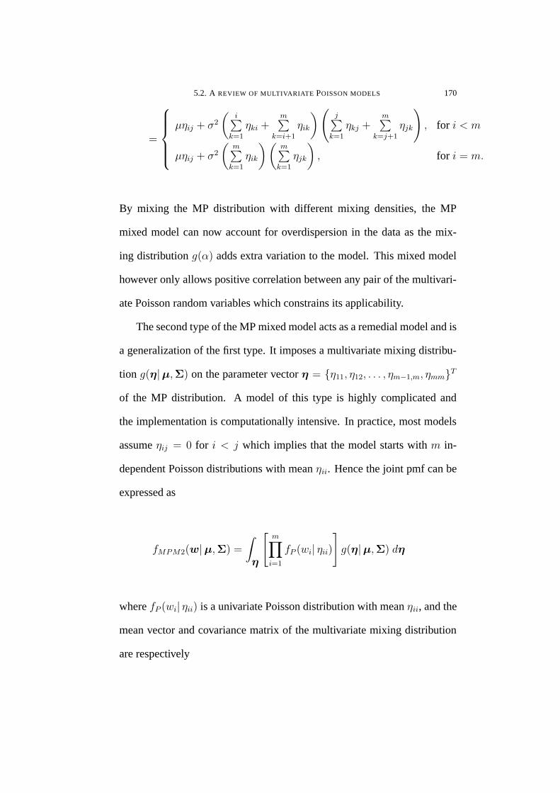
5.2. A REVIEW OF MULTIVARIATE POISSON MODELS 170
=
µηij + σ2
(i∑
k=1
ηki +m∑
k=i+1
ηik
)(j∑
k=1
ηkj +m∑
k=j+1
ηjk
), for i < m
µηij + σ2
(m∑
k=1
ηik
)(m∑
k=1
ηjk
), for i = m.
By mixing the MP distribution with different mixing densities, the MP
mixed model can now account for overdispersion in the data as the mix-
ing distribution g(α) adds extra variation to the model. This mixed model
however only allows positive correlation between any pair of the multivari-
ate Poisson random variables which constrains its applicability.
The second type of the MP mixed model acts as a remedial model and is
a generalization of the first type. It imposes a multivariate mixing distribu-
tion g(η|µ,Σ) on the parameter vector η = {η11, η12, . . . , ηm−1,m, ηmm}T
of the MP distribution. A model of this type is highly complicated and
the implementation is computationally intensive. In practice, most models
assume ηij = 0 for i < j which implies that the model starts with m in-
dependent Poisson distributions with mean ηii. Hence the joint pmf can be
expressed as
fMPM2(w|µ,Σ) =
∫
η
[m∏
i=1
fP (wi| ηii)
]g(η|µ,Σ) dη
where fP (wi| ηii) is a univariate Poisson distribution with mean ηii, and the
mean vector and covariance matrix of the multivariate mixing distribution
are respectively

5.2. A REVIEW OF MULTIVARIATE POISSON MODELS 171
µ =
µ1
µ2
...
µm
and Σ =
σ21 σ12 . . . σ1m
... σ22 . . . σ2m
......
. . ....
σm1 σm2 . . . σ2m
.
Hence, the mean, variance and covariance of the second type of MP mixed
model are written as
E(Wi) = Eη[Ew(Wi| ηii)] = µi
V ar(Wi) = Eη[V arW (Wi| ηii)] + V arη[Ew(Wi| ηii)] = µi + σ2i
Cov(Wi,Wj) = Eη[Covw(Wi,Wj| ηii, ηjj)] + Covη[Ew(Wi| ηii)Ew(Wj| ηjj)]
= Covη(ηii, ηjj) = σij. (5.2)
Explicitly, the covariances of the pairs of multivariate Poisson random vari-
ables are simply the covariances of the mixing distribution, thus this mixed
model of the second type can fit multivariate count data with negative cor-
relation if σij < 0 as well as overdispersion as its variance is greater than its
mean. Amongst all the multivariate mixed distribution, the multivariate log-
normal distribution has been adopted most (Aitchinson & Ho, 1989; Karlis
& Meligkotsidou, 2007; Ma et al., 2008) due to its well-defined moments
and well-established properties. References for the MP mixed models can
be found in Karlis & Xekalaki (2005).
Despite the progressive extensions of the MP mixed models, they still
lack the ability to model underdispersed multivariate count data and so this

5.3. MULTIVARIATE GENERALIZED POISSON LOG-T GEOMETRIC PROCESS MODEL 172
motivates us to replace the Poisson distribution with the generalized Poisson
distribution which can handle both underdispersed and overdispersed data.
Using the MP mixed model approach of the second kind, we pioneer a new
model called multivariate generalized Poisson log-t (MGPLTGP) model
by extending the Poisson distribution to generalized Poisson distribution
(GPD) within the GP modelling framework. In addition, we adopt multi-
variate log-t (MLT) distribution instead of multivariate lognormal (MLN)
distribution in Aitchinson & Ho (1989) as the mixing distribution for the
latent stochastic process (SP) of the GP as the former distribution has an
adjustable heavier-than-normal tail to downweigh the effect of outliers on
the parameter estimation. The MGPLTGP model is introduced in the fol-
lowing Section.
5.3. Multivariate generalized Poisson log-t geometric process model
Previous developments of GP model were confined to univariate data.
In light of the need to study multivariate data which arises in various disci-
plines, we consider a multivariate extension of the PGP model combining
the modelling approach of both GPGP and RPGP models as follows.
5.3.1. Model specification. Denote the vector of counts by W t =
{W1t, . . . ,Wmt}T at time t, t = 1, . . . , n. Assume that Wit follows an
independent GPD with mean Xit, then each Xit =Yit
at−1i
=λ1it
1 − λ2i
, t =
1, . . . , n forms a latent GP where {Yit} is a latent SP and ai is the ratio of
the GP that describes the progression of the trend for Wit. Similar to the

5.3. MULTIVARIATE GENERALIZED POISSON LOG-T GEOMETRIC PROCESS MODEL 173
RPGP model, we further assume that Y ∗t = ln Y t = {Y ∗
1t, . . . , Y∗mt}T fol-
lows a multivariate Student’s t- (MT) distribution fMT (y∗t |µ∗,Σ, ν) with
mean vector and covariance matrix given respectively by
µ =
µ∗1
µ∗2
...
µ∗m
and Σ =
σ21 σ12 . . . σ1m
... σ22 . . . σ2m
......
. . ....
σm1 σm2 . . . σ2m
and degrees of freedom ν. The joint pmf fGPMT
(wt) can be written as
fGPMT
(wt) =
∫
Rm
[m∏
i=1
fGPD(wit|λ1it, λ2i)
]fMT (y∗
t |µ∗,Σ, ν) dy∗t (5.3)
where Rm denotes the set of all real vectors in a m-dimensional space,
fGPD(·|λ1it, λ2i) is the pmf of GPD given by (4.1) with meanλ1it
1 − λ2i
and
varianceλ1it
(1 − λ2i)3, λ1it =
exp(y∗it)(1 − λ2i)
at−1i
and fMT (y∗t |µ∗,Σ, ν) which
acts as the mixing density is given by
fMT (y∗t |µ∗,Σ, ν) =
Γ(ν+m2
)
Γ(ν2)ν
m2 π
m2 |Σ| 12
[1 +
1
ν(y∗
t − µ∗)TΣ
−1(y∗t − µ∗)
]− ν+m2
.(5.4)
The MGPLTGP model examines the trend effect before investigating the
correlation between the pair of time series. Since the resultant MGPLTGP
model does not have a closed-form joint pmf in (5.3), the parameter esti-
mation can be undertaken via MCMC algorithms. Following the idea of the
RPGP in Chapter 3, to enhance the efficiency of the sampling algorithms,
Wakefield et al. (1994) proposed expressing the MT distribution in scale

5.3. MULTIVARIATE GENERALIZED POISSON LOG-T GEOMETRIC PROCESS MODEL 174
mixtures of multivariate normals, so (5.4) becomes:
fMT (y∗t |µ∗,Σ, ν) =
∫ ∞
0
fMN
(y∗
t
∣∣∣∣µ∗,Σ
ut
)fG
(ut
∣∣∣ ν2,ν
2
)dut (5.5)
where fMN
(y∗
t
∣∣∣µ∗, Σut
)is a multivariate normal distribution with mean
vector µ∗ and covariance matrixΣ
ut
, and fG
(ut
∣∣∣ ν2,ν
2
)is a gamma dis-
tribution with mean 1 and variance2
ν. Hence, the joint pmf in (5.3) using
scale mixtures representation in (5.5) is rewritten as
fGPMT
(wt) =
∫
Rm
∫ ∞
0
[m∏
i=1
fGPD(wit|λ1it, λ2i)
]fMN
(y∗
t
∣∣∣∣µ∗,Σ
ut
)fG
(ut
∣∣∣ ν2,ν
2
)dut dy
∗t
where λ1it =exp(y∗it)(1 − λ2i)
at−1it
.
Using scale mixtures representation simplifies the full conditional distri-
butions and thus facilitates the MCMC algorithms such as Gibbs sampling.
Another advantage of using scale mixtures representation is that the result-
ing density contains an extra mixing parameter ut which helps to identify
extreme observations in outlier diagnosis. The smaller the ut, the more
outlying is the vector of observations wt.
5.3.2. Covariate and period effects. To extend the practicability of
the model, we accommodate some time-evolving or exogenous covariate
effects into the mean µ∗i and ratio ai. Denote the covariates by zklit and
regression parameters by βjki, j = µ, a; k = 1, . . . , qj; i = 1, . . . ,m; t =
1, . . . , n for the mean µ∗it and ratio ait functions respectively, where qj, j =

5.3. MULTIVARIATE GENERALIZED POISSON LOG-T GEOMETRIC PROCESS MODEL 175
µ, a represents the number of covariates in µ∗it and ait correspondingly, then
µ∗it = βµ0i + βµ1izµ1it + · · · + βµqµizµqµit (5.6)
ln ait = βa0i + βa1iza1it + · · · + βaqaizaqait. (5.7)
In addition, we assume that there are some piecewise constant time-
varying effects called period effects which change the mean described βjki
and/or the shape of the distribution described by the dispersion parameter
λ2i, covariance matrix Σ and degrees of freedom ν across the intervention
periods. Denote the pth intervention period which starts at Tp and ends at
Tp+1 − 1 by {t, Tp ≤ t ≤ Tp+1 − 1} where P is the total number of periods.
Then
λ2it =P∑
p=1
λ2ip I(Tp ≤ t ≤ Tp+1 − 1) (5.8)
νt =P∑
p=1
νp I(Tp ≤ t ≤ Tp+1 − 1) (5.9)
Σt =P∑
p=1
Σp I(Tp ≤ t ≤ Tp+1 − 1) (5.10)
where I(E) is an indicator function of the event E and λ2ip, νp and
Σp =
σ21p σ12p . . . σ1mp
... σ22p . . . σ2mp
......
. . ....
σm1p σm2p . . . σ2mp
represent the dispersion parameter, degrees of freedom and covariance ma-
trix in period p respectively. Note that period effects can be incorporated in

5.3. MULTIVARIATE GENERALIZED POISSON LOG-T GEOMETRIC PROCESS MODEL 176
the mean µ∗it and ratio ait functions as covariates using indicator variables
and interaction of indicator variables.
Hence, the joint pmf in (5.6) becomes
fGPMT
(wt) =
∫
Rm
∫ ∞
0
[m∏
i=1
fGPD(wit|λ1it, λ2it)
]fMN
(y∗
t
∣∣∣∣µ∗t ,
Σt
ut
)fG
(ut
∣∣∣ νt
2,νt
2
)dut dy
∗t (5.11)
where λ1it =exp(y∗it)(1 − λ2it)
at−1it
and the mean, variance and covariance for
Wit conditional on period p are derived as follows:
E(Wit) = Ex[Ew(Wit|Xit)] = Ex(Xit) =Ey(Yit)
at−1it
=Eu[Ey(Yit|Ut)]
at−1it
=Eu[exp(µ∗
it +σ2
it
2Ut)]
at−1it
=exp(µ∗
it)
at−1it
Eu
[exp
(σ2
it
2Ut
)]
V ar(Wit) = Ex[V arw(Wit|Xit)] + V arx[Ew(Wit|Xit)] =Ey(Yit)
at−1it (1 − λ2it)2
+V ary(Yit)
a2(t−1)it
=exp(µ∗
it)
at−1it (1 − λ2it)2
Eu
[exp
(σ2
it
2Ut
)]+Eu[V ary(Yit|Ut)] + V aru[Ey(Yit|Ut)]
a2(t−1)it
=exp(µ∗
it)
at−1it (1 − λ2it)2
Eu
[exp
(σ2
it
2Ut
)]+Eu
[exp
(2µ∗
it +σ2
it
Ut
)[exp(
σ2it
Ut) − 1]
]
a2(t−1)it
+V aru
[exp
(µ∗
it +σ2
it
2Ut
)]
a2(t−1)it
=exp(µ∗
it)
at−1it (1 − λ2it)2
Eu
[exp
(σ2
it
2Ut
)]
+exp(2µ∗
it)
a2(t−1)it
{Eu
[exp
(2σ2
it
Ut
)]− Eu
[exp
(σ2
it
2Ut
)]2}
Cov(Wit,Wjt) = Covx(Xit, Xjt) =1
(aitajt)t−1Covy(Yit, Yjt)

5.3. MULTIVARIATE GENERALIZED POISSON LOG-T GEOMETRIC PROCESS MODEL 177
=1
(aitajt)t−1
{Eu[Covy(Yit, Yjt|Ut)] + Eu[Eyi
(Yit|Ut)Eyj(Yjt|Ut)]
−Eu[Eyi(Yit|Ut)]Eu[Eyj
(Yjt|Ut)]}
=exp(µ∗
it + µ∗jt)
(aitajt)t−1
{Eu
[exp
(σ2
it + σ2jt
2Ut
)[exp
(σijt
Ut
)− 1]
]
+Eu
[exp
(σ2
it + σ2jt
2Ut
)]− Eu
[exp
(σ2
it
2Ut
)]Eu
[exp
(σ2
jt
2Ut
)]}(5.12)
Although the mean and variance cannot be evaluated explicitly, they can be
approximated using Monte Carlo (MC) integration. By simulating u(j)t , j =
1, . . . ,Ms from fG
(u
(j)t
∣∣∣ νt
2,νt
2
),
E[h(ut)] =
∫ ∞
0
h(ut)fG
(ut
∣∣∣ νt
2,νt
2
)dut
can be evaluated by1
Ms
Ms∑
j=1
h(u(j)t ) where h(ut) is a function of ut and
Ms = 10000 is the number of simulations.
5.3.3. Approximation of joint probability mass function. To study
the distribution in (5.3), we adopt the MC integration discussed below to
approximate the intractable joint pmf. Given the mean vector µ∗t , ratio
function ait, covariance matrix Σt, degrees of freedom νt, and dispersion
parameter λ2it, the joint pmf estimator ft(w) at time t in general, can be
approximated by:
ft(w) =Ms∑
j=1
[m∏
i=1
fGPD
(wi
∣∣∣∣∣exp(y
∗(j)it )(1 − λ2it)
at−1it
, λ2it
)],
wi = 0, . . . ,∞; i = 1, . . . ,m and
y∗(j)t ∼ fMT (y
∗(j)t |µ∗
t ,Σt, νt), j = 1, . . . ,Ms (5.13)

5.3. MULTIVARIATE GENERALIZED POISSON LOG-T GEOMETRIC PROCESS MODEL 178
whereMs = 10000 and the latent vector y∗(j)t = {y∗(j)1t , . . . , y
∗(j)mt }T is simu-
lated from the multivariate Student’s t-distribution in (5.4) given the param-
eters µ∗t , Σt and νt. Then, the marginal mean E(Wit), variance V ar(Wit)
and covariance Cov(Wit) of the approximated joint pmf ft(w) at time t are
obtained by:
E(Wit) =∑
w∈N m0
wift(w), V ar(Wit) =
∑
w∈N m0
w2i ft(w)
− [E(Wit)]
2
and Cov(Wit,Wjt) =
∑
w∈N m0
wiwj ft(w)
− E(Wit)E(Wjt) (5.14)
where Nm0 denotes the set of natural numbers including zero in am-dimensional
space and w = {w1, . . . , wm}T .
To investigate the effects of different parameters on the joint pmf, we
simulated the joint pmf in (5.3) of a bivariate generalized Poisson log-t
geometric process (BGPLTGP) model (m = 2) using MC integration with
Ms = 10000 as described in (5.13). For demonstrative purpose, the period
effect is dropped and thus P = 1. Assuming µ∗it = βµ0i, ln ait = βa0i and
t = 2, we change the values of one of the model parameters each time while
keeping the other parameters constant. The bivariate distributions are dis-
played in the contour plots in Figures 5.1(a) to 5.1(f) in Appendix 5.2 with
contour lines drawn at the same level for fair comparison. Correspond-
ingly, their means, variances, covariances and correlations are summarized
in Table 5.1 in Appendix 5.2. Note that two set of means, variances, and

5.3. MULTIVARIATE GENERALIZED POISSON LOG-T GEOMETRIC PROCESS MODEL 179
covariances using (5.12) and (5.14) are reported to assess the accuracy of
the MC integration.
====================================
Figures 5.1(a) to 5.1(f) and Table 5.1 about here
====================================
The first four contour plots investigate the effect of the parameters in
the mixing density, the multivariate log-t distribution. Starting with Figures
5.1(a) and 5.1(b), σ12 controls solely the covariance and thus the correlation
of the bivariate counts (W1t,W2t) without altering the variances or means
of the bivariate counts. A negative σ12 leads the major axis of the contour
lines to make a negative angle with the vertical axis and a larger magnitude
corresponds to a larger angle between the major axis and the vertical axis
indicating stronger correlation. In other words, the strength of the correla-
tion increases with the magnitude of σ12 while the direction of correlation
aligns with the sign of σ12 as shown in Table 5.1. Meanwhile, σ22 deter-
mines mainly the variance of W2t. The larger the σ22 , the more dispersed is
the count W2t indicated by the more scattered pattern in Figure 5.1(b). As
σ22 has relatively less effects on the mean of W2t and covariance, they only
increase slightly with σ22 .
On the other hand, ν plays a more important role in the variances and
covariance of the bivariate counts but a minor role in the means. The smaller
the ν, the larger are the variances and covariance with a slight increase
in the means. Lastly, Figure 5.1(d) reveals that the parameter βµ02 in the

5.3. MULTIVARIATE GENERALIZED POISSON LOG-T GEOMETRIC PROCESS MODEL 180
mean function µ∗2t of W2t controls its mean, variance and covariance and in
general they all increase with βµ02 as revealed in Table 5.1.
For the parameters in the GPD, βa02 in the ratio function a02 has similar
effect on the distribution as βµ02. This time the smaller the βa02, the larger
are the mean, variance and covariance of W2t. Therefore, Figure 5.1(e)
looks like an inverted mirror image of Figure 5.1(d). Whereas, another dis-
persion parameter λ22 in the GPD mainly controls the degree of dispersion
of W2t without altering much its mean and covariance as illustrated in Fig-
ure 5.1(f). Note that a negative λ22 does not necessarily reveal that W2t is
underdispersed. For example, in the first row the last section of Table 5.1
while W1t is underdispersed when λ21 = −0.8, W2t is overdispersed when
λ22 = −0.8. But in general, the more negative the λ22, the less overdis-
persed is W2t.
Overall the performance of the MC integration is satisfactory as in-
dicated by the close affinity of the approximated mean, variance and co-
variance using (5.12) and (5.14). To minimize the computational time, we
therefore will adapt (5.12) in the sequel to estimate the three moments for
the MGPLTGP model.
5.3.4. Test for serial and cross correlations. The above Sections have
discussed how the MGPLTGP model can accommodate time-evolving co-
variate effects, trend movements, different degrees of dispersion for each

5.3. MULTIVARIATE GENERALIZED POISSON LOG-T GEOMETRIC PROCESS MODEL 181
time series and the contemporaneous correlation between pair of time se-
ries. To achieve an adequate model, any serial correlation between the ob-
servations in each time series and cross correlation between time series need
to be taken into account. For detecting the presence of serial correlation in
each time series {Wit} or cross correlation between two time seriesWit and
Wjt, we first compute the remaining unexplained variation known as the
Pearson’s residual εit, i = 1, . . . ,m; t = 1, . . . , n using
εit =wit − E(Wit)√V ar(Wit)
.
Then, the test statistic TijL under the null hypothesis that the Pearson resid-
uals are not autocorrelated (i = j) or cross-correlated (i 6= j) up to lag L is
given by
TijL = nL∑
k=1
n∑t=k+1
εitεj,t−k
n∑t=1
ε2it
2
and is asymptotically distributed as chi-square χ2(L) with degrees of free-
dom L. See Cameron & Trivedi (1998) for more details.
For the test of serial correlation in each time series Wit, t = 1, . . . , n,
if the p-values are significant up to lag L, an AR(L) structure will be intro-
duced by adding L lagged observations (Wi,t−1, . . . ,Wi,t−L) into the mean
function µ∗it in (5.6). Whereas, for cross correlation between a pair of time
series, L lagged observations (Wi,t−1, . . . ,Wi,t−L) of time series Wit will
be incorporated into the mean function µ∗jt of time series Wjt, t = 1, . . . , n.
Afterwards the model will be refitted and an appropriate AR structure is

5.4. BAYESIAN INFERENCE 182
selected if the resultant model has the smallest DIC with statistically sig-
nificant AR coefficients.
In the next Section, the model implementation and assessment will be
described in details.
5.4. Bayesian inference
For statistical inference, maximum likelihood (ML) method via expec-
tation maximization (EM) algorithm is widely adopted in the MP model
(Karlis, 2003; Wang et al., 2003) or MP mixed model (Karlis & Meligkot-
sidou, 2005, 2007). Despite the pros of using EM algorithm, Karlis &
Meligkotsidou (2005) has pinpointed that as the dimension m of the time
series increases, the computation is more demanding as the complexity of
the model increases. In particular for the MP mixed model, the increasing
number of latent random effects in the mixing distribution will induce a
heavy computational burden and reduce the efficiency of parameter estima-
tion (Karlis & Meligkotsidou, 2007).
To avoid numerical difficulties in maximizing the intractable likelihood
function involving high-dimensional integration, we adopt the Bayesian ap-
proach via Markov chain Monte Carlo (MCMC) algorithms to convert an
optimization problem to a sampling problem. The following Section de-
rives the posterior distribution and univariate full conditional distributions
followed by a discussion of the model assessment measure.

5.4. BAYESIAN INFERENCE 183
5.4.1. MCMC algorithms. Before implementing the MCMC algorithms,
we outline the hierarchical structure of the MGPLTGP model under the
Bayesian framework as follows:
wit ∼ fGPD
(ey∗
it(1 − λ2it)
at−1it
, λ2it
), y∗
t ∼ fMN
(µ∗
t ,Σt
ut
)and ut ∼ fG
(νt
2,νt
2
)
where µit, ait, λ2it, νt and Σt are given by (5.6)-(5.10). In order to construct
the posterior density, some non-informative prior distributions are assigned
to the model parameters as follows:
βjki ∼ N(0, τ 2jki), j = µ, a; k = 0, 1, . . . , qj; i = 1, . . . ,m (5.15)
λ2it ∼ Uniform(−1, 1) (5.16)
Σt ∼ IW (Ψt, rt) (5.17)
νt ∼ Gamma(ct, dt) (5.18)
where
Ψt =P∑
p=1
Ψp I(Tp ≤ t ≤ Tp+1 − 1), rt =P∑
p=1
rp I(Tp ≤ t ≤ Tp+1 − 1),
ct =P∑
p=1
cp I(Tp ≤ t ≤ Tp+1 − 1), dt =P∑
p=1
dp I(Tp ≤ t ≤ Tp+1 − 1),
τ 2jki, cp, dp are some positive constants, IW (Ψt, rt) represents an inverse
Wishart distribution fIW (·|Ψ, r) with meanΨ
r −m− 1, Ψ is a real-valued
positive-definite matrix and r > m − 1 is the degrees of freedom. Inverse
Wishart distribution is commonly used as a conjugate prior for the sym-
metric and positive-definite m×m covariance matrix Σ of the multivariate

5.4. BAYESIAN INFERENCE 184
normal distribution. Its probability density function fIW (Σ|Ψ, r) is given
by
fIW (Σ|Ψ, r) =|Ψ| r
2 |Σ|− (r+m+1)2 exp
[− tr(ΨΣ−1)
2
]
2rm2 Γm( r
2)
where Γm(·) denotes a multivariate Gamma function with dimension m and
tr(A) is the trace of matrix A.
According to Bayes’ theorem, the posterior density is proportional to
the joint densities of complete data likelihood and prior probability distri-
butions. For the MGPLTGP model, denote w = (wT1t,w
T2t, ...,w
Tmt)
T as
the data vector, y∗ = (y∗1t
T ,y∗2t
T , ...,y∗mt
T )T as the latent vector of the sto-
chastic process and u = (u1, u2, ..., un)T as a vector of mixing parameters,
the complete data likelihood function L(θ) for the observed data w and
missing data {y∗,u} is derived as:
L(θ) =n∏
t=1
{[m∏
i=1
fGPD
(ey∗
it
at−1it
, λ2it
)]fMN
(y∗
t
∣∣∣∣µ∗t ,
Σt
ut
)fG
(ut
∣∣∣ νt
2,νt
2
)}(5.19)
where the vector of model parameters θ = (βµ,βa,λ2,Σ,ν)T where βj =
(βj01, ..., βjqj1, ..., βj0m, ..., βjqjm)T , j = µ, a; k = 0, . . . , qj are parameters
in the mean function in (5.6) and ratio function in (5.7), λ2 = (λ211, λ212, . . . , λ2mP )T ,
Σ = (Σ1, . . . ,Σp)T and ν = (ν1, . . . , νP )T .
Treating y∗it and ut as missing observations, the posterior density of the
MGPLTGP model is derived as:

5.4. BAYESIAN INFERENCE 185
f(θ|w,y∗,u) ∝ L(θ)
[m∏
i=1
∏
j=µ,a
qj∏
k=0
fN(βjki| 0, τ 2jki)
]m∏
i=1
P∏
p=1
fU(λ2ip| − 1, 1)
[P∏
p=1
fIW (Σp|Ψp, rp)fG(νp| cp, dp)
]
where fN(·| c, d) represents a normal distribution with mean c and variance
d, fU(·| c, d) is a uniform distribution on the interval [c, d], the complete
data likelihood L(θ) is given by (5.19) and the priors are given by (5.15)-
(5.18).
Knowing the joint posterior density, we can then formulate the set of
conditional posterior densities for all the unknown model parameters which
is essential for Gibbs sampling. The following shows the full conditional
posterior densities for each of the model parameters in θ = (βµ,βa,λ2,Σ,ν)T
and the two sets of missing observations y∗it and ut:
f(βµki|w,y∗,u,β−,λ2,Σ,ν) ∝n∏
t=1
exp
[−(y∗
t − µ∗t )
TΣ
−1t (y∗
t − µ∗t )
2ut
]exp
(−β2
µki
2τ 2µki
)
f(βaki|w,y∗,u,β−,λ2,Σ,ν) ∝n∏
t=1
{[exp(y∗it)(1 − λ2it)
at−1it
+ λ2itwit
]wit−1
exp
[−exp(y∗it)(1 − λ2it)
at−1it
− βakizakit(t− 1)
]}exp
(− β2
aki
2τ 2aki
)
restricted to at−1it < −exp(y∗it)(1 − λ2it)
sitλ2it
if λ2it < 0
f(λ2ip|w,y∗,u,β,λ−2 ,Σ,ν) ∝
n∏
t=1
{(1 − λ2it)
[exp(y∗it)(1 − λ2it)
at−1it
+ λ2itwit
]wit−1
exp
[−exp(y∗it)(1 − λ2it)
at−1it
− λ2itwit
]}
5.4. BAYESIAN INFERENCE 186
restricted to
[1 − sita
t−1it
exp(y∗it)
]−1
< λ2it < 1
f(Σp|w,y∗,u,β,λ2,Σ−,ν) ∝
n∏
t=1
exp
[−(y∗
t − µ∗t )
TΣ
−1t (y∗
t − µ∗t )
2ut
]|Σp|−
rp+m+2
2 exp
[−
tr(Ψp Σ−1p )
2
]
f(νp |w,y∗,u,β,λ2,Σ,ν−) ∝
n∏
t=1
m∏
i=1
ννt2
+ct−1t
(ut
2
) νt2 exp
(−utνt
2− dtνt
)
Γ(
νt
2
)
f(y∗t |w,u,β,λ2,Σ,ν) ∝
m∏
i=1
{[exp(y∗it)(1 − λ2it)
at−1it
+ λ2itwit
]wit−1
exp
[y∗it −
exp(y∗it)(1 − λ2it)
at−1it
]}
exp
[−(y∗
t − µ∗t )
TΣ
−1t (y∗
t − µ∗t )
2ut
]
restricted to y∗it > ln
(−sitλ2ita
t−1it
1 − λ2it
)if λ2it < 0
f(ut|w,y∗,u−,β,λ2,Σ,ν) ∝ exp
[−(y∗
t − µ∗t )
TΣ
−1t (y∗
t − µ∗t )
2ut
]u
νt−12
t exp(−νtut
2
)
where u−,β−,λ−2 ,Σ
− and ν− are vectors of u,β,λ2,Σ and ν excluding
ut, βjki, λ2ip,Σp and νp respectively. The MCMC algorithms are imple-
mented using WinBUGS where the sampling scheme based on the condi-
tional posterior densities is outlined in this Section and the Gibbs sampling
procedures are described in Section 1.4.3.
5.4.2. Model selection criterion. Under the Bayesian approach, we
adopt a model comparison criterion namely the deviance information cri-
terion (DIC) originated by Spiegelhalter et al. (2002) which measures the
fit of the data to the model and at the same time account for the model
complexity. DIC is defined as the sum of a classical measure of fit called
5.5. REAL DATA ANALYSIS 187
posterior mean devianceD(θ) and twice the effective number of parameters
pD which accounts for the model complexity.
For the MGPLTGP model, the DIC output by WinBUGS is defined as
DIC = D(θ) + pD
= − 4
M
M∑
j=1
n∑
t=1
m∑
i=1
ln
[fGPD
(wit
∣∣∣∣∣exp(y∗it
(j))(1 − λ(j)2it)
a(j)(t−1)it
, λ(j)2it
)]
+2n∑
t=1
m∑
i=1
ln
[fGPD
(wit
∣∣∣∣exp(y∗it)(1 − λ2it)
at−1it
, λ2it
)]
where M is the number of realizations in the MCMC sampling algorithms,
θ(j) and y∗it(j) represent the jth posterior sample of parameter θ and y∗it re-
spectively, and θ and y∗it are their posterior means. Model with a smaller
DIC is chosen as the best model since it has a better fit to the data after
accounting for the model complexity.
5.5. Real data Analysis
The practicability of our proposed MGPLTGP model is demonstrated
through the study of the use of amphetamine and narcotics in New South
Wales (NSW), Australia. The overview, data structure, model fitting proce-
dures and lastly the results are discussed as follows.
5.5.1. Overview. Amphetamine is a psychostimulant drug that causes
euphoria and decreased fatigue. An abusive use of this illicit drug makes
user experience drug-induced psychosis which may lead to aggressive and
violent behaviour (McKetin et al., 2006). In the past decade, the prevalence
of amphetamine type substances use in Australia stabilized during 1998 to

5.5. REAL DATA ANALYSIS 188
2002 after a substantial rise from 1993 to 1998, but has flared up again in
late 2002 to 2007 as revealed by the figure that the emergency department
admissions of amphetamine type substances use surged by 139% in NSW.
This upsurge is believed to be caused by the heroin shortage in Australia
which started at around late December in 2000 and prompted many heroin
users to switch to amphetamine use (Weatherburn et al., 2003). Elaborately,
heroin shortage was the consequence of the dismantling of a major syndi-
cate in mid-2000 which allegedly had been bringing in large shipments of
heroin to Australia from traditional source countries on a very regular basis.
Thereafter, the increasing risk in smuggling heroin into Australia together
with more active street-level drug law enforcement led to the dramatic fall
in heroin availability and drug purity and subsequently the mounting heroin
price and difficulty in obtain heroin (Degenhardt et al., 2005). Vividly the
reduction in heroin use is ongoing after the onset of heroin shortage, how-
ever whether it is associated to an increase in amphetamine substance use
remains debatable.
Treating use or possession of amphetamine and narcotics as a proxy
of amphetamine type substances use and heroin use respectively in NSW,
Snowball et al. (2008) examined the relationship between the monthly num-
ber of arrests for use or possession of the two illicit drugs during 1995 to
2008 using a tradition multivariate time series model and found no evi-
dence to support the association between heroin shortage and increasing
amphetamine type substances consumption. Their model has allowed for

5.5. REAL DATA ANALYSIS 189
the non-stationarity of the two time series yet does not have an explicit
trend component to investigate the trend movement. To obtain a more clear
picture on how heroin shortage affects the trend movement and detect any
serial, contemporaneous and cross correlations in the arrests for use or pos-
session of amphetamines and narcotics, we fitted a bivariate generalized
Poisson log-t geometric process (BGPLTGP) model (m = 2) to the data
described below.
5.5.2. Data and model fitting. The data in Appendix 5.1 consists of a
bivariate time series on the monthly number of arrests for use or possession
of amphetamine (W1t) and narcotics (W2t) in Sydney, one of the 153 local
government areas (LGAs) in NSW from January 1995 to December 2008
(n = 168) and can be assessed on the official website of the NSW Bureau of
Crime Statistics and Research (the link is given at the end of Section 4.5.1).
Instead of using an aggregate number of arrests in a state level, we focus
on the data from Sydney, one of the 153 LGAs in NSW because its trend
pattern does not differ much from that of the aggregate data in the state level
used in Snowball et al. (2008) as Sydney is the metropolis of NSW with the
highest arrest rates of illicit drug use or possession. The bivariate time series
of monthly number of arrests are plotted in Figure 5.2 in Appendix 5.3 with
a vertical reference line indicating the onset of heroin shortage.
====================================
Figure 5.2 about here
====================================

5.5. REAL DATA ANALYSIS 190
In Figure 5.2, the numbers of arrests for use or possession of both drugs
show an upward trend collectively before heroin shortage with the arrests
for narcotics use outnumber that for amphetamine. Noticeably once heroin
shortage began in late December 2000 (t = 72), the trend for narcotics lev-
els off gradually with less variation while that for amphetamine continues
to grow with inflating overdispersion. Besides, there are abrupt changes
in the means of both time series after heroin shortage commenced. The
mean monthly number of arrests surges from 9.31 cases to 24.98 cases for
amphetamine use or possession while that of narcotics slumps from 21.58
cases to 15.28 cases. In addition, the contemporaneous correlation between
the bivariate time series is although insignificant (rw = −0.09, p = 0.243),
the contemporaneous correlation in different periods are significantly pos-
itive (rw1 = 0.370, p = 0.0007; rw2 = 0.269, p = 0.004) with a higher
correlation rw1 prior to heroin shortage.
Taking into account the trend movement in each time series and contem-
poraneous correlations between time series before and during heroin short-
age, we fitted a BGPLTGP model to investigate whether heroin shortage
exacerbates amphetamine use contemporaneously in Sydney. Since heroin
shortage is expected to incur a change in the mean, trend movement and
contemporaneous correlation structure of the bivariate time series, we de-
fine the time before shortage as the control period (p = 1, T1 = 1) and those
months after December 2000 as the intervention period (p = 2, T2 = 73)
and incorporate period effects into the dispersion parameter λ2t, degrees

5.5. REAL DATA ANALYSIS 191
of freedom νt and covariance matrix Σt to allow varying contemporaneous
correlation structures and degrees of dispersion in different periods. In ad-
dition, we incorporate the period effect as covariate effect zµ1it = za2it =
b = 0, 1 in the mean function in (5.6) and ratio function in (5.7) to detect
any changes in the mean or trend of the monthly number of arrests for use
or possession of the two illicit drugs due to heroin shortage. Furthermore,
since non-monotone trend is observed in Figure 5.2, we accommodate the
natural logarithm of time t as the time-evolving covariate (za1it = ln t) and
an interaction term of time and heroin shortage (za3it = b ln t = 0, ln t)
in the ratio function to allow a change in trend movement across time and
period. In other words, the mean function µ∗it, ratio function ait, disper-
sion parameter λ2it in (5.8), degrees of freedom νt in (5.9) and covariance
matrices Σt in (5.10) for i = 1, 2 and t = 1, . . . , 168 are expressed as
µ∗it = βµ0i + βµ1ib (5.20)
ln ait = βa0i + βa11 ln t+ βa2ib+ βa3ib ln t (5.21)
λ2it = λ2i1 I(1 ≤ t ≤ 72) + λ2i2 I(73 ≤ t ≤ 168)
νt = ν1 I(1 ≤ t ≤ 72) + ν2 I(73 ≤ t ≤ 168)
Σt = Σ1 I(1 ≤ t ≤ 72) + Σ2 I(73 ≤ t ≤ 168) (5.22)
Using the MCMC algorithms described in Section 5.4.1, we use non-
informative priors by setting τ 2jki = 1000 in (5.15), Ψ1 = Ψ2 =
0.1 0.005
0.005 0.1
,

5.5. REAL DATA ANALYSIS 192
r1 = r2 = 2 in (5.17) and c1 = c2 = d1 = d2 = 0.01 in (5.18). After imple-
menting the MCMC algorithms using WinBUGS, the parameter estimates
are given by the posterior medians of the samples.
To assess the competency of our proposed model, two competitive mod-
els are considered for model comparison. The first one is the bivariate Pois-
son (BP) model with two-way covariance structure described in Section
5.2.1 with Wit = Viit + V12t, i = 1, 2. The mean ηiit of Viit in (5.1) is
log-linked to the same set of covariates as in the BGPLTGP model such that
ln ηiit = β0ii + β1iib+ β2ii ln t+ β3ii(ln t)2 + β4iib ln t+ β5iib(ln t)
2
where i = 1, 2 refers to amphetamine and narcotics respectively and b =
0, 1 indicates the presence of heroin shortage. Besides, the contemporane-
ous correlation η12t between the bivariate time series in (5.1) which is given
by
ln η12t = β012 + β112b (5.23)
detects any change in the contemporaneous correlation structures.
Another competitive model is the bivariate Poisson mixed model of the
second type mentioned in Section 5.2.2. In particular we adopt a multivari-
ate log-normal distribution as the mixing density suggested by Aitchinson
& Ho (1989) and the resultant model is named as BPLN model. In this
model, the log-linked mean function µit in (5.2) is given by
lnµit = β0i + β1ib+ β2i ln t+ β3i(ln t)2 + β4ib ln t+ β5ib(ln t)
2 (5.24)
5.5. REAL DATA ANALYSIS 193
and a period effect is incorporated into the covariance matrix Σt in the
same way as (5.22) in the BGPLTGP model to allow for different contem-
poraneous correlation structures between the bivariate time series in differ-
ent periods. The BP and BPLN models are considered as competitive be-
cause they incorporate the same exogenous effect b, similar time-evolving
covariates ln t and (ln t)2 and their interactions b ln t and b(ln t)2 to allow
for non-linear trend patterns in both time series. These assimilate with the
time-evolving covariates in the ratio function ait in (5.21) of the BGPLTGP
model in which ln at−1it = (t− 1) ln ait = (t− 1)(βa0i + βa1i ln t+ βa2ib+
βa3ib ln t) where βaki, k = 0, . . . , 3 can allow for a variety of trend patterns
similar to βkii and βki, l = 2, . . . , 5 in (5.23) and (5.24) for the BP and
BPLN models respectively.
Last but not least, we fitted a bivariate Poisson lognormal geometric
process (BGPLNGP) model using bivariate lognormal distribution with the
same mean and ratio functions as in the BGPLTGP model except that the
bivariate Student’s t-distribution is replaced by the bivariate normal distri-
bution with the same covariance matrix Σt given by (5.22) for y∗t .
Overall, the four models assume Poisson distribution, Poisson distribu-
tion mixed with bivariate lognormal distribution, Poisson GP mixed with
bivariate lognormal distribution and generalized Poisson GP mixed with bi-
variate log-t distribution for the bivariate time series, namely the BP, BPLN,

5.5. REAL DATA ANALYSIS 194
BPLNGP and BGPLTGP models. All models have allowed for heroin short-
age effect in the means, non-monotone trends and contemporaneous corre-
lation but in different ways due to different model structures and data distri-
butions. The first three models are compared to the BGPLTGP model to in-
vestigate whether the GP approach versus the multivariate Poisson or mixed
multivariate Poisson approach as well as whether the bivariate log-t mixing
distribution versus bivariate lognormal distribution are more preferable and
provide better model fit in analyzing multivariate longitudinal count data.
The results of the analysis including parameter estimates, standard errors
(SE) and DIC output in WinBUGS are summarized in the following Sec-
tion.
5.5.3. Results. Table 5.2 in Appendix 5.2 reports the estimate and stan-
dard error (SE) of the parameters for the four fitted models. Using the
parameter estimates, the expected value, variance and covariance of the
monthly number of arrests for the two illicit drugs use or possession over
time are calculated. For the BP and BGPLTGP models, (5.1) and (5.12)
are used respectively. For the BPLN model, the mean, variance and covari-
ance of the lognormal distribution are substituted in (5.2). Whereas for the
BPLNGP model, the expected number, variance and covariance are derived
in a similar way as (5.2) and are given by
E(Wit) =exp(µ∗
it +σ2
it
2)
at−1it
, V ar(Wit) =exp(µ∗
it +σ2
it
2)
at−1it
+exp(2µ∗
it + σ2it)[exp(σ2
it) − 1]
a2(t−1)it

5.5. REAL DATA ANALYSIS 195
and Cov(Wit,Wjt) =exp
(µ∗
it + µ∗jt +
σ2it
2+
σ2jt
2
)[exp(σijt) − 1]
(aitajt)t−1
where µ∗it and ait are defined in (5.20) and (5.21) respectively as in the
BGPLTGP model. To visualize the model performance and facilitate com-
parison, the expected monthly number of arrests for use or possession of
amphetamine and narcotics are illustrated respectively in Figures 5.3(a) and
5.3(b) in Appendix 5.3 for all the models. Similarly, the SE of the monthly
number of arrests for the two illicit drugs use or possession are plotted in
Figures 5.4(a) and 5.4(b) in Appendix 5.3.
===============================================
Table 5.2 and Figures 5.3(a), 5.3(b), 5.4(a) and 5.4(b) about here
===============================================
Figures 5.3(a) and 5.3(b) indicate the consistent increasing trends for
the bivariate time series. After allowing for the trends, the contemporary
correlation between the two time series is still weakly positive but ceases to
be significant both before and during the heroin shortage as shown by the
insignificant covariance parameters (labelled as ‘cov’ in the third column
‘type’ in Table 5.2) in all fitted models (95% credibility intervals include
zero) except for the BP model in Table 5.2. Amongst the four models, BP
model gives the worst fit to the data as it has the largest DIC. The signif-
icant covariance parameters and the largest DIC can be explained by its
inability to account for overdispersion in the bivariate counts as illustrated
in Figures 5.4(a) and 5.4(b) that its SE is substantially lower than the other

5.5. REAL DATA ANALYSIS 196
three models. Due to the ability to account for overdispersion, the BPLN
and BPLNGP models give substantially smaller DICs than the BP model
indicating an improvement in the model fit. Not surprisingly, their DICs
are close since the two models have similar model structures except that the
latter adopts a GP approach. Their expected monthly numbers of arrests and
SEs are also comparable as revealed in Figures 5.3 and 5.4. Nevertheless,
the smaller DIC in the BPLNGP model supports the use of a GP approach
with an explicit ratio function for the trend movement in modelling multi-
variate longitudinal count data.
Although both BPLN and BPLNGP models can account for overdis-
persion, the BGPLTGP model in which the GPD for the data and bivari-
ate log-t distribution for the underlying stochastic process {Y ∗t} provide a
wider range of dispersion, gives the best model fit (smallest DIC in Ta-
ble 5.2) to the data and thus is chosen as the best model. With reference
to Figure 5.3(a) which plots the expected monthly number of arrests for
amphetamine use or possession, the upward trend of the BGPLTGP model
continues throughout the period with a slightly higher rate of increase dur-
ing the period of heroin shortage. On the contrary, as shown in Figure
5.3(b), the expected monthly number of arrests for narcotics use or posses-
sion is higher at the start and rises at a faster rate than that of amphetamine
before heroin shortage. Followed by a rapid drop in the mean, the growth
ceases after the onset of heroin shortage in late December 2000. Besides, as
5.5. REAL DATA ANALYSIS 197
revealed in Figures 5.4(a) and 5.4(b), the SE of the monthly number of ar-
rests for amphetamine use or possession inflates with the mean throughout
the entire period. On the other hand, the monthly number of arrests for nar-
cotics use or possession becomes less overdispersed with a minor growth in
variance after the onset of heroin shortage.
Lastly, we performed the tests for serial and cross correlations described
in Section 5.3.4 for the best model, the BGPLTGP model. With respect to
serial correlation, no significant serial correlation is found for amphetamine
since the p-values of the chi-square test described in Section 5.3.4 for test-
ing serial correlation up to lag 1,2,3,4 and 5 are 0.411, 0.509, 0.678, 0.416
and 0.555 respectively. However, significant serial correlations are de-
tected for narcotics up to at least lag 5 with p-values equal to 6.36×10⁻⁶,
1.41×10⁻⁸, 5.81×10⁻¹¹, 7.68×10⁻¹³ and 2.49×10⁻¹³ for lag up to 1, 2,
3, 4 and 5 correspondingly. These suggest that adding some lagged ob-
servations (W2,t−1, . . . ,W2,t−5) into the mean function µ∗2t in (5.20) may
help to reduce the serial dependency. For cross correlation, the monthly
number of arrests for amphetamine use or possession has significant cross
correlations (up to lag 6) with that for narcotics use or possession. The
p-values for testing whether Corr(W1t,W2,t−L) are significantly different
from zero are 0.07, 0.04, 0.03, 0.02, 0.03, 0.01, 0.02, 0.10, 0.62, 0.37,
0.57 and 0.19 for L = −7, . . . ,−1, 0, 1, . . . , 4 respectively. To take into
account this long-term association, we incorporated some lagged observa-
tions (W1,t−1, . . . ,W1,t−6) from amphetamine into the mean function µ∗2t

5.5. REAL DATA ANALYSIS 198
for narcotics and vice versa. Different AR structures were fitted and the fi-
nal BGPLTGP model with the smallest DIC (1991.23) and significant AR
terms is achieved with the mean functions for the bivariate time series given
by
µ∗1t = 1.908 + 1.692b+ 0.0106w2,t−1
µ∗2t = 2.2 + 0.651b+ 0.0142w2,t−1 + 0.01w2,t−2.
where all βµk1, k = 0, 1, 2 and βµk2, k = 0, . . . , 3 in the mean functions are
significant. Besides, all other model parameters are quantitatively similar to
that of the BGPLTGP model without accounting for serial and cross corre-
lations given in the last column of Table 5.2. The parameter estimates, SE
and DIC of the final model are given in Table 5.3 in Appendix 5.2.
====================================
Table 5.3 about here
====================================
Regarding the objective of the study, the insignificant covariance pa-
rameters σ12p, p = 1, 2 in the final model reveal that the weak positive
contemporaneous correlation across the bivariate time series does not give
any evidence of the instantaneous association between the growth in the
monthly number of arrests for amphetamine use or possession and the de-
cline in the monthly number of arrests for narcotics use or possession due to
heroin shortage in Sydney. Unexpectedly, concerning the long-term associ-
ation, the significant parameter βµ21 = 0.0106 in the final model (95% CI
5.6. DISCUSSION 199
for βµ21:[0.0015, 0.0191]) implies that after the trend movements have been
accounted for, an increase in the number of arrests for use or possession
of narcotics in a certain month is followed by an increase in the number of
arrests for use or possession of amphetamine in the next month (lag 1). Our
finding, though confined to Sydney LGA, on one hand agrees with Snowball
et al. (2008) that the decline in the monthly number of arrests for narcotics
use or possession is not accompanied by the growth in the monthly num-
ber of arrests for amphetamine use or possession at a state level for all 153
LGAs in NSW. On the other hand, another finding that the growth of the
number of arrests for narcotics use or possession in the previous month is
positively associated with the current growth of that for amphetamine dis-
agrees with Snowball et al. (2008) which found no long-term association
between the monthly numbers of arrests for narcotics and amphetamine use
or possession.
5.6. Discussion
In this Chapter, we propose the multivariate generalized Poisson log-t
geometric process (MGPLTGP) model which is essentially a generalized
Poisson mixed model using multivariate log-t distribution as the mixing
density in the GP modelling framework. The model has several outstanding
properties over some traditional multivariate Poisson count models. First, it
can handle negatively correlated multivariate counts which the multivariate

5.6. DISCUSSION 200
Poisson (MP) models fail to do so. Secondly, it fits multivariate longitudi-
nal count data with different degree of dispersion ranging from overdisper-
sion to underdispersion which is a shortcoming of the MP mixed models.
Thirdly, the trend movement is analyzed explicitly using a ratio function
that ‘detrends’ the latent GP {Xit, t = 1, . . . , n} geometrically to a station-
ary stochastic process {Yit} which is then fitted by a mixing distribution.
Lastly, the mixing density, the multivariate log-t distribution has a heavier-
than-lognormal tail which can handle serious overdispersion due to outlying
observations.
The model is implemented through MCMC sampling algorithms using
WinBUGS. By expressing the multivariate log-t distribution in scale mix-
tures of multivariate lognormals, the MCMC algorithms are facilitated since
the full conditional distributions of the model parameters are simplified and
the mixing parameters enable outlier diagnosis. The practicability of the
model is demonstrated through the analysis of a bivariate time series of the
monthly number of arrests for two illicit drugs use or possession in Sydney.
Results in Section 5.5.3 indicate that our proposed model gives the best
model fit (smallest DIC) and is more preferable to other three competitive
models including the bivariate Poisson model, bivariate Poisson lognormal
model and bivariate Poisson lognormal geometric process model because
of its nicer properties.
Last but not least, concerning the need in examining the cluster effects
which are often observed in multivariate panel count data, the proposed

5.6. DISCUSSION 201
model can be easily extended to incorporate mixture effects and random
effects to allow for heterogeneity in the multiple time series. We believe that
the extended mixture model, which can identify subgroups of multivariate
time series comprising the population, would be worthy of future research.
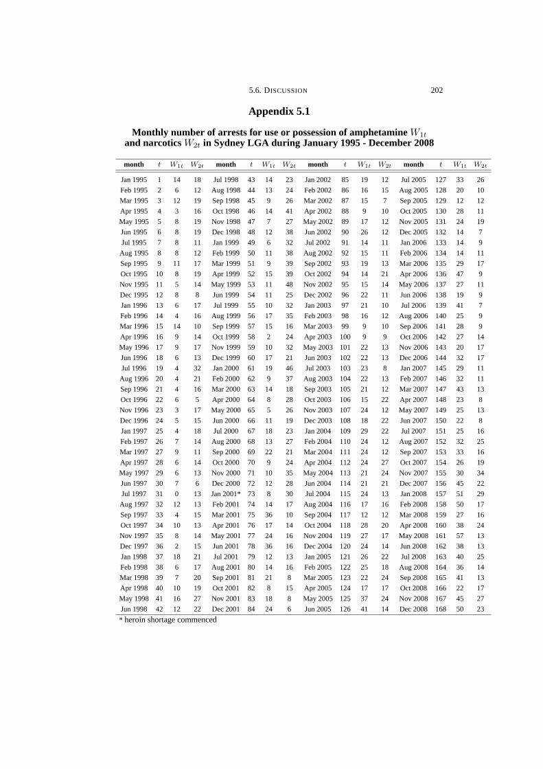
5.6. DISCUSSION 202
Appendix 5.1
Monthly number of arrests for use or possession of amphetamine W1tand narcotics W2t in Sydney LGA during January 1995 - December 2008
month t W1t W2t month t W1t W2t month t W1t W2t month t W1t W2t
Jan 1995 1 14 18 Jul 1998 43 14 23 Jan 2002 85 19 12 Jul 2005 127 33 26
Feb 1995 2 6 12 Aug 1998 44 13 24 Feb 2002 86 16 15 Aug 2005 128 20 10
Mar 1995 3 12 19 Sep 1998 45 9 26 Mar 2002 87 15 7 Sep 2005 129 12 12
Apr 1995 4 3 16 Oct 1998 46 14 41 Apr 2002 88 9 10 Oct 2005 130 28 11
May 1995 5 8 19 Nov 1998 47 7 27 May 2002 89 17 12 Nov 2005 131 24 19
Jun 1995 6 8 19 Dec 1998 48 12 38 Jun 2002 90 26 12 Dec 2005 132 14 7
Jul 1995 7 8 11 Jan 1999 49 6 32 Jul 2002 91 14 11 Jan 2006 133 14 9
Aug 1995 8 8 12 Feb 1999 50 11 38 Aug 2002 92 15 11 Feb 2006 134 14 11
Sep 1995 9 11 17 Mar 1999 51 9 39 Sep 2002 93 19 13 Mar 2006 135 29 17
Oct 1995 10 8 19 Apr 1999 52 15 39 Oct 2002 94 14 21 Apr 2006 136 47 9
Nov 1995 11 5 14 May 1999 53 11 48 Nov 2002 95 15 14 May 2006 137 27 11
Dec 1995 12 8 8 Jun 1999 54 11 25 Dec 2002 96 22 11 Jun 2006 138 19 9
Jan 1996 13 6 17 Jul 1999 55 10 32 Jan 2003 97 21 10 Jul 2006 139 41 7
Feb 1996 14 4 16 Aug 1999 56 17 35 Feb 2003 98 16 12 Aug 2006 140 25 9
Mar 1996 15 14 10 Sep 1999 57 15 16 Mar 2003 99 9 10 Sep 2006 141 28 9
Apr 1996 16 9 14 Oct 1999 58 2 24 Apr 2003 100 9 9 Oct 2006 142 27 14
May 1996 17 9 17 Nov 1999 59 10 32 May 2003 101 22 13 Nov 2006 143 20 17
Jun 1996 18 6 13 Dec 1999 60 17 21 Jun 2003 102 22 13 Dec 2006 144 32 17
Jul 1996 19 4 32 Jan 2000 61 19 46 Jul 2003 103 23 8 Jan 2007 145 29 11
Aug 1996 20 4 21 Feb 2000 62 9 37 Aug 2003 104 22 13 Feb 2007 146 32 11
Sep 1996 21 4 16 Mar 2000 63 14 18 Sep 2003 105 21 12 Mar 2007 147 43 13
Oct 1996 22 6 5 Apr 2000 64 8 28 Oct 2003 106 15 22 Apr 2007 148 23 8
Nov 1996 23 3 17 May 2000 65 5 26 Nov 2003 107 24 12 May 2007 149 25 13
Dec 1996 24 5 15 Jun 2000 66 11 19 Dec 2003 108 18 22 Jun 2007 150 22 8
Jan 1997 25 4 18 Jul 2000 67 18 23 Jan 2004 109 29 22 Jul 2007 151 25 16
Feb 1997 26 7 14 Aug 2000 68 13 27 Feb 2004 110 24 12 Aug 2007 152 32 25
Mar 1997 27 9 11 Sep 2000 69 22 21 Mar 2004 111 24 12 Sep 2007 153 33 16
Apr 1997 28 6 14 Oct 2000 70 9 24 Apr 2004 112 24 27 Oct 2007 154 26 19
May 1997 29 6 13 Nov 2000 71 10 35 May 2004 113 21 24 Nov 2007 155 30 34
Jun 1997 30 7 6 Dec 2000 72 12 28 Jun 2004 114 21 21 Dec 2007 156 45 22
Jul 1997 31 0 13 Jan 2001* 73 8 30 Jul 2004 115 24 13 Jan 2008 157 51 29
Aug 1997 32 12 13 Feb 2001 74 14 17 Aug 2004 116 17 16 Feb 2008 158 50 17
Sep 1997 33 4 15 Mar 2001 75 36 10 Sep 2004 117 12 12 Mar 2008 159 27 16
Oct 1997 34 10 13 Apr 2001 76 17 14 Oct 2004 118 28 20 Apr 2008 160 38 24
Nov 1997 35 8 14 May 2001 77 24 16 Nov 2004 119 27 17 May 2008 161 57 13
Dec 1997 36 2 15 Jun 2001 78 36 16 Dec 2004 120 24 14 Jun 2008 162 38 13
Jan 1998 37 18 21 Jul 2001 79 12 13 Jan 2005 121 26 22 Jul 2008 163 40 25
Feb 1998 38 6 17 Aug 2001 80 14 16 Feb 2005 122 25 18 Aug 2008 164 36 14
Mar 1998 39 7 20 Sep 2001 81 21 8 Mar 2005 123 22 24 Sep 2008 165 41 13
Apr 1998 40 10 19 Oct 2001 82 8 15 Apr 2005 124 17 17 Oct 2008 166 22 17
May 1998 41 16 27 Nov 2001 83 18 8 May 2005 125 37 24 Nov 2008 167 45 27
Jun 1998 42 12 22 Dec 2001 84 24 6 Jun 2005 126 41 14 Dec 2008 168 50 23
* heroin shortage commenced
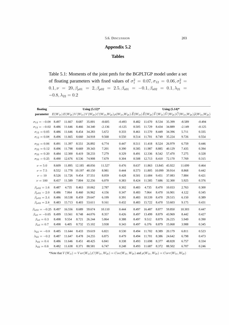
5.6. DISCUSSION 203
Appendix 5.2
Tables
Table 5.1: Moments of the joint pmfs for the BGPLTGP model under a set
of floating parameters with fixed values of σ21 = 0.07, σ12 = 0.06, σ2
2 =
0.1, ν = 20, βµ01 = 2, βµ02 = 2.5, βa01 = −0.1, βa02 = 0.1, λ21 =
−0.8, λ22 = 0.2
floating Using (5.12)* Using (5.14)*
parameter E(W1t)E(W2t)V (W1t)V (W2t)C(W1t,W2t)ρ(W1t,W2t) bE(W1t) bE(W2t) bV (W1t) bV (W2t) bC(W1t,W2t)bρ(W1t,W2t)
σ12 = −0.08 8.497 11.667 8.687 35.001 -8.605 -0.493 8.482 11.670 8.534 35.399 -8.589 -0.494
σ12 = −0.02 8.486 11.646 8.466 34.340 -2.136 -0.125 8.505 11.729 8.434 34.889 -2.149 -0.125
σ12 = 0.05 8.486 11.646 8.454 34.283 5.672 0.333 8.461 11.570 8.449 34.396 5.711 0.335
σ12 = 0.08 8.496 11.665 8.660 34.918 9.568 0.550 8.514 11.701 8.749 35.224 9.726 0.554
σ22 = 0.06 8.491 11.397 8.551 26.892 6.774 0.447 8.511 11.418 8.524 26.979 6.759 0.446
σ22 = 0.12 8.496 11.798 8.669 39.343 7.201 0.390 8.585 11.987 8.885 40.129 7.435 0.394
σ22 = 0.20 8.484 12.300 8.419 58.233 7.279 0.329 8.491 12.336 8.542 57.470 7.275 0.328
σ22 = 0.25 8.490 12.676 8.536 74.908 7.679 0.304 8.508 12.713 8.410 72.170 7.769 0.315
ν = 5.0 8.609 11.895 12.185 48.056 11.527 0.476 8.637 11.863 13.845 45.922 11.699 0.464
ν = 7.5 8.552 11.778 10.197 40.150 8.981 0.444 8.573 11.805 10.099 39.914 8.868 0.442
ν = 10 8.526 11.726 9.454 37.551 8.059 0.428 8.501 11.684 9.451 37.083 7.884 0.421
ν = 100 8.457 11.589 7.804 32.256 6.070 0.383 8.424 11.585 7.686 32.300 5.925 0.376
βµ02 = 1.6 8.487 4.735 8.463 10.062 2.787 0.302 8.483 4.735 8.470 10.033 2.763 0.300
βµ02 = 2.0 8.486 7.064 8.460 16.962 4.156 0.347 8.483 7.064 8.470 16.901 4.122 0.345
βµ02 = 2.4 8.486 10.538 8.459 29.647 6.199 0.391 8.483 10.539 8.470 29.515 6.150 0.389
βµ02 = 2.8 8.483 15.713 8.403 53.611 9.161 0.432 8.483 15.722 8.470 53.603 9.175 0.431
βa02 = −0.25 8.497 16.556 8.689 59.674 10.110 0.444 8.497 16.487 8.877 59.850 10.303 0.447
βa0 = −0.05 8.499 13.561 8.748 44.076 8.357 0.426 8.497 13.499 8.879 43.969 8.442 0.427
βa0 = 0.3 8.498 9.554 8.721 26.244 5.864 0.388 8.497 9.512 8.879 26.225 5.949 0.390
βa0 = 0.7 8.498 6.405 8.732 15.102 3.938 0.343 8.497 6.376 8.879 15.068 3.988 0.345
λ22 = −0.8 8.485 11.644 8.433 19.619 6.821 0.530 8.494 11.702 8.389 20.179 6.811 0.523
λ22 = −0.2 8.487 11.647 8.478 24.255 6.875 0.479 8.494 11.701 8.386 24.642 6.798 0.473
λ22 = 0.4 8.486 11.646 8.451 48.425 6.841 0.338 8.493 11.698 8.377 48.828 6.757 0.334
λ22 = 0.6 8.482 11.638 8.371 88.581 6.747 0.248 8.493 11.687 8.372 88.502 6.707 0.246
*Note that V (Wit) = V ar(Wit),C(W1t, W2t) = Cov(W1t, W2t) and ρ(W1t, W2t) = Corr(W1t, W2t)

5.6. DISCUSSION 204
Table 5.2: Parameter estimates, SE and DIC in four fitted models for the
amphetamine and narcotics data
BP model BPLN model BPLNGP model BGPLTGP model
para- para- para- para-
drug shortage type meter estimate SE meter estimate SE meter estimate SE meter estimate SE
AMP before mean β011 2.6430 0.2231 β01 2.6450 0.3220 βµ01 1.8670 0.1019 βµ01 2.0270 0.1057
i = 1 p = 1 trend β211 -0.7488 0.1708 β21 -0.7165 0.2495 βa01 0.0053 0.0063 βa01 0.0353 0.0050
β311 -0.0180 0.7985 β31 1.0730 0.5498 βa11 -0.0037 0.0014 βa11 -0.0103 0.0010
var σ211 0.0658 0.0309 σ2
11 0.0725 0.0333 σ211 0.0489 0.0354
cov β012 -2.6490 0.0574 σ121 0.0152 0.0171 σ121 0.0212 0.0171 σ121 0.0141 0.0167
disp λ211 0.1003 0.1933
df ν1 22.99 52.19
during mean β111 -5.8230 2.2460 β11 -2.9910 1.5190 βµ11 0.1899 0.2287 βµ11 2.2450 0.1962
p = 2 trend β411 0.1718 0.0317 β41 0.1628 0.0462 βa21 -0.0124 0.0081 βa21 0.0687 0.0055
β511 0.2338 0.0813 β51 -0.0779 0.0554 βa31 0.0031 0.0015 βa31 -0.0092 0.0010
var σ212 0.0661 0.0200 σ2
12 0.0684 0.0197 σ212 0.0707 0.0279
cov β112 5.3030 0.0406 σ122 0.0178 0.0132 σ122 0.0153 0.0130 σ122 0.0120 0.0115
disp λ212 0.0611 0.3476
NAR before mean β022 3.0550 0.1677 β02 3.1220 0.2377 βµ02 2.5470 0.0825 βµ02 2.6220 0.1192
i = 2 p = 1 trend β222 -0.5338 0.1218 β22 -0.5991 0.1781 βa02 -0.0089 0.0067 βa02 0.0014 0.0163
β322 -0.7184 0.9006 β32 1.6250 0.5007 βa12 -0.0010 0.0015 βa12 -0.0034 0.0036
var σ221 0.0654 0.0159 σ2
21 0.0612 0.0158 σ221 0.0469 0.0239
disp λ221 -0.1939 0.3582
df ν2 23.80 56.82
during mean β122 -15.590 3.8330 β12 -3.7140 1.1610 βµ12 -0.1605 0.2123 βµ12 -0.1031 0.4069
p = 2 trend β422 0.1472 0.0219 β42 0.1558 0.0328 βa22 0.0093 0.0074 βa22 0.0083 0.0081
β522 0.6464 0.1518 β52 -0.2270 0.0632 βa32 0.0004 0.0014 βa32 0.0010 0.0010
var σ222 0.0713 0.0202 σ2
22 0.0709 0.0207 σ222 0.0890 0.0310
disp λ222 -0.4167 0.3643
DIC 2277.19 2073.11 2072.55 1993.92
Remarks: var, cov, disp, df stand for variance, covariance, dispersion and degree of freedom
respectively.

5.6. DISCUSSION 205
Table 5.3: Parameter estimates, SE and DIC in BGPLTGP model after
accounting for serial correlation
drug shortage type parameter estimate SE
AMP before mean βµ01 1.9080 0.1145
i = 1 p = 1 AR(1) βµ21 0.0106 0.0044
trend βa01 0.0319 0.0082
βa11 -0.0087 0.0018
var σ211 0.0480 0.0362
cov σ121 0.0113 0.0146
disp λ211 0.1104 0.1945
df ν1 15.070 46.020
during mean βµ11 1.6920 0.1771
p = 2 trend βa21 0.0451 0.0062
βa31 -0.0062 0.0014
var σ212 0.0353 0.0208
cov σ122 0.0030 0.0099
disp λ212 0.1210 0.2825
NAR before mean βµ02 2.2200 0.1005
i = 2 p = 1 AR(1) βµ22 0.0142 0.0040
AR(2) βµ32 0.0100 0.0039
trend βa02 -0.0176 0.0066
βa12 0.0026 0.0015
var σ221 0.0526 0.0227
disp λ221 -0.1709 0.3380
df ν2 30.930 58.450
during mean βµ12 0.6510 0.2010
p = 2 trend βa22 0.0586 0.0054
βa32 -0.0100 0.0011
var σ222 0.0739 0.0246
disp λ222 -0.4732 0.3433
DIC 1991.23
Remarks: var, cov, disp, df stand for variance, covariance, dispersion and degree of freedom
respectively.
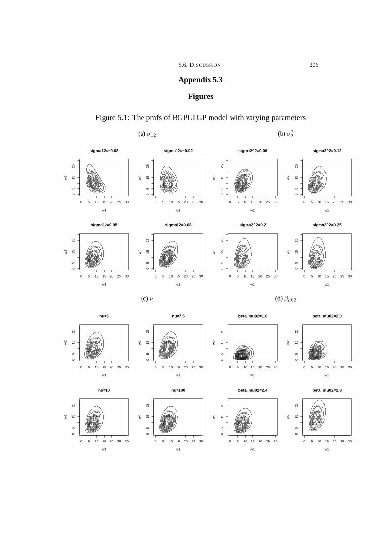
5.6. DISCUSSION 206
Appendix 5.3
Figures
Figure 5.1: The pmfs of BGPLTGP model with varying parameters
(a) σ12
w1
w2
0.001
0.002
0.003
0.004 0.0
05 0
.006
0 5 10 15 20 25 30
05
1525
sigma12=−0.08
w1
w2
0.001
0.002
0.003
0.004
0.0
05
0 5 10 15 20 25 30
05
1525
sigma12=−0.02
w1
w2
0.001
0.002
0.0
03
0.004
0.005
0.007
0 5 10 15 20 25 30
05
1525
sigma12=0.05
w1
w2
0.001
0.002
0.0
03
0.004
0.0
05
0 5 10 15 20 25 30
05
1525
sigma12=0.08
(b) σ2
2
w1w
2
0.001
0.002
0.003
0.0
04
0.0
05
0 5 10 15 20 25 30
05
1525
sigma2^2=0.06
w1
w2
0.001
0.002
0.0
03
0.004
0.0
05
0 5 10 15 20 25 30
05
1525
sigma2^2=0.12
w1
w2
0.001
0.002
0.0
03
0.0
04
0.005
0 5 10 15 20 25 30
05
1525
sigma2^2=0.2
w1w
2
0.001
0.002
0.0
03
0.004
0.0
05
0 5 10 15 20 25 30
05
1525
sigma2^2=0.25
(c) ν
w1
w2
0.001
0.002
0.0
03
0.004
0.0
05
0 5 10 15 20 25 30
05
1525
nu=5
w1
w2
0.001
0.002
0.0
03
0.004
0.0
05
0 5 10 15 20 25 30
05
1525
nu=7.5
w1
w2
0.001
0.002
0.0
03
0.004
0.0
05
0 5 10 15 20 25 30
05
1525
nu=10
w1
w2
0.001
0.002
0.0
03
0.004
0.005
0 5 10 15 20 25 30
05
1525
nu=100
(d) βµ02
w1
w2
0.001
0.0
02
0.0
03 0.004
0.01
0.011
0 5 10 15 20 25 30
05
1525
beta_mu02=1.6
w1
w2 0.001
0.002
0.003
0.0
04 0.009
0 5 10 15 20 25 30
05
1525
beta_mu02=2.0
w1
w2
0.001
0.002
0.0
03
0.004
0.0
05
0 5 10 15 20 25 30
05
1525
beta_mu02=2.4
w1
w2
0.001
0.002
0.0
03
0.004
0.0
05
0 5 10 15 20 25 30
05
1525
beta_mu02=2.8

5.6. DISCUSSION 207
Figure 5.1: The pmfs of BGPLTGP model with varying parameters (con-
tinued)
(e) βa02
w1
w2
0.001
0.002
0.0
03
0.004
0.0
05
0 5 10 15 20 25 30
05
1525
beta_a02=−0.25
w1
w2
0.001
0.002
0.0
03
0.0
04
0.005
0 5 10 15 20 25 30
05
1525
beta_a02=−0.05
w1
w2
0.001
0.002
0.0
03
0.0
04
0.005
0.01
0 5 10 15 20 25 30
05
1525
beta_a02=0.3
w1
w2 0.001
0.002
0.003
0.0
04 0.008
0 5 10 15 20 25 30
05
1525
beta_a02=0.7
(f) λ22
w1
w2
0.001
0.002
0.0
03
0.0
04
0.0
12
0 5 10 15 20 25 300
515
25
lambda22=−0.8
w1
w2
0.001
0.002
0.003
0.0
04
0.0
05
0.0
12
0 5 10 15 20 25 30
05
1525
lambda22=−0.2
w1
w2
0.001
0.002
0.0
03
0.004
0.0
05
0 5 10 15 20 25 30
05
1525
lambda22=0.4
w1
w2
0.001
0.002 0.003
0.004
0.005
0 5 10 15 20 25 300
515
25
lambda22=0.6

5.6. DISCUSSION 208
Figure 5.2: Monthly number of arrests for amphetamine (AMP) and nar-
cotics (NAR) use/possession in Sydney during January 1995 - December
2008
0
10
20
30
40
50
60
Jan-
95
Jul-9
5
Jan-
96
Jul-9
6
Jan-
97
Jul-9
7
Jan-
98
Jul-9
8
Jan-
99
Jul-9
9
Jan-
00
Jul-0
0
Jan-
01
Jul-0
1
Jan-
02
Jul-0
2
Jan-
03
Jul-0
3
Jan-
04
Jul-0
4
Jan-
05
Jul-0
5
Jan-
06
Jul-0
6
Jan-
07
Jul-0
7
Jan-
08
Jul-0
8
month
nu
mb
er o
f ar
rest
s
AMP
NAC

5.6. DISCUSSION 209
Figure 5.3: Trends of the expected monthly number of arrests for use or
possession of two illicit drugs for all fitted models
(a) amphetamine(E(W1t)
)
0
10
20
30
40
50
60
Jan-
95
Jul-9
5
Jan-
96
Jul-9
6
Jan-
97
Jul-9
7
Jan-
98
Jul-9
8
Jan-
99
Jul-9
9
Jan-
00
Jul-0
0
Jan-
01
Jul-0
1
Jan-
02
Jul-0
2
Jan-
03
Jul-0
3
Jan-
04
Jul-0
4
Jan-
05
Jul-0
5
Jan-
06
Jul-0
6
Jan-
07
Jul-0
7
Jan-
08
Jul-0
8
month
nu
mb
er o
f ar
rest
s
AMP
NAC
0
10
20
30
40
50
60
Jan-
95
Jul-9
5
Jan-
96
Jul-9
6
Jan-
97
Jul-9
7
Jan-
98
Jul-9
8
Jan-
99
Jul-9
9
Jan-
00
Jul-0
0
Jan-
01
Jul-0
1
Jan-
02
Jul-0
2
Jan-
03
Jul-0
3
Jan-
04
Jul-0
4
Jan-
05
Jul-0
5
Jan-
06
Jul-0
6
Jan-
07
Jul-0
7
Jan-
08
Jul-0
8
month
nu
mb
er o
f ar
rest
s
observed
BP
BPLN
BPLNGP
BGPLTGP
(b) narcotics(E(W2t)
)
0
10
20
30
40
50
60
Jan-
95
Jul-9
5
Jan-
96
Jul-9
6
Jan-
97
Jul-9
7
Jan-
98
Jul-9
8
Jan-
99
Jul-9
9
Jan-
00
Jul-0
0
Jan-
01
Jul-0
1
Jan-
02
Jul-0
2
Jan-
03
Jul-0
3
Jan-
04
Jul-0
4
Jan-
05
Jul-0
5
Jan-
06
Jul-0
6
Jan-
07
Jul-0
7
Jan-
08
Jul-0
8
month
nu
mb
er o
f ar
rest
s
AMP
NAC
0
10
20
30
40
50
60
Jan-
95
Jul-9
5
Jan-
96
Jul-9
6
Jan-
97
Jul-9
7
Jan-
98
Jul-9
8
Jan-
99
Jul-9
9
Jan-
00
Jul-0
0
Jan-
01
Jul-0
1
Jan-
02
Jul-0
2
Jan-
03
Jul-0
3
Jan-
04
Jul-0
4
Jan-
05
Jul-0
5
Jan-
06
Jul-0
6
Jan-
07
Jul-0
7
Jan-
08
Jul-0
8
month
nu
mb
er o
f ar
rest
s
observed
BP
BPLN
BPLNGP
BGPLTGP

5.6. DISCUSSION 210
Figure 5.4: Trends of the SE of monthly number of arrests for use or pos-
session of two illicit drugs for all fitted models
(a) amphetamine
(√V ar(W1t)
)
0
10
20
30
40
50
60
Jan-
95
Jul-9
5
Jan-
96
Jul-9
6
Jan-
97
Jul-9
7
Jan-
98
Jul-9
8
Jan-
99
Jul-9
9
Jan-
00
Jul-0
0
Jan-
01
Jul-0
1
Jan-
02
Jul-0
2
Jan-
03
Jul-0
3
Jan-
04
Jul-0
4
Jan-
05
Jul-0
5
Jan-
06
Jul-0
6
Jan-
07
Jul-0
7
Jan-
08
Jul-0
8
month
nu
mb
er o
f ar
rest
s
AMP
NAC
0
10
20
30
40
50
60
Jan-
95
Jul-9
5
Jan-
96
Jul-9
6
Jan-
97
Jul-9
7
Jan-
98
Jul-9
8
Jan-
99
Jul-9
9
Jan-
00
Jul-0
0
Jan-
01
Jul-0
1
Jan-
02
Jul-0
2
Jan-
03
Jul-0
3
Jan-
04
Jul-0
4
Jan-
05
Jul-0
5
Jan-
06
Jul-0
6
Jan-
07
Jul-0
7
Jan-
08
Jul-0
8
month
nu
mb
er o
f ar
rest
s
observed
BP
BPLN
BPLNGP
BGPLTGP
0
10
20
30
40
50
60
Jan-
95
Jul-9
5
Jan-
96
Jul-9
6
Jan-
97
Jul-9
7
Jan-
98
Jul-9
8
Jan-
99
Jul-9
9
Jan-
00
Jul-0
0
Jan-
01
Jul-0
1
Jan-
02
Jul-0
2
Jan-
03
Jul-0
3
Jan-
04
Jul-0
4
Jan-
05
Jul-0
5
Jan-
06
Jul-0
6
Jan-
07
Jul-0
7
Jan-
08
Jul-0
8
month
nu
mb
er o
f ar
rest
s
0
2
4
6
8
10
12
14
SE
of
nu
mb
er o
f ar
rest
s
no. of arrests
BP
BPLN
BPLNGP
BGPLTGP
(b) narcotics
(√V ar(W2t)
)
0
10
20
30
40
50
60
Jan-
95
Jul-9
5
Jan-
96
Jul-9
6
Jan-
97
Jul-9
7
Jan-
98
Jul-9
8
Jan-
99
Jul-9
9
Jan-
00
Jul-0
0
Jan-
01
Jul-0
1
Jan-
02
Jul-0
2
Jan-
03
Jul-0
3
Jan-
04
Jul-0
4
Jan-
05
Jul-0
5
Jan-
06
Jul-0
6
Jan-
07
Jul-0
7
Jan-
08
Jul-0
8
month
nu
mb
er o
f ar
rest
s
AMP
NAC
0
10
20
30
40
50
60
Jan-
95
Jul-9
5
Jan-
96
Jul-9
6
Jan-
97
Jul-9
7
Jan-
98
Jul-9
8
Jan-
99
Jul-9
9
Jan-
00
Jul-0
0
Jan-
01
Jul-0
1
Jan-
02
Jul-0
2
Jan-
03
Jul-0
3
Jan-
04
Jul-0
4
Jan-
05
Jul-0
5
Jan-
06
Jul-0
6
Jan-
07
Jul-0
7
Jan-
08
Jul-0
8
month
nu
mb
er o
f ar
rest
s
observed
BP
BPLN
BPLNGP
BGPLTGP
0
10
20
30
40
50
60
Jan-
95
Jul-9
5
Jan-
96
Jul-9
6
Jan-
97
Jul-9
7
Jan-
98
Jul-9
8
Jan-
99
Jul-9
9
Jan-
00
Jul-0
0
Jan-
01
Jul-0
1
Jan-
02
Jul-0
2
Jan-
03
Jul-0
3
Jan-
04
Jul-0
4
Jan-
05
Jul-0
5
Jan-
06
Jul-0
6
Jan-
07
Jul-0
7
Jan-
08
Jul-0
8
month
nu
mb
er o
f ar
rest
s
0
2
4
6
8
10
12
14
SE
of
nu
mb
er o
f ar
rest
s
no. of arrests
BP
BPLN
BPLNGP
BGPLTGP

CHAPTER 6
Summary
6.1. Overview
Longitudinal and panel count data appear in every aspect of our lives
such as in epidemiology, marketing, engineering and economics. The list of
areas in which time series of count data are analyzed is endless. Some com-
mon characteristics of time series of counts include non-stationarity, non-
monotone trends, time-evolving or time-invariant covariate effects, serial
correlation and overdispersion caused by zero-inflation and extreme out-
liers, and population heterogeneity caused by cluster effects in panel data.
Lastly, multiple measurements are sometimes made to each subject at each
time point.
To take into account these properties, Wan (2006) introduced the Pois-
son geometric process (PGP) model to analyze longitudinal and panel count
data. However, the PGP models developed in Wan (2006) looked specifi-
cally into some aforementioned characteristics and did not address other
problems like the serial correlation between observations, overdispersion
and underdispersion. So far, the PGP model has been solely applied to uni-
variate analysis of time series of counts, the multivariate area yet remains
unexplored.
211
6.1. OVERVIEW 212
In light of these, our objective of this research is to extend the PGP
model to allow for those characteristics that have not been addressed. As re-
viewed in Chapter 1, there exist two major categories of models, namely the
observation-driven (OD) and parameter-driven (PD) models which specif-
ically allow for serial correlation. In the OD models, the mean of the out-
come is expressed explicitly as a function of the past observations in order
to construct an autocorrelation structure for accommodating serial correla-
tion. This approach is appealing due to the straightforward prediction and
derivation of the likelihood function. However, difficulties arise when we
interpret the covariate effects on the outcome. On the contrary, the PD
models introduce serial dependence through a latent variable which evolves
independently of the past observations in the mean function and thus en-
ables a straightforward interpretation of the covariate effects. However, the
parameter estimation of this model is computationally intensive due to the
complicated derivation of the likelihood function which involves integra-
tion over the latent variables and the forecasting is cumbersome since the
model is built on a latent process. Unlike the OD and PD models, the PGP
model belongs to the family of the GLMM model and can be classified as
a state space model with state variable Xt where {Xt, t = 1, . . . , n} is the
latent GP evolving independently of the past outcomes. The main differ-
ence between the PGP model and OD/PD models is that the former focuses
on modelling the trend of the time series whereas the latter concentrates on
investigating the serial correlation structure of the outcomes.

6.1. OVERVIEW 213
To combine the merits of these models, we extend the PGP model to
account for serial correlation between observations using the OD model ap-
proach and furthermore to address other characteristics that are prominent
in longitudinal and panel count data. As mentioned before, the mixture
Poisson geometric process (MPGP) model using exponential distribution
as described in Wan (2006) is not adequate to account for excess zeros
and substantial overdispersion. Therefore, firstly in Chapter 2, we propose
two models namely the zero-altered mixture Poisson geometric process
(ZMPGP) model and the mixture Poisson geometric process (MPGP-Ga)
model using gamma distribution to cope with zero-inflation. The ZMPGP
model is essentially a mixture of zero-degenerated model and a zero-truncated
MPGP model via the hurdle approach, while the MPGP-Ga model is a state
space model with state variable E(Wit) = Xit where Xit follows a gamma
distribution. For model comparison, the analysis of bladder cancer data re-
veals that the MPGP-Ga model gives a better model fit than the ZMPGP
model due to the brevity and flexibility of the model distribution. Neverthe-
less, both models are capable of modelling zero-inflated count data but do
so in a different way and therefore are suitable under different situations.
Secondly, concerning another source of overdispersion, the presence
of outlying observations, we pioneer the robust mixture Poisson geometric
process (RMPGP) model in Chapter 3 by replacing the gamma distribution
of the stochastic process {Yit} and assuming the logarithm of the underlying
stochastic process {Y ∗it = lnYit} follows some heavy-tailed distributions
6.1. OVERVIEW 214
including the Student’s t- and exponential power (EP) distributions. The re-
sultant models are namely the RPGP-t and RPGP-EP models. Moreover, by
expressing the two heavy-tailed distributions in scale mixtures (SM) repre-
sentation, the model implementation using MCMC algorithms is facilitated
and the additional parameter known as the mixing parameter enable us to
identify any outliers in the data. For model comparison, the simulation
study shows that the performances of the two RPGP models are comparable
and satisfactory. In case of data with very heavy tail, the RMPGP-t model
seems to fit better since Student’s t-distribution allows a much heavier-than-
normal tail. On the other hand, the RMPGP-EP model allows more diverse
degrees of overdispersion as EP distribution has a more flexible tail which
can be either leptokurtic or platykurtic. Therefore, the latter model gives
a better fit in the analysis of epilepsy data because the two mixture groups
being identified show overdispersion to different extents.
The previous extensions focus on solving the problems related to overdis-
persion, however the analogous problem, underdispersion, has not received
much attention as it is less frequently observed in longitudinal and panel
count data. Nevertheless, a comprehensive count model should contain a
flexible dispersion structure to accommodate different degrees of dispersion
ranging from overdispersion to underdispersion. Therefore, thirdly, we pro-
pose the mixture generalized Poisson geometric process (GMPGP) model
in Chapter 4 which relaxes the restriction of overdispersion in the previ-
ous extended MPGP models. The GMPGP model replaces the Poisson data

6.1. OVERVIEW 215
distribution with generalized Poisson distribution (GPD) which contains an
extra parameter to control the dispersion of the distribution. This unified
model is compared with the RPGP-EP model through two simulation ex-
periments and a real data analysis of the cannabis data. The results high-
light that while the performances of the two models are comparable and
satisfactory in the case of overdispersion, the GMPGP model has a much
better performance in handling underdispersed data in which the RMPGP-
EP model falls short to do so. Moreover in the real data analysis where the
data is overdispersed in the presence of outliers, the GMPGP model still
outperforms the RMPGP-EP model as it can accommodate outliers by the
heavier tail of the generalized Poisson-gamma mixed distribution.
Last but not least in Chapter 5, we explore a new area for the PGP
model on multivariate longitudinal count data by integrating the framework
of RMPGP and GMPGP models. The resultant model named as multi-
variate generalized Poisson log-t geometric process (MGPLTGP) model is
essentially a generalized Poisson mixed model within the GP modelling
framework and adopting multivariate log-t distribution as the mixing den-
sity. Through the real data analysis, we show that the MGPLTGP model
has a couple of merits over some traditional multivariate count models in-
cluding its abilities to handle positive or negative serial, contemporaneous
and cross correlations and accommodate different degrees of dispersion, es-
pecially serious overdispersion due to outlying observations in multivariate
longitudinal count data.

6.2. FURTHER RESEARCH 216
For statistical inference, since the distributions in most of the extended
PGP models do not have a closed-form except the ZMPGP and MPGP-Ga
models, Markov chain Monte Carlo (MCMC) sampling methods are pre-
ferred for parameter estimation to classical approach such as the maximum
likelihood (ML) estimation and the expectation-maximization (EM) algo-
rithm as the former avoids the optimization of high-dimensional likelihood
functions and can be easily implemented using WinBUGS.
In summary, the extended PGP models take into account the serial cor-
relation between observations, overdispersion caused by zero-inflation and
outlying observations, different degrees of dispersion and cross and con-
temporaneous correlations between time series while keeping its old virtue
to accommodate non-stationarity, non-monotone trends, covariate and clus-
ter effects. Accompanied by the straightforward model implementation and
interpretation, these PGP models, which have been applied extensively in
different areas as demonstrated in this research, can undoubtedly compete
with other traditional time series models for count data.
6.2. Further research
In spite of the substantial development of PGP models in this thesis,
there are still many unattended areas that are worthy of further considera-
tion.

6.2. FURTHER RESEARCH 217
6.2.1. Extension to multivariate panel count data. Since many mul-
tivariate longitudinal data comes from panel studies, the presence of popu-
lation heterogeneity is usually inevitable in the data. Hence, the MGPLTGP
model proposed in Chapter 5 which is designed for modelling multivari-
ate longitudinal count data can be further extended to incorporate mixture
effect or random effects to allow for the cluster or subject-specific effects
amongst multiple time series. We believe that the extended mixture model,
which can identify subgroups comprising the population, is useful for all
practical purposes.
6.2.2. Comparison of serial dependence structure. In this research,
we apply the OD model approach in all extended PGP models to accom-
modate the serial dependency between observations by adding some past
observations as covariates into the mean link function of the stochastic pro-
cess {Yit}. On the other hand, we may consider the PD model approach
by incorporating some latent serially correlated random effects which are
independent of past observations into the mean link function. The model
properties of the two diverse approaches can be investigated and compared
in terms of model interpretation, parameter estimation and practicability.
Moreover, when the time series is long, we can consider some simple but
efficient correlation structures to reduce the number of parameters for the
random effects model.

6.2. FURTHER RESEARCH 218
6.2.3. Comparison in methodologies of inference. On the whole, we
focus on the extensions of PGP models to account for different data proper-
ties. Another area that is worthwhile to study is the inference methodology.
Though using MCMC algorithm avoids the evaluation of high-dimensional
likelihood function, the computation time for this sampling algorithms is
sometimes massive if the data size is large and the model is highly compli-
cated.
As an alternative to the ML method in the frequentist approach, the EM
method can be considered since the latent variables are evaluated through
the E-step. Besides, large sample properties of the estimators can be stud-
ied by deriving their large sample distributions. Knowing the asymptotic
distributions, we can then construct confidence intervals for and perform
hypothesis tests on the model parameters.
6.2.4. Comparisons with traditional time series count models. Last
but not least, apart from the model comparison within the extended PGP
models, we can compare our proposed models with those benchmarking OD
and PD models to justify the pros and cons of adopting the PGP approach in
modelling longitudinal and panel count data from different areas. Besides,
knowing the shortcomings, the PGP models can be modified accordingly to
increase its competence among all existing models.

Bibliography
Akaike, H. (1974). A new look at the statistical model identification. IEEE
Transactions on Automatic Control 19, 716-723.
Albrecht, P. (1984). Laplace transforms, Mellin transforms and mixed Pois-
son processes. Scandinavian Actuarial Journal 11, 58-64.
Al-Osh, M.A. & Alzaid, A.A. (1987). First-order integer-valued autoregres-
sive (INAR(1)) process. Journal of Time Series Analysis 8, 261-275.
Angers, J.F. & Biswas, A. (2003). A Bayesian analysis of zero-inflated gen-
eralized Poisson model. Computational Statistics and Data Analysis 42,
37-46.
Aitchinson, J. & Ho, C.H. (1989). The multivariate Poisson-log normal dis-
tribution. Biometrika 75, 621-629.
Australian Institute of Health and Welfare. (2008). 2007 National Drug
Strategy Household Survey: first results. Drug Statistics Series number
20. Cat. no. PHE 98. Canberra: AIHW.
Bae, S., Famoye, F., Wulu, J.T., Bartolucci, A.A. & Singh, K.P. (2005). A
rich family of generalized Poisson regression models with applications.
Mathematics and Computers in Simulation 69, 4-11.
219
BIBLIOGRAPHY 220
Baker, J. & Goh, D. (2004). The cannabis cautioning scheme three years
on: An implementation and outcome evaluation. Drug and Alcohol Co-
ordination, NSW Police, Sydney.
Blumer, M.G. (1974). On the fitting the Poisson-lognormal distribution to
species abundance data. Biometrics 30, 101-110.
Bohning, D., Dietz, E. & Schlattmann, P. (1999). The zero-inflated Poisson
model and the decayed, missing and filled teeth index in dental epidemi-
ology. Journal of the Royal Statistical Society A 162, 195-209.
Box, G.E.P & Tiao, G.C. (1973). Bayesian inference in statistical analysis.
Massachusetts: Addison-Wesley.
Brannas, K. & Johansson, P. (1996). Panel data regression for counts. Sta-
tistical Papers 37, 191-213.
Cameron, A.C. & Trivedi, P.K. (1998). Regression Analysis of Count Data.
Cambridge: Cambridge University Press.
Celeux, G., Forbes, F., Robert, C.P. & Titterington, D.M. (2006). Deviance
information criteria for missing data models. Bayesian Analysis 1, 651-
674.
Chan, J.S.K., Choy, S.T.B. & Makov, U.E. (2008). Robust Bayesian analy-
sis of loss reserve data using the generalized-t distribution. Astin Bulletin
38, 207-230.
Chan, J.S.K., Lam, Y. & Leung, D.Y.P. (2004). Statistical inference for geo-
metric processes with gamma distributions. Computational Statistics and
Data Analysis 47, 565-581.

BIBLIOGRAPHY 221
Chan, J.S.K., Lam, C.P.Y., Yu, P.L.H. & Choy, S.T.B. (2010a), Bayesian
conditional autoregressive geometric process model for range data. Sub-
mitted to a journal for publication.
Chan, J.S.K. & Leung, D.Y.P. (2010). Binary geometric process model for
the modelling of longitudinal binary data with trend. Computational Sta-
tistics, DOI 10.1007/s00180-010-0190-8.
Chan, J.S.K., Wan, W.Y., Lee, C.K., Lin, C.K. & Yu, P.L.H. (2010b). Pre-
dicting dropout and committed first time whole blood donors: the use of
Poisson geometric process model. Submitted to journal.
Chan, J.S.K., Yu, P.L.H., Lam, Y. & Ho, A.P.K. (2006). Modeling SARS
data using threshold geometric process. Statistics in Medicine 25, 1826-
1839.
Chan, K.S. & Ledolter, J. (1995). Monte Carlo EM estimation for time se-
ries models involving counts. Journal of the American Statistical Associ-
ation 90, 242-251.
Chou, R. (2005). Forecasting financial volatilities with extreme values:
The conditional autoregressive range (CARR) model. Journal of Money
Credit and Banking 37, 561-582.
Choy, S.T.B. & Chan, C.M. (2003). Scale mixtures distributions in insur-
ance applications. Astin Bulletin 33, 93-104.
Choy, S.T.B. & Smith, A.M.F. (1997). Hierarchical models with scale mix-
tures of normal distributions. Test 6, 205-221.

BIBLIOGRAPHY 222
Choy, S.T.B. & Walker, S.G. (2003). The extended exponential power dis-
tribution and Bayesian robustness. Statistics and Probability Letters 65,
227-232.
Consul, P.C. (1989). Generalized Poisson distributions: Properties and ap-
plications. New York: Marcel Dekker Inc.
Consul, P.C. & Famoye, F. (1992). Generalized Poisson regression model.
Communications in Statistics - Theory and Methods 21, 81-109.
Consul, P.C. & Jain, G.C. (1973). A Generalization of the Poisson Distribu-
tion. Technometrics 15, 791-799.
Conway, R.W. & Maxwell, W.L. (1962). A queuing model with state de-
pendent service rates. Journal of Industrial Engineering 12, 132-136.
Cox, D.R. (1981). Statistical analysis of time series: Some recent develop-
ments. Scandinavian Journal of Statistics 8, 93-115.
Davis, R.A., Dunsmuir, W.T.M. & Wang, Y. (1999). Modelling time series
of counts. In Asymptotics, nonparametrics, and time series, eds S. Ghosh,
pp. 63-114. New York: Marcel Dekker.
Davis, R.A., Dunsmuir, W.T.M. & Streett, S.B. (2003). Observation-driven
models for Poisson counts. Biometrika 90, 777-790.
Degenhardt, L., Reuter, P., Collins L. & Hall, W. (2005). Evaluating expla-
nations of the Australian ‘heroin shortage’. Addiction 100, 459-469.
Dempster, A.P., Laird, N.M. & Rubin, D.B. (1977). Maximum likelihood
from incomplete data via the EM algorithm (with discussion). Journal of
the Royal Statistical Society B 39, 599-613.

BIBLIOGRAPHY 223
Diggle, P.J. (1988). An approach to the analysis of repeated measurements.
Biometrics 44, 959-971.
Dobbie, M.J. & Welsh, A.H. (2001). Modelling correlated zero-inflated
count data. Australian and New Zealand Journal of Statistics 43, 431-
444.
Efron, B. (1986). Double exponential families and their use in general-
ized linear regression. Journal of the American Statistical Association
81, 709-721.
Faddy, M.J. (1997). Extended Poisson process modelling and analysis of
count data Biometrical Journal 39, 431-440.
Feller, A. (1949). Fluctuation theory of recurrent events. Transactions of the
American Mathematical Society 67, 98-119.
Frei, C. & Schar, C. (2001). Detection probability of trends in rare events:
Theory and application to heavy precipitation in the Alpine region Jour-
nal of Climate 14, 1568-1584.
Freund, D.A., Kniesner, T.J. & LoSasso, A.T. (1999). Dealing with the com-
mon econometric problems of count data with excess zeros, endogenous
treatment effects, and attrition bias. Economics Letters 62, 7-12.
Gilks, W.R., Richardson, S. & Spiegelhalter, D.J. (1996). Markov Chain
Monte Carlo in Practice. UK: Chapman and Hall.
Greenwood, M. & Yule, G. (1920). An inquiry into the nature of frequency
distributions representative of multiple happenings with particular ref-
erence to the occurrence of multiple attacks of Disease or of repeated
BIBLIOGRAPHY 224
accidents. Journal of the Royal Statistical Society A 83, 255-279.
Gupta, R.C. & Ong, S.H. (2005). Analysis of long-tailed count data by
Poisson mixtures. Communications in Statistics - Theory and Methods
34, 557-573.
Hand, D.J., Daly, F., Lunn, A.D., McConway, K.J. & Ostrowski, E. (1994).
A Handbook of Small Data Sets. London: Chapman and Hall.
Hastings, W.K. (1970). Monte Carlo sampling methods using Markov
chains and their applications. Biometrika 57, 97-109.
Heinen, A. (2003). Modeling time series count data: an autoregressive con-
ditional Poisson model. CORE Discussion Paper 2003/62.
Heinen, A. & Rengifo, E. (2007). Multivariate autoregressive modeling of
time series count data using copulas. Journal of Empirical Finance 14,
564-583.
Holla, M. (1966). On a Poisson-inverse Gaussian distribution. Metrika 11,
115-121.
Hur, K., Hedeker, D., Henderson, W., Khuri, S. & Daley, J. (2002). Mod-
eling clustered count data with excess zeros in health care outcomes re-
search. Health Services and Outcomes Research Methodology 3, 5-20.
Jamshidian, M. & Jennrich, R.I. (1997). Acceleration of the EM algorithm
by using quasi-Newton methods. Journal of the Royal Statistical Society
B 59, 569-587.
Johnson, N.L., Kotz, S. & Balakrishnan, N. (1995). Continuous univariate
distributions: Vol. 2. (2nd ed.). New York: Wiley.

BIBLIOGRAPHY 225
Johnson, N., Kotz, S. & Balakrishnan N. (1997). Discrete Multivariate Dis-
tributions. New York: Wiley.
Jones, C., Donnelly, N., Swift, W. & Weatherburn, D. (2005). Driving under
the influence of cannabis: The problem and potential countermeasures.
Crime and Justice Bulletin 87. NSW Bureau of Crime Statistics and Re-
search, Sydney.
Jowaheer, V. & Sutradhar, B.C., 2002. Analysing longitudinal count data
with overdispersion. Biometrika 89, 389-399.
Jowaheer, V., Sutradhar, B.C. & Sneddon, E. (2009). On familial Poisson
mixed models with multi-dimensional random effects. Journal of Statis-
tical Computation and Simulation 79, 1043-1062.
Jung, R.C. & Liesenfeld, R. (2001). Estimating time series models for
count data using efficient importance sampling. Allgemeines Statistisches
Archiv 85, 387-407.
Karlis, D. (2003). An EM algorithm for multivariate Poisson distribution
and related models. Journal of Applied Statistics 30, 63-77.
Karlis, D. & Meligkotsidou, L. (2005). Multivariate Poisson regression with
covariance structure. Statistics and Computing 15, 255-265.
Karlis, D. & Xekalaki, E. (2005). Mixed Poisson distributions. Interna-
tional Statistical Review 73, 35-58.
Karlis, D. & Meligkotsidou, L. (2007). Finite mixtures of multivariate Pois-
son distributions with application. Journal of Statistical Planning and In-
ference 137, 1942-1960.

BIBLIOGRAPHY 226
Kocherlakota, S. (1988). On the compounded bivariate Poisson distribution:
A unified treatment. Annals of the Institute of Statistical Mathematics 40,
61-76.
Kocherlakota, S. & Kocherlakota, K. (1992). Bivariate Discrete Distribu-
tions. New York: Marcel Dekker Inc.
Lam, K.F., Xue, H. & Cheung, Y.B. (2006). Semiparametric analysis of
zero-inflated count data. Biometrics 62, 966-1003.
Lam, Y. (1988a). Geometric process and replacement problem. Acta Math-
ematicae Applicatae Sinica (English Series) 4, 366-377.
Lam, Y. (1988b). A note on the optimal replacement problem. Advances in
Applied Probability 20, 479-482.
Lam, Y. (1992a). Optimal geometric process replacement model. Acta
Mathematicae Applicatae Sinica (English Series) 8, 73-81.
Lam, Y. (1992b). Nonparametric inference for geometric processes. Com-
munications in Statistics: Theory and methods 21, 2083-2105.
Lam, Y. (1995). Calculating the rate of occurrence of failures for
continuous-time Markov chains with application to a two-component par-
allel system. Journal of Operational Research Society 46, 528-536.
Lam, Y. (1997). The rate of occurrence of failures. Journal of Applied Prob-
ability 34, 234-247.
Lam, Y. (2007). The geometric process and its applications. Singapore:
World Scientific Publishing Co. Pte. Ltd.
BIBLIOGRAPHY 227
Lam, Y. & Chan, J.S.K. (1998). Statistical inference for geometric processes
with lognormal distribution. Computational Statistics and Data Analysis
27, 99-112.
Lam, Y. & Zhang, Y.L. (1996a). Analysis of a two-component series system
with a geometric process model. Naval Research Logistics 43, 491-502.
Lam, Y. & Zhang, Y.L. (1996b). Analysis of a parallel system with two
different units. Acta Mathematicae Applicatae Sinica (English Series) 12,
408-417.
Lam, Y. & Zhang, Y.L. (2003). A geometric process maintenance model for
a deteriorating system under a random environment. IEEE Transactions
on Reliability 52, 83-89.
Lam, Y., Zhang, Y.L. & Zheng, Y.H. (2002). A geometric process equiv-
alent model for a multistate degenerative system. European Journal of
Operational Research 142, 21-29.
Lam, Y., Zhu, L.X., Chan, J.S.K. & Liu, Q. (2004). Analysis of data from a
series of events by a geometric process model. Acta Mathematica Appli-
catae Sinica (English Series) 20, 263-282.
Lambert, D. (1992). Zero inflated Poisson regression with an application to
defects in manufacturing. Technometrics 34, 1-14.
Lee, A.H., Wang, K., Scott, J.A., Yau, K.K.W. & McLachlan, G.J.
(2006). Multi-level zero-inflated Poisson regression modelling of corre-
lated count data with excess zeros. Statistical Methods in Medical Re-
search 15, 47-61.

BIBLIOGRAPHY 228
Lee, A.H., Wang, K., Yau, K.K.W., Carrivick, P.J.W. & Stevenson, M.R.
(2005). Modelling bivariate count series with excess zeros. Mathematical
Biosciences 196, 226-237.
Leppik, I.E., Dreifuss, F.E., Bowman-Cloyd, T., Santilli, N., Jacobs, M.,
Crosby, C., Cloyd, J., Stockman, J., Graves, N., Sutula, T., Welty, T.,
Vickery, J., Brundage, R., Gumnit, R. & Guiterres, A. (1985). A double-
blind crossover evaluation of progabide in partial seizures. Neurology 35,
285.
Lunn, D.J., Thomas, A., Best, N., & Spiegelhalter, D. (2000). WinBUGS -
A Bayesian modelling framework: Concepts, structure, and extensibility.
Statistics and Computing 10, 325-337.
Ma, J., Kockelman, K.M. & Damien, P. (2008). A multivariate Poisson-
lognormal regression model for prediction of crash counts by severity,
using Bayesian methods. Accident Analysis and Prevention 40, 964-975.
Mardia, K.V. (1971). Families of bivariate distributions (Griffin’s statistical
monograph No. 27). London: Griffin.
McKenzie, E. (2003). Discrete variate time series. In Handbook of Statistics
21, eds D.N. Shanbhag, C.R. Rao, pp. 573-606. Amsterdam: Elsevier.
McKetin, R., McLaren, J., Riddell, S. & Robins, L. (2006). The relationship
between methamphetamine use and violent behaviour. Crime and Justice
Bulletin No. 97. NSW Bureau of Crime Statistics and Research, Sydney.
Metropolis, N., Rosenbluth, A.W., Rosenbluth, M.N. & Teller, A.H. (1953).
Equations of state calculations by fast computing machines. Journal of

BIBLIOGRAPHY 229
Chemical Physics 21, 1087-1091.
Miaou, S.P. (1994). The relationship between truck accidents and geometric
design of road sections: Poisson versus negative binomial regressions.
Accident Analysis and Prevention 26, 471-482.
Mullahy, J. (1986). Specification and testing of some modified count data
models, Journal of Econometrics 33, 341-365.
Nelder, J. & Wedderburn, R. (1972). Generalized linear models. Journal of
the Royal Statistical Society A 135, 370-384.
Qin, Z., Damien, P. & Walker, S. (1998). Uniform scale mixture models
with applications to Bayesian inference. Working paper #98005, Univer-
sity of Michigan Business School, Michigan.
Quoreshi, A.M.M.S. (2008). A vector integer-valued moving average model
for high frequency financial count data. Economics Letters 101, 258-261.
Ridout, M.S. & Besbeas, P. (2004). An empirical model for underdispersed
count data. Statistical Modelling 4, 77-89.
Smith, A.F.M. & Roberts, G.O. (1993). Bayesian computation via the Gibbs
sampler and related Markov chain Monte Carlo methods. Journal of the
Royal Statistical Society B 55, 3-23.
Snowball, L., Moffatt, S., Weatherburn, D. & Burgess, M. (2008). Did the
heroin shortage increase amphetamine use? A time series analysis. Crime
and Justice Bulletin No. 114. NSW Bureau of Crime Statistics and Re-
search, Sydney.
BIBLIOGRAPHY 230
Spiegelhalter, D.J., Best, N.G., Carlin, B.P. & van der Linde, A. (2002).
Bayesian measures of model complexity and fit (with discussion). Jour-
nal of the Royal Statistical Society B 64, 583-616.
Thall, P.F. & Vail, S.C. (1990). Some covariance models for longitudinal
count data with overdispersion. Biometrics 46, 657-671.
Wakefield, J.C., Smith, A.F.M., Racine-Poon, A. & Gelfand, A.E. (1994).
Bayesian analysis of linear and non-linear population models by using the
Gibbs sampler. Journal of the Royal Statistical Society C 43, 201-221.
Walker, S.G. & Gutiérrez-peña, E. (1999). Robustifying Bayesian proce-
dures. In Bayesian Statistics 6, eds J.M. Bernardo, A.P. Dawid, A.F.M.
Smith, pp. 685-710. New York: Oxford.
Wan, W.Y. (2006). Analysis of Poisson count data using geometric process
model. M. Phil. Thesis, University of Hong Kong, Hong Kong.
Wang, K., Lee, A.H., Yau, K.K.W. & Carrivick, P.J.W. (2003). A bivariate
zero-inflated Poisson regression model to analyze occupational injuries.
Accident Analysis and Prevention 35, 625-629.
Weatherburn, D., Jones, C., Freeman, K. & Makkai, T. (2003). Supply con-
trol and harm reduction: lessons from the Australian heroin ‘drought’.
Addiction 98, 83-91.
Wegman, E.J. (1972). Nonparametric probability density estimation: a
comparison of density estimation methods. Journal of Statistical Com-
putation and Simulation 1, 225-245.

BIBLIOGRAPHY 231
Welsh, A.H., Cunningham, R.B., Donnelly, C.F. & Lindenmayer, D.B.
(1996). Modelling the abundance of rare species: statistical models for
counts with extra zeros. Ecology Modelling 88, 297-308.
Windmeijer, F. (2000). Moment conditions for fixed effects count data mod-
els with endogenous regressors. Economics Letters 68, 21-24.
Winkelmann, R. (2008). Econometric analysis of count Data (fifth edition).
New York: Springer
Xie, F.C., Wei, B.C. & Lin, J.G. (2009). Score tests for zero-inflated gen-
eralized Poisson mixed regression models. Computational Statistics and
Data Analysis 53, 3478-3489.
Yau, K.K.W. & Lee, A.H. (2001). Zero-inflated Poisson regression with
random effects to evaluate an occupational injury prevention programme.
Statistics in Medicine 20, 2907-2920.
Yau, K.K.W., Wang, K. & Lee, A.H. (2003). Zero-inflated negative bino-
mial mixed regression modeling of over-dispersed count data with extra
zeros. Biometrical Journal 45, 437-452.
Zeger, S.L. (1988). A regression model for time series of counts. Biometrika
75, 621-629.
Zeger, S.L., Liang, K.Y. & Albert, P.S.(1988). Models for longitudinal data:
A generalized estimating equation approach. Biometrics 44, 1049-1060.
Zhang, Y.L. (1999). An optimal geometric process model for a cold standby
repairable system. Reliability Engineering and Systems Safety 63, 107-
110.
BIBLIOGRAPHY 232
Zhang, Y.L. (2002). A geometric-process repair-model with good-as-new
preventive repair. IEEE Transactions on Reliability 51, 223-228.
Zhang, Y.L., Yam, R.C.M. & Zuo, M.J. (2001). Optimal replacement pol-
icy for a deteriorating production system with preventive maintenance.
International Journal of Systems Science 32, 1193-1198.
Zhang, Y.L., Yam, R.C.M. & Zuo, M.J. (2002). Optimal replacement policy
for multistate repairable system. Journal of Operational Research Society
53, 336-341.