Embed Size (px)
Citation preview
Extreme value modeling of wind effect on dune erosion on the
Coast of Angelholm
Lionel Arpin-Pont
January 2020

Abstract
The movement of the coast line, due to erosion in one direction or aggregation in theother is a natural process as waves, wind as well as the geological nature of the coast itselfare affecting it. Sand dunes are the main protection coasts have at their disposal againstfloods during storm surges or from more passive but long range rainfalls.
As many of the coastal areas have a dense population and it also shows a great biodi-versity, the dune erosion is a phenomenon worth investigating since it is the destructionof such protection which is vital for everything living close-by. The cost of a flood can bemeasured by human loss, landscape damage or construction loss. Most of the buildings arenot suited for floods.
Studying the dune erosion by itself might not be enough to provide good advice in caseof a surge since the erosion is an effect of the surge as much as it then increases the fol-lowing risks of flooding. In order to be well prepared and build efficient methods againstsuch flooding, it is necessary to better understand the dune erosion and the surroundingphenomenon, such as the sea-level rise, the wave runups or the wind speed.
The data taken for this study comes mostly from the SMHI (Swedish Meteorological andHyrological Institute), taken on or nearby the shore of Angelholm in Skane, south-west ofSweden.
Keywords : Erosion, Wind speed, Extreme value theory, Block maxima, Peaks overthreshold, Copula, Husler-Reiss, Dependence function.
1
Acknowledgement
I would like to thank my supervisor, Nader Tajvidi in Lund University for his time,patience, help and advices throughout my master thesis and for giving me this subjectabout which I had never had been thinking of before, but which has interested me thiswhole semester.
I would also like to thank some of my teachers from Aix-Marseille University in France forthe mathematical knowledge they passed down and the passion they inspired during my ba-chelor ; and my teachers from Lund University for the interest they gave me about statistics.
Finally, I would like to thank my family and friends for their support and help duringmy studies, and more importantly, during this thesis. A special thanks to Thomas Gourdeland Ellen Barrett for proofreading my report.
Last but not least, I want to thank my father who was always by my side and who introdu-ced me to mathematics when I was younger with bed-time stories about strange attractorsand cloud’s trajectories models.
2
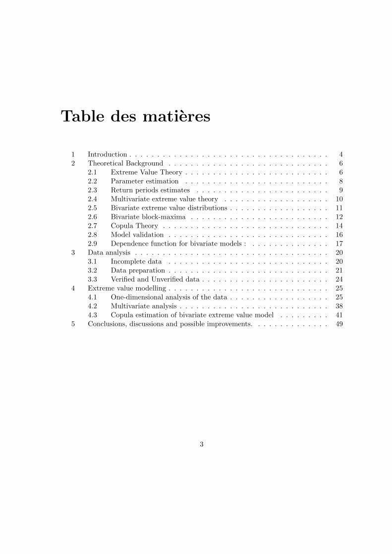
Table des matieres
1 Introduction . . . . . . . . . . . . . . . . . . . . . . . . . . . . . . . . . . . . 42 Theoretical Background . . . . . . . . . . . . . . . . . . . . . . . . . . . . . 6
2.1 Extreme Value Theory . . . . . . . . . . . . . . . . . . . . . . . . . . 62.2 Parameter estimation . . . . . . . . . . . . . . . . . . . . . . . . . . 82.3 Return periods estimates . . . . . . . . . . . . . . . . . . . . . . . . 92.4 Multivariate extreme value theory . . . . . . . . . . . . . . . . . . . 102.5 Bivariate extreme value distributions . . . . . . . . . . . . . . . . . . 112.6 Bivariate block-maxima . . . . . . . . . . . . . . . . . . . . . . . . . 122.7 Copula Theory . . . . . . . . . . . . . . . . . . . . . . . . . . . . . . 142.8 Model validation . . . . . . . . . . . . . . . . . . . . . . . . . . . . . 162.9 Dependence function for bivariate models : . . . . . . . . . . . . . . 17
3 Data analysis . . . . . . . . . . . . . . . . . . . . . . . . . . . . . . . . . . . 203.1 Incomplete data . . . . . . . . . . . . . . . . . . . . . . . . . . . . . 203.2 Data preparation . . . . . . . . . . . . . . . . . . . . . . . . . . . . . 213.3 Verified and Unverified data . . . . . . . . . . . . . . . . . . . . . . . 24
4 Extreme value modelling . . . . . . . . . . . . . . . . . . . . . . . . . . . . . 254.1 One-dimensional analysis of the data . . . . . . . . . . . . . . . . . . 254.2 Multivariate analysis . . . . . . . . . . . . . . . . . . . . . . . . . . . 384.3 Copula estimation of bivariate extreme value model . . . . . . . . . 41
5 Conclusions, discussions and possible improvements. . . . . . . . . . . . . . 49
3
1 Introduction
In this master thesis report, the effect of wind on dune erosion will be dealt with. Thedata come from different stations around the beach of Angelholm, Sweden.
Figure 1 – Picture of the coast of Angelholm from Sanna Ny, on badkartan.se website.
A previous study was done on the effect of wave runups and sea level on the sand dunesof the same region by C. Hallin (2019), ”Long-term beach and dune evolution, Developmentand application of the CS-model”, see [3]. Using 59 different points along the shore over 40years (between 1976 and 2015, included). The analysis will start there to study the effectof wind on dune erosion, to see if and how it amplifies the process. The analysis will bedone using extreme value theory, first with univariate models to get a good grasp at howthose phenomena behave and then with multivariate ones to see how they work together.The theory will be explained in section 2, entitled ”Theoretical Background”.
The goal of this thesis is to provide a better understanding of the influence and effectof the wind on dune erosion on the coast of Angelholm in Sweden, using extreme valuetheory. It will be done by creating a bivariate extreme value model and find quantile for
4
return levels, i.e, the worst case scenario, that is the maximum erosion on the sand dunesin the future.This will be done by finding the most suited data sets from stations surrounding the areaand using extreme value theory to model the erosion using wind speeds and directions. Inthe end, using the results of the analysis of the different data sets, one will be able to seeif there is a risk of flood and damage on the land surrounding Angelholm’s beach.
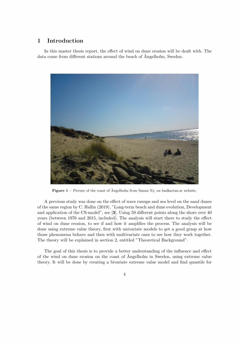
Figure 2 – Diagram of the erosion process with the dune erosion, sea-level rise and the wave run-up.
We start with an introduction to a theoretical part about stochastic processes, bothunivariate and multivariate extreme values models will be introduced as well as some im-portant theory about copulas and goodness of fit methods. Then, dealing with the dataitself : data can, and most of time is, difficult to use as it is. Between missing values oruncertain measurements, choices need to be made. There will be attempts to solve theseproblems. Afterwards, proceeding with the extreme value analysis of the different data sets,from sea-level, maximum wave runups and dune erosion to wind speeds and directions. Atfirst, univariate models will be sought for as one wants to better understand the phenomenaby themselves in order to predict flood risks. And later on, with the wind components, abivariate model will be created for erosion.
During the analysis, the sets used will be the ones which match the best with the re-quirements regarding number of data, period matching, quality and so on, trying to solvethe data-problem in our attempts.
5
2 Theoretical Background
Starting with stationary stochastic processes which are of the most important processesin statistical analysis. A random process is a sequence of random variables X1, X2, ... Theycan either be dependent or not, identically distributed or not. A random process whichhas an homogeneous dependence in time is called a stationary process. Such processes arebroadly studied and are defined below.Definition : A random process X1, X2, ... is stationary if, given integers i1, ...ik and anyinteger m, the joint distribution of {Xi1 , ...Xik} and {Xi1+m, ..., Xi1+m+k} are identical forany choice of m.In other terms, it implies that the mean and the variance of the process are constant overtime and that the covariance function only depends on the shift and not in time, i.e thecorrelation function, defined as
ρ(a, b, t) = corr(X(t+ a), X(t+ b))
and must fulfil the following property
ρ(a, b, t) = ρ(τ), where τ = b− a,∀a, b ∈ N, ∀t ∈ R+ .
2.1 Extreme Value Theory
To begin with, a short introduction to extreme value theory is presented, starting withthe univariate models.
Extreme value theory can be used to model phenomena for which the number of occur-rences is low, as in for example storm surges, floods, financial krach or else, etc. It doesn’trequire to know the distribution function of the occurring phenomena, but only that thedistribution asymptotically converges towards an extreme value distribution. It is used toforecast events to come that are very unlikely but which can happen over a long period oftime, and to prepare for its worst case scenario.
In this paper, extreme value theory will be used for coastal protection. Floods, when oc-curring, can damage coastal cities and landscapes as much as its population. For insuranceand safety reasons, this is a topic of matter now more than in the past as with climatechange, sea-levels rise and floods are even more impacting.
Extreme value analysis is then used to calculate return levels, i.e, levels of a data thatcan be reach in the worst events (as a storm surge or a flood). As there is not much dataon those events, one can use asymptotic arguments to work with extreme values.
In one hand there is the block-maxima method. Let a random process X1, X2, ..., Xn have
6
Mn as its maximum value. Knowing how the {Xi}’s behave would also give Mn’s behavior,but as they are both unknown (for lack of data), one can’t know Mn’s exact distribution.
Hence the following approach
P(X1 ≤ x,X2 ≤ x, ...Xn ≤ x) = Πni=1P (Xi ≤ x) = Fn(x).
F being unknown and G, the limiting distribution of F, is degenerate in xF = supx ∈ R : F (x) < 1,i.e
limn→∞Fn(x) = 0 if x < xF ,
= 1 otherwise.
The issue of degeneration’s leads to the following theorem.
Theorem : Let X1, ..., Xn be a sequence of i.i.d random variables and let Mn be its maxi-mum. If there exist two sequences of constants an > 0 and bn such that
lim P (Mn−bnan
≤ x) = G(x) , as n→∞,
where G is a non-degenerate distribution function, then G belongs to one of the followingthree distribution families :
-Gumbel :
G(x) = e−e−x
, −∞ ≤ x ≤ ∞
-Frechet :G(x) = e(−x)
−α, if x > 0, α > 0
= 1 otherwise;
-Reversed Weibull :G(x) = e−(−x)
−α, if x > 0, α > 0
= 1 otherwise.
To those distributions can be added several parameters like the location parameter µ, thescale parameter σ by changing x to x−µ
σ and the shape parameter ξ = α−1. In the case ofFrechet or Reversed Weibull distributions, α 6= 0, it is 0 for the Gumbel distribution. Toge-ther, they form the GEV distribution family where GEV stands for Generalized ExtremeValue distributions. They share a common form, for which the parameters vary dependingon the most suitable family :
F (x;µ, σ, ξ) = e(−(1+ξ(x−µσ
)− 1ξ ), with µ ∈ R, ξ ∈ R and σ > 0. (1)
7
The type of distribution can be seen by the value of ξ, if ξ = 0 it is a Gumbel (typeI) distribution, ξ > 0, a Frechet (type II) distribution and if ξ < 0, a Reversed Weibull(type III) distribution.
On the other hand, considering only values above a specific threshold, this methodconstrasts with block-maxima which uses maxima in given time intervals. The main ideais to use groups of large values instead of a single one.Let X1, ..., Xn be a sequence of i.i.d random variables having F as distribution functionand let X be a random term from that sequence. Recalling Equation (1), if F meets theasymptotic requirements, then G as in (1) is GEV.
Now fixing a threshold u (suitable threshold being chosen with mean residuals life plots andPOT plots), fitting the conditional distribution of the excedents X − u given that X > ucan be calculated as :
P (X − u > x | X > u) =1− F (u+ x)
1− F (u).
As the distribution of F is unknown, the distribution of the threshold excedences is unknowntoo, see equation (1) and, using Taylor first order approximation of log(F (z)) ' −(1−F (z)),if F (x) ' 1, then we have
1− F (u+ x)
1− F (u)' (1 +
ξ(xσ )
1 + ξ (u−µ)σ
)− 1ξ
= (1 + ξx
σ)− 1ξ , where σ = σ + ξ(u− µ).
For the proof and details, see [1]. As said previously, equations (2.1) are only valid whenF (u) ' 1 or if u is large enough with respect to the support of F . This is called the GPD,for Generalized Pareto Distribution.
2.2 Parameter estimation
The goal of the analysis is to find estimates for the parameters of those extreme valuedistributions GEV and GPD. Under the assumptions of independence and distribution,have
8
-GEV : First, also assuming ξ 6= 0, the log-likelihood function,
log(L(µ, σ, ξ)) = −nlog(σ)− (1 +1
ξ)
n∑i=1
log(1 + ξ(xi − µσ
))−n∑i=1
(1 + ξ(xi − µσ
))− 1ξ
for 1 + ξ(xi−µσ ) > 0∀i ∈ [1, n]
For ξ = 0, as in for Gumbel distributions, the log-likelihood function,
log(L(µ, σ)) = −nlog(σ)−n∑i=1
(xi − µσ
)−n∑i=1
exp(−(xi − µσ
))
-GPD :Gξ,σ(x) = 1− (1 + ξ(
x
σ)− 1ξ ), when ξ 6= 0;
= 1− e−xσ , when ξ = 0.
Recalling σ from (2.1), then let : σ > 0 and x ≥ 0 when ξ ≥ 0 and 0 ≤ x ≤ − σξ when
ξ < 0, giving the log-likelihood function for GPD,
log(L(ξ, σ)) = −nlog(σ)− (1 +1
ξ
n∑i=1
log(1 + (ξxiσ
)), for ξ 6= 0.
When ξ = 0, the exponential case gives
log(L)) = −nlog(σ)−∑i=1n
1 +xiσ
.
Solutions to these maximization problem are not analytical. Numerical solving is most ofthe time used.
2.3 Return periods estimates
Once the parameters have been estimated, one wants to calculate the return level esti-mates, i.e over a period 1
p , such event has a probability of occurring of 1 − p. The longerthe return period, the more likely to happen the event is.
-GEV : By inverting the extreme quantile of the GEV distribution 1 :
xp = µ− σ
ξ(1− (−log(1− p))−ξ), for ξ 6= 0,
= µ− σlog(−log(1− p)), for ξ = 0.
9
-GPD : Similarly,
P (X > x | X > u) = (1 +ξ(xσ )
1 + ξ (u−µ)σ
)− 1ξ;
It follows that
P (X > x) = ζu(1 + ξ(x− uσ
))− 1ξ , with ζu = P (X > u).
The return level xp is the level that is exceeded on average once every p observationsand is solution to
ζu(1 + ξ(xp−uσ ))
− 1ξ =
1
p.
2.4 Multivariate extreme value theory
Proceeding now with the multivariate extreme value theory.Let Xn, n ≥ 1 be an i.i.d
random vector in R, and Xk = (X(1)1 , ..., X
(d)k ), k ∈ [1, n]. The component-wise maxima is
defined as :
Mn = (M (1)n , ...,M (d)
n ) = (maxk∈[1,n]X(1)k , ...,maxk∈[1,n]X
(d)k ). (2)
The interest here, resides in the asymptotic distribution of variable (2). Suppose then that
Xi = (X(1)1 , ..., X
(d)i ) have F (X1, ..., Xn) as distribution function and let
P(Mn ≤ x) = P (X1 ≤ x, ...,Xn ≤ x)
= Fn(x), x ∈ Rd.
The distribution of variable Mn,in equation (2), has a degenerate distribution as Mn → xF ,where xF = sup{x | F (x) < 1}. Under the assumption of existence of the normalizing se-
quences of constants a(i)n > 0 and b
(i)n > 0 for every i ∈ [1, d] and n ≥ 1 such that
P (M
(i)n − b(i)na(i)n
)≤ x(i), i ∈ [1, d]) = Fn(a(1)n x(1) + b(1)n , ..., a(d)n x(d) + b(d)n → G(X(1), ..., X(d)).
The limiting distribution G has each marginal distribution Gi for i ∈ [1, d] being non-degenerate. The ith marginal distribution is
Fni ((a(i)n x(i) + b
(i)n )→ Gi(X
(i)).
10
From univariate results equation (1), each Gi is a member of the GEV family.
2.5 Bivariate extreme value distributions
The most frequently used multivariate extreme value distributions are the bivariateones. Starting with a definition :
Definition : G(x) is max-stable if for every i ∈ [1, d] and every t > 0, there exist func-tions α(i)(t) and β(i)(t) strictly positives such that
Gt(x) = G(α(1)(t)x(1) + β(1)(t), ..., α(d)(t)x(d) + β(d)(t)).
It can be shown that G(x) is max-stable if and only if it is a multivariate extreme valuedistribution. Thus one needs to find all possible multivariate max-sable distribution, assu-ming one of the three possible univariate marginal extreme valued distribution. Also canbe shown that any bivariate extreme value distribution with unit Frechet margins can bewritten as
G∗(x, y) = e(−( 1
x+ 1y)A( x
x+y))
, (3)
where A(ω) is called the dependence function. Since (3) has unit Frechet margins, we have
limx→∞G∗(x, y) = e− 1y and
limy→∞G∗(x, y) = e−1x ;
withGn∗ (x, y) = G∗(
x
n,y
n).
Implying that G∗(x, y) is max-stable. It can also be shown that Gt∗(xt, yt) = G∗(x, y), fort > 0.
It can be shown that the dependence function A(ω) has the following properties :
1. A(0) = A(1) = 1 ;
2. max(ω, 1− ω) ≤ A(ω) ≤ 1, if 0 ≤ ω ≤ 1 ;
3. A(ω) is convex for ω ∈ [0, 1].
A has lower boundA(ω) = 1− ω, for ω < 1
2 ,
= ω, otherwise,
11
and upper bound A(ω) = 1.There is no parametric family which gives all possible bivariate extreme value distribution.
Starting there with the R-package evd, there are 9 different parametric bivariate extremevalue models. Listed in the following subsection. One first needs a finite form for the mar-ginal distributions :
yi = yo(xi) = {1 + ξi(xi − yiσi
)}−1ξi , for i = 1, 2
where the marginal parameters are (µi, σi, ξi), with ξi > 0.If ξi = 0, yi is defined by continuity.
In each of the 9 parametric bivariate distribution functions G given below, the univa-riate margins belong to the GEV family as explained earlier.Choosing an appropriate block-size for the block-maxima as it is the kind of model we wantto fit to our data.
2.6 Bivariate block-maxima
We will proceed the analysis using a bivariate model for erosion and oriented windspeed. Due to the format of the data available, we will use component-wise block maximamodels, with as before, blocks of one year (starting January, the 1st until December, the31st).
Suppose there is (X1, Y1), (X2, Y2), ... a sequence of vectors that are independent ver-sions of a random vector (X,Y ) having distribution F (x, y), then define as previouslythe component-wise maxima :
Mn = (maxi=1:n(Xi),maxi=1:n(Yi))
= (Mx,n,My,n)
Note that it is a component-wise maxima vector, i.e, this vector does not have to be anobserved vector from the original series of data. The two maxima may have been observedat different moments in the block.
— log : The bivariate logistic distribution function is defined as :
G(x,y) = exp{−{x1r + y
1r }r},
12
where r ∈ [0, 1]. Independence when r = 1, dependence when r tends to 0. This isa special case of the alog model (following model).
— alog : The bivariate asymetric logistic distribution function is defined as :
G(x,y) = exp{−(1− t1)x− (1− t2)y − {(t1x)1r + (t2y)
1r }r},
where r ∈ [0, 1], t1 ≥ 0 and 1 ≥ t2. Independence is either when r = 1 and t1 = 0 ort2 = 0. Dependence when r tends to 0 and t1 = t2 = 1.This is the origin of the special case of the log model (previous model), as in wheret1 = t2 = 1. Different limits occur when t1 and t2 are fixed and r tends to 0.
— hr : The Hustler-Reiss distribution function is defined as :
G(x,y) = exp{−xφ(1
r+ r(log
x
y))− yφ(
1
r+ r(log
y
x))}
where φ is the standard normal distribution function and r > 0. Independence isobtained when r tends to 0. Dependence when r tends to ∞.
— neglog : The bivariate negative logistic distribution function is defined as :
G(x,y) = exp{−x− y + (x−r + y−r)−1r }
where r > 0. Independence is when r tends to 0 and dependence when r tends to∞. This is a special case of the aneglog model (following model).
— aneglog : The bivariate asymmetric negative logistic distribution function is definedas :
G(x,y) = exp{−x− y + ((t1x)−r + (t2y)−r)−1r }
where r > 0, t1 ≥ 0 and 1 ≥ t2. Independence is when either r,t1 or t2 tends to 0and dependence when t1 = t2 = 1 and r tends to ∞.This is the origin of the special case of the neglog model (previous model), as inwhere t1 = t2 = 1. Different limits occur when t1 and t2 are fixed and r tends to 0.
— bilog : The bivariate bilogistic distribution function is defined as :
G(x,y) = exp{−{xq1−α + y(1− q)1−β}r},
where q is the root of the following equation :
(1-α)x(1− q)β − (1− β)yqα = 0
13
where 0 < α and β < 1. Independence when α = β approaches 1. Dependence whenα = β tends to 0. Different limits occur when α or β is fixed and the other tendsto 0. This is a special case of the log model (g.1) when α = β and then to the alogmodel (g.2) with also t1 = t2 = 1.
— negbilog : The bivariate negative bilogistic distribution function is defined as :
G(x,y) = exp{−x− y + xq1+α + y(1− q)1+β}r},
where q is the root of the following equation :
(1+α)xqα − (1 + β)y(1− q)β = 0
where α,β > 0. Independence when α = β approaches ∞. Dependence when α = βtends to 0. Different limits occur when α or β is fixed and the other tends to 0. Thisis a special case of the neglog model (g.1) when α = β and with reformulation 1
αand 1
β .— ct : The Coles-Tawn distribution function is defined as :
G(x,y) = exp{−x(1−Be(q;α+ 1, β))− yBe(q;α, β + 1)}, where
α,β < 0 and q =yα
yα+ xβ.
Be(q;α, β) is the Beta distribution function evaluated at q. Independence is whenα = β approaches 0 or when one of α, β is fixed and the other tends to 0. Dependenceis when α = β tends to ∞. Different limits occur when one of α, β is fixed and theother tend to ∞.
— amix : The asymmetric mixed distribution function is defined as :
A(t) = 1− (α+ β)t+ αt2 + βt3
where α ≥ 0 and +3β ≥ 0, or where α + β ≤ 1 and α + 2β ≤ 1. Then,α ∈ [0, 1.5]and β ∈ [−0.5, 0.5].Although α→ 1 implies β < 0.Independence is when α = β = 0. Dependence is when α increases and β is fixed,although complete dependence can’t be reached.
2.7 Copula Theory
A bivariate model is needed for the wind speed and the erosion, and for such, the copulatheory provides an alternative way of creating models, i.e. : Extreme value copula models.Below, a summary of the copula theory is provided but refer to [2] for more informationon this topic.
14
The main idea of copulas can be explained as the following : When the joint distributionfunction is hard to find or to use, copulas are a way of having the joint distribution as afunction of the marginal distributions. Later on in this report using a copula and the twomarginal distributions a model for oriented windspeed and erosion will be created.Let (X,Y ) coming from a F (x, y) distribution, with F : R2 → [0, 1]. And define C :[0, 1]2 → [0, 1].
F (x, y) = C(F1(x), F2(y)),
with F1 and F2 the respective marginal distributions of the random variablesX and Y.
Then, a d-dimensional copula is defined for d ≥ 2 such that it is a function C : [0, 1]2 → [0, 1]for which
∃(U1, ..., Ud) such that, Ui ∼ U(0, 1)∀i ∈ [1, d],
and
C(u1, ..., ud) = P (U1 ≤ u1, ..., Ud ≤ ud).
Also, the copula associated with F is defined for F : Rd → [0, 1],
C(u1, ..., ud) = F (F1(u1)−1, ..., Fd(ud)
−1),
where F1, ..., Fd are the marginal distributions of F.
The next step is the most important theorem about copulas, Sklar’s theorem
Theorem : Let F be a joint distribution function with marginals F1, ..., Fd. Then, thereexists a copula C such that
F (X1, ..., Xd) = C(F1(X1), ..., Fd(Xd))
And conversely, if C is a copula and F1, ..., Fd are distribution functions, then it is a jointdistribution function with marginals F1, ..., Fd.
There are three other important consequences concerning the last theorem :
— C explains the dependence between the margins ;— a joint distribution functions can be split in two parts, its margins and its copulas.
Hence, they can be modelled separately ;
15
— for a given copula C, the margins can be freely changed, for example, C(H1(X1), ...,Hd(Xd))is a proper distribution function.
Aside from Sklar’s theorem, it can be shown that any measure of dependence which de-pends only on a copula, does not change under strictly increasing transformations. Whichgives us Kendall’s τ , and Spearmann’s ρ dependence measures.
An extreme-value copulas is then defined as :
Definition : Any copula for which Ct(u, v) = C(ut, vt), ∀t > 0, is called an extreme-valuecopula. This also applies to any dimension d ≥ 2, where Ct(u1, ..., ud) = C(ut1, ..., u
td).
It can be shown using a bivariate GEV with unit Frechet margins G∗ that
C(u, v) = exp(log(uv)A(log(u)
log(uv)),
with A a convex function called dependence function and u, v in [0, 1].
From that definition, can be found the different extreme value copulas like the Gumbel,Galambos, Tawn, t and Husler-Reiss.
2.8 Model validation
As one creates models to fit the data, one also needs to check if the fit is good en-ough. In this analysis, the ”fit diagnostic plot” function from the in2extRemes R packagewill be mostly used for the univariate part. But one can also use various criteria such asp− value,AIC and BIC, or dependence functions for bivariate models.
Definition : The Akaike Information Criteria (AIC) is commonly use for model orderselection. The value of AIC is based on information theory, rewarding a high likelihood ofthe model but penalizing an high model order. The lower the AIC is, the better the modelis (but it is NOT a sign that the model is good, just that it is better than other models witha higher AIC).
AIC = −2log(L) + 2k,
with L the likelihood function and k the number of parameters in the model.
Definition : The Bayesian Information Criteria (BIC), works like the AIC above. A lower
16
BIC indicates a better model (same note as for AIC about how good the model is, BIC isnot a quality indicator but an efficiency one)
BIC = −2log(L) + log(n)k
with L the likelihood function, n the number of observations and k the number of parame-ters in the model.
Those information criterion, AIC and BIC are not a measure of goodness of fit and onedoesn’t penalize over-fitting(AIC) where the other doesn’t penalize under-fitting(BIC).They are indicators of which models is the best but not if a model is good.
Fit Diagnostic : Let x1, ..., xn denote a sample of i.i.d observations with distribution F .Have F , an estimate of F . The empirical function is defined by
F(x) =i
n+ 1, for x ∈ [x(i), x(i+1)].
As F is an estimate of the true probability distribution function F , it should be similarto the estimated model F . Comparing F with F shows various goodness of fit procedures,where probability plot and quantile plot are the two most commonly used graphical tech-niques.
— A probability plot is the set of points ((F (x(i)),i
n+1), i ∈ [1, n]) ;
— A quantile plot is the set of points ((F−1( in+1), x(i)), i ∈ [1, n]) ;
If F is a good enough estimate, the probability plot and the quantile plot will be closeenough from the diagonal unit line. Opposed to the AIC and BIC, those graphical me-thods for goodness of fit show whether a model is good enough, but doesn’t say anythingon it’s efficiency about the number of parameters.
2.9 Dependence function for bivariate models :
Now going to go quickly through several methods of estimating the dependence func-tion, which is a good way of assessing the goodness of fit of a model onto the data. Startingwith Non-Parametric estimation of dependence function.
Suppose (X,Y ) ∼ G∗(x, y), a couple of random variables and (x1, y1), ..., (xn, yn) a sample ;
17
I).Non-parametric methods :
i). Pickand’s estimator(1981) :It can be shown that min( 1
(1−ω)X ,1Y ω ) ∼ exp(A(ω)), where A(ω) is the dependence func-
tion. Defining Zi(ω) = min( 1(1−ω)Xi ,
1Yiω
), one can get :
Ap(ω) =n∑n
i=1 zi(ω)
Although, even if this estimator is good asymptotically, the reality of the data makes thisestimator quite inaccurate. There is a modified version of this estimator defined later on.
ii). Caperaa, Fougeres and Genest’s (CFG) estimate (1997) :Take (Ui, Vi) ∼ (F1(Xi), F2(Yi)),∀i ∈ [1, n].The CFG estimator of the dependence function is :
An(ω) = (1− ω)Q1−p(ω)n , if ω ∈ [0, Z(i)]
= ωi/n(1− ω)1−i/nQ1−p(ω)n Q−1i , if ω ∈ [Z(i), Z(n)]
= ωQ−p(ω)n , if ω ∈ [Z(n), 1].
Where Qi = {Πik=1
Z(k)
(1− Z(k)}
1n , ∀i ∈ [1, n].
II). Maximum likelihood based on parametric models :
iii). Hall-Tajvidi modification of the Pickand’s estimator :By changing Xi = 1
Xiand Yi = 1
Yi, have
Bp−HT (ω) =
∑ni=1min( xi
(1−ω)E[X], yi(1−ω)E[Y ]
)
n
iv). Constrained smoothing splines :
A can be approximated by a spline that is constrained to satisfy all the necessary conditionsof the dependence function, bu choosing regularly spaced points from t0 = 0, to tm = 1,all points being strictly smaller than the next one, spanning the interval [0, 1].
Then, with s > 0, one has to find As, the polynomial of degree 3 or more that mini-mizes :
18

m∑j=1
(A(tj)− As(tj))2 +
∫ 1
0A′′s(t)
2dt (4)
As mentioned previously, this function satisfies the dependence function requirements.
For more details about the theory behind stationary stochastic processes, see [8] ; for ex-treme value theory, see [1] ; finally, and for copula theory, see [2].
19
3 Data analysis
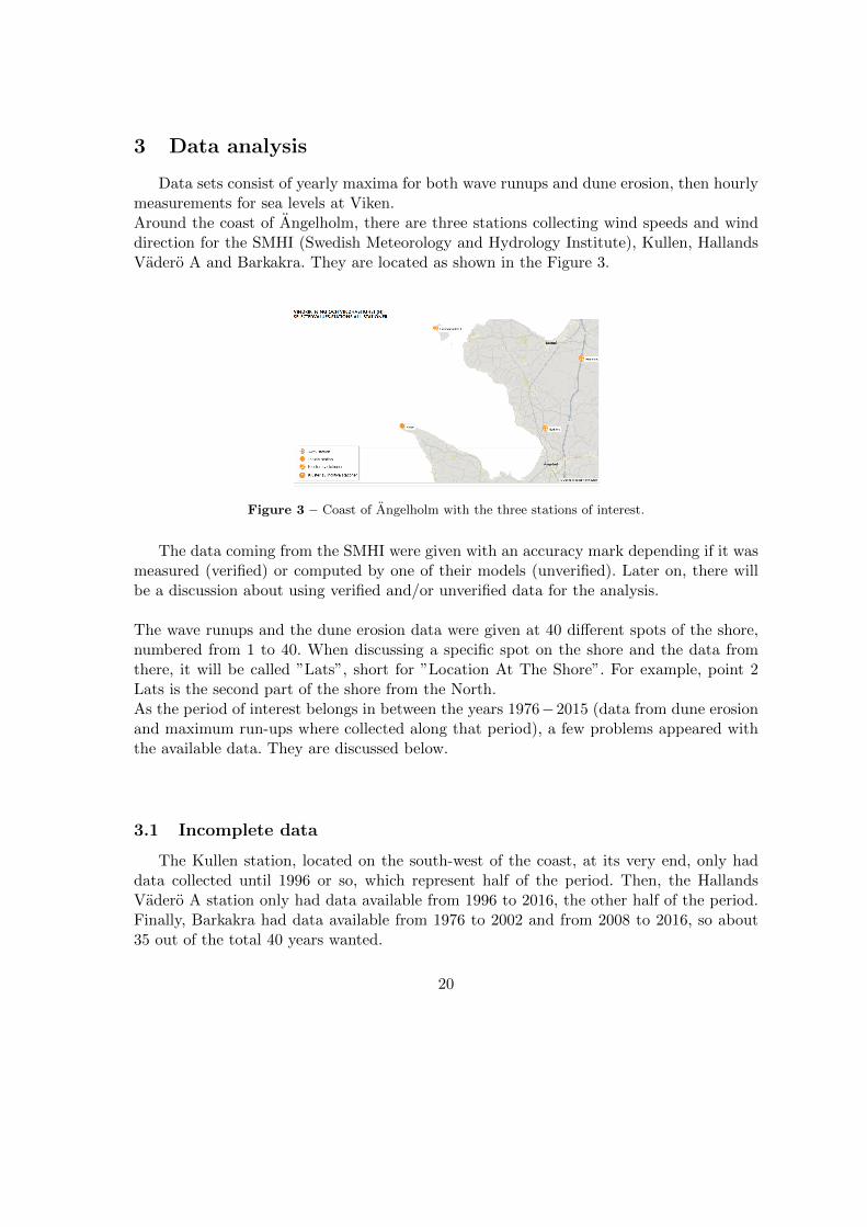
Data sets consist of yearly maxima for both wave runups and dune erosion, then hourlymeasurements for sea levels at Viken.Around the coast of Angelholm, there are three stations collecting wind speeds and winddirection for the SMHI (Swedish Meteorology and Hydrology Institute), Kullen, HallandsVadero A and Barkakra. They are located as shown in the Figure 3.
Figure 3 – Coast of Angelholm with the three stations of interest.
The data coming from the SMHI were given with an accuracy mark depending if it wasmeasured (verified) or computed by one of their models (unverified). Later on, there willbe a discussion about using verified and/or unverified data for the analysis.
The wave runups and the dune erosion data were given at 40 different spots of the shore,numbered from 1 to 40. When discussing a specific spot on the shore and the data fromthere, it will be called ”Lats”, short for ”Location At The Shore”. For example, point 2Lats is the second part of the shore from the North.As the period of interest belongs in between the years 1976−2015 (data from dune erosionand maximum run-ups where collected along that period), a few problems appeared withthe available data. They are discussed below.
3.1 Incomplete data
The Kullen station, located on the south-west of the coast, at its very end, only haddata collected until 1996 or so, which represent half of the period. Then, the HallandsVadero A station only had data available from 1996 to 2016, the other half of the period.Finally, Barkakra had data available from 1976 to 2002 and from 2008 to 2016, so about35 out of the total 40 years wanted.
20
Also, the yearly maximum erosion has many of 0-values which makes the analysis moredifficult.
3.2 Data preparation
As parts (often very consequent ones) of the data are missing, it is required to find away to get around. The following list consists of the various ideas of data preparation thatwas, or could have been, used in this analysis ; they come with different advantages as wellas disadvantages. Some of them use, for example (b.1) and (b.2) use the data as available,i.e reduced data sets, where the other alternatives are ways to get a more complete set butthat may require strong assumptions that can be hard to fill in correctly.They are as follow :
— b.1 : Only using 20 years of data instead of 40, then, one can either use the datafrom Kullen or Barkakra for the first 20 years, or from Hallands Vadero A for thelast 20 years, depending on which period is the most interesting.
Problem (b.1) :The period is somewhat short and if a block maxima model appears to be the best,the accuracy will decline due to low amounts of data. Also, as the previous studywas made on the whole 40 years, it would be better to aim for consistency ;
— b.2 : Barkakra’s set has the most years available, but as they are not consecutive,they may not be usable as they are. Although, checking whether the set is stationaryenough would make it usable.
Problem (b.2) :It would still be 35 years instead of 40 years, lowering the accuracy of the results ;
— b.3 : Have a mix of them, i.e use 20 years of one and 20 years of the other, which,grouped, would make a whole 40 years data set as they conveniently cover eachother’s gap. There is even have a choice between Barkakra and Kullen for the firstpart, choosing the one that shows the most correlation with Hallands Vadero A toget a significantly close set. As the stations are part of the same coast, their pro-perties could be similar.
Problem (b.3) :They are not. Sets that are significantly close are needed. Especially that, lookingat the data, one can see that the wind speeds are very different (much higher) atHallands Vadero A than at the others. Mixing the data sets as proposed might not
21
be relevant ;
A mix of the 3 sets seems rather inefficient, as it would be : 20 years from Kul-len (1976 − 1996), 6 years from Barkakra (1997 − 2002), 5 years from Hallands(2003 − 2008) and the final years from Barkakra again (2009 − 2015). This case ispositively useless as it takes the flaws of pretty much all other combinatory alterna-tives and doesn’t gain any of its advantages other than having a full 40-years set.
— b.4 : A different mixing could be done by using the set from Barkakra and using 5years from another station (Hallands Vadero A for example) to cover its gap. AsBarkakra is the set with the most usable years by far, it would make more sensethan the previous two alternatives (b.2) and (b.3). It also is the closest station fromthe actively eroded zones Lats.
Problem (b.4) :Same as (b.3).
— b.5 : Then, rather than directly using data from Hallands Vadero A to covers Bar-kakra’s gap, one could simply reconstruct Barkakra’s missing 6 years by creatinga model that fits Barkakra’s data. Either by using Hallands Vadero A station tohelp (like in a Box-Jenkins model, see [7]) or without, by using a Kalman filter tomake the reconstruction, knowing that wind speeds can be modelled via a Weibulldistribution.
Problem (b.5) :Such a reconstruction might be too much of a hassle and give questionable results,where alternative (b.4) is simpler but also seems efficient enough. Using such me-thods to re-create a maximum of 5 points (approximately from the years 2002−2008)appears tedious, at best.
Other than the faulty wind data, the yearly maxima for erosion show values andbehaviours that are not easy to use. Most of the data points are 0-valued, makingthe analysis intricate. By grouping them or using blocks of several years (no morethan two preferably), the erosion data becomes more usable even though the num-ber of data depletes fast.
— b.6 : Instead of using 40 years of data, i.e 40 yearly maxima, one could use half (20)and take a block size of two-years instead of one.
Problem (b.6) :
22
Having 20 points instead of 40 may be too small an amount for the analysis to workproperly.
— b.7 : As a way of minimizing the faulty erosion data, instead of choosing one spotLats, one could pick three neighbouring spots Lats and take the yearly maximumover those 3 ones. As they are close to each other, the values should be concordantand somewhat take care of most of the 0s. The ad hoc spots would then be spots 9to 11 Lats, but still represent 10 different 0-valued points.
Problem (b.7) :Are they close enough ? If they are, the erosion being 0 somewhere might imply theerosion would be 0 on the other points too. It also represent a quarter of the wholedataset being 0, which is too much.
— b.8 : Taking the maximum erosion over the whole bay (all spots Lats) so the chancesof having 0s should be significantly reduced.
Problem (b.8) :It actually is not. The 0-values on yearly erosion seem to be unrelated to the spotLats but related to specific years. Using a maximum along every spot Lats doesn’tsolve that problem.
Following from last approach, (b.8), a block size of two years will be taken for ero-sion over the whole bay . Calculations in the next part show that the maxima areactually located around spots Lats 9 to 11, hence that a maxima over the whole bayis the same as a maxima over those three spots Lats.
As a final note on those alternatives, trying to get data on a shifted period, as in 1979−2019for all the data sets (wind speeds, wind directions, erosion, wave run-ups and sea levels)would not be of any help at solving the above problems.
This paper will only contain the most successful attempt and a comparison between themodels created with this approach. That means the data processing that will take intoaccount the smallest confidence intervals, the significance of the parameters and the fit tothe data for example.For this analysis, the alternatives (b.4), (b.6) and (b.8) will be used, i.e, filling Barkakra’sdata set gap with Hallands Vder data and using the maximum erosion over the whole bay.The amount of manipulations done on the data was deemed necessary to get functioningmodels, the other attempts were only ending in insignificant models.
23
3.3 Verified and Unverified data
To add to the previous section on missing data, there is a certainty, or accuracy problem.
The wind data as they were collected and stored were given the status ”Verified (G)”or ”Unverified(Y)”, as ”G” means ”kontrollerade och godknda vrden” (or ”checked andapproved values”) where ”Y” means ”misstnkta eller aggregerade vrden. Grovt kontrolle-rade arkivdata och okontrollerade realtidsdata (senaste 2 tim)” (or ”suspicious or aggre-gated values. Roughly controlled archive data and uncontrolled real-time data (in the last2 hours)”).
Also with it came some data that had G-valued wind speeds but Y-valued wind direc-tions (or vice-versa). One can, either consider such an event as a Y-valued data vector ifone uses both wind speed and wind direction, or as G-valued if one only uses the G-valuedcomponent data in the vector. Although, both components will be used during the analysis,and therefore, the whole vector is to be referred as Y-valued.
By checking the yearly maxima of those data sets, it revealed that a significant amount ofthem were stated in the Y category, hence were unverified. 50% of Hallands Vadero’s setfor yearly maxima contains unverified values. The same ratio is true for the other sets. Asit is half of them being unverified, one can wonder if running an analysis with that manyuncontrolled values is worth anything.
It is now a question of whether to use all the data or only the verified ones. Although,for the latter, another problem would rise as the frequency of apparition of those unverifieddata may not be from a special or predictable pattern, hence there would be years withless values than others. Depending on the analysis, that can be problematic.
As a consequence of not wanting to have different amounts of data in each year, and,more importantly, even if the data is unverified, it can be the true value or significantlyclose to the true value. As the quality of the models made by SMHI cant be judged, thedata was kept, regardless of verified status.
24
4 Extreme value modelling
As two of our data sets (dune erosion and wave run-up) are yearly maxima, they arebest fitted for the block maxima models. Trends and seasonal cycles can’t be seen fromany plot in the data because of its nature. Both data sets consists of 59 points spreadhomogeneously along the shore with 40 yearly maxima (years 1976− 2015).
The block size is chosen from the available data, that is that the blocks should be cutin years, from the 1st of January to the 31st of December of that year. Although, for thebivariate model between dune erosion and oriented wind speed, a lack of non-0 values willshow up and create problems with the model ; hence a change needs to be made and amaximum over two-years sized blocks instead of one-year sized blocks is used in order tominimize their impact on the model.
A significance level of 5% was chosen to concur with results from other studies and makeit easier to compare as it is the most commonly used. All univariate block-maxima mo-dels have been tested for GEV distribution against Gumbel distribution. For peaks overthreshold, models with shape = 0 are tested against exponential distributions. Whateverdistribution fitting the most the data will be kept according to likelihood-ratio-tests, andthe other rejected. Unless specified otherwise, all confidence intervals will be calculatedusing normal approximation from the R-package in2extremes.
4.1 One-dimensional analysis of the data
The first two parts of this section will be dealing with sea-level rise and wave runups.The two of them together, by simple addition of the return levels will give the potentialrisk of flooding, i.e, if the wave height leveled up by the sea level, bypass the sand dunesheight, there is a risk of flood.
The last part of this section will be dealing with the erosion, and wind components, speedand direction. A univariate analysis will be performed to first understand how wind anderosion behave on their own and then in the later multivariate analysis section to confirmthe effect of wind on dune erosion.
On to sea level
The sand dune is the main protection against flooding. As long as the sea-level or thewave height is lower than the dune height, coastal cities and lands will not be damaged. Foran in depth analysis of the dune themselves, see [3], Long-term beach and dune evolution,2019.
25
Here, only use extreme value analysis will be used in regards to the sea-level and thenon to wave runups, rather than an analysis on the global shape and parts of the dune andhow both sea level and wave height impact them.
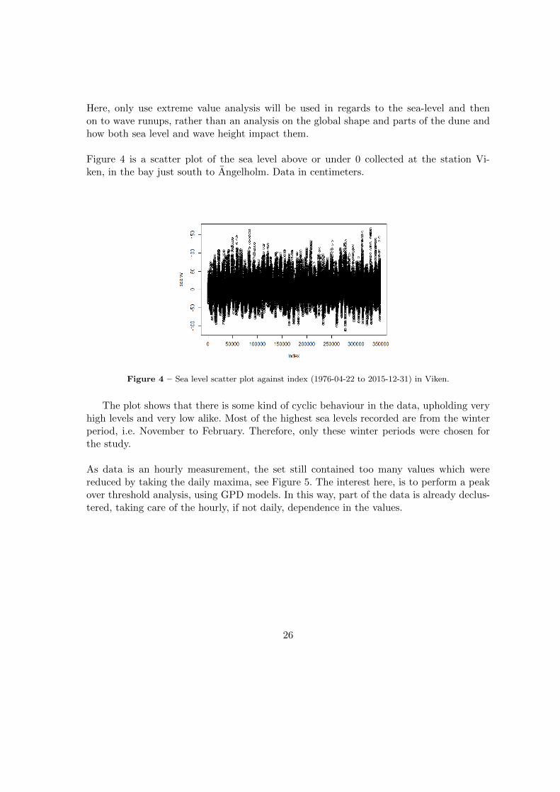
Figure 4 is a scatter plot of the sea level above or under 0 collected at the station Vi-ken, in the bay just south to Angelholm. Data in centimeters.
Figure 4 – Sea level scatter plot against index (1976-04-22 to 2015-12-31) in Viken.
The plot shows that there is some kind of cyclic behaviour in the data, upholding veryhigh levels and very low alike. Most of the highest sea levels recorded are from the winterperiod, i.e. November to February. Therefore, only these winter periods were chosen forthe study.
As data is an hourly measurement, the set still contained too many values which werereduced by taking the daily maxima, see Figure 5. The interest here, is to perform a peakover threshold analysis, using GPD models. In this way, part of the data is already declus-tered, taking care of the hourly, if not daily, dependence in the values.
26
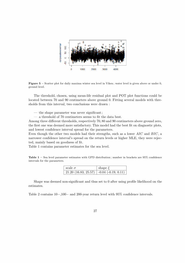
Figure 5 – Scatter plot for daily maxima winter sea level in Viken ; water level is given above or under 0,ground level.
The threshold, chosen, using mean-life residual plot and POT plot functions could belocated between 70 and 90 centimeters above ground 0. Fitting several models with thre-sholds from this interval, two conclusions were drawn :
— the shape parameter was never significant ;— a threshold of 70 centimeters seems to fit the data best.
Among three different thresholds, respectively 70, 80 and 90 centimeters above ground zero,the first one was deemed more satisfactory. This model had the best fit on diagnostic plots,and lowest confidence interval spread for the parameters.Even though the other two models had their strengths, such as a lower AIC and BIC, anarrower confidence interval’s spread on the return levels or higher MLE, they were rejec-ted, mainly based on goodness of fit.Table 1 contains parameter estimates for the sea level.
Table 1 – Sea level parameter estimates with GPD distribution ; number in brackets are 95% confidenceintervals for the parameters.
scale σ shape ξ
21.20 (16.83, 25.57) -0.04 (-0.19, 0.11)
Shape was deemed non-significant and thus set to 0 after using profile likelihood on theestimates.
Table 2 contains 10−,100− and 200-year return level with 95% confidence intervals.
27
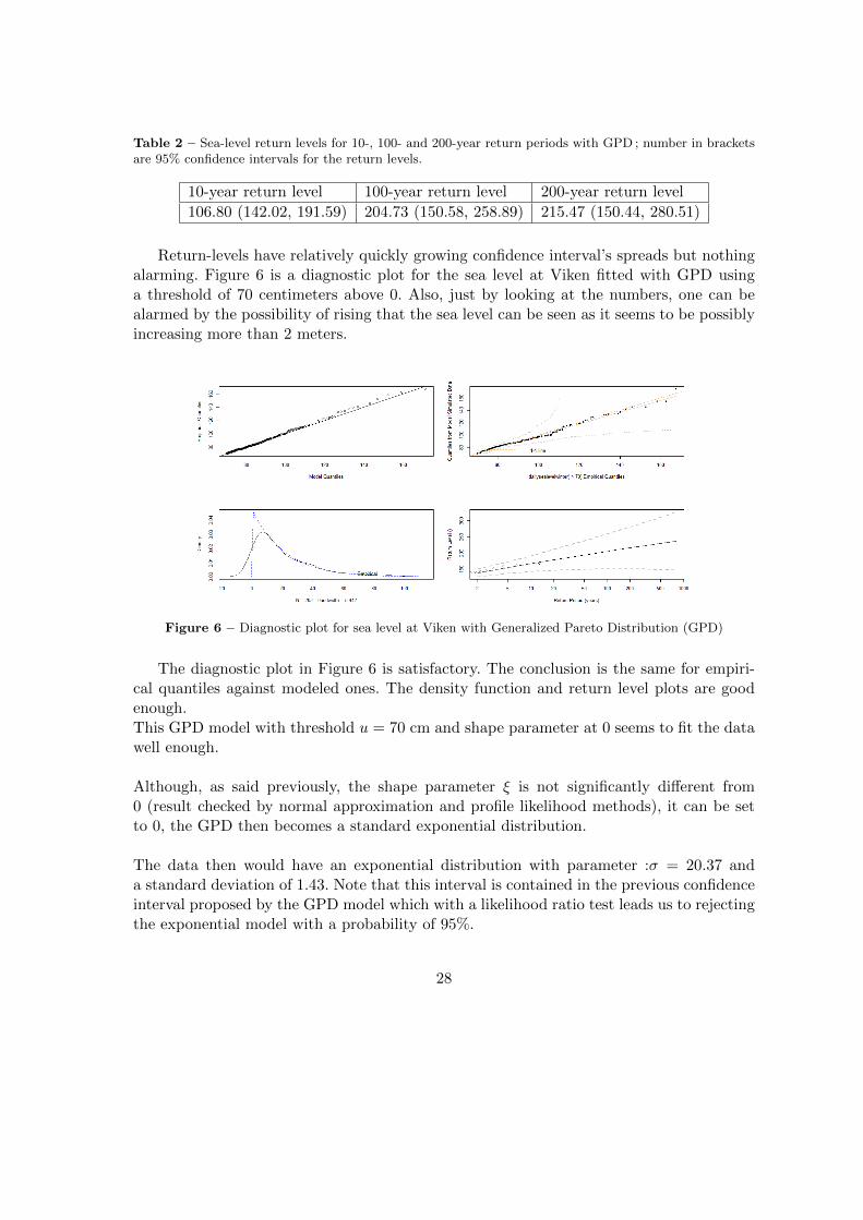
Table 2 – Sea-level return levels for 10-, 100- and 200-year return periods with GPD ; number in bracketsare 95% confidence intervals for the return levels.
10-year return level 100-year return level 200-year return level
106.80 (142.02, 191.59) 204.73 (150.58, 258.89) 215.47 (150.44, 280.51)
Return-levels have relatively quickly growing confidence interval’s spreads but nothingalarming. Figure 6 is a diagnostic plot for the sea level at Viken fitted with GPD usinga threshold of 70 centimeters above 0. Also, just by looking at the numbers, one can bealarmed by the possibility of rising that the sea level can be seen as it seems to be possiblyincreasing more than 2 meters.
Figure 6 – Diagnostic plot for sea level at Viken with Generalized Pareto Distribution (GPD)
The diagnostic plot in Figure 6 is satisfactory. The conclusion is the same for empiri-cal quantiles against modeled ones. The density function and return level plots are goodenough.This GPD model with threshold u = 70 cm and shape parameter at 0 seems to fit the datawell enough.
Although, as said previously, the shape parameter ξ is not significantly different from0 (result checked by normal approximation and profile likelihood methods), it can be setto 0, the GPD then becomes a standard exponential distribution.
The data then would have an exponential distribution with parameter :σ = 20.37 anda standard deviation of 1.43. Note that this interval is contained in the previous confidenceinterval proposed by the GPD model which with a likelihood ratio test leads us to rejectingthe exponential model with a probability of 95%.
28
Later on, in the conclusion part, some interpretation of the results will be done consi-dering flood risks in the bay of Angelholm.
On to maximum run-up
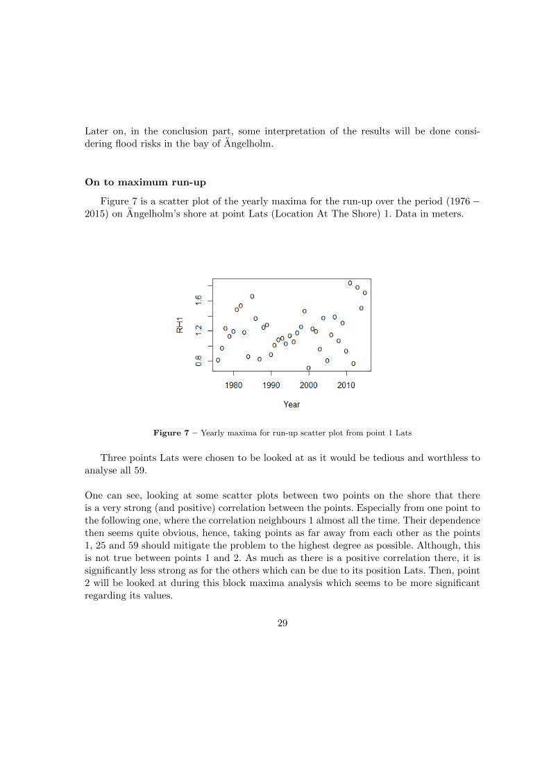
Figure 7 is a scatter plot of the yearly maxima for the run-up over the period (1976−2015) on Angelholm’s shore at point Lats (Location At The Shore) 1. Data in meters.
Figure 7 – Yearly maxima for run-up scatter plot from point 1 Lats
Three points Lats were chosen to be looked at as it would be tedious and worthless toanalyse all 59.
One can see, looking at some scatter plots between two points on the shore that thereis a very strong (and positive) correlation between the points. Especially from one point tothe following one, where the correlation neighbours 1 almost all the time. Their dependencethen seems quite obvious, hence, taking points as far away from each other as the points1, 25 and 59 should mitigate the problem to the highest degree as possible. Although, thisis not true between points 1 and 2. As much as there is a positive correlation there, it issignificantly less strong as for the others which can be due to its position Lats. Then, point2 will be looked at during this block maxima analysis which seems to be more significantregarding its values.
29
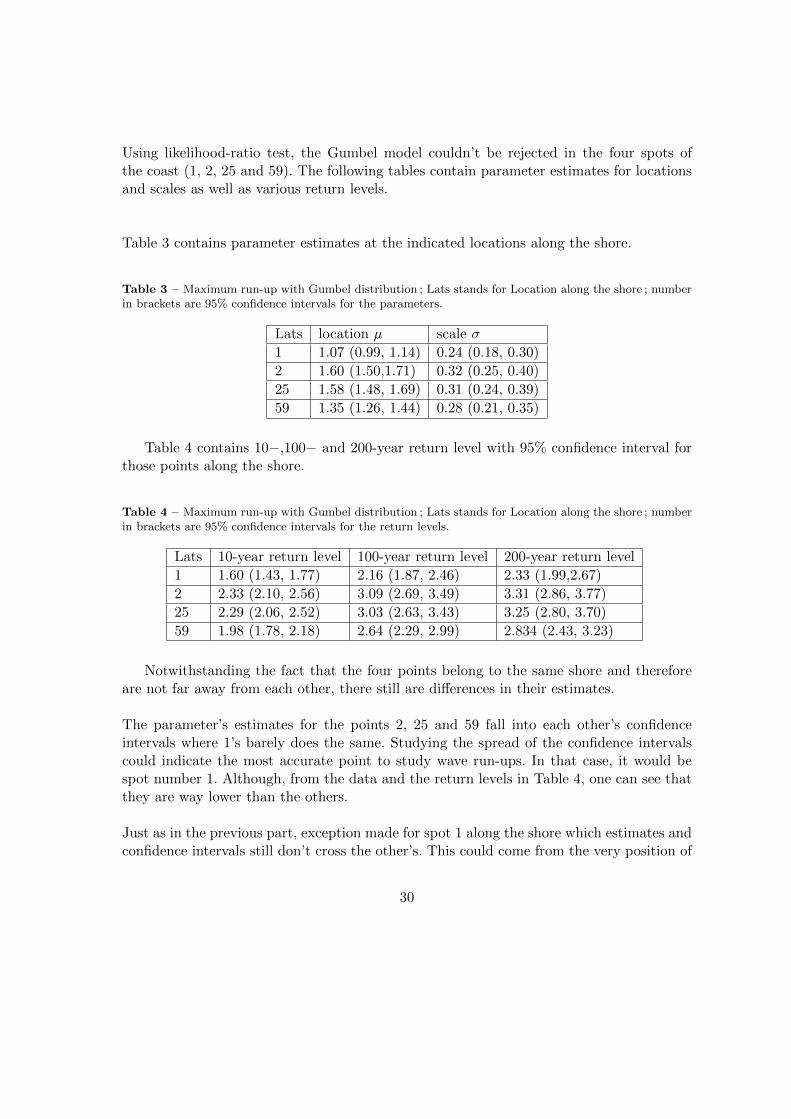
Using likelihood-ratio test, the Gumbel model couldn’t be rejected in the four spots ofthe coast (1, 2, 25 and 59). The following tables contain parameter estimates for locationsand scales as well as various return levels.
Table 3 contains parameter estimates at the indicated locations along the shore.
Table 3 – Maximum run-up with Gumbel distribution ; Lats stands for Location along the shore ; numberin brackets are 95% confidence intervals for the parameters.
Lats location µ scale σ
1 1.07 (0.99, 1.14) 0.24 (0.18, 0.30)
2 1.60 (1.50,1.71) 0.32 (0.25, 0.40)
25 1.58 (1.48, 1.69) 0.31 (0.24, 0.39)
59 1.35 (1.26, 1.44) 0.28 (0.21, 0.35)
Table 4 contains 10−,100− and 200-year return level with 95% confidence interval forthose points along the shore.
Table 4 – Maximum run-up with Gumbel distribution ; Lats stands for Location along the shore ; numberin brackets are 95% confidence intervals for the return levels.
Lats 10-year return level 100-year return level 200-year return level
1 1.60 (1.43, 1.77) 2.16 (1.87, 2.46) 2.33 (1.99,2.67)
2 2.33 (2.10, 2.56) 3.09 (2.69, 3.49) 3.31 (2.86, 3.77)
25 2.29 (2.06, 2.52) 3.03 (2.63, 3.43) 3.25 (2.80, 3.70)
59 1.98 (1.78, 2.18) 2.64 (2.29, 2.99) 2.834 (2.43, 3.23)
Notwithstanding the fact that the four points belong to the same shore and thereforeare not far away from each other, there still are differences in their estimates.
The parameter’s estimates for the points 2, 25 and 59 fall into each other’s confidenceintervals where 1’s barely does the same. Studying the spread of the confidence intervalscould indicate the most accurate point to study wave run-ups. In that case, it would bespot number 1. Although, from the data and the return levels in Table 4, one can see thatthey are way lower than the others.
Just as in the previous part, exception made for spot 1 along the shore which estimates andconfidence intervals still don’t cross the other’s. This could come from the very position of
30
that spot as it is the first one on the shore and may be protected by the shape of the coastitself. Run-ups there seems to be smaller. As the intention is to model the maximum risksof flood on the coast of Angelholm, point 1 should not be taken as the main example there.Dealing with Gumbel distribution (shape ξ = 0), the MLE of the upper end-point is infinity.
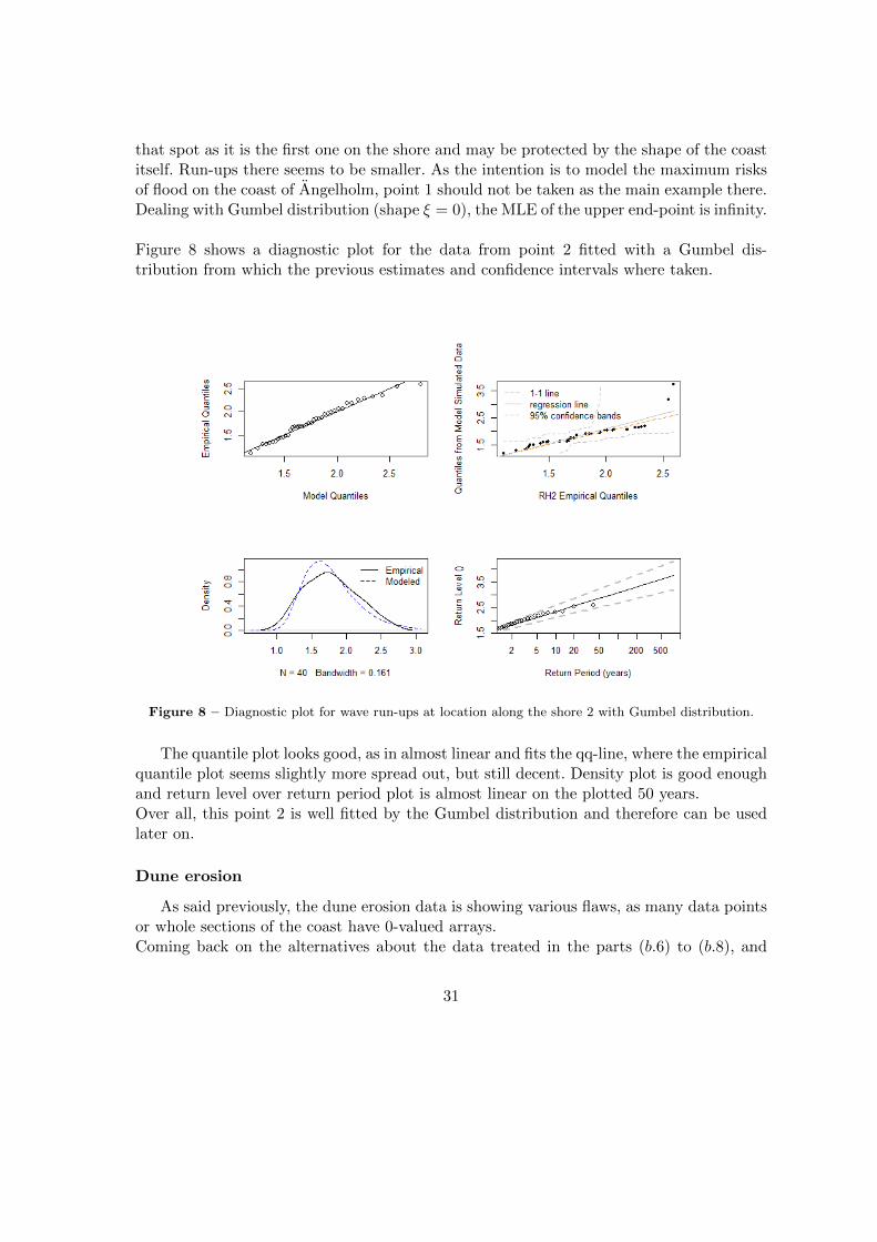
Figure 8 shows a diagnostic plot for the data from point 2 fitted with a Gumbel dis-tribution from which the previous estimates and confidence intervals where taken.
Figure 8 – Diagnostic plot for wave run-ups at location along the shore 2 with Gumbel distribution.
The quantile plot looks good, as in almost linear and fits the qq-line, where the empiricalquantile plot seems slightly more spread out, but still decent. Density plot is good enoughand return level over return period plot is almost linear on the plotted 50 years.Over all, this point 2 is well fitted by the Gumbel distribution and therefore can be usedlater on.
Dune erosion
As said previously, the dune erosion data is showing various flaws, as many data pointsor whole sections of the coast have 0-valued arrays.Coming back on the alternatives about the data treated in the parts (b.6) to (b.8), and
31
using two years as a block size for running block maxima on the sets it shows identicalresults using either alternative (b.7), the maxima over the 3 main neighbouring spots Latsor (b.8), the maxima over the whole bay as the maxima over the vay and over those 3 spotsare the same.
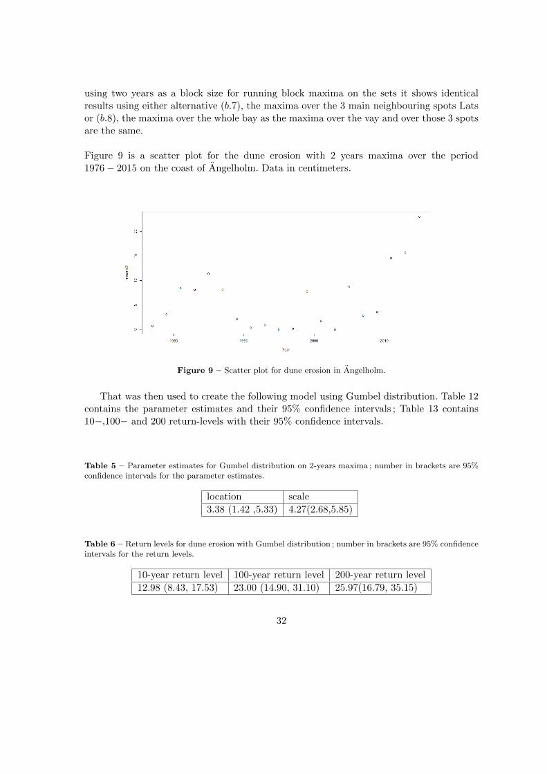
Figure 9 is a scatter plot for the dune erosion with 2 years maxima over the period1976− 2015 on the coast of Angelholm. Data in centimeters.
Figure 9 – Scatter plot for dune erosion in Angelholm.
That was then used to create the following model using Gumbel distribution. Table 12contains the parameter estimates and their 95% confidence intervals ; Table 13 contains10−,100− and 200 return-levels with their 95% confidence intervals.
Table 5 – Parameter estimates for Gumbel distribution on 2-years maxima ; number in brackets are 95%confidence intervals for the parameter estimates.
location scale
3.38 (1.42 ,5.33) 4.27(2.68,5.85)
Table 6 – Return levels for dune erosion with Gumbel distribution ; number in brackets are 95% confidenceintervals for the return levels.
10-year return level 100-year return level 200-year return level
12.98 (8.43, 17.53) 23.00 (14.90, 31.10) 25.97(16.79, 35.15)
32
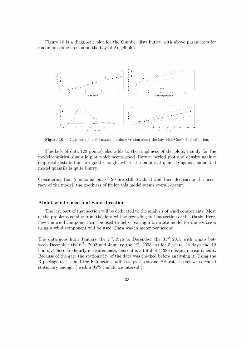
Figure 10 is a diagnostic plot for the Gumbel distribution with above parameters formaximum dune erosion on the bay of Angelholm.
Figure 10 – Diagnostic plot for maximum dune erosion along the bay with Gumbel distribution.
The lack of data (20 points) also adds to the roughness of the plots, mainly for themodel/empirical quantile plot which seems good. Return period plot and density againstempirical distribution are good enough, where the empirical quantile against simulatedmodel quantile is quite blurry.
Considering that 2 maxima out of 20 are still 0-valued and then decreasing the accu-racy of the model, the goodness of fit for this model seems overall decent.
About wind speed and wind direction
The last part of that section will be dedicated to the analysis of wind components. Mostof the problems coming from the data will be regarding to that section of this thesis. Here,how the wind component can be used to help creating a bivariate model for dune erosionusing a wind component will be used. Data was in meter per second.
The data goes from January the 1st, 1976 to December the 31st, 2015 with a gap bet-ween December the 6th, 2002 and January the 1st, 2008 (so for 5 years, 24 days and 12hours). Those are hourly measurements, hence it is a total of 44388 missing measurements.Because of the gap, the stationarity of the data was checked before analysing it. Using theR-package tseries and the R functions adf.test, pkss.test and PP.test, the set was deemedstationary enough ( with a 95% confidence interval ).
33
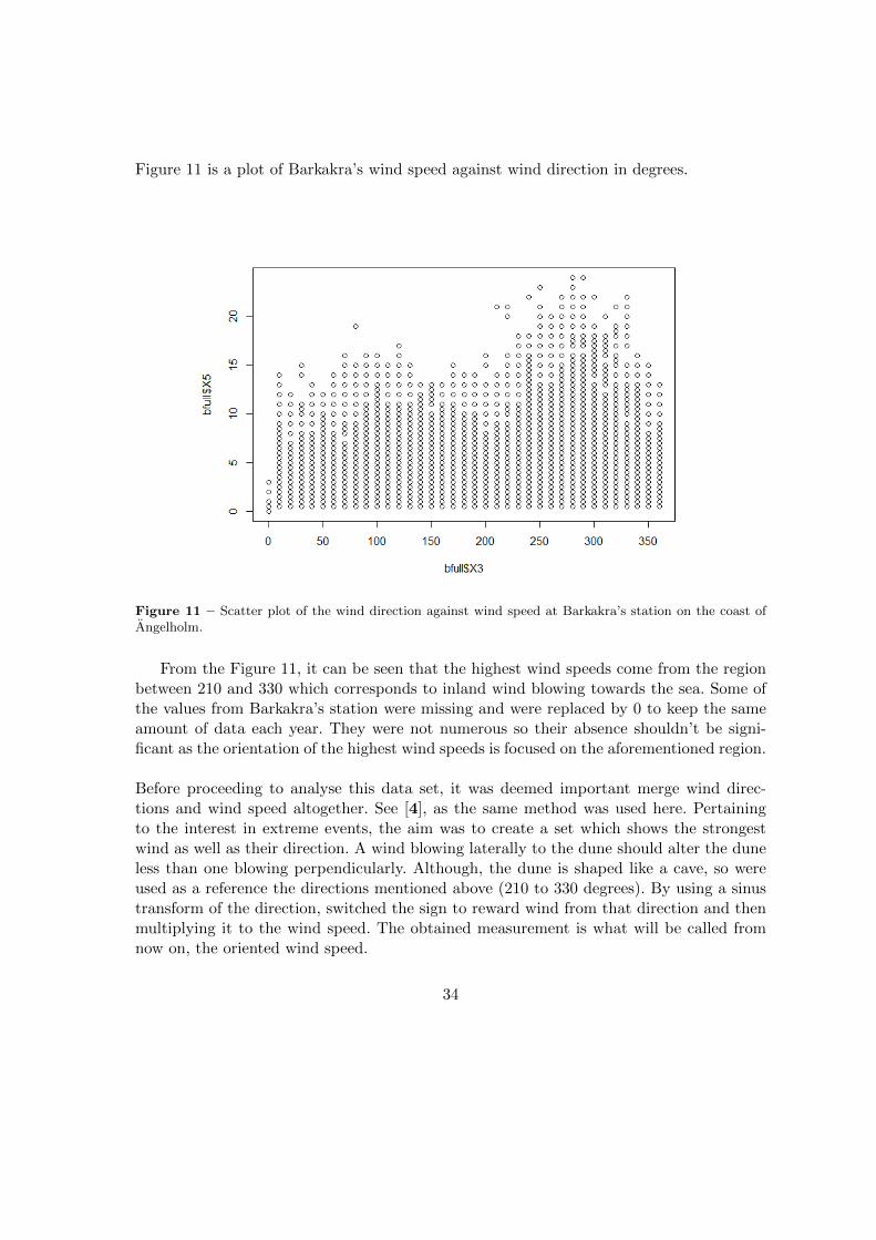
Figure 11 is a plot of Barkakra’s wind speed against wind direction in degrees.
Figure 11 – Scatter plot of the wind direction against wind speed at Barkakra’s station on the coast ofAngelholm.
From the Figure 11, it can be seen that the highest wind speeds come from the regionbetween 210 and 330 which corresponds to inland wind blowing towards the sea. Some ofthe values from Barkakra’s station were missing and were replaced by 0 to keep the sameamount of data each year. They were not numerous so their absence shouldn’t be signi-ficant as the orientation of the highest wind speeds is focused on the aforementioned region.
Before proceeding to analyse this data set, it was deemed important merge wind direc-tions and wind speed altogether. See [4], as the same method was used here. Pertainingto the interest in extreme events, the aim was to create a set which shows the strongestwind as well as their direction. A wind blowing laterally to the dune should alter the duneless than one blowing perpendicularly. Although, the dune is shaped like a cave, so wereused as a reference the directions mentioned above (210 to 330 degrees). By using a sinustransform of the direction, switched the sign to reward wind from that direction and thenmultiplying it to the wind speed. The obtained measurement is what will be called fromnow on, the oriented wind speed.
34
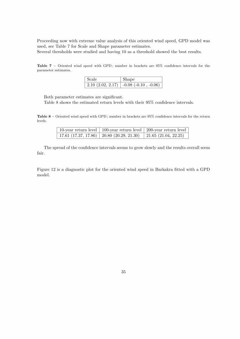
Proceeding now with extreme value analysis of this oriented wind speed, GPD model wasused, see Table 7 for Scale and Shape parameter estimates.Several thresholds were studied and having 10 as a threshold showed the best results.
Table 7 – Oriented wind speed with GPD ; number in brackets are 95% confidence intervals for theparameter estimates.
Scale Shape
2.10 (2.02, 2.17) -0.08 (-0.10 , -0.06)
Both parameter estimates are significant.Table 8 shows the estimated return levels with their 95% confidence intervals.
Table 8 – Oriented wind speed with GPD ; number in brackets are 95% confidence intervals for the returnlevels.
10-year return level 100-year return level 200-year return level
17.61 (17.37, 17.86) 20.80 (20.29, 21.30) 21.65 (21.04, 22.25)
The spread of the confidence intervals seems to grow slowly and the results overall seemfair.
Figure 12 is a diagnostic plot for the oriented wind speed in Barkakra fitted with a GPDmodel.
35
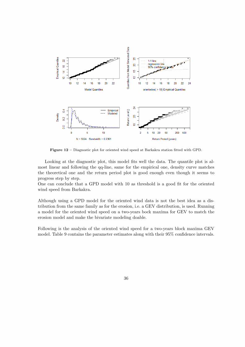
Figure 12 – Diagnostic plot for oriented wind speed at Barkakra station fitted with GPD.
Looking at the diagnostic plot, this model fits well the data. The quantile plot is al-most linear and following the qq-line, same for the empirical one, density curve matchesthe theoretical one and the return period plot is good enough even though it seems toprogress step by step.One can conclude that a GPD model with 10 as threshold is a good fit for the orientedwind speed from Barkakra.
Although using a GPD model for the oriented wind data is not the best idea as a dis-tribution from the same family as for the erosion, i.e. a GEV distribution, is used. Runninga model for the oriented wind speed on a two-years bock maxima for GEV to match theerosion model and make the bivariate modeling doable.
Following is the analysis of the oriented wind speed for a two-years block maxima GEVmodel. Table 9 contains the parameter estimates along with their 95% confidence intervals.
36
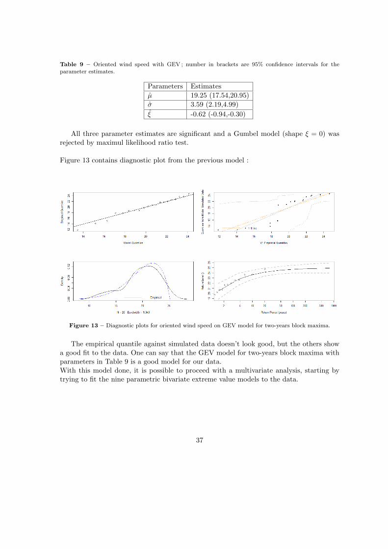
Table 9 – Oriented wind speed with GEV ; number in brackets are 95% confidence intervals for theparameter estimates.
Parameters Estimates
µ 19.25 (17.54,20.95)
σ 3.59 (2.19,4.99)
ξ -0.62 (-0.94,-0.30)
All three parameter estimates are significant and a Gumbel model (shape ξ = 0) wasrejected by maximul likelihood ratio test.
Figure 13 contains diagnostic plot from the previous model :
Figure 13 – Diagnostic plots for oriented wind speed on GEV model for two-years block maxima.
The empirical quantile against simulated data doesn’t look good, but the others showa good fit to the data. One can say that the GEV model for two-years block maxima withparameters in Table 9 is a good model for our data.With this model done, it is possible to proceed with a multivariate analysis, starting bytrying to fit the nine parametric bivariate extreme value models to the data.
37
4.2 Multivariate analysis
As said previously, the main topic of this thesis is to model the effect of the wind ondune erosion. To do so, one wants to use a bivariate extreme value model. Because of theerosion data available (i.e. yearly maxima), only a bivariate block maxima can be fitted.Some information about the wind : the oriented wind speed is, as explained earlier, a com-bination of the speed and the direction of the wind, data from Barkakra station next tothe shore of Angelholm.
About the yearly erosion, and, as explained earlier : Most of the data points actuallyare 0’s, making any analysis very difficult. Some spots Lats still have a lot of zeros or arecompletely zeros and therefore won’t be used. They are mainly the points from 27 Lats to59 Lats.The amount of 0-valued points in the set was reduced by taking twice as large block maxima(i.e. from one year to two years block size). This is alternative (b.8). Even though half theoriginal data size is rather low, the values now make more sense. Then, looking at whatwas left, and because of the interest in maximal values, it is required to choose data thatis high enough for the analysis.
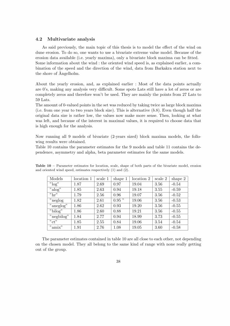
Now running all 9 models of bivariate (2-years sized) block maxima models, the follo-wing results were obtained.Table 10 contains the parameter estimates for the 9 models and table 11 contains the de-pendence, asymmetry and alpha, beta parameter estimates for the same models.
Table 10 – Parameter estimates for location, scale, shape of both parts of the bivariate model, erosionand oriented wind speed, estimates respectively (1) and (2).
Models location 1 scale 1 shape 1 location 2 scale 2 shape 2
”log” 1.87 2.69 0.97 19.04 3.56 -0.54
”alog” 1.85 2.63 0.94 19.18 3.55 -0.59
”hr” 1.79 2.56 0.96 19.07 3.56 -0.52
”neglog 1.82 2.61 0.95 ” 19.06 3.56 -0.53
”aneglog” 1.86 2.62 0.93 19.20 3.56 -0.55
”bilog” 1.86 2.60 0.88 19.21 3.56 -0.55
”negbilog” 1.84 2.77 0.94 18.99 3.73 -0.55
”ct” 1.85 2.55 0.84 19.06 3.54 -0.54
”amix” 1.91 2.76 1.08 19.05 3.60 -0.58
The parameter estimates contained in table 10 are all close to each other, not dependingon the chosen model. They all belong to the same kind of range with none really gettingout of the group.
38
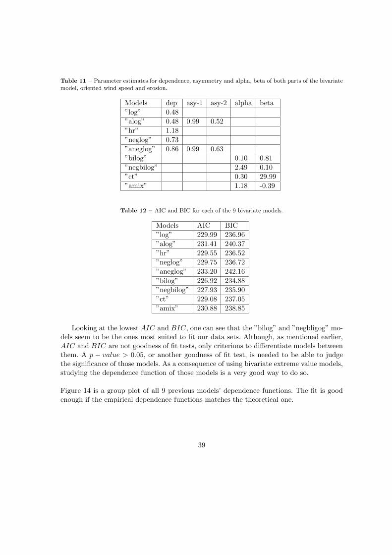
Table 11 – Parameter estimates for dependence, asymmetry and alpha, beta of both parts of the bivariatemodel, oriented wind speed and erosion.
Models dep asy-1 asy-2 alpha beta
”log” 0.48
”alog” 0.48 0.99 0.52
”hr” 1.18
”neglog” 0.73
”aneglog” 0.86 0.99 0.63
”bilog” 0.10 0.81
”negbilog” 2.49 0.10
”ct” 0.30 29.99
”amix” 1.18 -0.39
Table 12 – AIC and BIC for each of the 9 bivariate models.
Models AIC BIC
”log” 229.99 236.96
”alog” 231.41 240.37
”hr” 229.55 236.52
”neglog” 229.75 236.72
”aneglog” 233.20 242.16
”bilog” 226.92 234.88
”negbilog” 227.93 235.90
”ct” 229.08 237.05
”amix” 230.88 238.85
Looking at the lowest AIC and BIC, one can see that the ”bilog” and ”negbligog” mo-dels seem to be the ones most suited to fit our data sets. Although, as mentioned earlier,AIC and BIC are not goodness of fit tests, only criterions to differentiate models betweenthem. A p − value > 0.05, or another goodness of fit test, is needed to be able to judgethe significance of those models. As a consequence of using bivariate extreme value models,studying the dependence function of those models is a very good way to do so.
Figure 14 is a group plot of all 9 previous models’ dependence functions. The fit is goodenough if the empirical dependence functions matches the theoretical one.
39
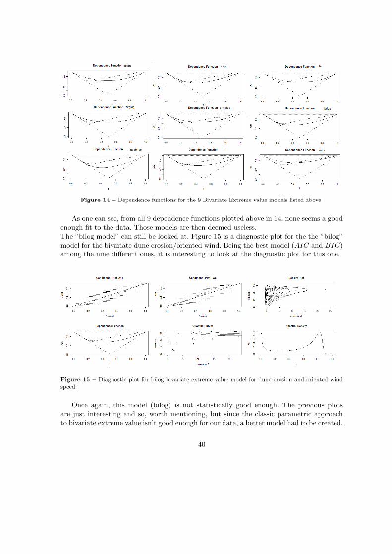
Figure 14 – Dependence functions for the 9 Bivariate Extreme value models listed above.
As one can see, from all 9 dependence functions plotted above in 14, none seems a goodenough fit to the data. Those models are then deemed useless.The ”bilog model” can still be looked at. Figure 15 is a diagnostic plot for the the ”bilog”model for the bivariate dune erosion/oriented wind. Being the best model (AIC and BIC)among the nine different ones, it is interesting to look at the diagnostic plot for this one.
Figure 15 – Diagnostic plot for bilog bivariate extreme value model for dune erosion and oriented windspeed.
Once again, this model (bilog) is not statistically good enough. The previous plotsare just interesting and so, worth mentioning, but since the classic parametric approachto bivariate extreme value isn’t good enough for our data, a better model had to be created.
40
4.3 Copula estimation of bivariate extreme value model
As well as trying this new approach using copulas, the same data set as in the univariateanalysis was used, i.e. a two-years block maxima for the oriented wind speed and on thewhole coast erosion.
Using the marginal distributions for both erosion and oriented wind speed, respectivelyGumbel and GEV distributions,the data set was transformed into a set of uniform U [0, 1]2
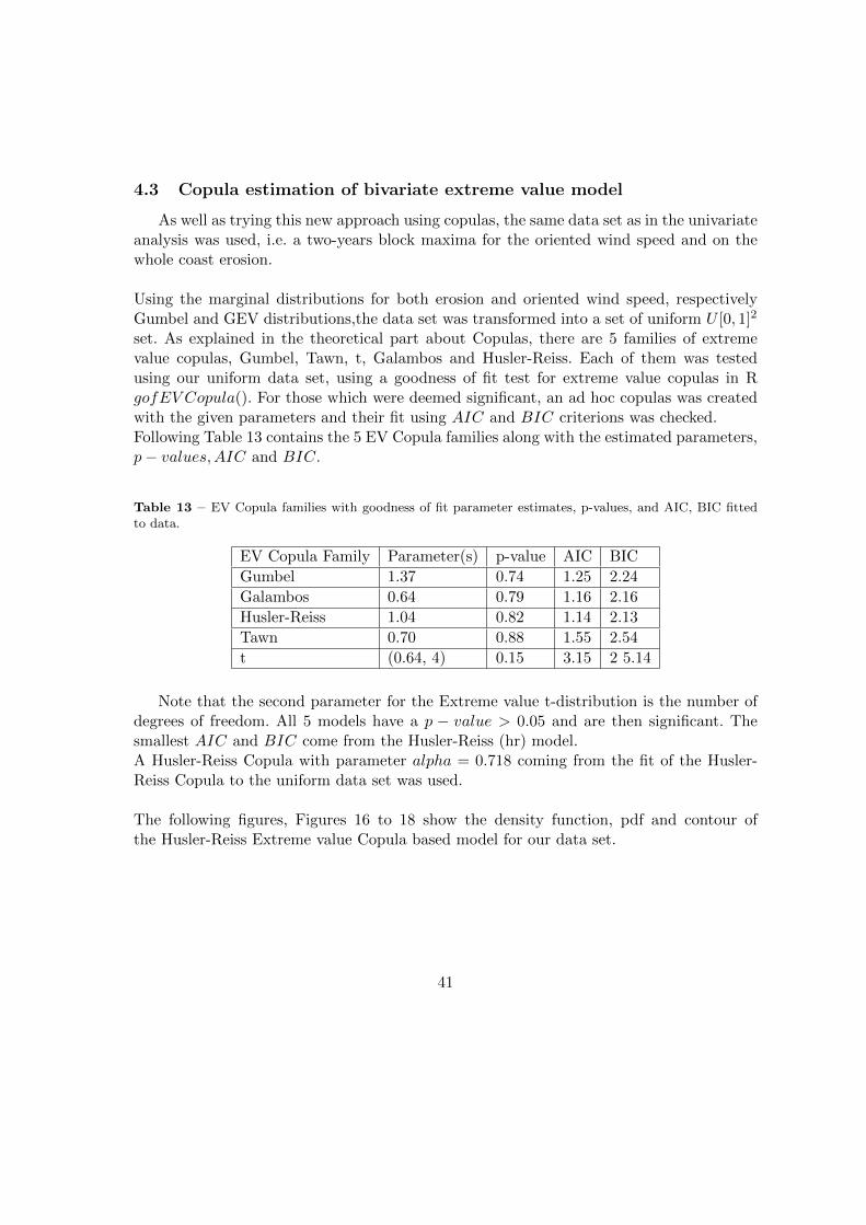
set. As explained in the theoretical part about Copulas, there are 5 families of extremevalue copulas, Gumbel, Tawn, t, Galambos and Husler-Reiss. Each of them was testedusing our uniform data set, using a goodness of fit test for extreme value copulas in RgofEV Copula(). For those which were deemed significant, an ad hoc copulas was createdwith the given parameters and their fit using AIC and BIC criterions was checked.Following Table 13 contains the 5 EV Copula families along with the estimated parameters,p− values,AIC and BIC.
Table 13 – EV Copula families with goodness of fit parameter estimates, p-values, and AIC, BIC fittedto data.
EV Copula Family Parameter(s) p-value AIC BIC
Gumbel 1.37 0.74 1.25 2.24
Galambos 0.64 0.79 1.16 2.16
Husler-Reiss 1.04 0.82 1.14 2.13
Tawn 0.70 0.88 1.55 2.54
t (0.64, 4) 0.15 3.15 2 5.14
Note that the second parameter for the Extreme value t-distribution is the number ofdegrees of freedom. All 5 models have a p − value > 0.05 and are then significant. Thesmallest AIC and BIC come from the Husler-Reiss (hr) model.A Husler-Reiss Copula with parameter alpha = 0.718 coming from the fit of the Husler-Reiss Copula to the uniform data set was used.
The following figures, Figures 16 to 18 show the density function, pdf and contour ofthe Husler-Reiss Extreme value Copula based model for our data set.
41
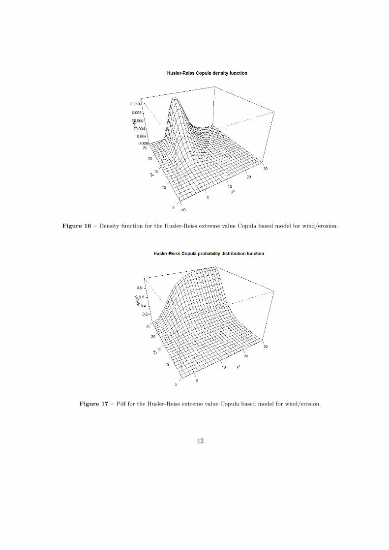
Figure 16 – Density function for the Husler-Reiss extreme value Copula based model for wind/erosion.
Figure 17 – Pdf for the Husler-Reiss extreme value Copula based model for wind/erosion.
42
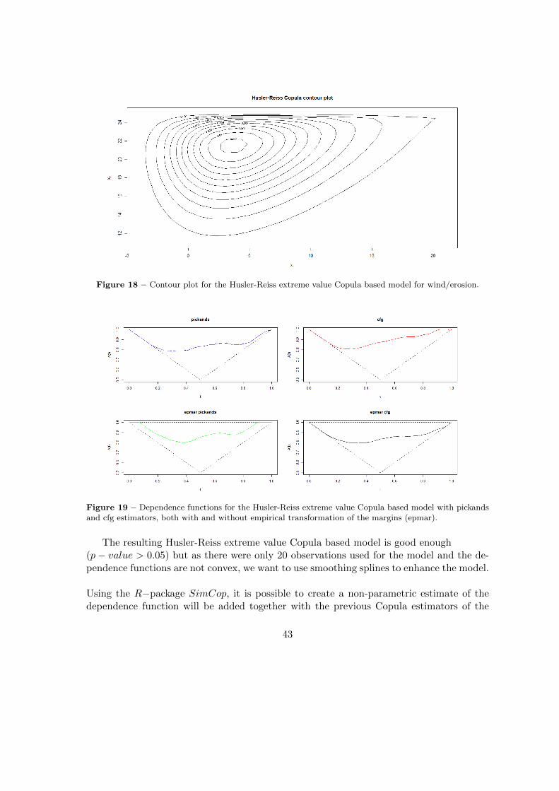
Figure 18 – Contour plot for the Husler-Reiss extreme value Copula based model for wind/erosion.
Figure 19 – Dependence functions for the Husler-Reiss extreme value Copula based model with pickandsand cfg estimators, both with and without empirical transformation of the margins (epmar).
The resulting Husler-Reiss extreme value Copula based model is good enough(p− value > 0.05) but as there were only 20 observations used for the model and the de-pendence functions are not convex, we want to use smoothing splines to enhance the model.
Using the R−package SimCop, it is possible to create a non-parametric estimate of thedependence function will be added together with the previous Copula estimators of the
43
dependence function.
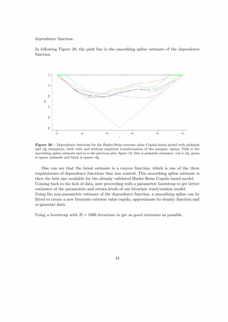
In following Figure 20, the pink line is the smoothing spline estimate of the dependencefunction.
Figure 20 – Dependence functions for the Husler-Reiss extreme value Copula based model with pickandsand cfg estimators, both with and without empirical transformation of the margins, epmar. Pink is thesmoothing spline estimate and as is the previous plot, figure 19, blue is pickands estimator, red is cfg, greenis epmar pickands and black is epmar cfg.
One can see that the latest estimate is a convex function, which is one of the threerequirements of dependence functions that was wanted. This smoothing spline estimate isthen the best one available for the already validated Husler-Reiss Copula based model.Coming back to the lack of data, now proceeding with a parametric bootstrap to get betterestimates of the parameters and return-levels of our bivariate wind/erosion model.Using the non-parametric estimate of the dependence function, a smoothing spline can befitted to create a new bivariate extreme value copula, approximate its density function andre-generate data.
Using a bootstrap with B = 1000 iterations to get as good estimates as possible.
44
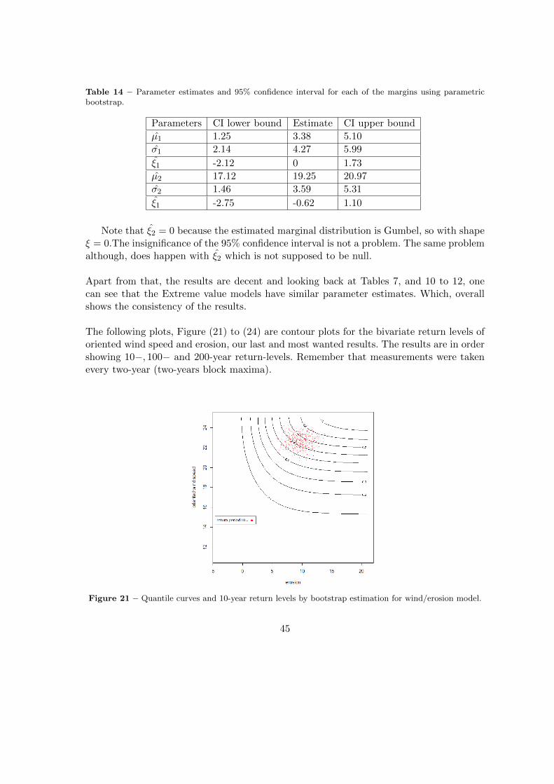
Table 14 – Parameter estimates and 95% confidence interval for each of the margins using parametricbootstrap.
Parameters CI lower bound Estimate CI upper bound
µ1 1.25 3.38 5.10
σ1 2.14 4.27 5.99
ξ1 -2.12 0 1.73
µ2 17.12 19.25 20.97
σ2 1.46 3.59 5.31
ξ1 -2.75 -0.62 1.10
Note that ξ2 = 0 because the estimated marginal distribution is Gumbel, so with shapeξ = 0.The insignificance of the 95% confidence interval is not a problem. The same problemalthough, does happen with ξ2 which is not supposed to be null.
Apart from that, the results are decent and looking back at Tables 7, and 10 to 12, onecan see that the Extreme value models have similar parameter estimates. Which, overallshows the consistency of the results.
The following plots, Figure (21) to (24) are contour plots for the bivariate return levels oforiented wind speed and erosion, our last and most wanted results. The results are in ordershowing 10−, 100− and 200-year return-levels. Remember that measurements were takenevery two-year (two-years block maxima).
Figure 21 – Quantile curves and 10-year return levels by bootstrap estimation for wind/erosion model.
45
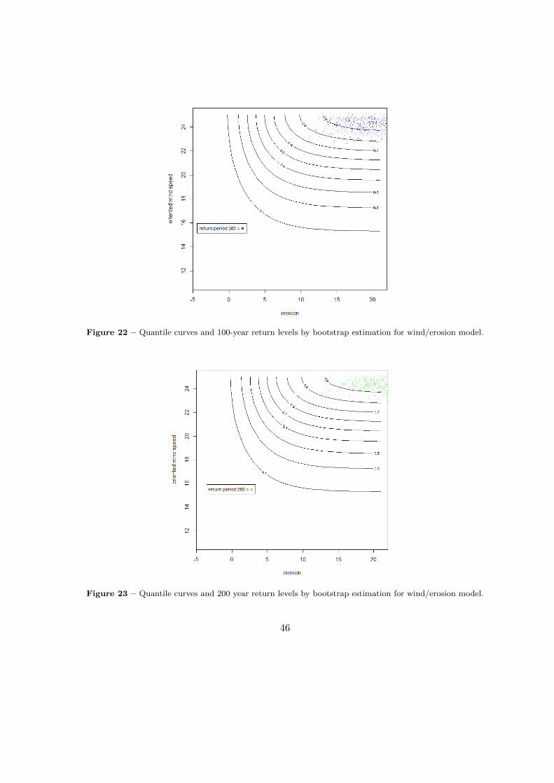
Figure 22 – Quantile curves and 100-year return levels by bootstrap estimation for wind/erosion model.
Figure 23 – Quantile curves and 200 year return levels by bootstrap estimation for wind/erosion model.
46
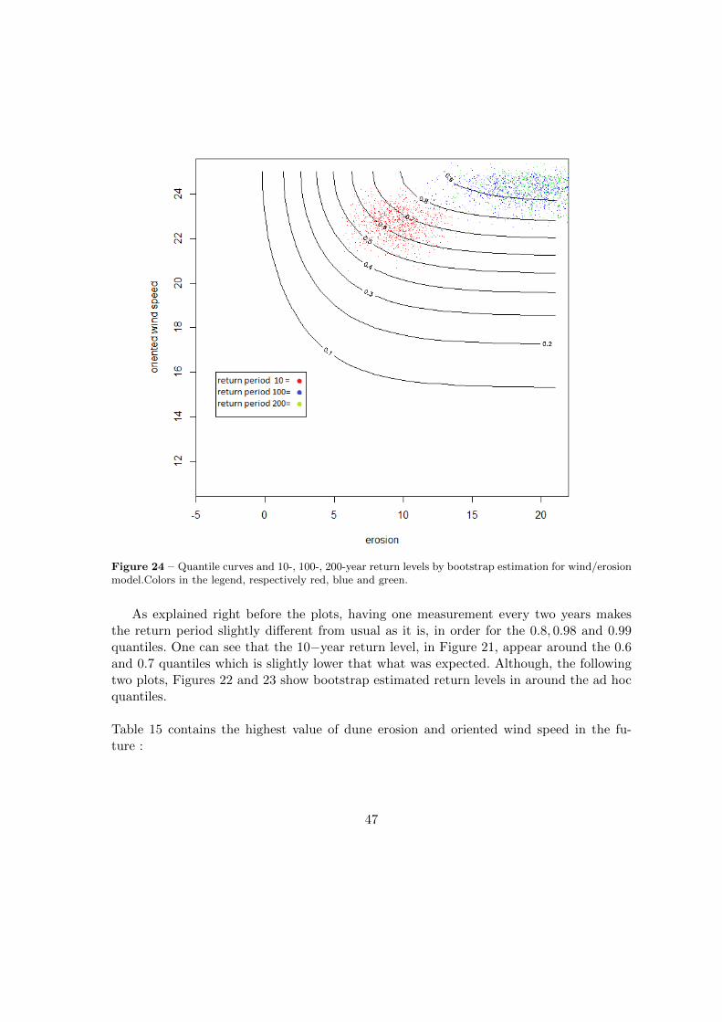
Figure 24 – Quantile curves and 10-, 100-, 200-year return levels by bootstrap estimation for wind/erosionmodel.Colors in the legend, respectively red, blue and green.
As explained right before the plots, having one measurement every two years makesthe return period slightly different from usual as it is, in order for the 0.8, 0.98 and 0.99quantiles. One can see that the 10−year return level, in Figure 21, appear around the 0.6and 0.7 quantiles which is slightly lower that what was expected. Although, the followingtwo plots, Figures 22 and 23 show bootstrap estimated return levels in around the ad hocquantiles.
Table 15 contains the highest value of dune erosion and oriented wind speed in the fu-ture :
47
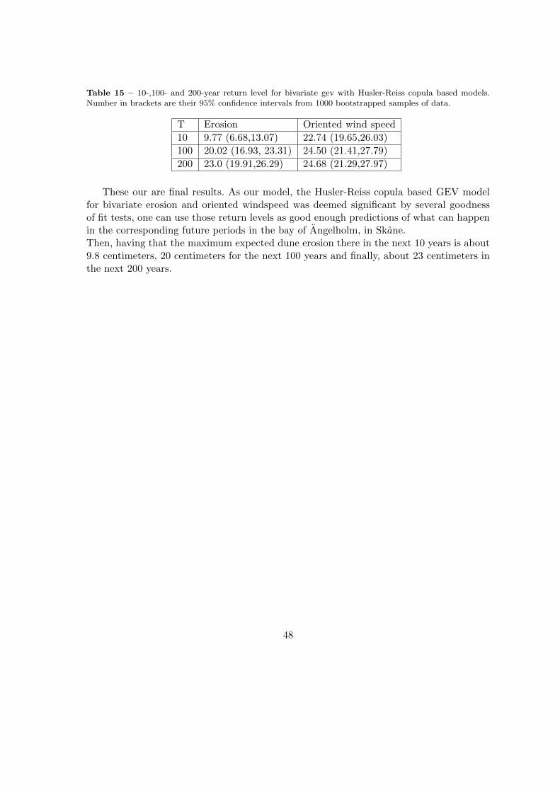
Table 15 – 10-,100- and 200-year return level for bivariate gev with Husler-Reiss copula based models.Number in brackets are their 95% confidence intervals from 1000 bootstrapped samples of data.
T Erosion Oriented wind speed
10 9.77 (6.68,13.07) 22.74 (19.65,26.03)
100 20.02 (16.93, 23.31) 24.50 (21.41,27.79)
200 23.0 (19.91,26.29) 24.68 (21.29,27.97)
These our are final results. As our model, the Husler-Reiss copula based GEV modelfor bivariate erosion and oriented windspeed was deemed significant by several goodnessof fit tests, one can use those return levels as good enough predictions of what can happenin the corresponding future periods in the bay of Angelholm, in Skane.Then, having that the maximum expected dune erosion there in the next 10 years is about9.8 centimeters, 20 centimeters for the next 100 years and finally, about 23 centimeters inthe next 200 years.
48
5 Conclusions, discussions and possible improvements.
The dune erosion level is an indicator of climate anthropy and can be used for flood risksprevision. In this report, several analysis were performed around the idea of such previsionsbut were mostly focused on a bivariate model between the dune erosion and wind speed.The dune erosion on the shore of Angelholm’s data, provided from 1976 to 2015, was on ayearly maxima format and thus, wind speed data needed to be cut down to this format aswell. Using extreme-value theory, several models were fitted to the data to try and explainhow each phenomena was behaving. Using block maxima on sea-level , wave runup, duneerosion and oriented wind speed with 1, 1, 2 and 2 years blocks respectively. Afterwards, amodel fitting both dune erosion and wind speed was created. Because of a lack of goodnessof fit, copula theory was used to get a better model, using Husler-Reiss’s bivariate extremevalue copula. From the latter, several interesting return levels were calculated along withtheir confidence intervals using smoothing splines and boostrap method, giving an idea ofhow much erosion the dunes in Angelholm would get in the future as well as the highestwind speeds the area would get.The The analysis of the effect of wind on dune erosion in the bay of Angelholm is now donewith a significant model and return levels were calculated for three interesting periods oftime.The Husler-Reiss Copula-based Bivariate Extreme value model for oriented wind speedand dune erosion, helped by bootstrapping and smoothing splines means gave us estimatesthat can be used to avoid damages in the bay for the future times.
Referring to the diagram 2 with the dune, dune erosion, sea-water level and wave runup,one can now use the calculations made during the analysis of all those data sets.Keep in mind that this part is not the main topic of this thesis but is here to show howto use almost directly the results from the bivariate model of the effect of wind on duneerosion. The calculations here will be kept simple. By using the 95% quantile of the extremevalues distributions one can, by plain sums, get the following results :
118.91 centimeters for a 10-year period ;227.84 centimeters for a 100-year period ;and 241.861 centimeters for a 200-year period, which is the height of the coastal protectionsneeded in the bay of Angelholm in Skane to avoid flooding in the future.
Remember that this part is just a simple calculation that is not made to be used straightaway. The mere point of those is to show that the dune erosion, even though it representsa small part of those numbers is still important and thus should not be neglected.
Studying all of the 59 points located along the shore would not have given more in-sight or better results about the global effect of the wind on dune erosion on the coast of
49
Angelholm, as it would mean running 59 analysis, which is a lot and seems like a ratherinefficient way of analysing the data there.Also, for the erosion, most of the points Lats have a nearly 0-valued data set, which is whya whole-coast-set was used instead of a single point. There is no use studying the pointsindependently.
A way to get around the gap in Barkakra’s data set would have been to reconstructthe missing values using more advanced techniques, such as, for example, a Kalman filter(alternative b.5). A Kalman filter is the exact solution of a state filtering problem for lineardynamic models ; see [6], p.289. Kalman filters usually needs data with assumptions aboutlinearity and normality but according to [6] in appendix A, p.332, it can be shown, usingHilbert space formalism that these predictions, and updates, are the optimal linear updates,even when the distributions are non-Gaussian. Although, for this thesis, it was deemed un-necessary and rather tedious, considering that the reconstruction using Hallands Vadero Astation’s data was good enough. Reconstructing two points was worthless.With more time, it would be interesting to study the following points or topics :
— gathering more data on dune erosion and dune height to make more accurate modelswhere a reconstruction would then be useful ;
— looking into the SMHI models for their unverified data, it would then be possibleto use only the verified points or the whole set with more insight of their meaning ;
— trying to model other climatic phenomenon with the erosion to see if there havemore impact on it than the wind.
50
Bibliographie
I would like to thank the authors of the following books, articles, thesis, packagesand documents which helped me along the way in my own thesis :
[1] S. Coles (2001), ”An introduction to statistical modeling of extreme va-lues” ;
[2] R.B. Nelsen (2006) ; ”An introduction to copulas”
[3] C. Hallin (2019), ”Long-term beach and dune evolution, Developmentand application of the CS-model” ;
[4] K. Persson (2017), ”On risk analysis of extreme sea levels in Falsterbopeninsula” ;
[5] C. Maia (2010), ”Multivariate Empirical Cumulative Distribution Func-tions”, code and package ;
[6] H. Madsen, E. Lindstrm, J.N Nielsen (2015), ”Statistics for finance” ;
[7] A. Jakobsson (2016), ”An introduction to time series modeling” ;
[8] M. Sandsten, G. Lindgren, H. Rootzn (2014), ”Stationary stochastic pro-cesses for scientists and engineers” ;
51