F – 1 Copyright © 2010 Pearson Education, Inc. Publishing as Prentice Hall. Financial Analysis F For Operations Management, 9e by Krajewski/Ritzman/Malhotra

F – 1Copyright © 2010 Pearson Education, Inc. Publishing as Prentice Hall.

Financial AnalysisFinancial AnalysisF

For For Operations Management, 9eOperations Management, 9e by by Krajewski/Ritzman/Malhotra Krajewski/Ritzman/Malhotra © 2010 Pearson Education© 2010 Pearson Education

PowerPoint Slides PowerPoint Slides by Jeff Heylby Jeff Heyl


Time Value of Money Time Value of Money

Future value of an investment Compounded interest The value of an investment at the end of the period Requires all values be in the same units of time

The value of a $5,000 investment at 12 percent per year, 1 year from now is

$5,000(1.12) = $5,600

If the entire amount remains invested, at the end of 2 years you would have

$5,600(1.12) = $5,000(1.12)2 = $6,272


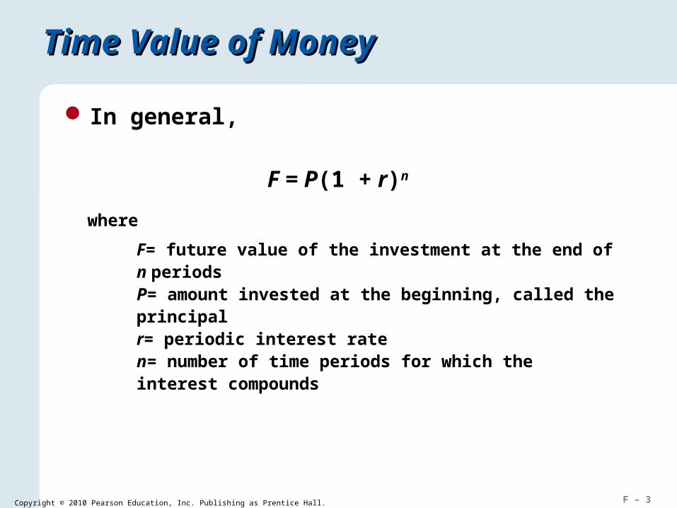
F = P(1 + r)n

where

F= future value of the investment at the end of n periodsP= amount invested at the beginning, called the principalr= periodic interest raten= number of time periods for which the interest compounds

Time Value of Money Time Value of Money

In general,


500(1 + .06)5 = 500(1.338) = $669.11

Application F.1Application F.1

Future Value of a $500 Investment in 5 Years

P= $500r= 6%n= 5

F= P(1 + r)n

SOLUTION


Present Value of a Future AmountPresent Value of a Future Amount

The amount that must be invested now to accumulate to a certain amount in future at a specified interest rate

Discounting is the process of finding the present value of an investment when the future value and the interest rate are known

An investment worth $10,000 at the end of 1 year if the interest rate is 12 percent

F = $10,000 = P(1 + 0.12)

nr

FP

1 9298$

1201

000101 ,

.

,


where

F= future value of the investment at the end of n periodsP= amount invested at the beginning, called the principalr= periodic interest rate (discount rate)n= number of time periods for which the interest compounds

P =F

(1 + r)n

Present Value of a Future AmountPresent Value of a Future Amount

In general,

The interest rate is also called the discount rate


$500/1.338 = $373.63


P =F

(1 + r)n

F= $500r= 6%n= 5

Present Value of $500 Received in Five Years

SOLUTION


[1/(1 + r)n] is the present value factor (pf)

Found in Table F.1

Present Value FactorsPresent Value Factors

The present value of a future amount

nn rF

r

FP

1

1

1



TABLE F.1 | PRESENT VALUE FACTORS FOR A SINGLE PAYMENT (Partial)

Number of Periods (n)

Interest Rate (r)

0.01 0.02 0.03 0.04 0.05 0.06 0.08 0.10 0.12 0.14

1 0.9901 0.9804 0.9709 0.9615 0.9524 0.9434 0.9259 0.9091 0.8929 0.8772

2 0.9803 0.9612 0.9426 0.9246 0.9070 0.8900 0.8573 0.8264 0.7972 0.7695

3 0.9706 0.9423 0.9151 0.8890 0.8638 0.8396 0.7938 0.7513 0.7118 0.6750

4 0.9610 0.9238 0.8885 0.8548 0.8227 0.7921 0.7350 0.6830 0.6355 0.5921

5 0.9515 0.9057 0.8626 0.8219 0.7835 0.7473 0.6806 0.6209 0.5674 0.4194

6 0.9420 0.8880 0.8375 0.7903 0.7462 0.7050 0.6302 0.5645 0.5066 0.4556

7 0.9327 0.8706 0.8131 0.7599 0.7107 0.6651 0.5835 0.5132 0.4523 0.3996

8 0.9235 0.8635 0.7894 0.7307 0.6768 0.6274 0.5403 0.4665 0.4039 0.3506

9 0.9143 0.8368 0.7664 0.7026 0.6446 0.5919 0.5002 0.4241 0.3606 0.3075

10 0.9053 0.8203 0.7441 0.6756 0.6139 0.5584 0.4632 0.3855 0.3220 0.2697



An investment will generate $15,000 in 10 years

If the interest rate is 12 percent, Table F.1 shows that pf = 0.3220

The present value is

P = F(pf) = $15,000(0.3220)

= $4,830


Application F.2 Application F.2

$500(.7473) = $373.65

P =F

(1 + r)n

F= $500r= 6%n= 5pf = .7473

Present Value of $500 Received in Five Years

SOLUTION



TABLE F.1 | PRESENT VALUE FACTORS FOR A SINGLE PAYMENT (Partial)


Interest Rate (r)

0.01 0.02 0.03 0.04 0.05 0.06 0.08 0.10 0.12 0.14

1 0.9901 0.9804 0.9709 0.9615 0.9524 0.9434 0.9259 0.9091 0.8929 0.8772

2 0.9803 0.9612 0.9426 0.9246 0.9070 0.8900 0.8573 0.8264 0.7972 0.7695

3 0.9706 0.9423 0.9151 0.8890 0.8638 0.8396 0.7938 0.7513 0.7118 0.6750

4 0.9610 0.9238 0.8885 0.8548 0.8227 0.7921 0.7350 0.6830 0.6355 0.5921

5 0.9515 0.9057 0.8626 0.8219 0.7835 0.7473 0.6806 0.6209 0.5674 0.4194

6 0.9420 0.8880 0.8375 0.7903 0.7462 0.7050 0.6302 0.5645 0.5066 0.4556

7 0.9327 0.8706 0.8131 0.7599 0.7107 0.6651 0.5835 0.5132 0.4523 0.3996

8 0.9235 0.8635 0.7894 0.7307 0.6768 0.6274 0.5403 0.4665 0.4039 0.3506

9 0.9143 0.8368 0.7664 0.7026 0.6446 0.5919 0.5002 0.4241 0.3606 0.3075

10 0.9053 0.8203 0.7441 0.6756 0.6139 0.5584 0.4632 0.3855 0.3220 0.2697

For Application F.2


AnnuitiesAnnuities

A series of payments of a fixed amount for a specified number of years

At a 10% interest rate, how much needs to be invested so that you may draw out $5,000 per year for each of the next 4 years?

432 0.101

$5,000

0.101

$5,000

0.101

$5,0000.101

$5,000

P

= $4,545 + $4,132 + $3,757 + $3,415

= $15,849


P = A(af)where

P= present value of an investment A= amount of the annuity received each yearaf= present value factor for an annuity

AnnuitiesAnnuities

Find the present value of an annuity (af) using Table F.2

Multiply the amount received each year (A) by the present value factor

So

P = A(af) = $5,000(3.1699) = $15,849



TABLE F.2 | PRESENT VALUE FACTORS OF AN ANNUITY (Partial)


Interest Rate (r)

0.01 0.02 0.03 0.04 0.05 0.06 0.08 0.10 0.12 0.14

1 0.9901 0.9804 0.9709 0.9615 0.9524 0.9434 0.9259 0.9091 0.8929 0.8772

2 1.9704 1.9416 1.9135 1.8861 1.8594 1.8334 1.7833 1.7355 1.6901 1.6467

3 2.9410 2.8839 2.8286 2.7751 2.7732 2.6730 2.5771 2.4869 2.4018 2.3216

4 3.9020 3.8077 3.7171 3.6299 3.5460 3.4651 3.3121 3.1699 3.0373 2.9137

5 4.8534 4.7135 4.5797 4.4518 4.3295 4.2124 3.9927 3.7908 3.6048 3.4331

6 5.7955 5.6014 5.4172 5.2421 5.0757 4.9173 4.6229 4.3553 4.1114 3.8887

7 6.7282 6.4720 6.2303 6.0021 5.7864 5.5824 5.2064 4.8684 4.5638 4.2883

8 7.6517 7.3255 7.0197 6.7327 6.4632 6.2098 5.7466 5.3349 4.9676 4.6389

9 8.5660 8.1622 7.7861 7.4353 7.1078 6.8017 6.2469 5.7590 5.3282 4.9464

10 9.4713 8.9826 8.3302 8.1109 7.7217 7.3601 6.7201 6.1446 5.6502 5.2161



Present Value of a $500 Annuity for 5 Years

P = A (af)

A = $500 for 5 years at 6%

af = 4.2124 (from table)

P =

SOLUTION

$500(4.2124) = $2,106.20


Two important points1. Consider only incremental cash flows

2. Convert cash flows to after-tax amounts

Techniques of Analysis Techniques of Analysis

Three basic financial analysis techniques

Work with cash flow1. Net present value method

2. Internal rate of return method

3. Payback method


Depreciation is an allowance for the consumption of capital

Not a cash flow but it does affect net income

Straight-line depreciation

Salvage value is the cash flow from disposal at the end useful life

General expression for annual depreciation

Depreciation and TaxesDepreciation and Taxes

nSI

D

whereD =annual depreciationI =amount of investmentS =salvage valuen =number of years of project life


Accelerated depreciation or Modified Accelerated Cost Recovery System (MACRS)

3-year class 5-year class 7-year class 10-year class

Depreciation and TaxesDepreciation and Taxes

Income-tax rate varies with location

Include all relevant income taxes in analysis


Accelerated DepreciationAccelerated Depreciation

TABLE F.3 | MACRS DEPRECIATION ALLOWANCES

Class of Investment

Year 3-Year 5-Year 7-Year 10-Year

1 33.33 20.00 14.29 10.00

2 44.45 32.00 24.49 18.00

3 14.81 19.20 17.49 14.40

4 7.41 11.52 12.49 11.52

5 11.52 8.93 9.22

6 5.76 8.93 7.37

7 8.93 6.55

8 4.45 6.55

9 6.55

10 6.55

11 3.29

100.0% 100.0% 100.0% 100.0%


Analysis of Cash FlowsAnalysis of Cash Flows

Four steps

Step 1: Subtract the new expenses attributed to the project from new revenues

Step 2: Subtract the depreciation to get pre-tax income

Step 3: Subtract taxes to get net operating income (NOI)

Step 4: Compute the total after-tax cash flow by adding back depreciation, i.e., NOI + D


Calculating After-Tax Cash FlowsCalculating After-Tax Cash Flows

EXAMPLE F.1

A local restaurant is considering adding a salad bar. The investment required to remodel the dining area and add the salad bar will be $16,000. Other information about the project is as follows:

1. The price and variable cost are $3.50 and $2.00

2. Annual demand should be about 11,000 salads

3. Fixed costs, other than depreciation, will be $8,000

4. The assets go into the MACRS 5-year class for depreciation purposes with no salvage value

5. The tax rate is 40 percent

6. Management wants to earn a return of at least 14 percent

Determine the after-tax cash flows for the life of this project



SOLUTION

The cash flow projections are shown in the following table. Depreciation is based on Table F.3. For example, depreciation in 2009 is $3,200 (or $16,000 0.20). The cash flow in 2014 comes from depreciation’s tax shield in the first half of the year.



Year

Item 2008 2009 2010 2011 2012 2013 2014

Initial Information

Annual demand (salads) 11,000 11,000 11,000 11,000 11,000

Investment $16,000

Interest (discount) rate

0.14

Cash Flows

Revenue $38,500 $38,500 $38,500 $38,500 $38,500

Expenses: Variable costs

22,000 22,000 22,000 22,000 22,000

Expenses: Fixed costs 8,000 8,000 8,000 8,000 8,000

Depreciation (D) 3,200 5,120 3,072 1,843 1,843 922

Pretax income $5,300 $3,380 $5,428 $6,657 $6,657 – $922

Taxes (40%) 2,120 1,352 2,171 2,663 2,663 – 369

Net operating income (NOI) $3,180 $2,208 $3,257 $3,994 $3,994 – $533

Total cash flow (NOI + D) $6,380 $7,148 $6,329 $5,837 $5,837 $369


Net Present Value Method Net Present Value Method

NPV = the original investment – the present values of all after-tax cash flows If the result is positive for the discount rate

used, the project earns a higher rate of return than the discount rate

The discount rate that represents the lowest desired rate of return on an investment is called the hurdle rate



Find the NPV for Example Project

SOLUTION

Year 1: $500Year 2: $650Year 3: $900

The discount rate is 12%, and the initial investment is $1,550, so the project’s NPV is:

Present value of investment (Year 0):Present value of Year 1 cash flow:Present value of Year 2 cash flow:Present value of Year 3 cash flow:Project NPV:

($1,550.00)446.40518.18640.62

$ 55.20


Internal Rate of Return Internal Rate of Return

The IRR is the discount rate that makes the NPV of a project zero. A project is successful only if the IRR exceeds

the hurdle rate.

The IRR can be found by trial and error, beginning with a low discount rate and calculating the NPV.

If the result is greater than zero, try again with a higher discount rate. Repeat until you are near or at zero.



IRR for Example Project

SOLUTION

Discount Rate NPV

10% =

12% =

14% =



IRR for Example Project

SOLUTION

Discount Rate NPV

10% =

12% =

14% =

$500(0.9091) + $650(0.8264) + $900(0.7513) $117.88

$500(0.8929) + $650(0.7972) + $900(0.7188) $55.20

$500(0.8772) + $650(0.7695) + $900(0.6750) ($3.72)


Payback MethodPayback Method

This is a means of determining how much time will elapse before the total after-tax cash flows will equal, or pay back, the initial investment Payback is widely used, but often criticized for

encouraging a focus on the short run


Calculating NPV, IRR, Payback PeriodCalculating NPV, IRR, Payback Period

EXAMPLE F.2

What are the NPV, IRR, and payback period for the salad bar project in Example F.1?

SOLUTION

Management wants to earn a return of at least 14 percent on its investment, so we use that rate to find the pf values in Table F.1. The present value of each year’s total cash flow and the NPV of the project are as follows:

2009: $6,380(0.8772) = $ 5,5972010: $7,148(0.7695) = $ 5,5002011: $6,329(0.6750) = $ 4,2722012: $5,837(0.5921) = $ 3,4562013: $5,837(0.5194) = $ 3,0322014: $ 369(0.4556) = $ 168



NPV of project

= ($5,597 + $5,500 + $4,272 + $3,456 + $3,032 + $168) – $16,000

= $6,024

Because the NPV is positive, the recommendation would be to approve the project.

To find the IRR, let us begin with the 14 percent discount rate, which produced a positive NPV. Incrementing at 4 percent with each step, we reach a negative NPV with a 30 percent discount rate. If we back up to 28 percent to “fine tune” our estimate, the NPV is $322. Therefore, the IRR is about 29 percent. The computer can provide a more precise answer with much less computation.



To determine the payback period, we add the after-tax cash flows at the bottom of the table in Example F.1 for each year until we get as close as possible to $16,000 without exceeding it. For 2009 and 2010, cash flows are $6,380 + $7,148 = $13,528. The payback method is based on the assumption that cash flows are evenly distributed throughout the year, so in 2011 only $2,472 must be received before the payback point is reached. As $2,472/$6,329 is 0.39, the payback period is 2.39 years.

Discount Rate NPV

14% $6,025

18% $4,092

22% $2,425

26% $ 977

30% –$ 199



Payback for Example Project

SOLUTION

$500

$500 + $650

$1,150

$(1,550 – $1,150)/$900

0.44 year

2.44 years

Payback for Year 1 =

Payback for Years 1 and 2 =

=

Proportion of Year 3 =

=

Payback periods for project =


Computer Support

Computer support such as spreadsheets and the Financial Analysis Solver (OM Explorer) allows for efficient financial analysis

The analyst can focus on data collection and evaluation, including “what if” analyses


Managing by the NumbersManaging by the Numbers

The danger is in a preference for short-term results

This can be the result of the precision and detachment that come from using the NPV, IRR, or Payback methods and from the reality that projects with the greatest strategic impact may have qualitative benefits that are difficult to quantify

Financial analysis should augment, not replace, the insight and judgment that comes from experience


Managing by the NumbersManaging by the Numbers

Figure F.1 – OM Explorer Output for Salad Bar


Documents

F – 1 Copyright © 2010 Pearson Education, Inc. Publishing as Prentice Hall. Financial Analysis F For Operations Management, 9e by Krajewski/Ritzman/Malhotra