Fp-affine recurrent n-dimensional sequences over Fq are

p-automatic

Mihai Prunescu ∗

Abstract

A recurrent 2-dimensional sequence a(m,n) is given by fixing particular sequences a(m, 0),a(0, n) as initial conditions and a rule of recurrence a(m,n) = f(a(m,n − 1), a(m − 1, n −1), a(m − 1, n)) for m,n ≥ 1. We generalize this concept to an arbitrary number of dimen-sions and of predecessors. We give a criterion for a general n-dimensional recurrent sequenceto be alternatively produced by a n-dimensional substitution - i.e. to be an automatic se-quence. We show also that if the initial conditions are p-automatic and the rule of recurrenceis an Fp-affine function, then the n-dimensional sequence is p-automatic. Consequently allsuch n-dimensional sequences can be also defined by n-dimensional substitution. Finally weshow various positive examples, but also a 2-dimensional recurrent sequence which is not k-automatic for any k. As a byproduct we show that for polynomials f ∈ Q[X] with deg(f) ≥ 2and f(N) ⊂ N, the characteristic sequence of the set f(N) is not k-automatic for any k.

Key Words: recurrent n-dimensional sequence, automatic sequences, system of predecessors,transfinite induction, system of context-free substitutions, Fp((X,Y )), formal series algebraicover Fp(X,Y ), Christol’s Theorem, finite fields, Fp-vector space, Fp-affine, Pascal’s Triangle,tensor power carpets, patchwork carpets, F4, Prouhet-Thue-Morse sequence, Rudin-Shapirosequence, Thue-Morse-Pascal 2-dimensional sequence, Rudin-Shapiro-Pascal 2-dimensionalsequence.

A.M.S.-Classification: 05B45, 28A80, 03D03.

1 Introduction

This note reveals a new intersection between recurrence and substitution. Both notions occur in afield of interdisciplinary investigations unifying very heterogenous motivations and techniques. Therecurrence - although a very classical task - is more and more present in studies concerning cellularautomata, see [31, 13, 9] or the monograph [32]. Substitutions occur in various contexts such asautomatic sequences [12, 1, 2], aperiodic tilings [30, 24, 15, 8, 7], various fractal constructions[23, 10, 25, 14] or mathematical quasicrystals [11, 5]. All objects and results introduced in thisarticle seem to be most related with those studied in [3].

Definition 1.1 Let A be a finite set and f : A3 → A a fixed function. We call the set A analphabet and the function f a recurrence. We will refer to the function f as f(x, y, z). We alsofix two sequences u, v : N → A with u(0) = v(0), called initial conditions. We say that the tuple(A, f, u, v) defines a recurrent 2-dimensional sequence a : N2 → A if the following conditions arefulfilled:

1. ∀ k ∈ N a(k, 0) = u(k) and a(0, k) = v(k).

2. ∀ m,n > 0 a(m,n) = f(a(m,n− 1), a(m− 1, n− 1), a(m− 1, n)).

∗Brain Products, Freiburg, Germany and Simion Stoilow Institute of Mathematics of the Romanian Academy,Research unit 5, P. O. Box 1-764, RO-014700 Bucharest, Romania. mihai.prunescu@math.uni-freiburg.de.

1

In the case that u = v we mention just one of them in the tuple. If u or v are periodic, we justwrite down the period.

The author proved in [17] that recurrent two-dimensional sequences are Turing-complete.

The special recurrence introduced in the Definition 1.1 means that the running element a(m,n)of a 2-dimensional sequence depends of the predecessors a((m,n)− (0, 1)), a((m,n)− (1, 1)) anda((m,n)− (1, 0)). We say that the set P = {(0, 1), (1, 1), (1, 0)} ⊂ Z2 is the system of predecessorsfor the given recurrence. The domain of the initial condition CP = {(x, y) ∈ N2 |x = 0 ∨ y = 0}depends of the system of predecessors.

In Section 2 we start by generalizing the notion of recurrence for n-dimensional sequences, and forarbitrary systems of predecessors. The technique needed is a rudiment of transfinite induction.This generalization has many motivations in the actual state of the art. To recall just one of them,the celebrated articles by Taylor [29] and by Socolar and Taylor [28] concerning the Ein SteinTiling Problem - to find an aperiodic tiling set with one element for the plane - also uses matchingconditions that do not concern only immediate but also further neighbors. In a narrow setting,such conditions can be modeled by the notion of recurrence introduced here, using predecessorswhich are not immediate neighbors of the element to be computed.

In Section 3 we define a notion of substitution which is appropriate for n-dimensional sequencesa : Nn → A. In short, the most elementary tiles used to define the substitution are n-dimensionalcubic matrices over the alphabet A with edge-length k, not necessarily equal 1. A substitutionrule is the prescription to substitute such a cube with a n-dimensional cube over the alphabet Aof edge length sk, with s ≥ 2. Such a cube consists of sn many cubes of edge k. For any of themthere is a substitution rule to be applied in the next step, and so on.

After understanding the self-similar nature of a narrow class of recurrent two-dimensional se-quences in [18], the author finally conjectured that all recurrent two-dimensional sequences givenby homomorphisms of finite abelian p-groups and periodic initial conditions are produced by sys-tems of substitution, see [18, 19, 20, 21]. In [22] the author considered some cases with initialconditions given by non-trivial automatic sequences. Excepting the results of [18], all other struc-tures of substitution proved in these notes are based on ad-hoc computer computations done forparticular cases. The main instruments used for these results were slightly weaker versions of ourTheorem 3.13, Section 3.

At this stage the author realized that the right notion lying between the phenomenon of sub-stitution in 2-dimensional sequences is their automaticity. For example, periodic and ultimatelyperiodic sequences are k-automatic for all k and for all period-lengths. The successive constructionsdone before consisted of recurrent 2-dimensional sequences given by homomorphisms of p-groupsas rules of recurrence, applied over constant, then periodic boreders, and finally morphic borders,like the Thue-Morse Sequence. The point was that all such borders were automatic sequences.

In Section 4 different results of the monograph [1] are tracked together in order to show thatn-dimensional sequences defined by systems of substitutions given in Section 3 are exactly theautomatic sequences. Other characterizations of automaticity prove to be extremely useful, as forexample Christol’s Theorem - a result connecting the automaticity with the property of a sequenceto be an algebraic element over a field of rational functions, if seen as a formal series over a finitefield.

In Section 5 is proved the main result, which is the Theorem 5.2. This Theorem states thatFp-affine recurrences, given by non-negative systems of predecessors over arbitrary finite fieldsof characteristic p, always produce p-automatic n-dimensional sequences if they are applied onp-automatic initial conditions. Unhappily, the proofs using Christol’s theorem are for the momentnot constructive enough, and we still must use computational methods like one suggested by ourTheorem 3.13 to obtain a concrete set of substitution rules generating the n-dimensional sequencein question.

2

In terms of finite abelian p-groups, Theorem 5.2 solves the question of p-automaticity only for thep-groups G = Fp × Fp × · · · × Fp with arbitrary homomorphisms f : G3 → G and p-automaticsequences as initial conditions, and only for the so called moderate recurrence. It is also knownthat Pascal’s Triangles modulo pk are pu-automatic; see, e.g., [1] for a proof. Several particularcases proved by the author suggest that homomorphic n-dimensional sequences over finite abelianp-groups with p-automatic initial conditions are automatic. A general proof of this fact is stillmissing.

In Section 6 we give examples of recurrent 2-dimensional sequences which are nonautomatic. Thisshows that the algebraic assumptions of the results above are necessary. As a byproduct we showthat for polynomials f ∈ Q[X] with deg(f) ≥ 2 and f(N) ⊂ N, the characteristic sequence of theset f(N) is not k-automatic for any k.

In Section 7 various examples are shown, and some shorter substitutions are concretely described.A less general form of Theorem 3.13 and example 7.7 were announced without proof in [22].

The Appendix called Section 8 provides some details for a counterexample stated in Section 6.

2 Recurrence

In this section a generalized notion of recurrence for n-dimensional sequences is introduced. Ann-dimensional sequence over a finite alphabet A is a function a : Nn → A. In order to write downour definitions we need the notion of lexicographic order for the set Zn. We will always denotethe tuple (0, 0, . . . , 0) by ~0.

Definition 2.1 Let Z be the set of integers and let < be its relation of strict order. We extendthe order relation < to an ordering of the set Zn, also denoted by <, defined as follows: For all~x, ~y ∈ Zn we say that ~x < ~y if and only if there is an i, 1 ≤ i ≤ n, such that x1 = y1, . . . ,xi−1 = yi−1 and xi < yi. This relation is called lexicographic ordering of Zn. The restriction ofthe relation < to the set Nn shall also be denoted by < and shall be called lexicographic orderingof Nn.

Lemma 2.2 The ordered set (Nn, <) is a well-ordering.

Proof: The ordered set (Nn, <) is order isomorphic with the ordinal ωn. The isomorphism isgiven by ι : ωn → Nn, ι(x1ω

n−1 + · · ·+ xn) = (x1, . . . , xn). 2

Definition 2.3 Fix m ≥ 1 and m many tuples ~v1, . . . , ~vm ∈ Zn such that all m tuples arepairwise distinct and lexicographically positive: ~v1 > ~0, . . . , ~vm > ~0. Such a collection of distinctlexicographically positive integral tuples is called a system of predecessors and will be denoted byP = {~v1, . . . , ~vm}.

Definition 2.4 An n-dimensional rectangle is a subset of Zn of the form:

R = {x1, . . . , x1 + k1 − 1} × · · · × {xn, . . . , xn + kn − 1},

where k1, . . . , kn ≥ 1 are the edges of R. If k1 = · · · = kn = k, we call R an n-dimensional cube.

Definition 2.5 Let P = {~v1, . . . , ~vm} be a system of predecessors. The smallest n-dimensionalrectangle containing the set −P ∪ {~0} = {−~v1, . . . ,−~vm} ∪ {~0} shall be denoted by RP .

Definition 2.6 Let Y ⊂ Zn and ~x ∈ Zn. The set ~x + Y is defined as set of all elements ~x + ~y,where ~y ∈ Y , and is called the translate of Y by ~x. If P is a system of predecessors and ~x ∈ Nn

we define RP (~x) := RP + ~x. RP (~x) is the smallest n-dimensional rectangle containing ~x and allthe differences ~x− ~vi.

3

Definition 2.7 Let m ≥ 1 and let ~v1, . . . , ~vm ∈ Zn such that P = {~v1, . . . , ~vm} is a system ofpredecessors. Consider the set C defined as:

CP = {~x ∈ Nn | ∃ i 1 ≤ i ≤ m ∧ ~x− ~vi ∈ Zn \ Nn} = {~x ∈ Nn |RP (~x) 6⊂ Nn}.

Any function c : CP → A is called initial condition for the system of predecessors P . The set CP

is the domain of the initial condition.

Definition 2.8 Let m ≥ 1 and let ~v1, . . . , ~vm ∈ Zn such that P = {~v1, . . . , ~vm} is a systemof predecessors. For j = 1, . . . ,m we write down the coordinates like ~vj = (v1j , . . . , v

nj ). For

i = 1, . . . , n let di = maxj=1,...,m

max(vij , 0) be the depth of the recurrence for the direction i. We

observe that for at least one direction, the depth of the recurrence must be positive. The positivenumber d = max

i=1,...,ndi is the depth of the system of predecessors P .

Lemma 2.9 Let m ≥ 1 and let ~v1, . . . , ~vm ∈ Zn such that P = {~v1, . . . , ~vm} is a system ofpredecessors. In this case the domain of the initial condition is:

CP = {~x ∈ Nn | ∃ i xi < di}

Proof: Both inclusions are evident. 2

We observe that the domain of the initial condition CP is the union of some plane sections givenby equations xi = k for some i = 1, . . . , n and all 0 ≤ k < di, where di is the given depth. Ifsome di = 0 the set CP does not contain sections parallel with the plane xi = 0. According to thelexicographic order, the first point that does not belong to CP , is ~d = (d1, . . . , di).

Definition 2.10 Let A be a finite alphabet. Fix m ≥ 1, a function f : Am → A called rule ofrecurrence and ~v1, . . . , ~vm ∈ Zn a system of m distinct predecessors: ~v1 > ~0, . . . , ~vm > ~0, denotedby P = {~v1, . . . , ~vm}. Given an initial condition c : CP → A for this system of predecessors, wesay that an n-dimensional sequence a : Nn → A satisfies the recurrence (A, f, P, c) if and only ifthe following two conditions are fulfilled:

1. For all ~x ∈ CP , a(~x) = c(~x).

2. For all ~x ∈ Nn \ CP , a(~x) = f(a(~x− ~v1), . . . , a(~x− ~vm)).

Lemma 2.11 Let ~w,~v ∈ Nn and ~u ∈ Zn such that ~u > ~0 and ~v = ~w − ~u. Then ~w > ~v.

Lemma 2.12 Given a recurrence (A, f,~v1, . . . , ~vm, c) as defined in Definition 2.10, then thereexists a unique n-dimensional sequence a : Nn → A satisfying this recurrence.

Proof: For the proof we use the fact that (Nn, <) is a well-ordering (see Lemma 2.2) and we definethe elements a(~x) by transfinite induction. The induction starts with ~0. We observe that always~0 ∈ CP , so we define a(~0) = c(~0), which is also the only one possibility to define it. Suppose thatwe have already defined a(~y) for all ~y < ~x. If ~x ∈ CP then we define a(~x) = c(~x) and this is againthe unique possible value. If ~x /∈ CP , all elements ~x− ~v1, . . . , ~x− ~vm are in Nn and according toLemma 2.11 one has ~x−~v1 < ~x, . . . , ~x−~vm < ~x. According to the hypothesis of induction all thevalues a(~x−~vj) have been already defined and were uniquely determined by the construction doneso far. Then we define a(~x) = f(a(~x−~v1), . . . , a(~x−~vm)) and that is again the unique possibilityto define this value. 2

Definition 2.13 Let m ≥ 1 and let ~v1, . . . , ~vm ∈ Zn such that P = {~v1, . . . , ~vm} is a system ofpredecessors. We recall the notation ~vj = (v1j , . . . , v

nj ). Let ei = − min

j=1,...,mmin(vij , 0). We call ei

the excess P in the direction i. The number e = maxi=1,...,n

ei is the excess of P . If e > 0 we say that

the system of predecessors P (the recurrence) has excess or is excessive. If e = 0 we say that thesystem of predecessors P (the recurrence) lacks excess or is moderate.

4

We observe that if a system of predecessors has excess, one can determine a(~x) only if one deter-mines also some a(~y) with several coordinates yi > xi. However, for computing any a(~x) we mustcompute only finitely many a(~y) with ~y < ~x. This is a direct consequence of the fact that (Nn, <)is a well-ordering.

In the rest of this section some examples will be discussed.

• If n = 2 and P = {(0, 1), (1, 1), (1, 0)} we get again the recurrence introduced in Definition1.1. In this case d1 = d2 = 1 and CP = {x = 0} ∪ {y = 0}. The excess is 0, so in orderto compute the value a(x, y) it is enough to have computed all the values in the rectangle(0, 0) (x, 0) (x, y) (0, y). The recurrence works as shown in the following matrix:

c c c cc v w ·c u f(u, v, w) ·c z · ·

.

Here elements determined by the initial condition are denoted by c, already computed ele-ments are denoted by u, v, w, z , and the element that has been computed at this step ofthe recurrence is denoted f(u, v, w). The elements marked with points will be computed insome future steps. In this case the rectangle RP (~x) is exactly the rectangle with verticesmarked v, w, f(u, v, w) and u.

• If n = 2 and P = {(1, 1), (1, 0), (1,−1)} we are facing a kind of recurrence used by many com-puter scientists to simulate the evolution in time for cellular automata and Turing machines,see for example [32]. In this case d1 = d2 = 1 and CP = {x = 0} ∪ {y = 0}. The excess isequal to 1, so in order to compute the value of (x, y) one must have computed all values ofthe elements in the sets V (a), where 0 ≤ a < x and V (a) = {(a, b) | 0 ≤ b < y + (x − a)y}.The recurrence works as shown in the following matrix:

c c c cc u t ·c v f(u, v, w) ·c w · ·

.

The notation is similar with those used in the precedent example. In this case the rectangleRP (~x) is exactly the rectangle with three vertices marked u, t and w. The fourth vertex ismarked in the matrix by a dot.

• If n = 2 and P = {(1,−2), (0, 2)}, then d1 = 1 and d2 = 2. The domain of the initialcondition is the set {x = 0} ∪ {x = 1} ∪ {y = 0}. The excess is equal to 2, so in order tocompute the value of (x, y) one must have computed all values of the elements in the setsV (a), where 0 ≤ a ≤ x and V (a) = {(a, b) | 0 ≤ b < y+ 2(x− a)y}. The recurrence works asshown in the following matrix:

c c c cc c c cc t v ·c z s ·c q f(u, v) ·c w · ·c u · ·

.

Here we let c denote again elements determined by the initial condition, by t, z, q, w, u, v, salready computed elements, and by f(u, v) the element that has been computed at this stepof the recurrence. The elements marked with points will be computed in some future steps.In this case the rectangle RP (~x) is exactly the rectangle with three vertices marked t, v andu. The fourth vertex is marked in the matrix by a dot.

5

• If n = 2 and P = {(1, 0), (1,−1)}, then d1 = 1 and d2 = 0. The domain of initial conditionis the set {y = 0}. The excess is equal 1, and the recurrence works as follows:

c x y ·c u v ·c t f(t, z) ·c z · ·

.

3 Substitution

Definition 3.1 We recall that the set {0, . . . , d − 1}n is an n-dimensional cube. For some tuple~u ∈ Nn, ~u = (u1, u2, . . . , un) we recall that {u1, . . . , u1 + d − 1} × · · · × {un, . . . , un + d − 1} =~u+ {0, . . . , d− 1}n. For d ≥ 1 we define the following two infinite sets:

∆d = {d~u+ {0, . . . , d− 1}n | ~u ∈ Nn}.

Γd = {d~u+ {0, . . . , 2d− 1}n | ~u ∈ Nn}.

We call ∆d the d-division of Nn and Γd the 2d-covering of Nn.

Definition 3.2 Let A be a finite set (alphabet). An n-dimensional sequence is a function a :Nn → A. A colored n-dimensional cube is a function D : {0, . . . , d − 1}n → A. We say that Doccurs in a at ~u ∈ Nn if ∀ ~x ∈ {0, . . . , d−1}n, a(~u+~x) = D(~x). We say that D occurs in a if thereis a ~u such that D occurs in a at ~u. We say that D occurs at some d-position in a if there ~u ∈ Nn

such that D occurs in a at d~u.

Definition 3.3 Let s ∈ N be a natural number ≥ 2 and let E : {0, . . . , ds − 1}n → A besome n-dimensional cube over A. We define Dd(E) as the set of all colored n-dimensional cubesD : {0, . . . , d− 1}n → A occurring in E in some d-position. If a : Nn → A, Dd(a) is the set of allcolored n-dimensional cubes D : {0, . . . , d− 1}n → A occurring in a in some d-position.

Definition 3.4 Let E : [0, sd−1]n → A be a n-dimensional cube. Let d ≥ 1 be a positive integer.We define Cd(E) as set of all colored n-dimensional cubes F : {0, . . . , 2d − 1}n → A occurringin E in some d-position. If a : Nn → A, then Cd(a) is the set of all colored n-dimensional cubesF : {0, . . . , 2d− 1}n → A occurring in a in some d-position.

We observe that the sets Cd(a) and Dd(a) are finite, and that copies of the elements in Cd(a)cover a with overlappings. Moreover, Cd(a) and Dd(a) are the set of traces of the covering Γd andrespectively of the division ∆d on the n-dimensional sequence a.

Definition 3.5 Let d ≥ 1 and s ≥ 2 two natural numbers. A n-dimensional system of substitu-tions (for short, n-dimensional substitution) of type d→ sd over the finite set A is a tuple of finitesets (A,D, E , D1,Σ), as follows:

D is a set of colored n-dimensional cubes D : {0, . . . , d− 1}n → A,

E is a set of colored n-dimensional cubes E : {0, . . . , 2d − 1}n → A, such that for every E ∈ E ,Dd(E) ⊂ D, and

D1 ∈ D is a special element called start-symbol.

Finally, Σ is a function Σ : D → E , called the set of substitution rules, or simply the substitution.The function Σ has a natural extension defined on the set of cubes F such that Dd(F ) ⊆ D. Weremark that if Dd(F ) ⊆ D then Dd(Σ(F )) ⊆ D, so Σ can be applied again to Σ(F ). Moreover, Σmust fulfill the following condition:

Σ(D1) | {0, . . . , d− 1}n = D1.

6

(In this case, we say that the substitution Σ is expansive.) The number s ≥ 2 is called the factorof substitution.

Definition 3.6 A n-dimensional substitution (A,A, E , a1,Θ) of type 1→ s is called n-dimensionaluniform morphism over the alphabet A.

Indeed, in the last definition the n-dimensional cubes of edge 1 over A are identified with theelements of A, E consists of n-dimensional cubes of edge s, and a1 ∈ A is the start symbol for thesubstitution Θ : A→ E . The only one condition to fulfill now is that E1(~0) = a1.

As one immediately can prove by induction, the expansivity of Σ means that for all m ∈ N onehas that Σm(D1) | {0, . . . , dsm−1}n = Σm−1(D1). So we can define the n-dimensional sequence b:

Definition 3.7b := lim

i→∞Σi(D1)

We say that the n-dimensional sequence b is defined by substitution.

Substitution in multi-dimensional sequences and many aspects of this tool can be also found in[26], [27], [16], [4] and in the references therein.

Lemma 3.8 Let R = ~x + {0, . . . , k1 − 1} × · · · × {0, . . . , kn − 1} be some rectangle and k =max(k1, . . . , kn). Consider the covering Γd of Nn consisting of all cubes d~y + {0, . . . , 2d − 1}n,where ~y ∈ Nn. If (d = 1 and k = 2) or if k ≤ d, then there exists E ∈ Γd such that R ⊆ E.

Proof: It is enough to prove the lemma for the cube W = ~x+ {0, . . . k − 1}n, because R ⊂W .

- Case k ≤ d: According to the principle of division with remainder, for all x ∈ N there existsr, y ∈ N with 0 ≤ r < d such that x = dy+r. If we apply the division by d for all the coordinates xiof x, we get a point d~y with the property that W = ~x+{0, . . . , k−1}n ⊂ E = d~y+{0, . . . 2d−1}n,because 0 ≤ ri + k ≤ (d− 1) + d = 2d− 1, for all i = 1, . . . , n.

- Case d = 1 and k = 2: In this case we can always take E = W . 2

Definition 3.9 Let P = {~v1, . . . , ~vm} be a system of predecessors and f : Am → A be a function.We say that a colored cube D : ~z + {0, . . . ,m − 1}n → A satisfies the recurrence given by Pand f , if for all ~x ∈ ~z + {0, . . . ,m − 1}n such that RP + ~x ⊂ ~z + {0, . . . ,m − 1}n, D(~x) =f(D(~x−~v1), . . . , D(~x−~vm)). We say that a n-dimensional sequence satisfies the recurrence givenby P and f , if for all ~x ∈ Nn such that RP (~x) ⊂ Nn, a(~x) = f(a(~x− ~v1), . . . , a(~x− ~vm)).

Lemma 3.10 Let A be a finite set and a : Nn → A a n-dimensional sequence. Let P ={~v1, . . . , ~vm} be a system of predecessors and f : Am → A a function. Let RP = ~u+ {0, . . . , k1 −1} × · · · × {0, . . . , kn − 1} and let k = max(k1, . . . , kn). Consider a natural number d such that(d = 1 and k = 2) or k ≤ d holds, and the covering Γd consisting of all cubes d~y+{0, . . . , 2d−1}n,where ~y ∈ Nn. Then a : Nn → A satisfies the recurrence given by P and f if and only if for allE ∈ Γd, the restriction a : E → A satisfies the recurrence given by P and f .

Proof: The property to satisfy the recurrence given by P and f is a universal property (can beformalized using a universal quantifier), so is always inherited by subsets. If the n-dimensionalsequence a satisfies the recurrence given by P and f , so does any colored cube in its coveringΓd. Suppose now that any colored cube E ∈ Γd satisfies the recurrence given by P and f .According to Lemma 3.8, for every ~x ∈ Nn, if ~x+ RP ⊂ Nn then there is some E ∈ Γd such that~x + RP ⊂ E. But E satisfies the recurrence given by P and f by assumption, so the relationa(~x) = f(a(~x− ~v1), . . . , a(~x− ~vm)) holds. 2

7

Remark 3.11 Given a : Nn → A, the sequence of sets (Cd(a | {0, . . . , dsM − 1}n))M∈N is alwaysultimately constant, because for all M ∈ N, Cd(a | {0, . . . , dsM−1}n) ⊆ Cd(a | {0, . . . , dsM+1−1}n)and the set of all possible colored cubes Y : {0, . . . , 2d− 1}n → A is finite.

For n-dimensional sequences defined by substitution one can prove more:

Lemma 3.12 Let (A,D, E , D1,Σ) be an n-dimensional substitution of type d → sd and M ∈ Nsuch that Cd(ΣM (D1)) = Cd(ΣM−1(D1)). We denote this finite set by Cd. Then for all i ≥M−1,Cd(Σi(D1)) = Cd, and also Cd(limi→∞Σi(D1)) = Cd.

Proof: The conclusion is true for i = M by hypothesis. For the proof we will use the shorternotation Cd(Σi) for Cd(Σi(D1)). Suppose that we have already proven that Cd(Σi) = Cd for somei ≥M . Let U be a n-dimensional cube of edge 2d occurring in d-position somewhere in Σi+1. If weconsider the elements V of the covering Γd(Σi) and forget the colors of their elements, we see thattheir images Σ(V ) build up together a covering Γsd(Σi+1). But 2d ≤ sd, so we may apply Lemma3.8 with k substituted by 2d and with d substituted by 2sd, and so we conclude that there exists acube V with edge 2d occurring in Σi in some d-position, such that U is covered by Σ(V ). We knowthat V ∈ Cd(Σi) = Cd, the last equality being the hypothesis of induction. But as we know thatCd(Σi−1) = Cd, it follows that V ∈ Cd(Σi−1), so that U already occurs in Σi in some d-position,as a sub-block in an occurrence of the block Σ(V ). This means that Cd(Σi+1) = Cd(Σi) = Cd. 2

Theorem 3.13 Let A be a finite set, let (A, f, P, c) be an n-dimensional recurrence (see Definition2.10) and let (A,D, E , D1,Σ) be an n-dimensional substitution (see Definition 3.5). Suppose thatthe recurrence generates an n-dimensional sequence a : Nn → A and that the substitution generatesan n-dimensional sequence b : Nn → A. Finally, suppose that the substitution is of type d → sdand that the following conditions are satisfied:

1. If RP is the minimal rectangle containing −P and {~0}, k1, . . . , kn are the edge-lengths ofRP and k = max(k1, . . . , kn), then (d = 1 and k = 2) or k ≤ d.

2. For all ~x ∈ CP , a(~x) = b(~x).

3. There exists M ∈ N such that a | {0, . . . , dsM − 1}n = ΣM (D1) and Cd(ΣM−1(D1)) =Cd(ΣM (D1)).

Then a = b.

Proof: According to Lemma 2.12, the sequence b = limi→∞Σi(D1) is identical with the sequencea if and only if b satisfies the initial conditions of a, which is true by the second assumption,and b satisfies the recurrence given by P and f . By Lemma 3.10 and by the first assumptionof the statement, it would be enough to prove that for all cubes W in the 2d-covering Γd, b |Wsatisfies the recurrence given by P and f . The restrictions b |W with W ∈ Γd, translated in~0, build together the finite set of colored cubes Cd(b). According to Lemma 3.12, the thirdassumption implies that Cd(b) = Cd(ΣM (D1)), and Cd(ΣM (D1)) = Cd(a | {0, . . . , dsM − 1}n), soCd(b) = Cd(a | {0, . . . , dsM − 1}n). That means that all cubes in Cd(b) satisfies the recurrencedefined by P and f , so b satisfies this recurrence in all cubes of the 2d-covering Γd. Lemma 3.10closes the argument. 2

4 Automatic n-dimensional sequences

The content presented is based on the monograph [1].

8

Definition 4.1 An n-dimensional deterministic finite k-automaton with output (n-DFA) M con-sists of a finite nonempty set of states Q, an input-alphabet Σ = [0, k − 1]n, a transition functionδ : Q×Σ→ Q, an initial state q0, an output-alphabet A and an output mapping τ : Q→ A. Anytuple ~u ∈ Nn is written in the form ~u =

∑0≤i≤v

ki~σi with ~σ0, . . . , ~σv ∈ Σ. We say that ~σv~σv−1 · · ·~σ0

is the k-code of ~u. An n-dimensional sequence a : Nn → A is produced by the k-automaton M iffor all ~u ∈ Nn, M stops in a state q ∈ Q with output τ(q) = a(~u) after reading the k-code of ~u. Ifthere is a n-dimensional k-automaton producing the n-dimensional sequence a we say that a is ak-automatic sequence.

Definition 4.2 The k-kernel of a n-dimensional sequence a : Nn → A is the set of n-dimensionalsequences:

Kk(a) = {(a(ksu1 + v1, ksu2 + v2, . . . , k

sun + vn))~u | s ≥ 0, 0 ≤ vi < ks}.

In the next lines we recall some notions of algebra.

Let R be some domain. A formal series in n variables over R is a expression of the form

S =∑~x≥0

a(~x)Xx11 . . . Xxn

n ,

where all a : Nn → R. The formal series build together a domain R[[X1, . . . , Xn]]. From now on

we will denote the tuple of variables X1, . . . , Xn by ~X and the monomial Xx11 · · ·Xxn

n by ~X~x. Let

K be the field of quotients of R. The field of quotients of the domain R[[ ~X]] is denoted by K(( ~X))and can be identified with the set of all series

S =∑~x≥k

b(~x)Xx11 . . . Xxn

n =∑~x≥k

b(~x) ~X~x,

where k ∈ Z, b : [k,+∞)n → K and ~x ≥ k means that all coordinates xi ≥ k.

If K is a field, the field of power series in n variables K(( ~X)) contains the field of rational functions

K( ~X). In order to make this embedding transparent, recall that polynomials are power series withfinite support, and rational functions are formal quotients of polynomials.

A formal series A ∈ K(( ~X)) is said to be algebraic over the field of rational functions K( ~X) if

there exist polynomials P0, . . . Ps ∈ K[ ~X], P0 6= 0, such that:

s∑j=0

PjAj = 0.

The elements of K(( ~X)) algebraic over K( ~X) build a subfield of K(( ~X)), called the relative

algebraic closure of K( ~X) in K(( ~X)).

We recall now that according to Definition 3.6 a substitution (B,B,Y, x1,Σ) of type 1 → s iscalled n-dimensional uniform morphism.

Definition 4.3 Let (B,B, E , b1,Θ) be a uniform morphism. Given an alphabet A, some functiong : B → A will be called a coding of B.

Theorem 4.4 Let a : Nn → A be an n-dimensional sequence with values in a finite set A. Let pbe a prime. Then the following are equivalent:

1. a is p-automatic.

2. Kp(a) is finite.

9

3. There exists an n-dimensional uniform morphism (B,B, E , b1,Θ) of type 1→ p that producesan n-dimensional sequence b by substitution, i.e. Θ(b1)(~0) = b1 and b = lim

i→∞Θi(b1)),

g : B → A is a coding of B, and a = g(b).

4. For every embedding ι : A → K in a sufficiently large finite field K of characteristic p, thecorresponding series S =

∑ι(a(~x)) ~X~x is an element of K(( ~X)) algebraic over K( ~X).

5. There exists an embedding ι : A→ K in a sufficiently large finite field K of characteristic p,the corresponding series S =

∑ι(a(~x)) ~X~x is an element of K(( ~X)) algebraic over K( ~X).

The equivalences between 1, 2 and 3 are true also without the assumption that p is a prime.

The item 3 in Theorem 4.4 is known as Cobham’s Theorem. The item 4 is known as Christol’sTheorem. The whole Theorem 4.4 seems to have been formulated and proven for the first timein this form by Salon, see [26] and [27]. Cobham’s Theorem highlights the fact that automaticityand substitution are related up to a coding. The next two results represent a slight generalization:for a coding one can use n-dimensional cubes instead of individual letters.

Theorem 4.5 Let A be some finite set and u : Nn → A an n-dimensional sequence. For i =1, . . . , n let ai ≥ 1 be natural numbers. If all a1a2 · · · an many n-dimensional sequences:

ub1,...,bn = (u(a1x1 + b1, . . . , anxn + bn))(x1,...,xn),

where 0 ≤ bi < ai, are s-automatic for some s ≥ 2, then u is s-automatic.

Proof: Proven as Theorem 14.2.7 in [1] for n = 2. The general proof works in the same way. 2

Corollary 4.6 Let k ≥ 1 and s ≥ 2 be two natural numbers. If the n-dimensional sequenceu : Nn → A is the result of a substitution of type k → sk then u is s-automatic.

Proof: Let (A,D, E , D1,Σ) be the substitution of type k → sk, such that u = limi→∞Σi(D1).We define now a uniform n-dimensional morphism (F ,F ,V, f1,Θ) as follows:

- F = {f1, . . . , fr} is an abstract finite set and has the same number of elements as D ={D1, . . . , Dn}. Let ϕ : D → F the bijection given by ϕ(Di) = fi. In particular the start symbolf1 = ϕ(D1). This bijection extends naturally to words and to n-dimensional cubes. The extensionwill be also called ϕ.

- V is a set of n-dimensional cubes of edge s over F . For any E : {0, . . . , sk − 1}n → A with thek-division Dk(E) ⊂ D, if E | k~y + {0, . . . , k − 1}n = Di, then ϕ(E)(~y) = fi.

- Θ(fi) := ϕ(Σ(Di)).

Let v = limi→∞Θi(f1) be the n-dimensional sequence produced by the uniform n-dimensionalmorphism (F ,F ,V, f1,Θ). In order to apply Theorem 4.5, take a1 = · · · = an = k and choosearbitrarily b1, . . . , bi with 0 ≤ bi < k. Consider the coding πb1,...,bi : F → A given by πb1,...,bn(fi) :=Di(b1, . . . , bn). According to Theorem 4.4, point 3, the kn-many sequences:

vb1,...,bn := πb1,...,bi(v),

are all s-automatic. On the other side vb1,...,bn = ub1,...,bn , the sequence defined in the hypothesisof Theorem 4.5, hence the n-dimensional sequence u is itself s-automatic. 2

The next result is a converse:

Lemma 4.7 Let u : Nn → A be an s-automatic sequence. Then there are natural numbers r andq such that 1 ≤ r < q and an n-dimensional substitution (A, E ,F , D1,Σ) of type sr → sq such thatu = limi→∞Σi(D1).

10

Proof: Proven as Lemma 6.9.1 in [1] for n = 1. The general proof works in the same way. 2

The remaining results will be used in the next section:

Lemma 4.8 If b : N → B, b = (b(n))n∈N is k-automatic, A is some set and g : B → A is somefunction, then the sequence a = g(b) = (g(b(n)))n∈N is k-automatic.

Proof: Let τ : Q → B be the output function of a deterministic finite k-automaton with outputproducing (b(n)). Replacing τ : Q → B with g ◦ τ : Q → A we obtain a deterministic finiteautomaton with output producing (g(b(n))). The proof works also in more dimensions. 2

Lemma 4.9 Let p be a prime, q = ps, Fq the finite field with q elements. Let {b1, . . . , bs} be a fixedbasis of Fq seen as a vector space over Fp, and let πj : Fq → Fp be the projection on the coordinatej: for all λ1, . . . , λs ∈ Fp, πj(

∑λibi) = λj. For a formal series A ∈ Fq((X)), A =

∑anX

n, letπj(A) ∈ Fp((X)) be defined by πj(A) =

∑πj(an)Xn. If A is algebraic over Fq(X) then all πj(A)

are algebraic over Fp(X).

Proof: If A is algebraic over Fq(X) then the sequence (an) is p-automatic, by Theorem 4.4. ByLemma 4.8 for k = p the sequence πj((an)) is p-automatic. Applying again Theorem 4.4 for thefield Fp, πj(A) must be algebraic over Fp(X). This proof also works equally in more dimensions.

2

5 Main result

Let p be a prime, q = ps, and let Fq be the field with q elements. We recall that a Fp-linearfunction g : Fq → Fq is a polynomial

g(x) = a0x+ a1xp + a2x

p2

+ · · ·+ as−1xps−1

= a0ϕ0(x) + a1ϕ

1(x) + · · ·+ as−1ϕs−1(x)

where a0, . . . , as−1 ∈ Fq, ϕ(x) = xp is the Frobenius automorphism, ϕ0(x) = x and ϕk+1(x) =ϕ(ϕk(x)). This polynomial representation of the Fp-linear applications of Fq in itself has theadvantage to be independent of the choice of a Fp-basis of Fq. However, in many concrete casesit is more helpful to choose and fix an Fp-basis of Fq and to work with matrices. Such a situationoccurs in the proof of the main result.

Definition 5.1 Let p be a prime and Fq be the field with q = ps elements. A function f : Fmq → Fq

is called Fp-affine if there are Fp-linear functions g1, . . . , gm : Fq → Fq and a constant t ∈ Fq suchthat for all a1, . . . , am ∈ Fq one has f(a1, . . . , am) = g1(a1) + · · ·+ gm(am) + t.

Theorem 5.2 Let p be a prime, and let Fq be the field with q = ps elements. Let (Fq, f, ~v1, . . . , ~vm, c)be an n-dimensional recurrence, such that the following conditions are fulfilled:

1. The system of predecessors P = {~v1, . . . , ~vm} ⊂ Zn is moderate (has excess eP = 0).

2. The function f : Fmq → Fq is Fp-affine.

3. c : CP → Fq is an initial condition, such that for all i = 1, . . . , n and for all a ∈ N, if(xi = a) ∩ Nn ⊂ CP , then c | (xi = a) ∩ Nn is a p-automatic (n− 1)-dimensional sequence.

Then the recurrence (Fq, f, ~v1, . . . , ~vm, c) produces a p-automatic n-dimensional sequence.

Proof: Let (a(~x)) be the n-dimensional sequence produced by the recurrence (Fq, f, ~v1, . . . , ~vm, c)

and let S =∑a(~x) ~X~x be the corresponding formal series over Fq. We want to prove that S is

algebraic over Fq( ~X).

11

Fix a Fp-basis {b1, . . . , bs} of Fq. According to this basis the elements given by initial conditionhave a linear decompositions c(~x) =

∑bjc

j(~x) and the n-dimensional sequence a has a lineardecomposition a(~x) =

∑bja

j(~x), for short a =∑bja

j . The functions cj , aj are defined in the

following way: cj : CP → Fp and aj : Nn → Fp. The formal series L =∑d(~x) ~X~x, element

of Fq(( ~X)), has a similar linear decomposition L =∑bjL

j , where Lj ∈ Fp((~x)). According to

Lemma 4.9, if L is algebraic over Fq( ~X), then all Lj are algebraic over Fp( ~X).

The Fp-affine function f : Fkq → Fq is given by f(a1, . . . , ak) = g1(a1) + · · · + gm(am) + t, where

every gr : Fq → Fq is given by a square s × s matrix αr with elements in Fp. We recall that

S =∑bjS

j . We denote the monomial aj(~x) ~X~x by Sj(~x) . Let us concentrate our attention onthe monomial Sj(~x) for some ~x ∈ Nn \ CP . The recurrence means that for ~x ∈ Nn \ CP , thefollowing identity holds:

Sj(~x) =∑~v∈P

~X~vs∑

i=1

αriS

i(~x− ~v) + tj ~X~x.

Here the constants αri build the row number j in the matrix αr. Consider the formal series:

T j = Sj −∑~v∈P

~X~vs∑

i=1

αriS

i − tj∑

~x∈Nn\CP

~X~x.

The last term belongs indeed to Fp( ~X):

∑~x∈Nn\CP

~X~x = ~X~d∑~y∈Nn

~X~y = ~X~d

n∏i=1

1

1−Xi,

where ~d is the first point to be computed by applying the recurrence, as shown in the Lemma 2.9.

Case 1: ~x ∈ Nn \ CP . Then T j(~x) = 0, as shown above.

Case 2: ~x ∈ CP . In this case:

T j(~x) = Sj(~x)−∑

{~v∈P | ~x−~v∈Nn}

~X~vs∑

i=1

αriS

i(~x− ~v).

The system of predecessors lacks excess (i.e. eP = 0), so all ~v ∈ P have only non-negativecoordinates. This means that if ~x ∈ CP and ~x− ~v ∈ Nn then ~x− ~v ∈ CP , because CP is a unionof plane slices of the form Ki,m := (xi = m) ∩ Nn containing Ki,m for all m ≤ di - and this istrue for all i = 1, . . . , n. Also, we know from the second assumption of the Theorem to prove,combined with Lemma 4.9, that every restriction Sj |Ki,m = c |Ki,m is algebraic over Fp( ~X). Ofcourse there are only finitely many slices Ki,m.

As P is finite, there are only finitely many possible substets of P able to arise as {~v ∈ P | ~x− ~v ∈Nn}. It follows that the expression:

T j =∑

~x∈CP

T j(~x) +∑

~x∈Nn\CP

T j(~x) =∑

~x∈CP

T j(~x)

is algebraic over Fp( ~X) as linear combination of series which are algebraic over Fp( ~X) with co-

efficients, which are elements of Fp( ~X). If we rewrite the definition of all series T j as linear

combinations of the series Sj with coefficients in Fp( ~X), we get the following expression:

12

D( ~X)

S1

S2

...Ss

=

C1

C2

...Cs

.

Here C1, C2, . . . Cs ∈ Fp(( ~X)) are algebraic over Fp( ~X) and the matrix D( ~X) is an s × s matrix

over Fp( ~X). But from Lemma 2.12 we know that there exists a unique solution S1, . . . , Ss of this

linear system of equations, so the matrix D( ~X) is non-singular. Consequently all series S1, . . . , Ss

are algebraic over Fp( ~X), and S =∑biS

i is algebraic over Fq( ~X). 2

Remark 5.3 For all primes p, both constant sequences and ultimately periodic sequences arep-automatic. This explains many examples given by the author with ad-hoc proofs in [19], [20],[21]. Moreover if Fq = Fp and the borders consist of constant sequences, the formal series is arational function over Fp.

Remark 5.4 Theorem 5.2 guarantees the correctness of an algorithmic method to find out thestructure of the substitution, which is based on Theorem 3.13. Indeed, one orders all pairs (u, v)of natural numbers in one sequence. For every pair one constructs the initial square puv × puvof the recurrent n-dimensional sequence and checks the conditions of Theorem 3.13 to see if then-dimensional sequence is the result of a substitution of type u → pu. For p-affine recurrentsequences this algorithm always stops and outputs a substitution.

At the end of Section 7 are listed some open problems. Three of them concern possible general-izations of Theorem 5.2.

Example: Set n = 2, f(a1, a2, a3) = ua1 + va2 + wa3 + t for some fixed elements u, v, w, t ∈ Fq,P = {(0, 1), (1, 1), (1, 0)} and p-automatic initial conditions (x(n)), (y(m)) as given in Definition1.1. Let S(m,n) = a(m,n)XmY n be the corresponding monomial of the 2-dimensional series S.The recurrence is expressed for monomials with m,n ≥ 1 by:

S(m,n) = uXS(m− 1, n) + vXY S(m− 1, n− 1) + wY S(m,n− 1) + tXmY n.

In order to find an algebraic relation for S we compute

T = S(1− uX − vXY − wY )− t∑

m,n≥1

XmY n.

Let T (m,n) be the corresponding monomial of T . For m,n ≥ 1 one has:

T (m,n) = S(m,n)− uXS(m− 1, n)− vXY S(m− 1, n− 1)− wY S(m,n− 1)− tXmY n = 0, so

S(1− uX − vXY − wY )− t∑

m,n≥1

XmY n = a(0, 0)(1− uX − wY ) + (1− uX)∑m≥1

xmXm+

+(1− wY )∑m≥1

ymYm.

We observe that∑

m,n≥1XmY n = XY (1−X)−1(1− Y )−1 and that A(X) = (1− uX)

∑xmX

m ∈

Fq((X,Y )) and B(Y ) = (1 − wY )∑ymY

m ∈ Fq((X,Y )) are algebraic over Fq(X,Y ) because ofTheorem 4.4 and the fact that the sequences (xi) and (yj) are p-automatic. This implies that:

S = [tXY (1−X)−1(1− Y )−1 + a(0, 0)(1− uX −wY ) +A(X) +B(Y )](1− uX − vXY −wY )−1

is algebraic over Fq(X,Y ).

13

6 Nonautomatic recurrent 2-dimensional sequences

It is natural to ask whether Theorem 5.2 remains true for general functions f : Am → A. Theanswer is negative, even for systems of predecessors P with eP = 0. One example of nonautomatic2-dimensional sequence is given in [1]: Pascal’s Triangle modulo 6. This 2-dimensional sequencecan be defined as a recurrent sequence by A = Z/6Z, P = {(0, 1), (1, 0)}, f(x, y) = x + y andinitial conditions c({0} × N) = c(N × {0}) = 1. According to the Chinese Remainder TheoremZ/6Z ' Z/2Z × Z/3Z, so the 2-dimensional sequence is an overlapping of two 2-dimensionalsequences, one of them being 2- and the other one 3-automatic. However, the proof of this non-automaticity is not trivial (see Theorem 14.6.2 in [1]). The counterexample given here is basedupon a different phenomenon.

Theorem 6.1 There is no k ∈ N such that the recurrent 2-dimensional sequence a : N2 → F5

defined by P = {(0, 1), (1, 1), (1, 0)}, f(x, y, z) = 2x3y3z3 + 2xy2 + 2y2z + y and initial conditionsc({0} × N) = c(N× {0}) = 1 is k-automatic. See Figure 10.

Proof: Suppose that the 2-dimensional sequence a(m,n) is k-automatic for some k ≥ 2. Definethe 1-dimensional sequence b(n) := a(n + 1, n + 1) for all n ∈ N. According to Lemma 8.4, byprojecting the set {b, B, a} onto {0, 1} such that b and B are replaced by 0 and a is replaced by1, b(n) has the following structure:

0 | 0, 1 | 1, 0, 1 | 1, 0, 1, 0 | 0, 1, 0, 1, 0 | 0, 1, 0, 1, 0, 1 | 1, 0, 1, 0, 1, 0, 1 | 1 . . .

The sequence b(n) consists of an alternate word of length 1, followed by an alternate word oflength 2 starting with the same letter in which the last alternate word ends, and so on. After analternate word of length n follows an alternate word of length n+ 1, whose first letter repeats thelast letter of the precedent word.

In [1] a finite-state transducer is defined as an automaton T = (Q,Σ, δ, q0,∆, λ) where Q is afinite set of states, Σ an input alphabet, δ : Q× Σ → Q a transition function, q0 an initial state,∆ an output alphabet and λ : Q × Σ → ∆∗ an output function. In the case that there is aninteger t such that for all q ∈ Q and a ∈ Σ one has |λ(q, a) | = t one says that the transducer ist-uniform. We construct an 1-uniform transducer T as follows: Q = {u1, u2, z1, z2}, where q0 = z1plays the role of initial state. We take Σ = ∆ = {0, 1} and we define the transition functionas follows: δ(z1, 0) = z2, δ(z1, 1) = u1, δ(u1, 0) = z1, δ(u1, 1) = u2, δ(z2, 0) = z1, δ(z2, 1) = u1,δ(u2, 0) = z1, δ(u2, 1) = u1. The output function λ is defined such that λ(u1, x) = λ(z1, x) = 0 andλ(u2, x) = λ(z2, x) = 1, for all x ∈ {0, 1}. The image of a sequence x : N → Σ by the transducerT is defined as:

T (x) = λ(q0, x(0))λ(δ(q0, x(0)), x(1))λ(δ(δ(q0, x(0)), x(1)), x(2)) . . . .

We apply the transducer T constructed above to the sequence b, let c := T (b):

0 | 1, 0 | 1, 0, 0 | 1, 0, 0, 0 | 1, 0, 0, 0, 0 | 1, 0, 0, 0, 0, 0 | 1, 0, 0, 0, 0, 0, 0 | 1 . . .

We see by induction that c(n) = 1 if and only if there exists m ≥ 1 such that n = m(m+1)/2. Thesequence c : N→ {0, 1} is the characteristic function of the set of triangular numbers. In fact wecan modify the first term to 1 and delete the condition k ≥ 1; such modifications of finitely manyterms have no influence on the automaticity of the sequence. According to Theorem 6.9.2 in [1]the image of a k-automatic sequence under a 1-uniform transducer is k-automatic. It remains toshow that the characteristic function of the triangular numbers cannot be an automatic sequence.This follows from a more general statement:

Lemma 6.2 Let f ∈ Q[X] be a polynomial such that f(N) ⊂ N and deg(f) ≥ 2. Let x : N→ {0, 1}be the characteristic function of the set f(N). Then the 1-dimensional sequence (x(n)) is not k-automatic for any k.

14

Proof: This is a direct consequence of the following dichotomy: An infinite set of natural numbersS = {s1, s2, . . . } with s1 < s2 < · · · is k-automatic then either is syndetic, i.e. there is some C > 0such that si+1 − si < C for all i, or there is some ε > 0 such that si+1/si > 1 + ε for infinitelymany i. The first occurrence of this result was in A. Cobham’s clasical paper [6] as Theorem 10,p. 184. Moreover, if deg(f) ≤ 1 then the sequence is k-automatic for all k. 2

7 Examples

All examples are 2-dimensional sequences. Excepting the last subsection, all examples given usesthe system of predecessors (0, 1), (1, 1), (1, 0) or one of its subsets. Also, we look now only toFp-affine functions, neglecting other homomorphisms of p-groups.

7.1 Tensor power carpets and patchwork carpets

Definition 7.1 Let Fp be a prime finite field. By the term tensor power carpet we mean arecurrent 2-dimensional sequence (Fp, (1, 0), (1, 1), (0, 1), x + my + z, 1) where m ∈ Fp. By theterm patchwork carpet we mean a recurrent 2-dimensional sequence (Fp, (1, 0), (1, 1), (0, 1), ax +by + cz + d, e) where a, b, c, d, e ∈ Fp.

In [18] the author proved that the recurrent 2-dimensional sequences (Fp, (1, 0), (1, 1), (0, 1), x +my + z, 1) are indeed tensor powers of their starting p × p left-upper minor, called there a fun-damental block. Their geometry can be roughly classified according to the parameter m. Thoserecurrent 2-dimensional sequences contain big square regions which are constantly equal to 0,called the holes. The name carpets comes from the previously known example of this kind,(F3, (1, 0), (1, 1), (0, 1), x + y + z, 1) - the Sierpinski Carpet. For m = 0 one gets Pascal’s Tri-angle modulo p. For both examples, see [18].

On the other hand the name of the patchwork carpets comes fom the empiric observation thatthose carpets have in general the same geometric content as the tensor power carpets, up to thefact that the holes are filled with periodic domains giving the illusion of a patchwork with differentkinds of tissues. Some exceptions are given by some 2-dimensional sequences which are periodicor which present only two tissues, one over the main diagonal and one below it.

In Figure 1 we see the carpet (F3,(1,0),(1,1),(0,1), x + y, 1), which is a patched Pascal Trianglemodulo 3. In Figure 3 we see (F5, (1, 0), (1, 1), (0, 1), 3x + 4y + 3z + 3, 1). This carpet has thegeometric behavior of the tensor power carpet (F5, (1, 0), (1, 1), (0, 1), x+ y+ z, 1), Figure 2 in thesense that every hole of (F5, (1, 0), (1, 1), (0, 1), x+y+z, 1) (see [18] for some properties) is coveredby some homogeneous patch.

Applying the Theorem 3.13 we get rid of:

Example 7.2 The 2-dimensional sequence (F3, (1, 0), (1, 1), x + y, 1) is 3-automatic and can begenerated by a substitution of type 3→ 9 with 9 rules. See Figure 1.

The system of substitutions ({0, 1},D, E , D1,Σ) consists of the following sets. The set D ={D1, . . . , D9}:

D1 =

1 1 11 2 01 2 1

D2 =

1 2 11 2 11 2 1

D3 =

2 0 22 1 12 1 2

D4 =

0 1 00 0 10 0 0

D5 =

2 1 22 1 22 1 2

D6 =

0 2 00 0 20 0 0

15

Figure 1: F3, (1, 0), (1, 1), x+ y, 1 , 729× 729.

D7 =

1 0 11 2 21 2 1

D8 =

0 0 00 0 00 0 0

D9 =

2 2 22 1 02 1 2

The set E = {E1, . . . , E9} as given below. The function Σ : D → E is defined such that Σ(Di) = Ei

for all i = 1, . . . , 9.

E1 =

D1 D1 D1

D2 D3 D4

D2 D5 D1

E2 =

D2 D5 D2

D2 D5 D2

D2 D5 D2

E3 =

D3 D6 D3

D5 D1 D7

D5 D2 D3

E4 =

D4 D7 D4

D8 D4 D1

D8 D8 D4

E5 =

D5 D2 D5

D5 D2 D5

D5 D2 D5

E6 =

D6 D3 D6

D8 D6 D9

D8 D8 D6

E7 =

D7 D4 D7

D2 D9 D3

D2 D5 D7

E8 =

D8 D8 D8

D8 D8 D8

D8 D8 D8

E9 =

D9 D9 D9

D5 D7 D6

D5 D2 D9

Example 7.3 The 2-dimensional sequence (F5, (1, 0), (1, 1), (0, 1), 3x+4y+3z+3, 1) is 5-automaticand can be generated by a substitution of type 5 → 25 with 125 rules. See Fig. 3. One remarksthat this 2-dimensional sequence has the same geometric behavior like the tensor power carpet(F5, x+ y+ z, 1) shown in Figure 3. The last is a substitution of type 1→ 5 with 5 rules, see [18]for the proof.

16

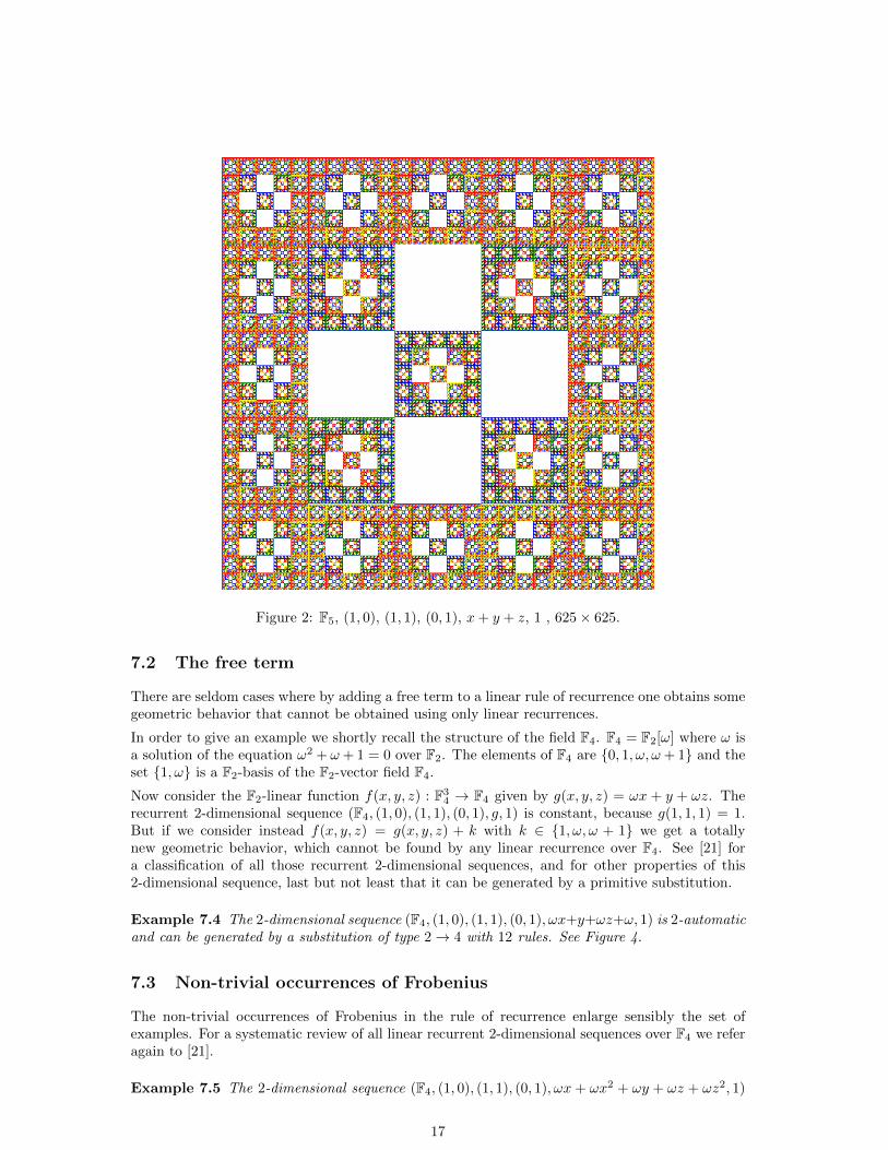
Figure 2: F5, (1, 0), (1, 1), (0, 1), x+ y + z, 1 , 625× 625.

7.2 The free term

There are seldom cases where by adding a free term to a linear rule of recurrence one obtains somegeometric behavior that cannot be obtained using only linear recurrences.

In order to give an example we shortly recall the structure of the field F4. F4 = F2[ω] where ω isa solution of the equation ω2 + ω + 1 = 0 over F2. The elements of F4 are {0, 1, ω, ω + 1} and theset {1, ω} is a F2-basis of the F2-vector field F4.

Now consider the F2-linear function f(x, y, z) : F34 → F4 given by g(x, y, z) = ωx + y + ωz. The

recurrent 2-dimensional sequence (F4, (1, 0), (1, 1), (0, 1), g, 1) is constant, because g(1, 1, 1) = 1.But if we consider instead f(x, y, z) = g(x, y, z) + k with k ∈ {1, ω, ω + 1} we get a totallynew geometric behavior, which cannot be found by any linear recurrence over F4. See [21] fora classification of all those recurrent 2-dimensional sequences, and for other properties of this2-dimensional sequence, last but not least that it can be generated by a primitive substitution.

Example 7.4 The 2-dimensional sequence (F4, (1, 0), (1, 1), (0, 1), ωx+y+ωz+ω, 1) is 2-automaticand can be generated by a substitution of type 2→ 4 with 12 rules. See Figure 4.

7.3 Non-trivial occurrences of Frobenius

The non-trivial occurrences of Frobenius in the rule of recurrence enlarge sensibly the set ofexamples. For a systematic review of all linear recurrent 2-dimensional sequences over F4 we referagain to [21].

Example 7.5 The 2-dimensional sequence (F4, (1, 0), (1, 1), (0, 1), ωx + ωx2 + ωy + ωz + ωz2, 1)

17

Figure 3: F5, (1, 0), (1, 1), (0, 1), 3x+ 4y + 3z + 3, 1 , 625× 625.

is 2-automatic and can be generated by a substitution of type 2→ 4 with 41 rules. See Figure 5.

7.4 Non-constant borders

The first examples of non-constant borders studied by the author were periodic borders, see[20]. It is known that all ultimately periodic sequences are k-automatic, for all k ≥ 2. Here,we prefer to present two examples with nonperiodic automatic borders. The first example usesthe Prouhet-Thue-Morse sequence, which is a morphic sequence; the second one uses the Rudin-Shapiro sequence, which can be generated by a one-dimensional substitution of type 2→ 4.

Definition 7.6 The Prouhet-Thue-Morse Sequence t(n) is a 2-automatic sequence t(n) producedby the following uniform morphism (substitution of type 1 → 2): 0 → 01, 1 → 10 with startsymbol 0. The Thue-Morse-Pascal 2-dimensional Sequence is the recurrent 2-dimensional sequence(F2, (1, 0), (0, 1), x+ y, t, t).

Example 7.7 The Thue-Morse-Pascal 2-dimensional sequence is 2-automatic and can be gener-ated by a substitution of type 4→ 8 with 15 rules. See Figure 6.

The system of substitutions ({0, 1},D, E , D1,Σ) consists of the following sets. The set D ={D1, . . . , D15} consists of the matrices:

D1 =

0 1 1 01 0 1 11 1 0 10 1 1 0

D2 =

1 0 0 10 0 0 11 1 1 01 0 1 1

D3 =

1 0 0 10 0 0 10 0 0 11 1 1 0

D4 =

0 1 1 01 0 1 10 0 1 00 0 1 1

18

Figure 4: F4, (1, 0), (1, 1), (0, 1), ωx+ y + ωz + ω, 1, 512× 512.

D5 =

1 0 1 10 0 1 00 0 1 11 1 0 1

D6 =

0 0 1 00 0 1 11 1 0 10 1 1 0

D7 =

1 0 1 10 0 1 01 1 0 01 0 0 0

D8 =

1 1 0 11 0 0 11 1 1 01 0 1 1

D9 =

0 1 0 01 0 0 01 1 1 10 1 0 1

D10 =

0 1 0 01 0 0 00 0 0 00 0 0 0

D11 =

0 0 0 00 0 0 00 0 0 00 0 0 0

D12 =

1 1 1 11 0 1 01 1 0 01 0 0 0

D13 =

0 0 1 00 0 1 10 0 1 00 0 1 1

D14 =

1 1 1 11 0 1 00 0 1 11 1 0 1

D15 =

0 0 0 00 0 0 01 1 1 10 1 0 1

The set E = {E1, . . . , E15} consists of the matrices:

E1 =

(D1 D2

D5 D6

)E2 =

(D3 D4

D7 D8

)E3 =

(D3 D4

D9 D6

)E4 =

(D1 D2

D10 D8

)

E5 =

(D3 D7

D9 D14

)E6 =

(D11 D8

D14 D6

)E7 =

(D3 D7

D7 D11

)E8 =

(D12 D13

D12 D8

)

19

Figure 5: F4, (1, 0), (1, 1), (0, 1), ωx+ ωx2 + ωy + ωz + ωz2, 1, 512× 512.

E9 =

(D1 D10

D5 D14

)E10 =

(D1 D10

D10 D11

)E11 =

(D11 D11

D11 D11

)E12 =

(D12 D12

D12 D11

)

E13 =

(D11 D8

D11 D8

)E14 =

(D12 D12

D15 D14

)E15 =

(D11 D11

D14 D14

)The matrix D1 is the start symbol, and ∀ i Σ(Di) = Ei.

We can verify by hand the first condition of Theorem 3.13. Only the substitution rules for D1,D2, D3 and D4 touch the horizontal border. Let Mi = Di ∩ (y = 0). The relevant parts ofthe substitution rules read M1 → M1M2, M2 → M3M4, M3 → M3M4 and M4 → M1M2,where M1 = M4 = 0110 and M2 = M3 = 1001. So the horizontal border is the sequence givenby start word 0110 and by the rules α : 0110 → 01101001 and β : 1001 → 10010110. Leth : {0, 1}∗ → {0, 1}∗ be the homomorphism of monoids h whose fixed point is the Prouhet-Thue-Morse sequence. The homomorphism h is defined by h(0) = 01 and h(1) = 10. The startword 0110 = h2(0) and every further complete substitution step using both rules α and β hasthe same effect as applying h2. It follows by induction that the horizontal border is exactly theProuhet-Thue-Morse sequence. The proof is similar for the vertical border.

The second condition of Theorem 3.13 has been checked using a computer program. The programgenerated a 8000× 8000 initial square of the recurrent 2-dimensional sequence, checked that thissquare was identical with the corresponding square produced by substitution, and checked thefact that all 8× 8-squares occurring in 4-position have already occurred in some 4-positions in the4000× 4000 left-upper quarter of this initial square. This way the conditions of Theorem 3.13 arefulfilled. 2

20

Figure 6: F2, (0, 1), (1, 0), x+ y, Thue-Morse, 512× 512.

For the next example we use the Rudin-Shapiro sequence, which is originally a sequence in thealphabet {+1,−1}. Because −1 does not make sense in F2 we use here an isomorphic sequenceover the alphabet {0, 1}.

Definition 7.8 The Rudin-Shapiro Sequence r(n) is a 2-automatic sequence produced by thefollowing substitution of type 2 → 4: 00 → 0001, 01 → 0010, 10 → 1101, 11 → 1110 withstart word 00. The Rudin-Shapiro-Pascal 2-dimensional Sequence is the recurrent 2-dimensionalsequence (F2, (1, 0), (0, 1), x+ y, r, r).

Example 7.9 The Rudin-Shapiro-Pascal 2-dimensional sequence is 2-automatic and can be gen-erated by a substitution of type 4→ 8 with 44 rules. See Figure 7.

7.5 Excessive recurrence

Extremely interesting are the examples of recurrence with positive excess, where the alphabet issome finite abelian p-group and the recurrence is a homomorphism of p-groups. Although theyare not proven to be automatic by Theorem 5.2, in all examples computed by the author onecan guess a substitution and then prove the identity of the 2-dimensional sequence obtained bysubstitution with the 2-dimensional sequence got by recurrence, using Theorem 3.13. We showtwo examples:

Example 7.10 The 2-dimensional sequence defined by a recurrence with system of predecessors(0, 1), (1,−1) and the rule x+ y over the field F2, with initial condition a(i, 0) = 1, a(0, j) = 1, is2-automatic and can be generated by a substitution of type 4→ 8 with 16 rules. See Figure 8.

21

Figure 7: F2, (0, 1), (1, 0), x+ y, Rudin-Shapiro, 512× 512.

Example 7.11 The 2-dimensional sequence defined by a recurrence with system of predecessors(1, 0), (1,−2), (0, 1) and the rule x + y + z over the field F2, with initial condition a(i, 0) = t(i),a(0, j) = t(j), where t is the Thue-Morse sequence starting with 0, is 2-automatic and can begenerated by a substitution of type 4→ 8 with 32 rules. See Figure 9.

Open problems:

1. Prove that every non-periodic and non-diagonal patchwork carpet has the geometric behaviorof some tensor power carpet.

2. Find a connection between the coefficients of a patchwork carpet and its geometric behavior.

3. Does Theorem 5.2 hold true for excessive recurrence?

4. Does Theorem 5.2 remain true for arbitrary homomorphisms of groups f : Gm → G, whereG is any finite abelian p-group?

5. Does Theorem 5.2 remain true in the most general setting in which we dare to formulatethat question: general recurrence and homomorphisms of finite abelian p-groups?

Up to now all examples computed by the author confirm positive conjectures for the questions 1,3, 4 and 5.

8 Appendix: The anatomy of Stairway

The recurrent two-dimensional sequence Stairway (see Figure 10) has the system of predeces-sors {(1, 0), (1, 1), (0, 1)}, constant borders a(i, 0) = a(0, j) = 1 and is given by the polynomial

22

Figure 8: F2, (0, 1), (1,−1), x+ y, 1, 512× 512.

f(x, y, z) = 2x3y3z3 + 2xy2 + 2y2z+ y over F5. The goal of this Appendix is a short study of thisrecurrent 2-dimensional sequence, in order to complete the proof of Theorem 6.1.

The function f(x, y, z) has the property f(x, y, z) = f(z, y, x). This implies that the recurrent2-dimensional sequence fulfills a(m,n) = a(n,m), i.e. is diagonally symmetric.

In spite of the fact that there are 125 triples (a, b, c) ∈ F35, we will see that only 32 triples consisting

of coordinates different from 0 really appear in the sequence. In order to understand how thesequence works, it is useful to enumerate them here. All rules of recurrence will be represented inthe form:

R =

(y zx f(x, y, z)

)Because of the diagonal symmetry stated above, if a rule R does concretely occur in the recurrent2-dimensional sequence, its transposed RT also occurs in the sequence. This fact help us for afaster and easier enumeration of the rules.

We change the notation of the elements of F5 \ {0} in the following way: 1 = a, 2 = B, 3 = Aand 4 = b. In Figure 10 you see 1 = red, 2 = green, 3 = blue and 4 = yellow. According to thisnotation, there are:

6 Sporadic Rules

S1 =

(a aa B

), S2 =

(a aB A

), ST

2 , S3 =

(B AA b

), S4 =

(A Ab a

), ST

4 .

2 Square Start Rules

N1 =

(a AA a

), N2 =

(b BB b

).

23

Figure 9: F2, (1, 0), (1,−2), (0, 1), x+ y + z, Thue-Morse, 512× 512.

4 Alternate Square Margin Rules

M1 =

(A Ba b

), MT

1 , M2 =

(B Ab a

), MT

2 .

4 Exterior Stripe Rules

E1 =

(A AB B

), ET

1 , E2 =

(B BA A

), ET

2 .

4 Interior Stripe Rules

I1 =

(a ab b

), IT1 , I2 =

(b ba a

), IT2 .

2 Wave Rules

W1 =

(A AA B

), W2 =

(B BB A

).

4 Square Corner Rules

C1 =

(A Aa A

), CT

1 , C2 =

(B Bb B

), CT

2 .

2 Diagonal Rules

D1 =

(a bb b

), D2 =

(b aa a

).

24

Figure 10: F5, (0, 1), (1, 1), (1, 0), 2x3y3z3 + 2xy2 + 2y2z + y, 1, 58× 58.

4 Monochrome Square Margin Rules

Q1 =

(a aA A

), QT

1 , Q2 =

(b bB B

), QT

2 .

This enumeration of matrices must not be confounded with seemingly similar lists written downin Section 7. All those sets of matrices are left-hand sides of substitution rules, so they will finallybuild together the set Dd(a) for some 2-dimensional sequences a. In other words, those d × dmatrices will arise in the respective 2-dimensional sequences in d-positions. On the other side, therules of recurrence listed here build the covering C2(a) for the 2-dimensional sequence a calledStairway.

Definition 8.1 Let t(n) = n(n + 1)/2 be the n-th triangular number. Let Tn be the squarestarting at (t(n) + 1, t(n) + 1) of edge-length n+ 1, that is T (n) = {t(n) + 1, . . . , t(n) + n+ 1} ×{t(n) + 1, . . . , t(n) + n + 1}. The eck-points of T (n) are: e(n) = (t(n) + 1, t(n) + 1), v(n) =(t(n) + n + 1, t(n) + 1), f(n) = (t(n) + n + 1, t(n) + n + 1) and w(n) = (t(n) + 1, t(n) + n + 1).The square T (n) contains its eck-points.

Definition 8.2 The wave V (n) consists of the union of the sets {v(n) + (1,−1) + (k, k) | 0 ≤ k ≤n+ 1} and its mirrored image along the diagonal {w(n) + (−1, 1) + (k, k) | 0 ≤ k ≤ n+ 1}. Everysegment is parallel to the diagonal and consists of n + 2 elements. Let i(n) = v(n) + (1,−1)and j(n) = w(n) + (−1, 1) be the two initial points of V (n). Let x(n) = v(n) + (n + 2, n) andy(n) = w(n) + (n, n+ 2) be the two final points of V (n).

Definition 8.3 A stripe is a vertical or horizontal finite or infinite subword of the 2-dimensionalsequence Stairway, consisting of at least two equal letters.

25

Lemma 8.4 Only the elements 1, 2, 3, 4 ∈ F5 (that have been renamed as a, B, A, b) really occurin Stairway and only the given 32 rules of recurrence are needed to constuct it. The SporadicRules S are applied only once respectively, all other rules occur infinitely often. Every triangle(e(n) − (0, 1))i(n − 1)x(n − 1) consists of n + 1 alternating vertical stripes in A and B. Everysegment of the wave V (n) consists of alternating letters A and B. The first letter of a segment ofV (n) is always the same as the last letter of a segment of V (n−1). The squares T (n) in Stairwayconsist only of the letters a and b. The letter occurring in e(n) is always the same as the letteroccurring in f(n− 1). The diagonal of Stairway starts with a, B, b, a and continues as follows:

a |B | b, a | a, b, a | a, b, a, b | b, a, b, a, b | b, a, b, a, b, a | a, . . .

Proof: The proof works by induction over the sets M(i), where M(1) = {0, 1, 2, 3} × N ∪ N ×{0, 1, 2, 3} and for n ≥ 2, M(n) = {t(n) + 1, . . . , t(n) + n + 1} × {x ∈ N |x ≥ t(n) + 1} ∪{x ∈ N |x ≥ t(n) + 1} × {t(n) + 1, . . . , t(n) + n + 1}. This is possible because the system ofpredecessors {(0, 1), (1, 1), (1, 0)} has excess = 0 and makes possible both a row-wise and a column-wise recurrence.

Induction start. By constructing M(1) we apply every Sporadic Rule once and the Rule D2 once.The result is the square T (1) of the form: (

b aa a

).

On the left border (respectively under the bottom border) of the square T (1) we apply Q1 (re-spectively QT

1 ). We get that T (1) is bordered by A’s. At a(4, 1) and a(1, 4) we apply W1, ata(5, 2) and a(2, 5) we apply W2, at a(6, 3) and a(3, 6) we apply again W1 - and so we producedthe wave V (1). Both branches of V (1) have colors A, B, A respectively. Left and downwards fromV (1) there are only monochrome stripes in colors A, B, A, parallel to the axes, so the trianglee(2) − (0, 1), i(1), x(1) consists of 3 alternating vertical stripes in A and B. The segments of thewave V (1) bend an A-stripe and a B-stripe with 90◦. Finally we observe that the points i(2)and j(2) are also colored in M(1) by the rule E1 and respectively ET

1 , an that they are neigh-bors with x(1) and respectively y(1) on the same line (column) so they all get the same color:a(x(1)) = a(i(2)) = a(y(1)) = a(j(2)). The diagonal sequence constructed so far is a,B, b, a.

Induction Step. Suppose that we have already constructed the set M(n− 1) and we are about toconstruct M(n). The first point of M(n) is e(n), which is constructed using an appropriate SquareStart Rule and consequently has the same color as f(n− 1). Remember that M(n− 1) containedthe triangle e(n)− (0, 1), i(n− 1), x(n− 1), consisting of n+ 1 vertical stripes in A and B. Frome(n) we continue horizontally with the rules M1 and M2, since we arrive at v(n) (we continuevertically with the rules MT

1 , MT2 since we arrive at w(n)). Here one has got the configurations:(

a(x(n− 1)) = C a(i(n)) = Cv(n) C

),

(a(y(n− 1)) = C a(w(n)) = C

j(n) C

).

The points x(n − 1), i(n), y(n − 1), j(n) have already been constructed in M(n − 1) accordingto the hypothesis of induction and have all the same color C ∈ {A,B}. By the rules Ci the newpoint to be constructed is in both cases a C. The construction of the square T (n) is closed now by

applying the rules Q(T )i for the last two edges, and the rules I

(T )i , Di inside T (n). We check that

all the letters used for T (n) are a and b, and that the edge-length of T (n) equals the length of onesegment of the wave V (n−1), which is (n−1)+2 = n+1. Finally, in the rest of M(n) we apply theExterior Stripe Rules, then the Wave Rules, and finally again the Exterior Strip Rules. By the firstapplication of the Exterior Stripe Rules we get the triangle e(n+ 1)− (0, 1), i(n), x(n) consistingof n + 2 many alternating stripes in A and B, and its mirrored image along the diagonal. Thenwe construct the wave V (n), and the infinite stripes starting by the wave segments. In particularwe observe that a(i(n+ 1)) = a(x(n)) = a(j(n+ 1)) = a(y(n)) because the points i(n+ 1) is the

26

right neighbor of x(n) on a horizontal stripe (because j(n+ 1) is the downward neighbor of y(n)in a vertical stripe). At the diagonal sequence constructed so far we append an alternated wordof length n + 1 in a and b which starts with the same letter in which the last appended word oflength n has ended. 2

Acknowledgements: The author thanks both anonymous referees for independently suggestinga shorter proof of the fact that images of polynomials are not automatic, and for their great effortto improve the whole paper.

References

[1] J.-P. Allouche, J. Shallit: Automatic sequences - theory, applications, generalizations.Cambridge University Press, 2003.

[2] J.-P. Allouche, J. Shallit: The ubiquitous Prouhet-Thue-Morse sequence. Sequences andtheir applications (Singapore 1998), Springer Series Discrete Mathematics in TheoreticalComputer Science, Springer, London, 1 - 16, 1999.

[3] J.-P. Allouche, F. von Haeseler, H.-O. Peitgen, A. Petersen, G. Skordev: Auto-maticity of double sequences generated by one-dimensional linear cellular automata. Theo-retical Computer Science, 188, 195 - 209, 1997.

[4] P. Arnoux, V. Berthe, T. Fernique, D. Jamet: Functional stepped surfaces, flips andgeneralized substitutions. Theoretical Computer Science 380, 251 - 265, 2007.

[5] M. Baake, R. V. Moody (editors): Directions in Mathematical Quasicrystals. CRMMonograph Series, AMS, Providence, RI, 2000.

[6] A. Cobham: Uniform tag sequences. Mathematical Systems Theory, 6, 164 - 192, 1972.

[7] D. Frettloh: Duality of model sets generated by substitution. Revue Roumaine deMathematiques Pures et Appliquees, 50, 619 - 639, 2005.

[8] B. Grunbaum, G.C. Shephard: Tilings and Patterns. Dover Publications, 2012.

[9] J. Kari: Theory of cellular automata: a survey. Theoretical Computer Science 334, 3 - 33,2005.

[10] B. B. Mandelbrot: The Fractal Geometry of Nature. W. H. Freeman and Company, SanFrancisco, 1982.

[11] R. V. Moody (editor): The Mathematics of Aperiodic Order. Proceedings of the NATOAdvanced Study Institute on Long Range Aperiodic Order. Kluwer Academic Publishings,1997.

[12] An. A. Muchnik, Yu. L. Pritykin and A. L. Semenov: Sequences close to periodic.Russian Mathematical Surveys, 64, 5, 805 - 871, 2009.

[13] D. E. Passoja, A. Lakhtakia: Carpets and rugs: an exercise in numbers. Leonardo, 25,1, 69 - 71, 1992.

[14] H.-O. Peitgen, P. H. Richter: The Beauty of Fractals, Images of Complex DynamicalSystems. Springer, 1986.

[15] R. Penrose: Pentaplexity: a class of of nonperiodic tilings of plane. Mathematical Intelli-gencer 2 (1), 32 - 37, 1979.

27

[16] N. Priebe Frank: Multi-dimensional constant-length substitution sequences. Topology andApplications, 152, 44 - 69, 2005.

[17] M. Prunescu: An undecidable properties of recurrent double sequences. Notre Dame Jour-nal of Formal Logic, 49, 2, 143 - 151, 2008.

[18] M. Prunescu: Self-similar carpets over finite fields. European Journal of Combinatorics,30, 4, 866 - 878, 2009.

[19] M. Prunescu: Recurrent double sequences that can be generated by context-free substitu-tions. Fractals, 18, 1, 65 - 73, 2010.

[20] M. Prunescu: Recurrent two-dimensional sequences generated by homomorphisms of finiteabelian p-groups with periodic initial conditions. Fractals, 19, 4, 431 - 442, 2011.

[21] M. Prunescu: Linear recurrent double sequences with constant border in M2(F2) are clas-sified according to their geometric content. Symmetry, 3, 3, 402 - 442, 2011.

[22] M. Prunescu: The Thue-Morse-Pascal double sequence and similar structures. ComptesRendus - Mathematique 349, 939-942, 2011.

[23] P. Prusinkiewicz, A. Lindenmayer: The Algorithmic Beauty of Plants. Springer Verlag,1996.

[24] R. M. Robinson: Undecidability and nonperiodicity for tilings of the plane. InventionesMathematicae, 12(3), 177 - 209, 1971.

[25] G. Rozenberg, A. Salomaa (editors): Lindenmayer Systems: Impacts on TheoreticalComputer Science, Computer Graphics, and Developmental Biology. Springer Verlag, 1992.

[26] O. Salon: Suites automatiques a multi-indices. Seminaire de Theorie des Nombres de Bor-deaux, Expose 4, (1986 - 1987), 4-01-4-27; followed by an Appendix by J. Shallit, 4-29A-4-36A.

[27] O. Salon: Suites automatiques a multi-indices et algebricite. Comptes Rendus de l’Academiedes Sciences de Paris, Serie I, 305, 501 - 504, 1987.

[28] J. E. Socolar, J. M. Taylor: An aperiodic hexagonal tile. Journal of CombinatorialTheory, Series A 118, 2207-2231, 2011.

[29] J. M. Taylor: Aperiodicity of a functional monotile. http://www.math.uni-bielefeld.de/sfb701/files/preprints/sfb10015.pdf

[30] H. Wang: Proving theorems by pattern recognition II. Bell System Techical Journal 40(1):1- 41, 1961.

[31] S. J. Willson: Cellular automata can generate fractals. Discrete Applied Mathematics, 8,91 - 99, 1984.

[32] S. Wolfram: A New Kind of Science. Wolfram Media, ISBN 1-57955-008-8, 2002.

28