147

F-x linear prediction filtering of seismic images

Mark P. Harrison

ABSTRACT

The f-x linear prediction filtering algorithm is reviewed and tested on severalsynthetic images. It is found that the f-x filter, when applied to noise-free synthetics,produces little or no attenuation of continuous layers, but does laterally smear sharpdiscontinuities. On noisy synthetic images, numerical measurements indicate that the f-xfilter performs better at attenuating random noise than does the f-k filter. The f-x filter,however, produces greater lateral smearing of discontinuities than does the f-k filter. Theresidual noise after f-x filtering still appears fairly random, and the filter does not give riseto the same type of coherent "streaks" that a severe f-k filter is seen to create. In addition,the f-x filter is able to extract the signal without any guidance from the user, whereas an f-kdip reject filter must be manually selected, usually after inspection of a f-k spectrum plot.The f-x filter, however, is not able to discriminate between coherent noise with large dipand true events. Application of the f-x filter to an actual seismic image produces goodresults, and no attenuation of coherent signal is seen to occur.

INTRODUCTION

The signal-to-noise ratio for converted-wave stack images is often poor. Thisusually necessitates the application of some sort of image noise attenuation process, oftenin the form of f-k (frequency-wavenumber) or Karhunen-Loeve filtering (Jones and Levy,1987). This paper looks at a different approach to signal-enhancement, f-x filtering, inwhich the seismic image is modelled as being composed of a number of linearly-coherentreflections. This justifies the use of a prediction method in the spatial direction of the f-xdomain to optimally extract linear features and suppress random noise. This method wasfirst proposed for seismic data by Canales (1984), and has since been elaborated upon byothers (e.g. Gulunay, 1986). In the following sections the theory behind the method willbe reviewed and a comparison of the relative performance of f-x and f-k filtering will bemade.

THEORY

A seismic image represents a collection of zero-mean amplitude values that arefunctions of time t and horizontal location x (trace number). The image can usually bemodelled at some scale (Canales, 1984) as being composed of a number N of continuousdipping reflectors, each with slope si, i.e.,

N

a (t,x)= _ wi * _(t-ti)i:l , (1)

148

where w I is the temporal wavelet associated with the i'th reflector, convolved with a Diracspike located at time ti, and

ti = '_i + six.

Xl is the intercept time at some reference x-location, and sl is the slope of the reflector.Taking the fourier transform of equation 1 w.r.t time gives

N

a(co,x) = _ Wi((o) e-J°(_'_)i=l

where Wl(a)) is the fourier transform of the wavelet wl(t). This can be rewritten as

N

a(c0,x) = _ Ci(co)e-J_xi=l

where Cl(o)) is a complex function of co only. This shows that each frequency, whenviewed in the x-direction, is just a sum of weighed sinusoids of varying amplitudes andperiods, implying that changes in a frequency component in the x-direction are predictable.

Given this predictable nature, it is possible to design a unit-distance predictionoperator for each frequency that gives, in the least-squares sense, the most likely value forthe next sample based on previous samples. This leads to the design of a complex least-squared-error prediction filter. The theory behind complex prediction filtering can be foundin Treitel (1974), and is reviewed here. Letting the vector f be the prediction operator oflength m+l and the vector _ be the predicted values of a, then, for each frequency, the filterequations can be written as

a00 ... 0al a0• al

• = 0 an ao-, 0

_am+n/

an.1

or

_= Af,

where the ai are samples in the x-direction and the co subscript has been dropped. Definingthe desired output as the vector d, which, in this case, is just the sequence advanced by onesample, then the prediction error e will be

e=d-_

=d- Af,and the error energy will be

I = erie

where eII is the transposed complex conjugate ofe. The error energy becomes

149

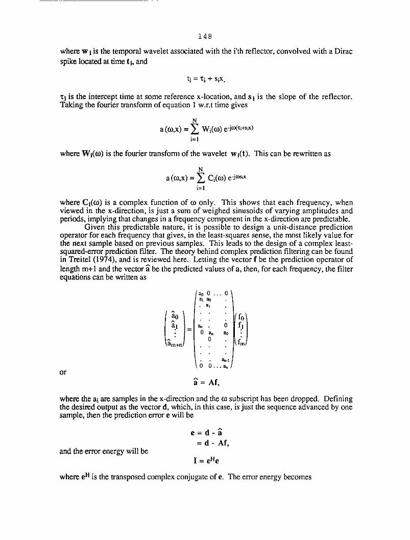
I = (d-Af)H(d-Af)= dHd. ftfArl d _ dHAf + fHAHAf.

The error energy can be minimized by taking the derivative w.r.t, the filter vector f andsetting to zero, i.e.,

_)f- dHA+fHAHA=0,or

fHAHA = dHA. (2)

Takingthecomplexconjugateandtransposing,thisbecomes

AHAf = AHd.

Def'ming the complex autocorrelation matrix R as

R = AHA

and the complex cross-correlation matrix g as

g=And,then equation 2 becomes

Rf = g. (3)

These are the complex-valued normal equations that must be solved for the complex filter f.The complex matrix R can be written in the form

R=P+jQ

where P is real and symmetric, and Q is real and skew-symmetric, i.e.,

Q_ = -Q

where Qt is the transpose of Q. Treitel (1974) shows that by breaking equation 3 into it'sreal and imaginary parts, it can be rewritten as a second matrix equation;

[g"l (4)

where Re and Im designate the real and imaginary parts of a function. This real-valuedmatrix equation can be solved to give the filter coefficients f. For the process being studiedhere, the g vector is just the first sub-diagonal column of the R matrix, plus one additionallag. The left matrix in equation 4 is block-Toeplitz (Treitel, 1974), and can be invertedusing a Levinson-like recursion given by Robinson (1967).

Solving Equation 4 will result in the prediction operator to be applied in the +xdirection. Prediction can also be done in the -x direction, giving left and right predictionoperators. For prediction in the -x direction, reversing the sample order and going througha similar derivation leads to the folowing;

150

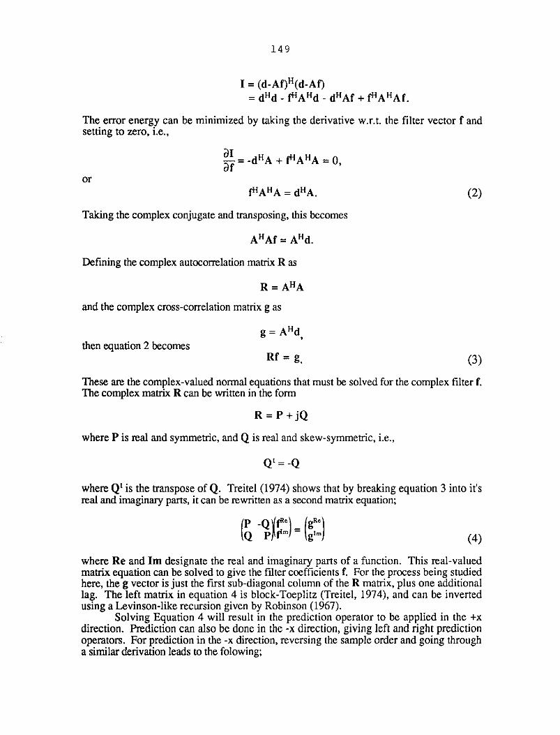
R*L = g*.

Taking the complex conjugate, this becomes

Rf.* = g,

which shows that the -x prediction operator is just the complex-conjugate of the +xprediction operator. A single filter, incorporating both +x and -x prediction, is then givenby

I" "f*mfm'l f_o_ f 1,2 ....'2'v'2 (5)

where the coefficients have been divided by 2 to give proper normalization. Thecomputation and application of this filter to the complex series a(x) for each frequency thengives the prediction-filtered set _(t.o,x), which is then inverse-transformed to give the f-xfiltered output.

A difference image can be constructed by taking the point-by-point differencebetween the input image and the filtered image;

d(t,x)=a(t,x)-_(t,x) (6)

and is often useful in evaluating the performance of the filter.

METHOD AND RESULTS

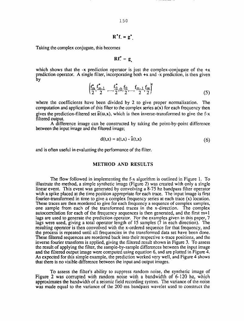
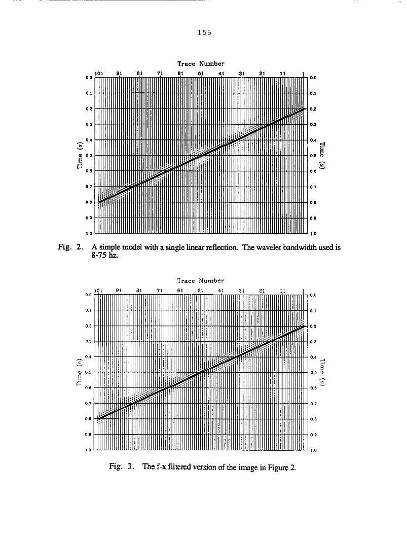
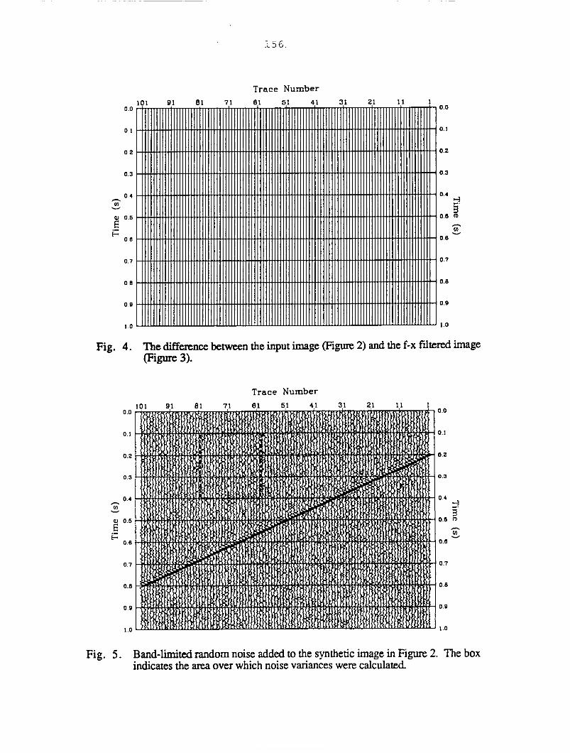
The flow followed in implementing the f-x algorithm is outlined in Figure 1. Toillustrate the method, a simple synthetic image (Figure 2) was created with only a singlelinear event. This event was generated by convolving a 8-75 hz bandpass filter operatorwith a spike placed at the time position appropriate for each trace. The input image is firstfourier-transformed in time to give a complex frequency series at each trace (x) location.These traces are then reordered to give for each frequency a sequence of complex samples,one sample from each of the transformed traces in the x-direction. The complexautocorrelation for each of the frequency sequences is then generated, and the first m+llags are used to generate the prediction operator. For the examples given in this paper, 7lags were used, giving a total operator length of 15 samples (7 in each direction). Theresulting operator is then convolved with the x-ordered sequence for that frequency, andthe process is repeated until all frequencies in the transformed data set have been done.These Falteredsequences are reordered back into their respective x-trace positions, and theinverse fourier transform is applied, giving the filtered result shown in Figure 3. To assessthe result of applying the filter, the sample-by-sample differences between the input imageand the filtered output image were computed using equation 6, and are plotted in Figure 4.As expected for this simple example, the prediction worked very well, and Figure 4 showsthat there is no visible difference between the input and output images.

To assess the filter's ability to suppress random noise, the synthetic image ofFigure 2 was corrupted with random noise with a bandwidth of 6-120 hz, whichapproximates the bandwidth of a seismic field recording system. The variance of the noisewas made equal to the variance of the 200 ms bandpass wavelet used to construct the

151

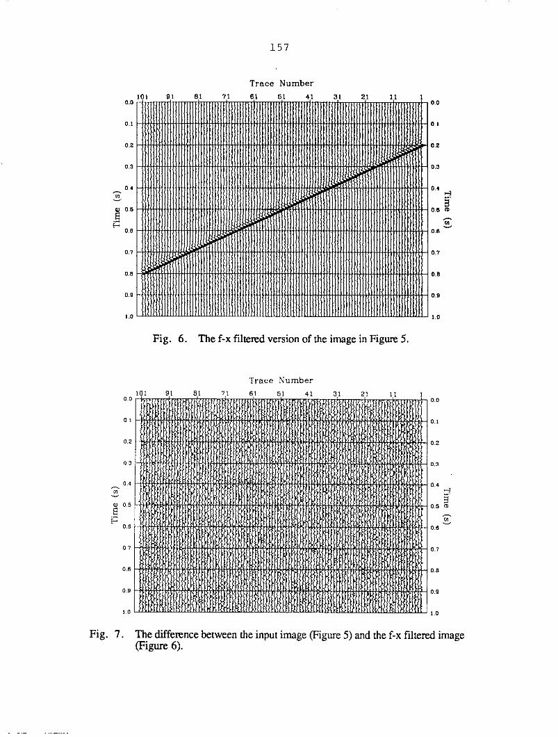
original synthetic. The resulting image is shown in Figure 5, and is seen to have a severenoise level, close to the upper limit of that normally found on a seismic image. In order toroughly assess the filter's noise-suppression capabilities, a portion of the image, outlined inFigure 5, was selected over which the noise variance levels before and after filtering werecomputed. In this case, it was found that the filter attenuated the dipping reflector by about35%. To account for this, the filtered image was scaled by a constant factor to bring theamplitudes of the dipping event closer to it's original level (Figure 6), and a differenceimage was computed (Figure 7). From the difference image, it is seen that a substantialamount of noise has been rejected. Measurements within the control portion of the imageindicate a reduction in the noise variance of 16.6 db.

An f-k filter was also applied to the noisy image for comparison, giving the resultshown in Figure 8. A comparison of the f-k filtered image and the f-x filtered image(Figure 6) shows that both have done a comparable job of attenuating the noise. The noiseleft by the f-k f'dter appears very coherent, whereas the noise left by the f-x is more randomand lower frequency. Measurements within the control portion indicate a reduction in thenoise variance of 14.8 db, compared to 16.6 db for the f-x filter.

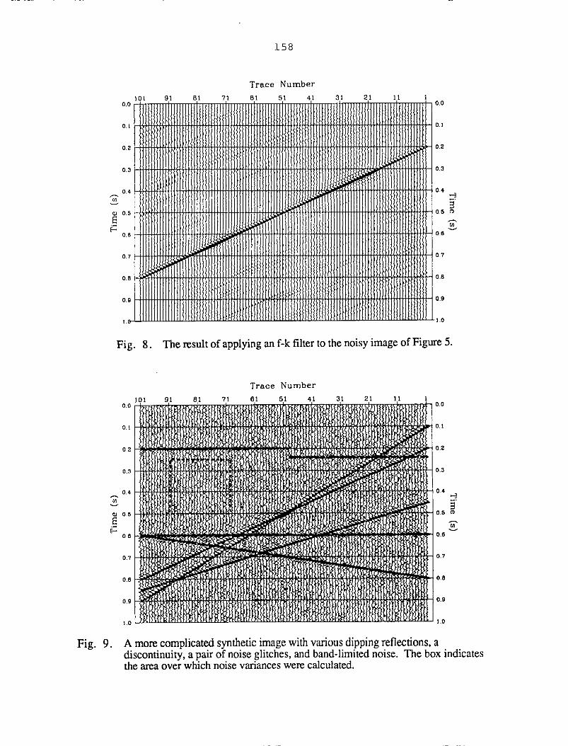
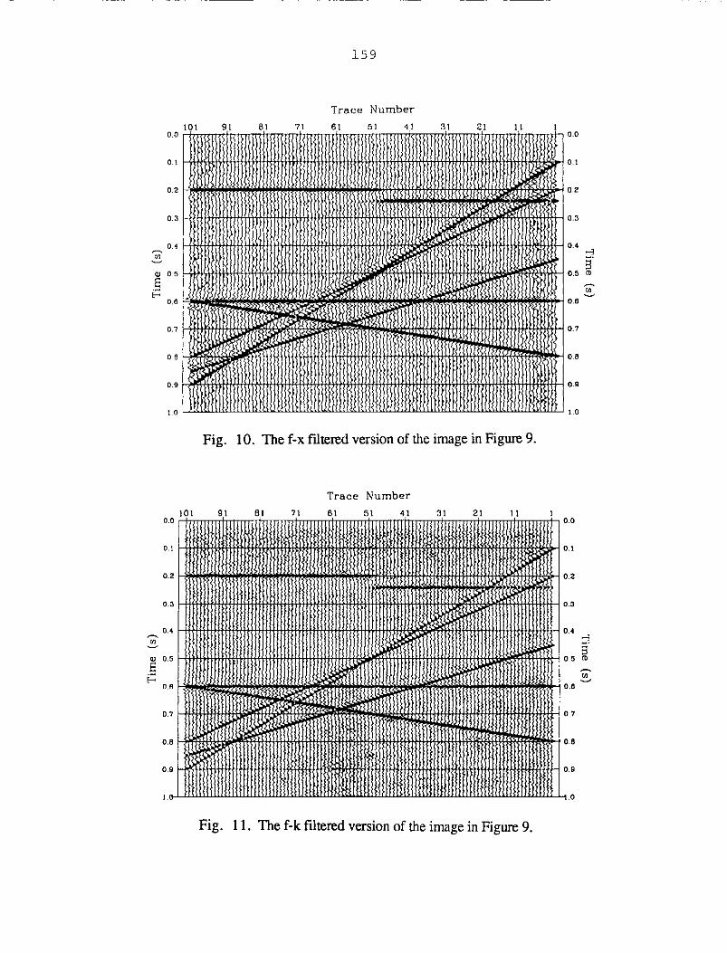
A more complicated synthetic was constructed, having reflectors withdiscontinuities and conflicting dips, as well as two large-amplitude noise glitches. Randomnoise identical in amplitude and frequency to that used in the previous example was added,giving the results shown in Figure 9. A control portion for attenuation comparison wasalso selected for this image, and is outlined in the figure. The result of f-x filtering theimage is shown in Figure 10. The two large-amplitude glitches are largely removed, andthere is little smearing of the glitches into adjacent traces. The discontinuity on the top flathorizon is seen to have been spread horizontally over a distance of seven traces (the widthof the prediction filter). The difference image, which is not shown here, shows about a15% loss of amplitude on the two steepest events, relative to the other reflectors.Measurements made within the control portion give a reduction in noise variance of 8.4 db.

An f-k filter was also applied to the image of Figure 9, giving the result shown inFigure 11. Comparison of the f-x filtered image (Figure 10) and the f-k filtered image(Figure 11) indicates that both methods have achieved roughly the same amount of noiseattenuation, with the noise remaining in the f-k filtered image again appearing higherfrequency and less random than in the f-x filtered image. The f-k filter is seen to produceless lateral tapering of the discontinuity on the top flat event than does the f-x filter.Measurements made within the control portion indicate a 4.7 db reduction in the noisevariance, compared to 8.4 db for the f-x filter.

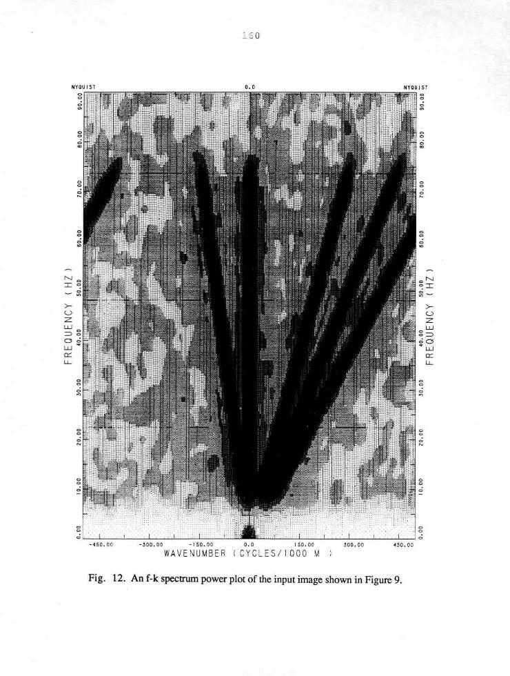
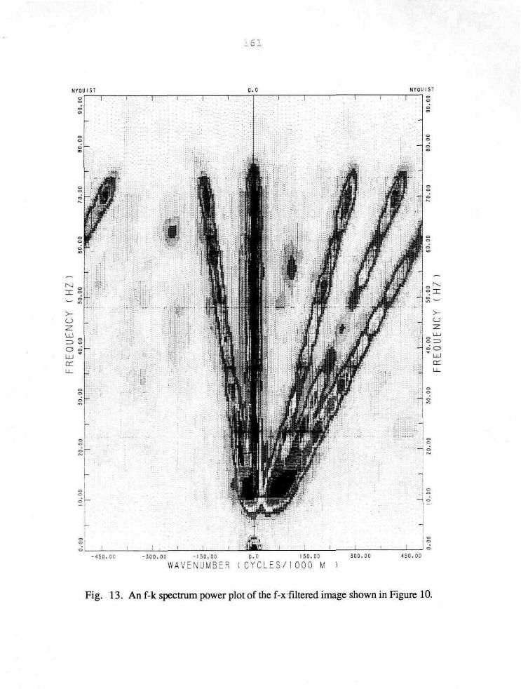
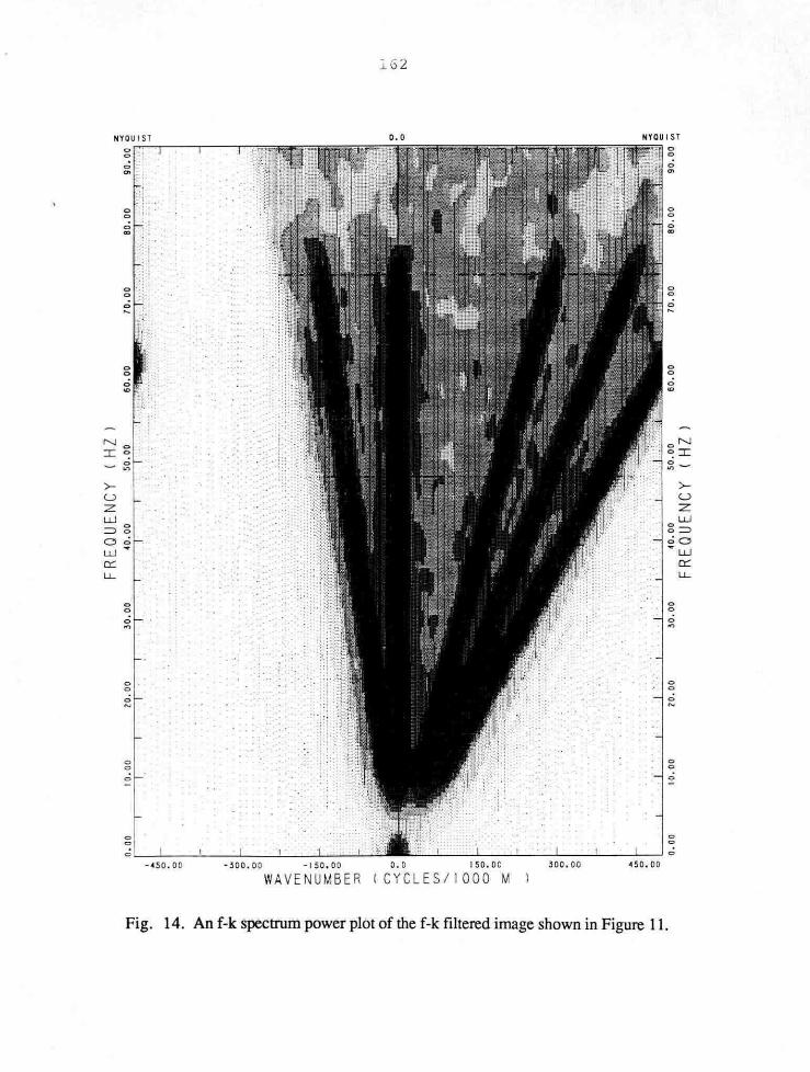
Plotted in Figure 12 is an f-k power spectrum of the noisy input image, whichshows the noise to be evenly distributed over the entire f-k spectrum. The most steeply-dipping event is seen to alias at frequencies greater than about 65 hz. An f-k power plot ofthe f-k f'fltered section of Figure 11 is displayed in Figure 14, and shows that the noise hasbeen removed from the spectrum everywhere except within the wedge enclosing thedipping events. The filter has also removed the aliased frequencies of the most steeply-dipping event, which produces a change in waveform shape for that event. Figure 13 is anf-k power plot of the f-x filtered image of Figure 10, from which it is seen that the noisehas been uniformly attenuated throughout the spectrum, including within and beneath thesignal band where f-k filtering has had no effect.

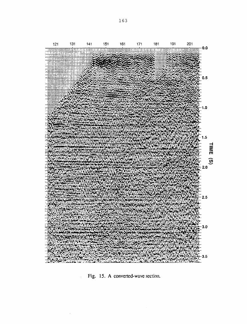
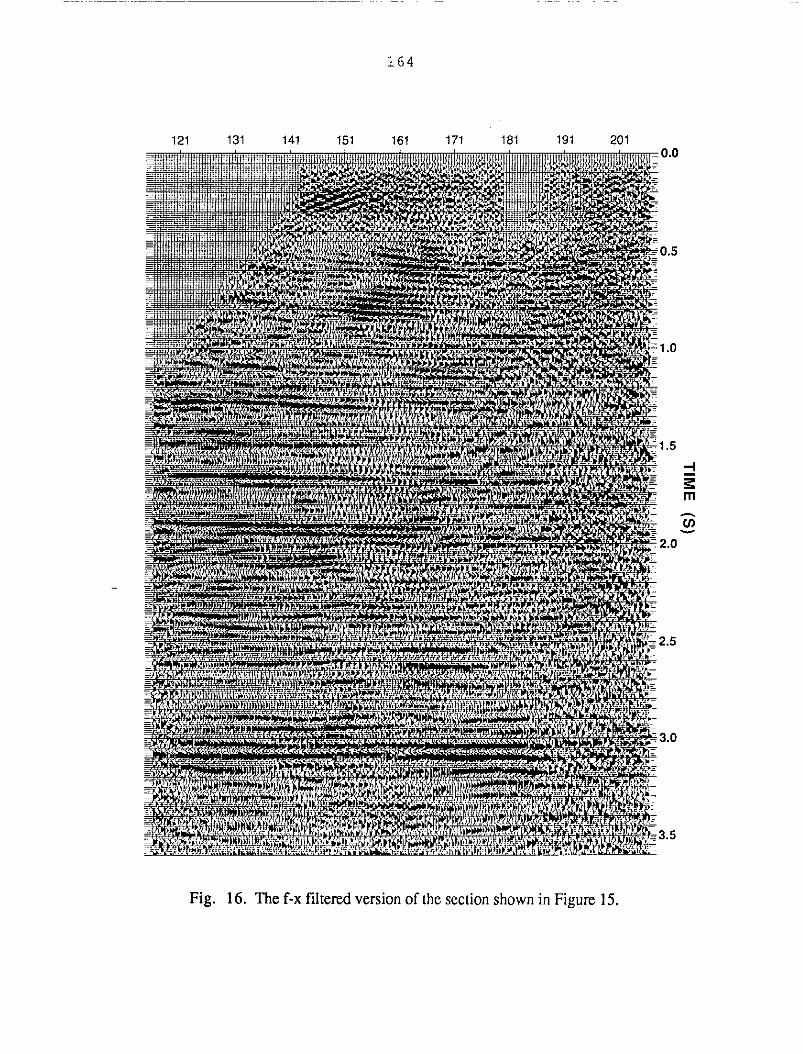
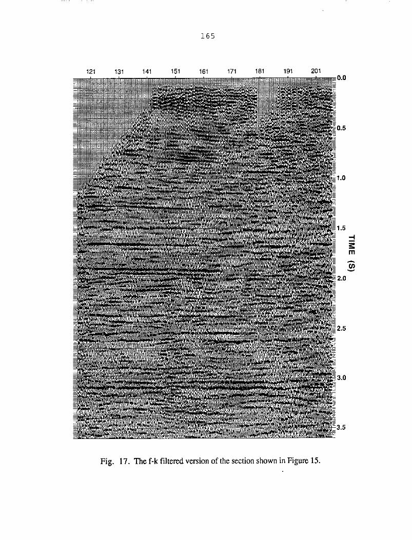
As a final example, the f-x filter was run on the radial-component section of lineFS90-1 in the Springbank, Alberta area (Lawton and Harrison, 1990) The original and f-xfiltered sections are displayed in Figures 15 and 16 respectively. For comparison, an f-kfilter was also applied, giving the section shown in Figure 17. The f-x filter is seen to give

152

better overall continuity than does the f-k filter. The very high-dip noise trains have notbeen attenuated by the f-x filter, but have been removed by the f-k filter.

DISCUSSION

The main parameters that the user of an f-x filter has to decide upon are the lengthof the prediction filter and the size of the window in which it is designed. In thecomplicated synthetic, a longer operator and/or a smaller window size probably would havegiven better preservation of the most steeply-dipping events, but no work has been done toconfirm this. The choice of seven lags for the operator length appears to work well in theexamples presented here, but it is possible that a longer operator might have producedbetter results. A major constraint on the length of the filter operator, however, is thecomputational cost of having to design a filter for each individual frequency. In order thatthe method be practical, it is desirable to keep the number of lags used as small as possible.

An area for further testing of the f-x filter is in cases where events are curved, andhave amplitude variations. If these events are altered or discarded by the filter, then themethod may have limited use in areas of large sub-surface structure. Also, Gulunay (1986)gives a proof that f-x filtering does not work correctly if events with conflicting dips arepresent, as could occur in structured areas. From the synthetic images shown here, as wellas other tests, it appears, however, that the filter still performs well when this happens.

From the synthetic examples, it is seen that the f-x filter is better at attenuatingrandom noise than is the f-k f'flter. The residual noise after f-x filtering still appears fairlyrandom, and it does not give rise to the same type of coherent "streaks" that a severe f-kfilter is known to produce. In addition, the f-x filter is able to extract the signal without anyguidance from the user, whereas an f-k dip reject filter must be manually selected, usuallyafter inspection of an f-k spectrum plot. The f-x filter therefore appears to have someimportant advantages over the f-k filtering method. It is seen from Figure 16 that the f-xfilter is not able to distinguish coherent linear noise from true reflections, which can be adisadvantage. It is possible that better results could be obtained in some cases by usingboth an f-x filter to remove random noise, and a mild f-x to remove high-dip coherentnoise.

CONCLUSIONS

The f-x linear prediction filter was reviewed and tested on several synthetic images.It was found that the filter, when applied to noise-free synthetics, produces little or noattenuation of continuous layers, but does laterally smear sharp discontinuities. On noisysynthetic images, numerical measurements indicate the f-x filter performs better atattenuating random noise than the f-k filter. The residual noise after f-x filtering stillappears fairly random, and the filter does not give rise to the same type of coherent"streaks" that a severe f-k filter was seen to produce. In addition, the f-x filter is able toextract the signal without any guidance from the user, whereas an f-k dip reject filter mustbe manually selected, usually after inspection of a f-k spectrum plot. The f-x filter is notable to attenuate coherent dipping noise, which appears to the algorithm as valid signal.Application of the f-x filter to an actual seismic image produced results which comparedfavorably to those obtained by f-k filtering.

153

REFERENCES

Canales, L.L., 1984, Random noise attenuation: Presented at the 54th Ann. Mtg., Soc. Explor. Geoph.Gulunay, N., 1986, FXDECON and complex Wiener prediction filter: Presented at the 56th Ann. Mtg.,

Soc. Explor. Geoph.Jones, I.F., and Levy, S., 1987, Signal-to-noise ratio enhancement in multi-channel seismic data via the

Karhunen-Loeve transform: Geophysical Prospecting, v. 35, 12-32.Lawton, D., and Harrison, M., 1990, A two-component reflection seismic survey, Springbank, Alberta: in

this volume.

Robinson, E.A., 1967, Multichannel time series analysis with digital computer programs: San Francisco,Holden-Day.

Treitel, S., 1974, The complex wiener f'flter: Geophysics, v. 39, 169-173.

= 51]

Input image da|a Seta(t,x)

Fourier transform in time

a(t,x)_ a(_,x)

$|

Reorder by frequency [

Ia(x) foreach co

Generate the autocorrelationfunctionand prediction filter for each frequency

IFilter the offset sequences

a(x) _(x) foreach co

Reorder by offset

Inverse fouriertransform

_(_,x) _ a(t,x)

+Compute the difference image

d(t,x) = a(t,x) - _(t,x)

Fig. 1. Process flowchart for the fix filtering algorithm.

155

TraceNumber

101 91 81 71 61 51 41 31 21 11 0.0

I__H__i__H__H[__i__________I_]____i__i__________i_____i____HH_H_i______________ij__!i____H_iH_i__H_i_______i____i__H_____i___i____i_iii__H'___i_i____i_______H_HHH__°'°._[_H_i_i_I_H_I_L_]_j_ °'o,lllllllllll]lllIIIIIII tlll_llllllllllllllll°_

Zo.ollllll]lllillllllllllHiiiilllillliilllilltllll/_llllllJillllllllHiilllio.,io_lllllllllllllllll[llll[llllllllllll_llllllllEl[llllltil[lllilllllllllllilllillltl°'o, I111_1 IIII °°o8_llllllllllllllllllllllllllllllllHIIII]lllllllllllll]HIIIIlllllllllllllllill°"o°_l IIIIIIIIII]ll IJIJI]llllJlll]2i,ioi__i__i______i_____H___________i____iI___i______i________i______i___i____i_i__iI______I__________._°

Fig. 2. A simple model with a single linear retlection. The wavelet bandwidth used is8-75 hz.

Trace Number

101 91 81 71 61 51 41 31 21 11 1O0 O0

0.1 0.1

02 02

03 O0

0.4 04

z _• 05 O6 fD

EOg 0.8

0.7 0.7

0.8 0.8

0.9 09

l.O 1.0

Fig. 3. The f-x filtered version of thc imagc in Figure 2.

156.

Trace Number

81 71 61 51 41 31 21 11 !D.O 0.0

Ol O.l

02 0.2

0.3 0.:3

0.4 0.4

oJ 05 0.6

06 08

0.7 0.7

08 0.8

0_9 0.9

I0 |.0

Fig. 4. The difference between the input image (Figane2) and the f-x filtered image(Figure 3).

Trace Number

81 71 81 51 41 31 21 11 I0.0

OA

0.2

03

0.4

z_ 0.5

•0.6

0.7

0.8

0,9

1.0

Fig. 5. Band-limited random noise added to the synthetic image in Figure 2. The boxindicates the area over which noise variances were calculated.

157

Trace Number

101 91 81 71 61 51 41 31 21 11 10,0

Ol

0,2

0.3

0.4

05 •

0g

0.7

0.8

0.9

1.0

Fig. 6. The f-x filtered version of the image in Figure 5.

Trace NumberI01 91 81 71 61 51 41 31

O0 0.0

01 0,1

0.2 0.2

0 3 0,3

0.4 0.4

05 05 (D

06 0.6

0 7 0.7

0.@ 08

0.9 09

I0 I0

Fig. 7. The difference between the input image (Figure 5) and the f-x filtered image(Figure 6).

158

Trace Number

91 81 71 61 51 4] 31 21 Ii l

Fig. 8. The result of applying an f-k filter to the noisy image of Figure 5.

Trace Number

71 61 51 41 31 21 II I0.0 O0

0.I 0.I

02 0.2

0.3 0.3

0.4 04

z_1 05 05 _

0 B 0.6

0.7 O.7

0.15 08

0.9 0.9

1.0 1.0

Fig. 9. A more complicated synthetic image with various dipping reflections, adiscontinuity, a pair of noise glitches, and band-limited noise. The box indicatesthe area over which noise variances were calculated.

159

Trace Number1ol 9t 61 71 61 51 4z 31 zl zt 1

OO O0

01 01

0.2 02

0.3 0.3

04 0.4

0 5 0.5 f_

E

06 06

0.7 07

08 08

09 09

I0 10

Pig. 10. The f-x f'dtered version of the image in Figure 9.

Trace Number

101 91 fll 71 61 61 41 31 21 11 1

Fig. 11. The f-k f'fltered version of the image in Figure 9.

NYQUIST 0.0 NTQUIST

-300.00 -150.00 0.0 150.00

W A V E N U M B E R ( CYCLES/1 000 Ii300.00

Fig. 12. An f-k spectrum power plot of the input image shown in Figure 9.

161

o . o

3 0 0 . 0 0 4 5 0 . 0 0

W A V E N U M B E R ( C Y C L E S / 1 0 0 0

Fig. 13. An f-k spectrum power plot of the f-x filtered image shown in Figure 10.

62

Nrouisr

300.00

W A V E N U M B E R t C Y C L E S / 1 0 0 0

Fig. 14. Anf-kspectrumpowerplotof the f-k filtered image shown in Figure 11.

TIM

E(S

)o

.m

.o

.m

.o

.m

.o

.m

165

121 13"f 141 151 161 171 181 191 201

1.5

I'll

v

2.O

Fig. 17. The f-k fihered version ofthe section showninFigure 15.