Embed Size (px)
Citation preview

608 12. Linear Prediction
R(0)= σ2y . You can easily determine Rnorm by doing a maximum entropy extension to
order six, starting with the four reflection coefficients and setting γ5 = γ6 = 0.)
In generating yn make sure that the transients introduced by the filter have died out.Then, generate the corresponding N samples of the signal xn. On the same graph,plot xn together with the desired signal sn. On a separate graph (but using the samevertical scales as the previous one) plot the reference signal yn versus n.
b. For M = 4, design a Wiener filter of order-M based on the generated signal blocks{xn, yn}, n = 0,1, . . . ,N − 1, and realize it in both the direct and lattice forms.
c. Using the lattice form, filter the signals xn, yn through the designed filter and generatethe outputs xn, en. Explain why en should be an estimate of the desired signal sn. Onthe same graph, plot en and sn using the same vertical scales as in part (a).
d. Repeat parts (b) and (c) for filter orders M = 5,6,7,8. Discuss the improvement ob-tained with increasing order. What is the smallest M that would, at least theoretically,result in en = sn? Some example graphs are included below.
0 50 100 150 200−4
−3
−2
−1
0
1
2
3
4
time samples, n
Wiener filter inputs
y(n) x(n)
0 50 100 150 200−4
−3
−2
−1
0
1
2
3
4
time samples, n
Wiener filter − error output, M=6
e(n) s(n)
13Kalman Filtering
13.1 State-Space Models
The Kalman filter is based on a state/measurement model of the form:
xn+1 = Anxn +wn
yn = Cnxn + vn
(state model)
(measurement model)(13.1.1)
where xn is ap-dimensional state vector and yn, an r-dimensional vector of observations.The p×p state-transition matrix An and r×p measurement matrix Cn may depend ontime n. The signals wn,vn are assumed to be mutually-independent, zero-mean, white-noise signals with known covariance matrices Qn and Rn:
E[wnwTi ] = Qnδni
E[vnvTi ] = Rnδni
E[wnvTi ] = 0
(13.1.2)
The model is iterated starting at n = 0. The initial state vector x0 is assumed to berandom and independent of wn,vn, but with a known mean x0 = E[x0] and covariancematrix Σ0 = E[(x0 − x0)(x0 − x0)T]. We will assume, for now, that x0,wn,vn are nor-mally distributed, and therefore, their statistical description is completely determinedby their means and covariances. A non-zero cross-covariance E[wnvTi ]= Snδni mayalso be assumed. A scalar version of the model was discussed in Chap. 11.
The covariance matrices Qn,Rn have dimensions p×p and r×r, but they need nothave full rank (which would mean that some of the components of xn or yn would, inan appropriate basis, be noise-free.) For example, to allow the possibility of fewer statenoise components, the model (13.1.1) is often written in the form:
xn+1 = Anxn +Gnwn
yn = Cnxn + vn
(state model)
(measurement model)(13.1.3)
609

610 13. Kalman Filtering
where the new wn is lower-dimensional with (full-rank) covariance Qn. In this model,the covariances of the noise components will be E[(Gnwn)(Gnwn)T]= GnQnGT
n , Inaddition, external deterministic inputs may be present, for example,
xn+1 = Anxn + Bnun +Gnwn
yn = Cnxn + vn
(state model)
(measurement model)(13.1.4)
where un is the deterministic input. Such modifications do not affect much the essentialform of the Kalman filter and, therefore, we will use the simpler model (13.1.1).
The iterated solution of the state equation (13.1.1) may be obtained with the help ofthe corresponding p×p state-transition matrix Φn,k defined as follows:
Φn,k = An−1 · · ·Ak , for n > k
Φn,n = I
Φn,k = Φ−1k,n , for n < k
(13.1.5)
where I is the p×p identity matrix and the third equation is valid only if the inverseexists. In particular, we have Φn,0 = An−1 · · ·A0 for n > 0, and Φ0,0 = I. If the statematrix An is independent of n, then the above definitions imply that Φn,k = An−k. Wenote also the properties:
Φn,n−1 = An , n ≥ 1
Φn+1,k = AnΦn,k , n ≥ k
Φn,k = Φn,iΦi,k , n ≥ i ≥ k
(13.1.6)
It is easily verified that the solution of Eq. (13.1.1) is given by:
xn = Φn,0 x0 +n∑
k=1
Φn,kwk−1 , n ≥ 1 (13.1.7)
so that xn depends only on {x0,w0,w1, . . . ,wn−1}, for example,
x1 = Φ1,0 x0 +Φ1,1w0
x2 = Φ2,0 x0 +Φ2,1w0 +Φ2,2w1
x3 = Φ3,0 x0 +Φ3,1w0 +Φ3,2w1 +Φ3,3w2
...xn = Φn,0 x0 +Φn,1w0 +Φn,2w1 + · · · +Φn,nwn−1
and more generally, starting at time n = i,
xn = Φn,i xi +n∑
k=i+1
Φn,kwk−1 , n > i (13.1.8)
Let xn = E[xn] and Σn = E[(xn − xn)(xn − xn)T] be the mean and covariancematrix of the state vector xn. Then, it follows from Eqs. (13.1.2) and (13.1.7) and the
13.1. State-Space Models 611
independence of x0 and wn that,
xn = Φn,0x0
Σn = Φn,0Σ0ΦTn,0 +
n∑k=1
Φn,kQk−1ΦTn,k , n ≥ 1
(13.1.9)
It is straightforward to show from (13.1.9) or (13.1.1) that xn and Σn satisfy the recur-sions:
xn+1 = AnxnΣn+1 = AnΣnAT
n +Qn , n ≥ 1(13.1.10)
Indeed, subtracting (13.1.1) and (13.1.10) and using the independence of xn and wn,we find:
xn+1 − xn+1 = An(xn − xn)+wn
Σn+1 = E[(xn+1 − xn+1)(xn+1 − xn+1)T]= E[(An(xn − xn)+wn)(An(xn − xn)+wn)T]
= AnE[(xn − xn)(xn − xn)T]ATn + E[wnwT
n]= AnΣnATn +Qn
In a similar fashion, we can obtain the statistical properties of the observations ynfrom those of xn and vn:
yn = Cnxn
yn − yn = Cn(xn − xn)+vn
Σynyn = E[(yn − yn)(yn − yn)T]= CnΣnCTn +Rn , n ≥ 0
(13.1.11)
Example 13.1.1: Local Level Model. The local-level model discussed in Chap. 6 is already instate-space form:
xn+1 = xn +wn
yn = xn + vn
and represents a random-walk process xn observed in noise. The noise variances are de-fined as Q = σ2
w and R = σ2v . ��
Example 13.1.2: Local Trend Model. The local-trend model was discussed in Sec. 6.13. Letan, bn be the local level and local slope. The model is defined by,
an+1 = an + bn +wn
bn+1 = bn + un
yn = an + vn
with mutually uncorrelated noise components wn,un, vn. The model can be written instate-space form as follows:[
an+1
bn+1
]=[
1 10 1
][anbn
]+[wn
un
], yn = [1,0]
[anbn
]+ vn
The noise covariances are:
wn =[wn
un
], Q = E[wnwT
n]=[σ2w 0
0 σ2u
], R = σ2
v

612 13. Kalman Filtering
As we mentioned in Sec. 6.13, the steady-state version of the Kalman filter for this modelis equivalent to Holt’s exponential smoothing method. We demonstrate this later. ��
Example 13.1.3: Kinematic Models for Radar Tracking. Consider the one-dimensional motionof an object moving with constant acceleration, x(t)= a. By integrating this equation, theobject’s position x(t) and velocity x(t) are,
x(t)= x(t0)+(t − t0)x(t0)+1
2(t − t0)2 a
x(t)= x(t0)+(t − t0)a(13.1.12)
Suppose the motion is sampled at time intervals T, i.e., at the time instants tn = nT, andlet us assume that the acceleration is not necessarily constant for all t, but is constantwithin each interval T, that is, a(t)= a(tn), for tn ≤ t < tn+1. Then, applying Eq. (13.1.12)at t = tn+1 and t0 = tn, and denoting x(tn)= xn, x(tn)= xn, and a(tn)= an, we obtain,
xn+1 = xn +Txn + 1
2T2an
xn+1 = xn +Tan(13.1.13)
To describe an object that is trying to move at constant speed but is subject to randomaccelerations, we may assume that an is a zero-mean random variable with variance σ2
a. Ifthe object’s position xn is observed in noise vn, we obtain the model:
xn+1 = xn +Txn + 1
2T2an
xn+1 = xn +Tanyn = xn + vn
(13.1.14)
which may be written in state-space form:[xn+1
xn+1
]=[
1 T0 1
][xnxn
]+[T2/2T
]an
yn = [1,0][xnxn
]+ vn
(13.1.15)
with measurement noise variance R = σ2v , and state noise vector and covariance matrix:
wn =[T2/2T
]an ⇒ Q = E[wnwT
n]=[T4/4 T3/2T3/2 T2
]σ2a (13.1.16)
This model is, of course, very similar to the local-trend model of the previous example ifwe set T = 1, except now the state noise arises from a single acceleration noise an affect-ing both components of the state vector, whereas in the local-trend model, we assumedindependent noises for the local level and local slope.
We will see later that the steady-state Kalman filter for the model defined by Eqs. (13.1.15)and (13.1.16) is equivalent to an optimum version of the popular α–β radar tracking filter[868,869]. An alternative model, which leads to a somewhat different α–β tracking model[870,874], has state noise added only to the velocity component:[
xn+1
xn+1
]=[
1 T0 1
][xnxn
]+[
0wn
]
yn = [1,0][xnxn
]+ vn
(13.1.17)
13.1. State-Space Models 613
with R = σ2v and
wn =[
0wn
], Q = E[wnwT
n]=[
0 00 σ2
w
]
The models (13.1.15) and (13.1.17) are appropriate for uniformly moving objects subjectto random accelerations. In order to describe a maneuvering, accelerating, object, we maystart with the model (13.1.15) and make the acceleration an part of the state vector andassume that it deviates from a constant acceleration by an additive white noise term, i.e.,replace an by an +wn. Denoting an by xn, we obtain the model [874,875]:
xn+1 = xn +Txn + 1
2T2(xn +wn)
xn+1 = xn +T(xn +wn)
xn+1 = xn +wn
yn = xn + vn
(13.1.18)
which may be written in the matrix form:⎡⎢⎣ xn+1
xn+1
xn+1
⎤⎥⎦ =
⎡⎢⎣ 1 T T2/2
0 1 T0 0 1
⎤⎥⎦⎡⎢⎣ xnxnxn
⎤⎥⎦+
⎡⎢⎣ T2/2
T1
⎤⎥⎦wn
yn = [1,0,0]
⎡⎢⎣ xnxnxn
⎤⎥⎦+ vn
(13.1.19)
This leads to the so-called α–β–γ tracking filter. An alternative model may be derived bystarting with a linearly increasing acceleration x(t)= a(t)= a(t0)+(t − t0)a(t0), whoseintegration gives:
x(t)= x(t0)+(t − t0)u(t0)+1
2(t − t0)2a(t0)+1
6(t − t0)3a(t0)
x(t)= x(t0)+(t − t0)a(t0)+1
2(t − t0)2a(t0)
a(t)= a(t0)+(t − t0)a(t0)
(13.1.20)
Its sampled version is obtained by treating the acceleration rate an as a zero-mean white-noise term with variance σ2
a, resulting in the state model [876]:
⎡⎢⎣ xn+1
xn+1
xn+1
⎤⎥⎦ =
⎡⎢⎣ 1 T T2/2
0 1 T0 0 1
⎤⎥⎦⎡⎢⎣ xnxnxn
⎤⎥⎦+
⎡⎢⎣ T3/3T2/2T
⎤⎥⎦ an
yn = [1,0,0]
⎡⎢⎣ xnxnxn
⎤⎥⎦+ vn
(13.1.21)
Later on we will look at the Kalman filters for such kinematic models and discuss theirconnection to the α–β and α–β–γ tracking filters. ��

614 13. Kalman Filtering
13.2 Kalman Filter
The Kalman filter is a time-recursive procedure for estimating the state vector xn fromthe observations signal yn. Let Yn = {y0,y1, . . . ,yn} be the linear span of the observa-tions up to the current time instant n. The Kalman filter estimate of xn is defined asthe optimum linear combination of these observations that minimizes the mean-squareestimation error, and as we already know, it is given by the projection of xn onto theobservation subspace Yn. For the gaussian case, this projection happens to be the con-ditional mean xn/n = E[xn|Yn]. Let us define also the predicted estimate xn/n−1 basedon the observations Yn−1 = {y0,y1, . . . ,yn−1}. Again, for the gaussian case we havexn/n−1 = E[xn|Yn−1]. To cover both the gaussian and nongaussian, but linear, cases,we will use the following notation for the estimates, estimation errors, and mean-squareerror covariances:
xn/n−1 = Proj[xn|Yn−1]
en/n−1 = xn − xn/n−1
Pn/n−1 = E[en/n−1eTn/n−1]
and
xn/n = Proj[xn|Yn]
en/n = xn − xn/n
Pn/n = E[en/neTn/n]
(13.2.1)
We will first state the estimation algorithm, and then prove it. The Kalman filteringalgorithm for the model (13.1.1)–(13.1.2) is as follows:
Initialize in time by: x0/−1 = x0, P0/−1 = Σ0
At time n, xn/n−1, Pn/n−1, yn are available,
Dn = CnPn/n−1CTn +Rn innovations covariance
Gn = Pn/n−1CTnD−1
n Kalman gain for filtering
Kn = AnGn = AnPn/n−1CTnD−1
n Kalman gain for prediction
yn/n−1 = Cnxn/n−1 predicted measurement
εεεn = yn − yn/n−1 = yn −Cnxn/n−1 innovations sequence
Measurement update / correction:
xn/n = xn/n−1 +Gnεεεn filtered estimate
Pn/n = Pn/n−1 −GnDnGTn estimation error
Time update / prediction:
xn+1/n = Anxn/n = Anxn/n−1 +Knεεεn predicted estimate
Pn+1/n = AnPn/nATn +Qn prediction error
Go to time n+ 1
(13.2.2)The quantityDn represents the innovations covariance matrix, that is,Dn = E[εεεnεεεTn].
The innovations sequence {εεε0,εεε1, . . . ,εεεn}, constructed recursively by the algorithm, rep-resents the Gram-Schmidt orthogonalization of the observations {y0,y1, . . . ,yn} in thesense that the innovations form an orthogonal basis for the observation subspace Yn,that is, Yn is the linear span of either set:
Yn = {y0,y1, . . . ,yn} = {εεε0,εεε1, . . . ,εεεn}The orthogonality property of εεεn is expressed by:
13.2. Kalman Filter 615
E[εεεnεεεTi ]= Dnδni (13.2.3)
There are some alternative ways of writing the above equations. For example, theequation for Pn/n may be written in the equivalent ways:
1. Pn/n = Pn/n−1 −GnDnGTn = (I −GnCn)Pn/n−1
2. Pn/n = Pn/n−1 − Pn/n−1CTnD−1
n CnPn/n−1 = standard form
3. Pn/n = (I −GnCn)Pn/n−1(I −GnCn)T+GnRnGTn = Joseph form
4. Pn/n =[P−1n/n−1 +CT
nR−1n Cn
]−1 = information form
(13.2.4)
with Dn = CnPn/n−1CTn + Rn and Gn = Pn/n−1CT
nD−1n . Similarly, we can write the
Kalman gain Gn in its information form:
Gn = Pn/n−1CTnD−1
n = Pn/nCTnR−1
n (13.2.5)
It follows from the information forms that the filtered estimate may be re-expressed as:
xn/n = xn/n−1 +Gnεεεn = xn/n−1 + Pn/nCTnR−1
n (yn −Cnxn/n−1)
= Pn/n[P−1n/n −CT
nR−1n Cn
]xn/n−1 + Pn/nCT
nR−1n yn
= Pn/nP−1n/n−1xn/n−1 + Pn/nCT
nR−1n yn
from which we obtain the information form of the updating equation:
P−1n/n xn/n = P−1
n/n−1xn/n−1 +CTnR−1
n yn (13.2.6)
In the relations that involve R−1n , one must assume that Rn has full rank. The differ-
ence equation for the predicted estimate may be written directly in terms of the currentobservation yn and the closed-loop state matrix Fn = An −KnCn, as follows:
xn+1/n = Anxn/n−1 +Knεεεn = Anxn/n−1 +Kn(yn −Cnxn/n−1)
= (An −KnCn)xn/n−1 +Knyn
that is,
xn+1/n = (An −KnCn)xn/n−1 +Knyn (13.2.7)
A block diagram realization is depicted in Fig. 13.2.1. The error covariance updateequations,
Pn/n = Pn/n−1 − Pn/n−1CTnD−1
n CnPn/n−1
Pn+1/n = AnPn/nATn +Qn
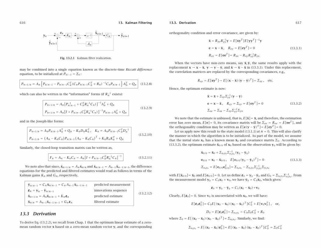
616 13. Kalman Filtering
Fig. 13.2.1 Kalman filter realization.
may be combined into a single equation known as the discrete-time Riccati differenceequation, to be initialized at P0/−1 = Σ0 :
Pn+1/n = An
[Pn/n−1 − Pn/n−1CT
n(CnPn/n−1CTn +Rn)−1CnPn/n−1
]ATn +Qn (13.2.8)
which can also be written in the “information” forms (if R−1n exists):
Pn+1/n = An[P−1n/n−1 +CT
nR−1n Cn)
]−1ATn +Qn
Pn+1/n = An[I + Pn/n−1CT
nR−1n Cn)
]−1Pn/n−1ATn +Qn
(13.2.9)
and in the Joseph-like forms:
Pn+1/n = AnPn/n−1ATn +Qn −KnDnKT
n , Kn = AnPn/n−1CTnD−1
n
Pn+1/n =(An −KnCn
)Pn/n−1
(An −KnCn
)T +KnRnKTn +Qn
(13.2.10)
Similarly, the closed-loop transition matrix can be written as,
Fn = An −KnCn = An[I + Pn/n−1CT
nR−1n Cn
]−1(13.2.11)
We note also that since, xn+1/n = An xn/n and xn/n−1 = An−1 xn−1/n−1, the differenceequations for the predicted and filtered estimates would read as follows in terms of theKalman gains Kn and Gn, respectively,
yn/n−1 = Cn xn/n−1 = CnAn−1 xn−1/n−1 predicted measurement
εεεn = yn − yn/n−1 innovations sequence
xn+1/n = Anxn/n−1 +Knεεεn predicted estimate
xn/n = An−1xn−1/n−1 +Gnεεεn filtered estimate
(13.2.12)
13.3 Derivation
To derive Eq. (13.2.2), we recall from Chap. 1 that the optimum linear estimate of a zero-mean random vector x based on a zero-mean random vector y, and the corresponding
13.3. Derivation 617
orthogonality condition and error covariance, are given by:
x = RxyR−1yyy = E[xyT]E[yyT]−1y
e = x− x , Rey = E[eyT]= 0
Ree = E[eeT]= Rxx −RxyR−1yyRyx
(13.3.1)
When the vectors have non-zero means, say x, y, the same results apply with thereplacement x → x − x, y → y − y, and x → x − x in (13.3.1). Under this replacement,the correlation matrices are replaced by the corresponding covariances, e.g.,
Rxy = E[xyT]→ E[(x− x)(y− y)T]= Σxy , etc.
Hence, the optimum estimate is now:
x = x+ ΣxyΣ−1yy (y− y)
e = x− x , Rey = Σey = E[eyT]= 0
Σee = Σxx − ΣxyΣ−1yy Σyx
(13.3.2)
We note that the estimate is unbiased, that is, E[x]= x, and therefore, the estimationerror has zero mean, E[e]= 0, its covariance matrix will be Σee = Ree = E[eeT], andthe orthogonality condition may be written as E[e(y− y)T]= E[eyT]= 0.
Let us apply now this result to the state model (13.1.1) at n = 0. This will also clarifythe manner in which the algorithm is to be initialized. As part of the model, we assumethat the initial state x0 has a known mean x0 and covariance matrix Σ0. According to(13.3.2), the optimum estimate x0/0 of x0 based on the observation y0 will be given by:
x0/0 = x0 + Σx0y0Σ−1y0y0
(y0 − y0)
e0/0 = x0 − x0/0 , E[e0/0(y0 − y0)T]= 0
Σe0e0 = E[e0/0eT0/0]= Σx0x0 − Σx0y0Σ−1y0y0
Σy0x0
(13.3.3)
with E[x0/0]= x0 and E[e0/0]= 0. Let us define εεε0 = y0− y0 and G0 = Σx0y0Σ−1y0y0
. Fromthe measurement model y0 = C0x0 + v0, we have y0 = C0x0, which gives:
εεε0 = y0 − y0 = C0(x0 − x0)+v0
Clearly, E[εεε0]= 0. Since v0 is uncorrelated with x0, we will have:
E[εεε0εεεT0 ]= C0E[(x0 − x0)(x0 − x0)T]CT0 + E[v0vT0 ] , or,
D0 = E[εεε0εεεT0 ]= Σy0y0 = C0Σ0CT0 +R0
where Σ0 = E[(x0 − x0)(x0 − x0)T]= Σx0x0 . Similarly, we find:
Σx0y0 = E[(x0 − x0)εεεT0 ]= E[(x0 − x0)(x0 − x0)T]CT0 = Σ0CT
0

618 13. Kalman Filtering
Thus, the Kalman gain becomes,
G0 = Σx0y0Σ−1y0y0
= Σ0CT0D
−10
With the definitions x0/−1 = x0 and P0/−1 = Σ0, we may rewrite (13.3.3) as,
x0/0 = x0/−1 +G0εεε0 , G0 = P0/−1CT0D
−10 (13.3.4)
The corresponding error covariance matrix will be given by (13.3.3):
Σe0e0 = Σx0x0 − Σx0y0Σ−1y0y0
Σy0x0 = Σ0 − Σ0CT0D
−10 C0Σ0 , or,
P0/0 = P0/−1 − P0/−1CT0D
−10 C0P0/−1 = P0/−1 −G0D0GT
0 (13.3.5)
Because e0/0 has zero mean, we may write the orthogonality condition in Eq. (13.3.3) as,
E[e0/0yT0 ]= E[e0/0(y0 − y0)T]= E[e0/0εεεT0 ]= 0
which states that the estimation error is orthogonal to the observation y0, or equiva-lently, to the innovations vector εεε0. To complete the n = 0 step of the algorithm, wemust now determine the prediction of x1 based on y0 or εεε0. We may apply (13.3.2) again,
x1/0 = x1 + Σx1y0Σ−1y0y0
(y0 − y0)= x1 + E[x1εεε0]E[εεε0εεεT0 ]−1εεε0
e1/0 = x1 − x1/0 , E[e1/0(y0 − y0)T]= E[e1/0εεεT0 ]= 0
Σe1e1 = E[e1/0eT1/0]= Σx1x1 − Σx1y0Σ−1y0y0
Σy0x1
(13.3.6)
From the state equation x1 = A0x0 +w0 and the independence of w0 and y0, we find,
Σx1y0 = Σ(A0x0+w0)y0 = A0Σx0y0
K0 ≡ Σx1y0Σ−1y0y0
= A0Σx0y0Σ−1y0y0
= A0G0
Σx1x1 = Σ(A0x0+w0)(A0x0+w0) = A0Σx0x0AT0 +Q0
P1/0 = Σe1e1 = Σx1x1 − Σx1y0Σ−1y0y0
Σy0x1
= A0Σx0x0AT0 +Q0 −A0Σx0y0Σ
−1y0y0
Σy0x0AT0
= A0[Σx0x0 − Σx0y0Σ
−1y0y0
Σy0x0
]AT
0 +Q0 = A0P0/0AT0 +Q0
Since, x1 = A0x0 = A0x0/−1, we may rewrite the predicted estimate and its error as,
x1/0 = A0x0/−1 +K0εεε0 = A0[x0/−1 +G0εεε0]= A0x0/0
P1/0 = A0P0/0AT0 +Q0
(13.3.7)
This completes all the steps at n = 0. We collect the results together:
13.3. Derivation 619
x0/−1 = x0 , P0/−1 = Σ0
D0 = C0P0/−1CT0 +R0
G0 = P0/−1CT0D
−10
K0 = A0G0 = A0P0/−1CT0D
−10
y0/−1 = C0x0/−1
εεε0 = y0 − y0/−1 = y0 −C0x0/−1
x0/0 = x0/−1 +G0εεε0
P0/0 = P0/−1 −G0D0GT0
x1/0 = A0x0/0 = A0x0/−1 +K0εεε0
P1/0 = A0P0/0AT0 +Q0
Moving on to n = 1, we construct the next innovations vector εεε1 by:
εεε1 = y1 − y1/0 = y1 −C1x1/0 (13.3.8)
Since y1 = C1x1 + v1, it follows that,
εεε1 = C1(x1 − x1/0)+v1 = C1e1/0 + v1 (13.3.9)
Because εεε0 is orthogonal to e1/0 and v1 is independent of y0, we have:
E[εεε1εεεT0 ]= 0 (13.3.10)
We also have E[εεε1]= 0 and the covariance matrix:
D1 = E[εεε1εεεT1 ]= C1P1/0CT1 +R1 (13.3.11)
Thus, the zero-mean vectors {εεε0,εεε1} form an orthogonal basis for the subspaceY1 = {y0,y1}. The optimum estimate of x1 based on Y1 is obtained by Eq. (13.3.2), but
with y replaced by the extended basis vector
[εεε0
εεε1
]whose covariance matrix is diagonal.
It follows that,
x1/1 = Proj[x1|Y1]= Proj[x1|εεε0,εεε1]= x1 + E[x1[εεεT0 ,εεε
T1 ]][ E[εεε0εεεT0 ] 0
0 E[εεε1εεεT1 ]
]−1 [εεε0
εεε1
]
= x1 + E[x1εεε0]E[εεε0εεεT0 ]−1εεε0 + E[x1εεε1]E[εεε1εεεT1 ]−1εεε1
(13.3.12)The first two terms are recognized from Eq. (13.3.6) to be the predicted estimate
x1/0. Therefore, we have,
x1/1 = x1/0 + E[x1εεε1]E[εεε1εεεT1 ]−1εεε1 = x1/0 +G1εεε1 (13.3.13)
Since εεε1 ⊥ εεε0, we have E[x1/0εεεT1 ]= 0, and using (13.3.9) we may write:
E[x1εεε1]= E[(x1 − x1/0)εεεT1 ]= E[e1/0εεεT1 ]= E[e1/0(eT1/0CT1 + vT1 )]= P1/0CT
1

620 13. Kalman Filtering
Thus, the Kalman gain for the filtered estimate is:
G1 = E[x1εεε1]E[εεε1εεεT1 ]−1= P1/0CT1D
−11
The corresponding error covariance matrix can be obtained from Eq. (13.3.2), butperhaps a faster way is to argue as follows. Using Eq. (13.3.13), we have
e1/1 = x1 − x1/1 = x1 − x1/0 −G1εεε1 = e1/0 −G1εεε1 , or,
e1/0 = e1/1 +G1εεε1 (13.3.14)
The orthogonality conditions for the estimate x1/1 are E[e1/1εεεT0 ]= E[e1/1εεεT1 ]= 0.Thus, the two terms on the right-hand-side of (13.3.14) are orthogonal and we obtainthe covariances:
E[e1/0eT1/0]= E[e1/1eT1/1]+G1E[εεε1εεεT1 ]GT1 , or,
P1/0 = P1/1 +G1D1GT1 , or,
P1/1 = P1/0 −G1D1GT1 = P1/0 − P1/0CT
1D−11 C1P1/0 (13.3.15)
To complete the n = 1 steps, we must predict x2 from Y1 = {y0,y1} = {εεε0,εεε1}.From the state equation x2 = A1x1 +w1, we have:
x2/1 = Proj[x2|Y1]= Proj[A1x1 +w1|Y1]= A1x1/1 = A1(x1/0 +G1εεε1)= A1x1/0 +K1εεε1
e2/1 = x2 − x2/1 = A1(x1 − x1/1)+w1 = A1e1/1 +w1
P2/1 = E[e2/1eT2/1]= A1E[e1/1eT1/1]AT1 +Q1 = A1P1/1AT
1 +Q1
where we defined K1 = A1G1 and used the fact that w1 is independent of x1 and x1/1,since the latter depends only on x0,y0,y1. We collect the results for n = 1 together:
D1 = C1P1/0CT1 +R1
G1 = P1/0CT1D
−11
K1 = A1G1 = A1P1/0CT1D
−11
y1/0 = C1x1/0
εεε1 = y1 − y1/0 = y1 −C1x1/0
x1/1 = x1/0 +G1εεε1
P1/1 = P1/0 −G1D1GT1
x2/1 = A1x1/1 = A1x1/0 +K1εεε1
P2/1 = A1P1/1AT1 +Q1
At the nth time instant, we assume that we have already constructed the orthogo-nalized basis of zero-mean innovations up to time n− 1, i.e.,
Yn−1 = {y0,y1, . . . ,yn−1} = {εεε0,εεε1, . . . ,εεεn−1}E[εεεiεεεTj ]= Diδij , 0 ≤ i, j ≤ n− 1
13.3. Derivation 621
Then, the optimal prediction of xn based on Yn−1 will be:
xn/n−1 = Proj[xn|Yn−1]= xn +n−1∑i=0
E[xnεεεTi ]E[εεεiεεεTi ]−1εεεi (13.3.16)
Defining εεεn = yn − yn/n−1 = yn −Cnxn/n−1, we obtain,
εεεn = yn −Cnxn/n−1 = Cn(xn − xn/n−1)+vn = Cnen/n−1 + vn (13.3.17)
Therefore, E[εεεn]= 0, and since vn ⊥ en/n−1 (because en/n−1 depends only on x0, . . . ,xnand y0, . . . ,yn−1), we have:
Dn = E[εεεnεεεTn]= CnPn/n−1CTn +Rn (13.3.18)
From the optimality of xn/n−1, we have the orthogonality property en/n−1 ⊥ εεεi, or,E[en/n−1εεεTi ]= 0, for i = 0,1, . . . , n − 1, and since also vn ⊥ εεεi, we conclude that theconstructed εεεn will be orthogonal to all the previous εεεi, i.e.,
E[εεεnεεεTi ]= 0 , i = 0,1, . . . , n− 1
Thus, we may enlarge the orthogonalized basis of the observation subspace to time n:
Yn = {y0,y1, . . . ,yn−1,yn} = {εεε0,εεε1, . . . ,εεεn−1,εεεn}E[εεεiεεεTj ]= Diδij , 0 ≤ i, j ≤ n
We note also that the definition yn/n−1 = Cnxn/n−1 is equivalent to the conventionalGram-Schmidt construction process defined in Chap. 1, that is, starting with,
yn/n−1 = Proj[yn|Yn−1]= yn +n−1∑i=0
E[ynεεεTi ]E[εεεiεεεTi ]−1εεεi
εεεn = yn − yn/n−1
then, we may justify the relationship, yn/n−1 = Cnxn/n−1. Indeed, since, yn = Cnxn+vn,we have, yn = Cnxn, and using Eq. (13.3.16), we obtain:
yn/n−1 = yn +n−1∑i=0
E[ynεεεTi ]E[εεεiεεεTi ]−1εεεi
= Cnxn +n−1∑i=0
E[(Cnxn + vn)εεεTi ]E[εεεiεεεTi ]−1εεεi
= Cn
⎡⎣xn +
n−1∑i=0
E[xnεεεTi ]E[εεεiεεεTi ]−1εεεi
⎤⎦ = Cnxn/n−1
Next, we consider the updated estimate of xn based on Yn and given in terms of theinnovations sequence:
xn/n = Proj[xn|Yn]= xn +n∑i=0
E[xnεεεTi ]E[εεεiεεεTi ]−1εεεi (13.3.19)

622 13. Kalman Filtering
It follows that, for n ≥ 1,
xn/n = xn/n−1 + E[xnεεεTn]E[εεεnεεεTn]−1εεεn = xn/n−1 +Gnεεεn (13.3.20)
Because εεεn ⊥ εεεi, i = 0,1, . . . , n− 1, we have E[xn/n−1εεεTn]= 0, which implies,
E[xnεεεTn] = E[(xn − xn/n−1)εεεTn]= E[en/n−1εεεTn]= E[en/n−1(Cnen/n−1 + vn)T]
= E[en/n−1eTn/n−1]CTn = Pn/n−1CT
n
Thus, the Kalman gain will be:
Gn = E[xnεεεTn]E[εεεnεεεTn]−1= Pn/n−1CTnD−1
n = Pn/n−1CTn[CnPn/n−1CT
n +Rn]−1
(13.3.21)
The estimation errors en/n and en/n−1 are related by,
en/n = xn − xn/n = xn − xn/n−1 −Gnεεεn = en/n−1 −Gnεεεn , or,
en/n−1 = en/n +Gnεεεn (13.3.22)
and since one of the orthogonality conditions for xn/n is E[en/nεεεTn]= 0, the two termsin the right-hand side will be orthogonal, which leads to the covariance relation:
Pn/n−1 = Pn/n +GnDnGTn , or,
Pn/n = Pn/n−1 −GnDnGTn = Pn/n−1 − Pn/n−1CT
nD−1n CnPn/n−1 (13.3.23)
A nice geometrical interpretation of Eqs. (13.3.17) and (13.3.22) was given by Kron-hamn [867] and is depicted below (see also Chap. 11):
The similarity of the two orthogonal triangles leads to Eq. (13.3.21). Indeed, forthe scalar case, the lengths of the triangle sides are given by the square roots of the
covariances, e.g.,√E[ε2
n] =√Dn. Then, the Pythagorean theorem and the similarity of
the triangles give,
E[ε2n]= C2
nE[e2n/n−1]+E[v2
n] ⇒ Dn = CnPn/n−1Cn +Rn
E[e2n/n−1]= E[e2
n/n]+G2nE[ε2
n] ⇒ Pn/n−1 = Pn/n +GnDnGn
cosθ = Gn√Dn√
Pn/n−1= Cn
√Pn/n−1√Dn
⇒ Gn = Pn/n−1Cn
Dn
sinθ =√Pn/n√Pn/n−1
=√Rn√Dn
⇒ Pn/n−1D−1n = Pn/nR−1
n ⇒ Eq. (13.2.5)
13.3. Derivation 623
Finally, we determine the next predicted estimate, which may be obtained by usingthe state equation xn+1 = Anxn+wn, and noting that E[xn+1εεεTi ]= E[(Anxn+wn)εεεTi ]=AnE[xnεεεTi ], for 0 ≤ i ≤ n. Then, using xn+1 = Anxn, we find,
xn+1/n = xn+1 +n∑i=0
E[xn+1εεεTi ]E[εεεiεεεTi ]−1εεεi
= An
⎡⎣xn +
n∑i=0
E[xnεεεTi ]E[εεεiεεεTi ]−1εεεi
⎤⎦ = Anxn/n = An
[xn/n−1 +Gnεεεn
]
= Anxn/n−1 +Knεεεn = (An −KnCn)xn/n−1 +Knyn
where we defined Kn = AnGn. The error covariance is obtained by noting that,
en+1/n = xn+1 − xn+1/n = Anen/n +wn
and because wn is orthogonal to en/n, this leads to
Pn+1/n = E[en+1/neTn+1/n]= AnE[en/neTn/n]ATn + E[wnwT
n]= AnPn/nATn +Qn
This completes the operations at the nth time step. The various equivalent expressionsin Eqs. (13.2.4) and (13.2.5) are straightforward to derive. The Joseph form is usefulbecause it guarantees the numerical positive-definiteness of the error covariance matrix.The information form is a consequence of the matrix inversion lemma. It can be showndirectly as follows. To simplify the notation, we write the covariance update as,
P = P−GDGT = P− PCTD−1CP , D = R+CPCT
Multiply from the right by P−1 and from the left by P−1 to get:
P−1 = P−1 − P−1PCTD−1C (13.3.24)
Next, multiply from the right by PCT to get:
CT = P−1PCT − P−1PCTD−1CPCT = P−1PCT(I −D−1CPCT)
= P−1PCTD−1(D−CPCT)= P−1PCTD−1R
which gives (assuming that R−1 exists):
CTR−1 = P−1PCTD−1
Inserting this result into Eq. (13.3.24), we obtain
P−1 = P−1 − P−1PCTD−1C = P−1 −CTR−1C ⇒ P−1 = P−1 +CTR−1C
and also obtain,PCTR−1 = PCTD−1 = G

624 13. Kalman Filtering
Since the information form works with the inverse covariances, to complete the op-erations at each time step, we need to develop a recursion for the inverse P−1
n+1/n in termsof P−1
n/n. Denoting Pn+1/n by Pnext, we have
Pnext = APAT +Q
If we assume that A−1 and Q−1 exist, then the application of the matrix inversionlemma to this equation allows us to rewrite it in terms of the matrix inverses:
P−1next = A−TP−1A−1 −A−TP−1A−1[Q−1 +A−TP−1A−1]−1A−TP−1A−1
To summarize, the information form of the Kalman filter is as follows:
P−1n/n = P−1
n/n−1 +CTnR−1
n Cn
P−1n/n xn/n = P−1
n/n−1xn/n−1 +CTnR−1
n yn
P−1n+1/n = A−Tn P−1
n/nA−1n −A−Tn P−1
n/nA−1n[Q−1n +A−Tn P−1
n/nA−1n]−1A−Tn P−1
n/nA−1n
(13.3.25)
13.4 Forecasting and Missing Observations
The problem of forecasting ahead from the current time sample n and the problem ofmissing observations are similar. Suppose one has at hand the estimate xn/n basedon Yn = {y0,y1, . . . ,yn}. Then the last part of the Kalman filtering algorithm (13.2.2)produces the prediction of xn+1 based on Yn,
xn+1/n = Anxn/n
This prediction can be continued to future times. For example, since xn+2 = An+1xn+1+wn+1 and wn+1 is independent of Yn, we have:
xn+2/n = Proj[xn+2|Yn
]= Proj
[An+1xn+1 +wn+1|Yn
]= An+1xn+1/n = An+1Anxn/n = Φn+2,nxn/n
and so on. Thus, the prediction of xn+p based on Yn is for p ≥ 1,
xn+p/n = Φn+p,nxn/n (13.4.1)
The corresponding error covariance is found by applying (13.1.8), that is,
xn+p = Φn+p,n xn +n+p∑
k=n+1
Φn+p,kwk−1 , p ≥ 1 (13.4.2)
which in conjunction with (13.4.1), gives for the forecast error en+p/n = xn − xn+p/n,
en+p/n = Φn+p,n en/n +n+p∑
k=n+1
Φn+p,kwk−1 (13.4.3)
13.5. Kalman Filter with Deterministic Inputs 625
which implies for its covariance:
Pn+p/n = Φn+p,nPn/nΦTn+p,n +
n+p∑k=n+1
Φn+p,kQk−1ΦTn+p,k (13.4.4)
Eqs. (13.4.1) and (13.4.4) apply also in the case when a group of observations, say,{yn+1,yn+2, . . . ,yn+p−1}, are missing. In such case, one simply predicts ahead fromtime n using the observation set Yn. Once the observation yn+p becomes available, onemay resume the usual algorithm using the initial values xn+p/n and Pn+p/n.
This procedure is equivalent to setting, in the algorithm (13.2.2), Gn+i = 0 andεεεn+i = 0 over the period of the missing observations, i = 1,2, . . . , p−1, that is, ignoringthe measurement updates, but not the time updates.
In some presentations of the Kalman filtering algorithm, it is assumed that the ob-servations are available from n ≥ 1, i.e., Yn = {y1,y2, . . . ,yn} = {εεε1,εεε2, . . . ,εεεn}, andthe algorithm is initialized at x0/0 = x0 with P0/0 = Σ0. We may view this as a case ofa missing observation y0, and therefore, from the above rule, we may set εεε0 = 0 andG0 = 0, which leads to x0/0 = x0/−1 = x0 and P0/0 = P0/−1 = Σ0. The algorithm may bestated then somewhat differently, but equivalently, to Eq. (13.2.2):
Initialize at n = 0 by: x0/0 = x0, P0/0 = Σ0
At time n ≥ 1, xn−1/n−1, Pn−1/n−1, yn are available,
xn/n−1 = An−1xn−1/n−1 predicted estimate
Pn/n−1 = An−1Pn−1/n−1ATn−1 +Qn−1 prediction error
Dn = CnPn/n−1CTn +Rn innovations covariance
Gn = Pn/n−1CTnD−1
n Kalman gain for filtering
yn/n−1 = Cnxn/n−1 predicted measurement
εεεn = yn − yn/n−1 = yn −Cnxn/n−1 innovations sequence
xn/n = xn/n−1 +Gnεεεn filtered estimate
Pn/n = Pn/n−1 −GnDnGTn mean-square error
Go to time n+ 1
13.5 Kalman Filter with Deterministic Inputs
A state/measurement model that has a deterministic input un in addition the noise inputwn can be formulated by,
xn+1 = Anxn + Bnun +wn
yn = Cnxn + vn
(state model)
(measurement model)(13.5.1)
As we mentioned earlier, this requires a minor modification of the algorithm (13.2.2),namely, replacing the time-update equation by that in Eq. (13.5.3) below. Using linearsuperposition, we may think of this model as two models, one driven by the white noise

626 13. Kalman Filtering
inputs, and the other by the deterministic input, that is,
x(1)n+1 = Anx(1)n +wn
y(1)n = Cnx(1)n + vnand
x(2)n+1 = Anx(2)n + Bnun
y(2)n = Cnx(2)n
(13.5.2)
If we adjust the initial conditions of the two systems to match that of (13.5.1), thatis, x0 = x(1)0 + x(2)0 , then the solution of the system (13.5.1) will be the sum:
xn = x(1)n + x(2)n , yn = y(1)n + y(2)n
System (2) is purely deterministic, and therefore, we have the estimates,
x(2)n/n = Proj[x(2)n |Yn
] = x(2)n
x(2)n/n−1 = Proj[x(2)n |Yn−1
] = x(2)n
and similarly, y(2)n/n−1 = y(2)n . For system (1), we may apply the Kalman filtering algorithmof Eq. (13.2.2). We note that
εεεn = yn − yn/n−1 = y(1)n + y(2)n − y(1)n/n−1 − y(2)n/n−1 = y(1)n − y(1)n/n−1
so that Dn = D(1)n . Similarly, we find,
en/n−1 = xn − xn/n−1 = x(1)n − x(1)n/n−1 ⇒ Pn/n−1 = P(1)n/n−1
en/n = xn − xn/n = x(1)n − x(1)n/n ⇒ Pn/n = P(1)n/n
and similarly, Gn = G(1)n and Kn = K(1)
n . The measurement update equation remainsthe same, that is,
xn/n = x(1)n/n + x(2)n = x(1)n/n−1 +Gnεεεn + x(2)n = xn/n−1 +Gnεεεn
The only step of the algorithm (13.2.2) that changes is the time update equation:
xn+1/n = x(1)n+1/n + x(2)n+1/n = x(1)n+1/n + x(2)n+1
= [Anx(1)n/n−1 +Knεεεn]+ [Anx(2)n + Bnun
]= An
(x(1)n/n−1 + x(2)n
)+ Bnun +Knεεεn
= Anxn/n−1 + Bnun +Knεεεn = Anxn/n + Bnun , or,
xn+1/n = Anxn/n−1 + Bnun +Knεεεn = Anxn/n + Bnun (13.5.3)
13.6 Time-Invariant Models
In many applications, the model parameters {An,Cn,Qn,Rn} are constants in time, thatis, {A,C,Q,R}, and the model takes the form:
xn+1 = Axn +wn
yn = Cxn + vn
(state model)
(measurement model)(13.6.1)
13.6. Time-Invariant Models 627
The signals wn,vn are again assumed to be mutually-independent, zero-mean, white-noise signals with known covariance matrices:
E[wnwTi ] = Qδni
E[vnvTi ] = Rδni
E[wnvTi ] = 0
(13.6.2)
The model is iterated starting at n = 0. The initial state vector x0 is assumed to berandom and independent of wn,vn, but with a known mean x0 = E[x0] and covariancematrix Σ0 = E[(x0− x0)(x0− x0)T]. The Kalman filtering algorithm (13.2.2) then takesthe form:
Initialize in time by: x0/−1 = x0, P0/−1 = Σ0
At time n, xn/n−1, Pn/n−1, yn are available,
Dn = CPn/n−1CT +R innovations covariance
Gn = Pn/n−1CTD−1n Kalman gain for filtering
Kn = AGn = APn/n−1CTD−1n Kalman gain for prediction
yn/n−1 = C xn/n−1 predicted measurement
εεεn = yn − yn/n−1 = yn −C xn/n−1 innovations sequence
Measurement update / correction:
xn/n = xn/n−1 +Gnεεεn filtered estimate
Pn/n = Pn/n−1 −GnDnGTn estimaton error
Time update / prediction:
xn+1/n = A xn/n = A xn/n−1 +Knεεεn predicted estimate
Pn+1/n = APn/nAT +Q prediction error
Go to time n+ 1
(13.6.3)Note also that Eqs. (13.2.12) become now,
yn/n−1 = C xn/n−1 = CA xn−1/n−1 predicted measurement
εεεn = yn − yn/n−1 innovations sequence
xn+1/n = A xn/n−1 +Kεεεn predicted estimate
xn/n = A xn−1/n−1 +Gεεεn filtered estimate
(13.6.4)
The MATLAB function, kfilt.m, implements the Kalman filtering algorithm of Eq. (13.6.3).It has usage:
[L,X,P,Xf,Pf] = kfilt(A,C,Q,R,Y,x0,S0); % Kalman filtering
628 13. Kalman Filtering
Its inputs are the state-space model parameters {A,C,Q,R}, the initial values x0,Σ0, and the observations yn, 0 ≤ n ≤ N, arranged into an r×(N + 1) matrix:
Y = [y0,y1, . . . ,yn, . . . ,yN]
The outputs are the predicted and filtered estimates arranged into p×(N+1) matrices:
X = [x0/−1, x1/0, . . . , xn/n−1, . . . , xN/N−1]
Xf =[x0/0, x1/1, . . . , xn/n, . . . , xN/N
]whose error covariance matrices are arranged into the p×p×(N+1) three-dimensionalarrays P,Pf , such that (in MATLAB notation):
P(:,:,n+1) = Pn/n−1 , Pf(:,:,n+1) = Pn/n , 0 ≤ n ≤ N
The outputL is the value of the negative-log-likelihood function calculated from Eq. (13.12.2).Under certain conditions of stabilizability and detectability, the Kalman filter pa-
rameters {Dn,Pn/n−1, Gn,Kn} converge to steady-state values {D,P,G,K} such that Pis unique and positive-semidefinite symmetric and the converged closed-loop state ma-trix F = A − KC is stable, i.e., its eigenvalues are strictly inside the unit circle. Thesteady-state values are all given in terms of P, as follows:
D = CPCT +R
G = PCTD−1 = [I + PCTR−1C]−1PCTR−1
K = AG = A[I + PCTR−1C]−1PCTR−1
F = A−KC = A[I + PCTR−1C]−1
(13.6.5)
and P is determined as the unique positive-semidefinite symmetric solution of the so-called discrete algebraic Riccati equation (DARE), written in two alternative ways:
P = APAT −APCT(CPCT +R)−1CPAT +Q
P = A[I + PCTR−1C]−1PAT +Q(DARE) (13.6.6)
The required conditions are that the pair [C,A] be completely detectable and thepair [A,Q1/2], completely stabilizable,† where Q1/2 denotes a square root of the posi-tive semidefinite matrix Q. Refs. [863,865] include a literature overview of various con-ditions for this and related weaker results. The convergence speed of the time-varyingquantities to their steady-state values is determined essentially by the magnitude squareof largest eigenvalue of the closed-loop matrix F = A−KC (see for example [871,872]).If we define the eigenvalue radius ρ = maxi |λi|, where λi are the eigenvalues of F, thena measure of the effective time constant is:
neff = ln εlnρ2
(13.6.7)
†For definitions of complete stabilizability and detectability see [863], which is available online.
13.6. Time-Invariant Models 629
where ε is a small user-defined quantity, such as ε = 10−2 for the 40-dB time constant,or ε = 10−3 for the 60-dB time constant.
The MATLAB function, dare(), in the control systems toolbox allows the calculationof the solution P and Kalman gain K, with usage:
[P,L,KT] = dare(A’, C’, Q, R);
where the output P is the required solution, KT is the transposed of the gain K, and Lis the vector of eigenvalues of the closed-loop matrix F = A−KC. The syntax requiresthat the input matrices A,C be entered in transposed form.
Example 13.6.1: Benchmark Example. Solution methods of the DARE are reviewed in [877].The following two-dimensional model is a benchmark example from the collection [878]:
A =[
4 −4.53 −3.5
], C = [1, −1] , Q =
[9 66 4
]=[
32
][3, 2] , R = 1
The MATLAB call,
[P,L,K_tr] = dare(A’, C’, Q, R);
returns the values:
P =[
14.5623 9.70829.7082 6.4721
], K = KT
tr =[
1.85411.2361
], L =
[0.3820
−0.5000
]
These agree with the exact solutions:
P = 1+√5
2
[9 66 4
], K =
√5− 1
2
[32
], L =
[(3−√5)/2−0.5
]
This example does satisfy the stabilizability and detectability requirements for conver-gence, even though the model itself is uncontrollable and unobservable. Indeed, using thesquare root factor q = [3,2]T for Q where Q = qqT , we see that the controllability andobservability matrices are rank defective:
[q , Aq]=[
3 32 2
],[
CCA
]=[
1 −11 −1
]
The largest eigenvalue of the matrix F is λ1 = −0.5, which leads to an estimated 40-dBtime constant of neff = log(0.01)/ log
((0.5)2
) = 3.3. The time-varying prediction-errormatrix Pn/n−1 can be given in closed form. Using the methods of [871,872], we find:
Pn/n−1 = P+ FnMnFTn , n ≥ 0 (13.6.8)
where, Fn is the nth power of F and can be expressed in terms of its eigenvalues, as follows,
Fn =[
3λn2 − 2λn1 3λn1 − 3λn22λn2 − 2λn1 3λn1 − 2λn2
], λ1 = −0.5 , λ2 = 3−√5
2

630 13. Kalman Filtering
This is obtained from the eigenvalue decomposition:
F = VΛV−1 =[
1 1.51 1
][λ1 00 λ2
][−2 3
2 −2
]⇒ Fn = VΛnV−1
The matrix Mn is given by:
Mn = 1
ad− bc+ (a+ b+ c+ d)cn
[cn + d cn − bcn − c cn + a
], cn = 1√
5(1− λ2n
2 )
and the numbers a,b, c, d are related to an arbitrary initial value P0/−1 via the definition:[a bc d
]= (P0/−1 − P)−1 ⇒ P0/−1 − P = 1
ad− bc
[d −b−c a
]
provided that the indicated matrix inverse exists. We note that atn = 0,M0 = P0/−1−P andthe above solution for Pn/n−1 correctly accounts for the initial condition. It can be verifiedthat Eq. (13.6.8) is the solution to the difference equation with the prescribed initial value:
Pn+1/n = A[Pn/n−1 − Pn/n−1CT(CPn/n−1CT +R)−1CPn/n−1
]AT +Q , or,
Pn+1/n = A[I + Pn/n−1CTR−1C
]−1Pn/n−1AT +Q
Since |λ2| < |λ1|, it is evident from the above solution that the convergence time-constantis determined by |λ1|2. As Pn/n−1 → P, so does the Kalman gain:
Kn = APn/n−1CT(CPn/n−1CT +R)−1−→ K = APCT(CPCT +R)−1
The figure below plots the two components of the gain vectorKn = [k1(n), k2(n)]T versustime n, for the two choices of initial conditions:
P0/−1 =[
100 00 100
], P0/−1 =
[1/100 0
0 1/100
]
0 1 2 3 4 5 6 7 8 9 10−1
0
1
2
3
time samples, n
Kalman Gains
k1(n)
k2(n)
0 1 2 3 4 5 6 7 8 9 10−1
0
1
2
3
time samples, n
Kalman Gains
k1(n)
k2(n)
We note that we did not initialize to P0/−1 = 0 because P is rank defective and the initialmatrix M0 = −P would not be invertible. ��
13.7. Steady-State Kalman Filters 631
Example 13.6.2: Local Level Model. Consider the local-level model of Example 13.1.1 (see alsoProblem 11.13),
xn+1 = xn +wn
yn = xn + vn
with Q = σ2w and R = σ2
v . The Kalman filtering algorithm (13.6.3) has the parametersA = 1, C = 1, and satisfies the Riccati difference and algebraic equations:
Pn+1/n = Pn/n−1RPn/n−1 +R
+Q ⇒ P = PRP+R
+Q ⇒ P2
P+R= Q
and has time-varying and steady gains:
Kn = Gn = Pn/n−1
Pn/n−1 +R⇒ K = G = P
P+R
and closed-loop transition matrix:
Fn = 1−Kn = RPn/n−1 +R
⇒ F = 1−K = RP+R
The positive solution of the algebraic Riccati equation is:
P = Q2+√QR+ Q2
4
The convergence properties to the steady values depend on the closed-loop matrix (herescalar) F. Again, using the methods of [871,872], we find the exact solutions:
Pn/n−1 = P+ (P0 − P)F2n
1+ (P0 − P)S(1− F2n), n ≥ 0 , S = P+R
P(P+ 2R)
where P0 is an arbitrary positive initial value for P0/−1. Since Pn/n−1 → P as n → ∞, itfollows that also Fn → F and Kn → K, so that the Kalman filtering equations read,
xn+1/n = xn/n = xn/n−1 +Kn(yn − xn/n)= Fnxn/n−1 + (1− Fn)yn
xn+1/n = xn/n = xn/n−1 +K(yn − xn/n)= Fxn/n−1 + (1− F)yn
where the second one is the steady-state version, which is recognized as the exponentialsmoother with parameter λ = F. We note that because P > 0, we have 0 < F < 1. ��
13.7 Steady-State Kalman Filters
As soon as the Kalman filter gains have converged to their asymptotic values, the Kalmanfilter can be operated as a time-invariant filter with the following input/output equationsfor the predicted estimate:
xn+1/n = Axn/n−1 +K(yn −Cxn/n−1)
xn+1/n = (A−KC)xn/n−1 +Kyn(steady-state Kalman filter) (13.7.1)

632 13. Kalman Filtering
or, in its prediction-correction form, where K = AG,
xn/n = xn/n−1 +G(yn −Cxn/n−1)
xn+1/n = Axn/n(steady-state Kalman filter) (13.7.2)
or, in its filtered form, using Eq. (13.6.4),
xn/n = Axn−1/n−1 +G(yn −CA xn−1/n−1)
xn/n = (A−GCA)xn−1/n−1 +Gyn(steady-state Kalman filter) (13.7.3)
Since these depend only on the gains K,G, they may be viewed as state-estimators,or observers, independently of the Kalman filter context.
In cases when one does not know the state-model noise parameters Q,R, non-optimal values for the gainsK,Gmay be used (as long as the closed-loop state-transitionmatrices F = A−KC and A−GCA are stable). Such non-optimal examples include thesingle and double exponential moving average filters and Holt’s exponential smoothingdiscussed in Chap. 6, as well the general α–β and α–β–γ filters.
The corresponding transfer function matrices from the input yn to the predictionxn/n−1 and to the filtered estimate xn/n are found by taking z-transforms of Eqs. (13.7.1)and (13.7.2). Denoting the identity matrix by I, we have:
Hp(z) = (zI −A+KC)−1K
Hf(z) = z(zI −A+GCA)−1G(13.7.4)
Example 13.7.1: α–β Tracking Filters. The kinematic state-space models considered in Exam-ple 13.1.3 for a moving object subject to random accelerations were of the form:[
xn+1
xn+1
]=[
1 T0 1
][xnxn
]+wn
yn = [1,0][xnxn
]+ vn
(13.7.5)
with measurement noise variance R = σ2v and two possible choices for the noise term wn,
wn =[
0wn
], wn =
[T2/2T
]an
where wn represents a random velocity and an a random acceleration. The correspondingcovariance matrices Q = E[wnwT
n] are,
Q =[
0 00 σ2
w
], Q =
[T4/4 T3/2T3/2 T2
]σ2a
An α–β tracking filter is an observer for the model (13.7.5) written in its prediction-correction form of Eq. (13.7.2) with a gain vector defined in terms of the α,β parameters:
G =[
αβ/T
]
13.7. Steady-State Kalman Filters 633
Eqs. (13.7.2) then read:[xn/nˆxn/n
]=[xn/n−1ˆxn/n−1
]+[
αβ/T
](yn − xn/n−1)
[xn+1/nˆxn+1/n
]=[
1 T0 1
][xn/nˆxn/n
] (13.7.6)
where we used yn/n−1 = C xn/n−1 = [1,0][xn/n−1ˆxn/n−1
]= xn/n−1. Explicitly, we write,
xn/n = xn/n−1 +α(yn − xn/n−1)
ˆxn/n = ˆxn/n−1 + βT(yn − xn/n−1)
xn+1/n = xn/n +Tˆxn/n
ˆxn+1/n = ˆxn/n
(α–β tracking filter)
These are essentially equivalent to Holt’s exponential smoothing method discussed inSec. 6.12. The corresponding prediction and filtering transfer functions of Eq. (13.7.4)are easily found to be:
Hp(z) = 1
z2 + (α+ β− 2)z+ 1−α
[(α+ β)z−αβ(z− 1)/T
]
Hf(z) = 1
z2 + (α+ β− 2)z+ 1−α
[z(β−α+αz)βz(z− 1)/T
] (13.7.7)
The particular choices α = 1 − λ2 and β = (1 − λ)2 result in the double-exponentialsmoothing transfer functions for the local level and local slope of Eq. (6.8.5):
Hf(z)= 1
(1− λz−1)2
[(1− λ)(1+ λ− 2λz−1)(1− λ)2(1− z−1)/T
](13.7.8)
The noise-reduction ratios for the position and velocity components of H f (z) are easilyfound to be [870,874]:
Rx = 2α2 + 2β− 3αβα(4− 2α− β
, Rx = 2β2/T2
α(4− 2α− β
Example 13.7.2: α–β Tracking Filters as Kalman Filters. Optimum values of the α,β param-eters can be obtained if one thinks of the α–β tracking filter as the steady-state Kalmanfilter of the model (13.7.5). We start with the case defined by the parameters,
A =[
1 T0 1
], C = [1,0] , wn =
[0wn
], Q =
[0 00 σ2
w
], R = σ2
v
Let P denote the solution of the DARE, P = A(P−GDGT)AT +Q, where the gain G is:
P =[P11 P12
P12 P22
], D = CPCT +R = P11 +R , G = PCTD−1 = 1
P11 +R
[P11
P12
]

634 13. Kalman Filtering
and we set P21 = P12. If G is to be identified with the gain of the α–β tracking filter, wemust have:
G = 1
P11 +R
[P11
P12
]=[
αβ/T
]⇒ P11
P11 +R= α,
P12
P11 +R= βT
which may be solved for P11, P12:
P11 = Rα
1−α, P12 = R
Tβ
1−α, D = R
1−α(13.7.9)
The three parametersα,β,P22 fix the matrix P completely. The DARE provides three equa-tions from which these three parameters can be determined in terms of the model statisticsσ2w,σ2
v . To this end, let us define the so-called tracking index [869], as the dimensionlessratio (note that σw has units of velocity, and σv, units of length):
λ2 = σ2wT2
σ2v
(tracking index) (13.7.10)
Using Eqs. (13.7.9), we obtain
P−GDGT =⎡⎢⎣ Rα Rβ/T
Rβ/T P22 − β2/T2
1−α
⎤⎥⎦
Then, the DARE, P = A(P−GDGT)AT +Q, reads explicitly,
[P11 P12
P12 P22
]=[
1 T0 1
]⎡⎣ Rα Rβ/T
Rβ/T P22 − β2/T2
1−α
⎤⎦[ 1 0
T 1
]+[
0 00 σ2
w
](13.7.11)
Forming the difference of the two sides, we obtain:
A(P−GDGT)AT +Q − P =
⎡⎢⎢⎢⎢⎣P22T2 − R
((α+ β)2−2β
)1− a
P22T − Rβ(α+ β)T(1−α)
P22T − Rβ(α+ β)T(1−α)
σ2w −
Rβ2
T2(1−α)
⎤⎥⎥⎥⎥⎦
Equating the off-diagonal matrix elements to zero provides an expression for P22:
P22 = Rβ(α+ β)T2(1−α)
Then, setting the diagonal elements to zero, gives the two equations for α,β:
β = α2
2−α,
β2
1−α= σ2
wT2
σ2v
= λ2 (13.7.12)
The first of these was arrived at by [870] using different methods. The system (13.7.12)can be solved explicitly in terms of λ2 as follows [873]:
r =√√√√1
2+√
1
4+ 4
λ2, α = 2
r + 1, β = 2
r(r + 1)(13.7.13)
13.7. Steady-State Kalman Filters 635
Next, consider the alternative kinematic model defined by the parameters [868,869]:
A =[
1 T0 1
], C = [1,0] , Q =
[T4/4 T3/2T3/2 T2
]σ2a , R = σ2
v
A similar calculation leads to the DARE solution for the covariance matrix:
P11 = Rα
1−α, P12 = R
Tβ
1−α, P22 = R
2T2
β(2α+ β)1−α
, D = P11 +R = R1−α
with α,β satisfying the conditions:
2β−αβ−α2
1−α= λ2
4,
β2
1−α= λ2 (13.7.14)
where now the tracking index is defined as the dimensionless ratio:
λ2 = σ2aT4
σ2v
(13.7.15)
The solution of the system (13.7.14) is found to be [868]:
r =√
1+ 8
λ, α = 4r
(r + 1)2, β = 8
(r + 1)2(13.7.16)
It is easily verified that these satisfy the Kalata relationship [869]:
β = 2(2−α)−4√
1−α (13.7.17)
For both models, the optimum solutions for α,β given in Eqs. (13.7.13) and (13.7.16) leadto a stable closed-loop matrix F = A − KC, that is, its eigenvalues lie inside the unitcircle. These eigenvalues are the two roots of the denominator polynomial of the transferfunctions (13.7.7), that is, the roots of z2 + (α+ β− 2)z+ 1−α = 0. The graphs belowshow a simulation.
0 50 100 150 200 250 300
20
40
60
80
noisy position measurements
t (sec)

636 13. Kalman Filtering
0 50 100 150 200 250 300
20
40
60
80
true position and its estimate
t (sec)0 50 100 150 200 250 300
−0.5
0
0.5
1true velocity and its estimate
t (sec)
The following parameter values were chosen σa = 0.02, σv = 2, T = 1, which lead toa tracking index (13.7.15) of λ = 0.01, and the value of the parameter r = 28.3019 inEq. (13.7.16), which gives the αβ-parameters α = 0.1319 and β = 0.0093. The algorithm(13.7.6) was iterated with an initial value x0/−1 = [y0,0]T .
The following MATLAB code segment shows the generation of the input signal yn, thecomputation of α,β, and the filtering operation:
t0 = 0; t1 = 75; t2 = 225; t3 = 300; % turning timesb0 = 0.8; b1 = -0.3; b2 = 0.4; % segment slopes
m0 = 20;m1 = m0 + b0 * (t1-t0); % segment turning pointsm2 = m1 + b1 * (t2-t1);
t = (t0:t3); T=1;
s = (m0+b0*t).*upulse(t,t1) + (m1+b1*(t-t1)).*upulse(t-t1,t2-t1) +...(m2+b2*(t-t2)).*upulse(t-t2,t3-t2+1);
sdot = b0*upulse(t,t1) + b1*upulse(t-t1,t2-t1) + b2*upulse(t-t2,t3-t2+1);
seed = 1000; randn(’state’,seed);sv = 2; v = sv * randn(1,length(t));
y = s + v; % noisy position measurements
sa = 0.02; lambda = sa*T^2/sv; r = sqrt(1+8/lambda);
a = 4*r/(r+1)^2; b = 8/(r+1)^2; % alpha-beta parameters
A = [1, T; 0, 1]; C=[1,0]; G = [a; b/T];
xp = [y(1); 0]; % initial prediction
for n=1:length(t),x(:,n) = xp + G*(y(n) - C*xp);xp = A*x(:,n);
end
figure; plot(t,y,’b-’); % noisy positionsfigure; plot(t,s,’r--’, t,x(1,:),’b-’); % true & estimated positionfigure; plot(t,sdot,’r--’, t,x(2,:),’b-’); % true & estimated velocity
13.7. Steady-State Kalman Filters 637
Example 13.7.3: Transients of α–β Tracking Kalman Filters. Here, we look at a simulation ofthe random-acceleration model of Eq. (13.1.15) and of the time-varying Kalman filter as itconverges to steady-state. The model is defined by[
xn+1
xn+1
]=[
1 T0 1
][xnxn
]+[T2/2T
]an , yn = [1,0]
[xnxn
]+ vn
with model matrices:
A =[
1 T0 1
], C = [1,0] , Q =
[T4/4 T3/2T3/2 T2
]σ2a , R = σ2
v
The corresponding Kalman filter is defined by Eq. (13.6.3). If we denote the elements ofthe time-varying Kalman gain Gn by
Gn =[
αn
βn/T
]
then, we expect αn,βn to eventually converge to the steady-state values given in (13.7.16).The Kalman filtering algorithm reads explicitly,[
xn/nˆxn/n
]=[xn/n−1ˆxn/n−1
]+[
αn
βn/T
](yn − xn/n−1) ,
[xn+1/nˆxn+1/n
]=[
1 T0 1
][xn/nˆxn/n
]
whereDn = CPn/n−1CT +R , Gn = Pn/n−1CT/Dn
Pn/n = Pn/n−1 −GnDnGTn , Pn+1/n = APn/nAT +Q
The figures below show a simulation with the same parameter values as in the previousexample, σa = 0.02, σv = 2, and T = 1.
0 50 100 150 200 250 300−10
0
10
20
30
40
50noisy position measurements
t (sec)
position measurement
0 50 100 150 200 250 300−10
0
10
20
30
40
50position and its estimate
t (sec)
position estimate
0 50 100 150 200 250 3000
0.1
0.2
0.3
0.4
0.5velocity and its estimate
t (sec)
velocity estimate
0 10 20 30 40 50 60 70 80 90 1000
0.02
0.04
0.06
0.08
0.1
0.12
0.14
0.16α −β parameters
t (sec)
α β

638 13. Kalman Filtering
The upper-left graph shows the noisy measurement yn plotted together with the positionxn to be estimated. The upper-right graph plots the estimate xn/n together with xn. Thelower-left graph shows the velocity and its estimate, xn and ˆxn/n. The lower-right graphshows αn,βn as they converge to their steady values α = 0.1319, β = 0.0093, which werecalculated from (13.7.16):
λ = σaT2
σv= 0.01 , r =
√1+ 8
λ= 28.3019 , α = 4r
(r + 1)2, β = 8
(r + 1)2
The model was simulated by generating two independent, zero-mean, gaussian, length-300acceleration and measurement noise signals an, vn. The initial state vector was chosen atzero position, but with a finite velocity,
x0 =[x0
x0
]=[
00.1
]
The Kalman filter was initialized to the following predicted state vector and covariance:
x0/−1 =[x0/−1ˆx0/−1
]=[y0
0
], P0/−1 =
[0.01 0
0 0.01
]
The following MATLAB code illustrates the generation of the graphs:
N = 301; T = 1; Tmax = (N-1)*T; t = 0:T:Tmax;
seed = 1000; randn(’state’,seed);
sv = 2; sa = 0.02; lambda = sa*T^2/sv; r = sqrt(1+8/lambda);a = 4*r/(r+1)^2; b = 8/(r+1)^2;
v = sv * randn(1,length(t)); % measurement noisew = [T^2/2; T] * sa * randn(1,length(t)); % state noise
R = sv^2; Q = [T^4/4, T^3/2; T^3/2, T^2]*sa^2;
A = [1,T; 0,1]; C = [1,0];
x0 = [0; 0.1]; x(:,1) = x0; % initial state
for n=1:N-1 % generate states and measurementsx(:,n+1) = A*x(:,n) + w(n);y(n) = C*x(:,n) + v(n);
endy(N) = C*x(:,N) + v(N);
xp = [y(1);0]; P0 = diag([1,1]/100); P = P0; % initialize Kalman filter
for n=1:length(t), % run Kalman filterD = C*P*C’+R;G(:,n) = P*C’/D; % G = Kalman gainX(:,n) = xp + G(:,n)*(y(n) - C*xp); % X(:,n) = filtered statePf = P - G(:,n)*D*G(:,n)’; % error covariance of Xxp = A*X(:,n); % xp = predicted stateP = A*Pf*A’ + Q; % error covariance of xp
end
13.7. Steady-State Kalman Filters 639
figure; plot(t,x(1,:),’r--’, t,y,’b-’);figure; plot(t,x(1,:),’r--’, t,X(1,:),’b-’);figure; plot(t,x(2,:),’r--’, t,X(2,:),’b-’);figure; plot(t,G(1,:),’b-’, t,G(2,:),’r--’);
The eigenvalues of the asymptotic closed-loop state matrix F = A − KC, which are theroots of the polynomial, z2 + (α+ β2)z+ (1−α), can be expressed directly in terms ofthe parameter r as follows:
λ1 = r2 − 3− 2j√r2 − 2
(r + 1)2, λ2 = r2 − 3+ 2j
√r2 − 2
(r + 1)2
The eigenvalues are complex conjugates whenever r2 > 2, or equivalently, when the track-ing index is λ < 8, which is usually the case in practice. For λ ≥ 8, or 1 < r2 ≤ 2, they arereal-valued. For the complex case, the eigenvalues have magnitude:
|λ1| = |λ2| = r − 1
r + 1
One can then determine an estimate of the convergence time-constant of the Kalman filter,
neff = ln ε
2 ln(r − 1
r + 1
)
For the present example, we find neff = 49 samples for the 60-dB time constant (ε = 10−3),which is evident from the above plot of αn,βn. Using the methods of [871,872] one mayalso construct closed-form solutions for the time-varying covariance Pn/n−1 and gain Gn.First, we determine the eigenvector decomposition of F:
F = A−KC = 1
(r + 1)2
[r2 − 2r − 7 T(r + 1)2
−8T (r + 1)2
]= VΛV−1
V =[v1 v2
1 1
], Λ =
[λ1 00 λ2
], V−1 = 1
v1 − v2
[1 −v2
−1 v1
]
v1 = T4
[r + 2− j
√r2 − 2
], v2 = T
4
[r + 2+ j
√r2 − 2
]Then, the nth power of F is given by:
F = VΛV−1 = 1
v1 − v2
[v1λ1 − v2λ2 v1v2(λ2 − λ1)λ1 − λ2 v1λ2 − v2λ1
]
Fn = VΛnV−1 = 1
v1 − v2
[v1λn1 − v2λn2 v1v2(λn2 − λn1)λn1 − λn2 v1λn2 − v2λn1
]
The converged steady-state value of Pn/n−1, which is the solution of the DARE, may alsobe expressed in terms of the parameter r, as follows:
P = 4rR(r + 1)2
⎡⎢⎢⎢⎣
12
Tr
2
Tr8
T2r(r + 1)
⎤⎥⎥⎥⎦

640 13. Kalman Filtering
Given an initial 2×2 matrix P0/−1, we construct the matrix E0 = P0/−1−P. Then, the exactsolution of the Riccati difference equation is given by:
Pn/n−1 = P+ FnE0[I + SnE0
]−1FTn
where I is the 2×2 identity matrix and Sn is defined as follows, for n ≥ 0,
Sn = S− FTnSFn , S = r2 − 1
8rR
[1 −T/2
−T/2 T2(r2 + 1)/8
]
These expressions demonstrate why the convergence time-constant depends on the squareof the maximum eigenvalue of F. ��
Example 13.7.4: Local Trend Model. Holt’s exponential smoothing model is an effective way oftracking the local level an and local slope bn of a signal and represents a generalization ofthe double exponential moving average (DEMA) model. Its state-space form was consideredbriefly in Sec. 6.13. The following time-invariant linear trend state-space model has steady-state Kalman filtering equations that are equivalent to Holt’s method,[
an+1
bn+1
]=[
1 10 1
][anbn
]+[wn
un
], yn = [1,0]
[anbn
]+ vn (13.7.18)
so that its state-model matrices are,
A =[
1 10 1
], C = [1,0]
where an, bn represent the local level and local slope, and wn,un, vn are zero-mean, mutu-ally uncorrelated, white-noise signals with variances Qa = σ2
w, Qb = σ2u, R = σ2
v . Denotethe state vector and its filtered and predicted estimates by,
xn =[anbn
], xn/n =
[an/nbn/n
], xn+1/n =
[an+1/n
bn+1/n
]=[
1 10 1
][an/nbn/n
]
so that,an+1/n = an/n + bn/n , bn+1/n = bn/n
Then, the predicted measurement can be expressed in two ways as follows,
yn/n−1 = C xn/n−1 = [1,0][an/n−1
bn/n−1
]= an/n−1 = an−1/n−1 + bn−1/n−1
Denote the two-dimensional steady-state Kalman gains G and K = AG by,
G =[αβ
], K = AG =
[1 10 1
][αβ
]=[α+ ββ
]
Then, the steady-state Kalman filtering equations Eq. (13.7.1) and (13.7.3) take the form,
xn/n = Axn−1/n−1 +G(yn − yn/n−1)
xn+1/n = Axn/n−1 +K(yn − yn/n−1)
13.8. Continuous-Time Kalman Filter 641
which are precisely Holt’s exponential smoothing formulas,[an/nbn/n
]=[
1 10 1
][an−1/n−1
bn−1/n−1
]+[αβ
](yn − an−1/n−1 − bn−1/n−1
)[an+1/n
bn+1/n
]=[
1 10 1
][an/n−1
bn/n−1
]+[α+ ββ
](yn − an/n−1
)
The corresponding model parameters Qa,Qb and the error covariance matrix P can bereconstructed in terms of R and the gains α,β, as follows,
Q =[Qa 00 Qb
]= R
1−α
[α2 +αβ− 2β 0
0 β2
], P = R
1−α
[α ββ β(α+ β)
]
One can easily verify, according to Eq. (13.6.5), that,
D = CPCT +R = R1−α
, G = PCTD−1 =[αβ
]
and that P satisfies the algebraic Riccati equation (13.6.6), that is,
P = APAT −APCT(CPCT +R)−1CPAT +Q
Assuming thatα,β are positive and thatα < 1, the positivity ofQa requires the condition,α2 +αβ > 2β, which also implies that P is positive definite since its determinant is,
detP = R2 (α2 +αβ− β)β(1−α)2
= R2 (α2 +αβ− 2β+ β)β(1−α)2
> 0
Thus, Holt’s method admits a Kalman filtering interpretation. ��
13.8 Continuous-Time Kalman Filter
The continuous-time Kalman filter, known as the Kalman-Bucy filter [853], is based onthe state-space model:
x(t) = A(t)x(t)+w(t)
y(t) = C(t)x(t)+v(t)(13.8.1)
where w(t),v(t) are mutually uncorrelated white-noise signals with covariances:
E[w(t)w(τ)T] = Q(t)δ(t − τ)
E[v(t)v(τ)T] = R(t)δ(t − τ)
E[w(t)v(τ)T] = 0
(13.8.2)
We assume also that w(t),v(t) are uncorrelated with the initial state vector x(0).More precisely, one should write the stochastic differential equation for the state in the

642 13. Kalman Filtering
form: dx(t)= A(t)x(t)dt+w(t)dt and view the quantity db(t)= w(t)dt as a vector-valued Brownian motion, with covariance E[db(t)db(t)T]= Q(t)dt. However, for theabove linear model, the formal manipulations using w(t) lead to equivalent results.
The continuous-time Kalman filter can be obtained from the discrete one in the limitas the sampling interval T tends to zero. One of the issues that arises is how to definethe white-noise sequences wn,vn of the discrete-time model of Eq. (13.1.1) in terms ofthe sampled values of the continuous-time signals w(t),v(t). The covariance matrix ata single time instant is not well-defined for white noise signals. Indeed, setting t = τ =tn = nT in Eq. (13.8.2) would give an infinite value for the covariance E[w(tn)w(tn)T].
Since the delta function δ(t) can be thought of as the limit as T → 0 of a squarepulse function pT(t) of width T and height 1/T shown below, we may replace δ(t−τ)by pT(t − τ) in the right-hand-side of Eq. (13.8.2).
This leads to the approximate but finite values:
E[w(tn)w(tn)T]= Q(tn)T
, E[v(tn)v(tn)T]= R(tn)T
(13.8.3)
The same conclusion can be reached from the Brownian motion point of view, whichwould give formally,
E[w(t)w(t)T]= E[db(t)dt
db(t)T
dt
]= E[db(t)db(t)T]
dt2= Q(t)dt
dt2= Q(t)
dt
and identifying dt by the sampling timeT. We may apply now Eq. (13.8.3) to the sampledversion of the measurement equation:
y(tn)= C(tn)x(tn)+v(tn)
Thus, the discrete-time measurement noise signal vn is identified as v(tn), withcovariance matrix:
E[vnvTn]= Rn = R(tn)T
(13.8.4)
To identify wn, we consider the discretized version of the state equation:
x(tn)≈ x(tn+1)−x(tn)T
= A(tn)x(tn)+w(tn)
which gives,x(tn+1)=
[I +TA(tn)
]x(tn)+Tw(tn)
and we may identify the discrete-time model quantities:
An = I +TA(tn) , wn = Tw(tn)
13.8. Continuous-Time Kalman Filter 643
with noise covariance matrix E[wnwTn]= T2E[w(tn)w(tn)T], or using (13.8.3),
E[wnwTn]= T2 · Q(tn)
T= TQ(tn)≡ Qn (13.8.5)
To summarize, for smallT, the discrete-time and continuous-time signals and modelparameters are related by
xn = x(tn) , wn = Tw(tn) , yn = y(tn) , vn = v(tn)
An = I +TA(tn) , Cn = C(tn) , Qn = TQ(tn) , Rn = R(tn)T
(13.8.6)
Next, consider the limit of the discrete-time Kalman filter. Since T → 0, there will beno distinction between Pn/n and Pn/n−1, and we may set P(tn)≈ Pn/n ≈ Pn/n−1. Using(13.8.6), the innovations covariance and the Kalman gains become approximately (tolowest order in T):
Dn = CnPn/n−1CTn +Rn = C(tn)P(tn)C(tn)+R(tn)T
≈ R(tn)T
Gn = Pn/n−1CTnD−1
n = P(tn)C(tn)TR(tn)−1T ≡ K(tn)T
Kn = AnPn/n−1CTnD−1
n = [I +TA(tn)]P(tn)C(tn)TR(tn)−1T ≈ K(tn)T
where we set K(tn)= P(tn)C(tn)TR(tn)−1. Setting x(tn)= xn/n−1 and hence x(tn+1)=xn+1/n, the Kalman filtering equation xn+1/n = Anxn/n−1 +Knεεεn becomes:
x(tn+1)=[I +TA(tn)
]x(tn)+TK(tn)εεε(tn) , or,
x(tn+1)−x(tn)T
= A(tn)x(tn)+K(tn)εεε(tn)= A(tn)x(tn)+K(tn)[y(tn)−C(tn)x(tn)
]which becomes the differential equation in the limit T → 0:
˙x(t)= A(t)x(t)+K(t)εεε(t)= A(t)x(t)+K(t)[y(t)−C(t)x(t)]with a realization depicted below.
Finally, we consider the limiting form of the Riccati difference equation:
Pn+1/n = An[Pn/n−1 −GnDnGT
n]ATn +Qn
Using Eqs. (13.8.6) and noting that Pn+1/n = P(tn+1), we obtain:
P(tn+1)=[I +TA(tn)
][P(tn)−K(tn)TR(tn)T−1TK(tn)T
][I +TA(tn)T
]+TQ(tn)

644 13. Kalman Filtering
which may be written to order T as follows:
P(tn+1)−P(tn)T
= A(tn)P(tn)+P(tn)A(tn)T−K(tn)R(tn)K(tn)T+Q(tn)
which becomes the differential equation in the limit T → 0,
P(t)= A(t)P(t)+P(t)A(t)T−K(t)R(t)K(t)T+Q(t)
Substituting K(t)= P(t)C(t)TR(t)−1, we obtain the Riccati differential equation:
P(t)= A(t)P(t)+P(t)A(t)T−P(t)C(t)TR(t)−1C(t)P(t)+Q(t)
To summarize, the continuous-time Kalman filter for the model (13.8.1) is given by:
K(t) = P(t)C(t)TR(t)−1
˙x(t) = A(t)x(t)+K(t)[y(t)−C(t)x(t)]P(t) = A(t)P(t)+P(t)A(t)T−P(t)C(t)TR(t)−1C(t)P(t)+Q(t)
(13.8.7)
whereP(t) represents the covarianceE[e(t)e(t)T] of the estimation error e(t)= x(t)−x(t),and the initial conditions are taken to be:
x(0)= E[x(0)] , P(0)= E[(x(0)−x(0))(x(0)−x(0))T
]For time-invariant models, i.e. with time-independent model parameters {A,C,Q,R},
and under the same type of complete stabilizability and detectability assumptions as inthe discrete-time case, the Riccati solutionP(t) tends to the unique positive-semidefinitesymmetric solution P of the continuous-time algebraic Riccati equation (CARE):
AP+ PAT − PCTR−1CP+Q = 0 (CARE) (13.8.8)
and the Kalman gain tends to the corresponding steady gain K(t)→ K ≡ PCTR−1,resulting in a strictly stable closed-loop state matrix F = A−KC, i.e., with eigenvaluesin the left-hand s-plane.
Example 13.8.1: Local Level Model. The continuous-time version of the local-level model ofExample 13.6.2 is defined by the one-dimensional model:
x(t)= w(t) , E[w(t)w(τ)]= Qδ(t − τ)
y(t)= x(t)+v(t) , E[v(t)v(τ)]= Rδ(t − τ)
It represents a Wiener (Brownian) process x(t) observed in noise. The Kalman filteringalgorithm (13.8.7) has parameters A = 0, C = 1, and satisfies the Riccati differential andalgebraic equations:
P(t)= Q − P2(t)R
, Q − P2
R= 0 ⇒ P =
√QR
13.9. Equivalence of Kalman and Wiener Filtering 645
and has time-varying and steady gains:
K(t)= P(t)R
⇒ K = PR=√QR
and closed-loop transition matrices:
F(t)= −K(t) ⇒ F = −K = −√QR
and time-varying and steady Kalman filtering equations:
ˆx(t) = −K(t)x(t)+K(t)y(t)ˆx(t) = −Kx(t)+Ky(t)
with the latter representing a continuous-time version of the exponential smoother. Theconvergence properties to the steady values depend on F. Using the methods of [871,872],we find the exact solution for P(t), and hence K(t)= P(t)/R:
P(t)= P+ 2P(P0 − P)e2Ft
P0 + P− (P0 − P)e2Ft , t ≥ 0
where P0 is an arbitrary positive initial value for P(0), and e2Ft = e−2Kt, which decaysto zero exponentially with a time constant determined by 2F, a result analogous to thediscrete-time case. ��
13.9 Equivalence of Kalman and Wiener Filtering
We saw in Chap. 11 that for the case of a simple scalar state-space model the steady-stateKalman filter was equivalent to the corresponding Wiener filter, and that the innovationssignal model of the observation signal was embedded in the Kalman filter. Similar resultscan be derived in the multichannel case.
Consider the problem of estimating a p-dimensional vector-valued signal xn from anr-dimensional signal of observations yn. In the stationary case, the solution of this prob-lem depends on the following p×r cross-correlation and r×r autocorrelation functionsand corresponding z-transform spectral densities:
Rxy(k)= E[xnyTn−k] , Sxy(z)=∞∑
k=−∞Rxy(k)z−k
Ryy(k)= E[ynyTn−k] , Syy(z)=∞∑
k=−∞Ryy(k)z−k
(13.9.1)
The desired causal estimate of xn is given by the convolutional equation:
xn =∞∑k=0
hkyn−k , H(z)=∞∑k=0
hkz−k (13.9.2)

646 13. Kalman Filtering
where hk is the optimum p×r causal impulse response matrix to be determined. Theoptimality conditions are equivalent to the orthogonality between the estimation erroren = xn − xn and the observations yn−k, k ≥ 0, that make up the estimate:
Rey(k)= E[enyTn−k]= 0 , k ≥ 0 (13.9.3)
These are equivalent to the matrix-valued Wiener-Hopf equations for hk:
∞∑m=0
hmRyy(k−m)= Rxy(k) , k ≥ 0 (13.9.4)
The solution can be constructed in the z-domain with the help of a causal andcausally invertible signal modelB(z) for the observations yn, driven by an r-dimensionalwhite-noise sequence εεεn of (time-independent) covariance E[εεεnεεεTn−k]= Dδ(k), that is,
yn =∞∑k=0
bkεεεn−k , B(z)=∞∑k=0
bkz−k (13.9.5)
where bk is the causal r×r impulse response matrix of the model. The model impliesthe spectral factorization of observations spectral density Syy(z):
Syy(z)= B(z)DBT(z−1) (13.9.6)
We will construct the optimal filter H(z) using the gapped-function technique ofChap. 11. To this end, we note that for any k,
Rey(k) = E[enyTn−k]= E[(xn − xn)yTn−k]= E
⎡⎣⎛⎝xn −
∞∑m=0
hmyn−m
⎞⎠yTn−k
⎤⎦
= Rxy(k)−∞∑
m=0
hmRyy(k−m)
and in the z-domain:
Sey(z)= Sxy(z)−H(z)Syy(z)= Sxy(z)−H(z)B(z)DBT(z−1)
The orthogonality conditions (13.9.3) require that Sey(z) be a strictly left-sided, or an-ticausal z-transform, and so will be the z-transform obtained by multiplying both sidesby the matrix inverse of BT(z−1) because we assumed the B(z) and B−1(z) are causal,the therefore, B(z−1) and B−1(z−1) will be anticausal. Thus,
Sey(z)B−T(z−1)= Sxy(z)B−T(z−1)−H(z)B(z)D = strictly anticausal
and therefore, its causal part will be zero:[Sxy(z)B(z−1)−T−H(z)B(z)D
]+ =
[Sxy(z)B−T(z−1)
]+ − [H(z)B(z)D]+ = 0
13.9. Equivalence of Kalman and Wiener Filtering 647
Removing the causal instruction from the second term because it is already causal,we may solve for the optimum Wiener filter for estimating xn from yn:
H(z)=[Sxy(z)B−T(z−1)
]+D
−1B−1(z) (multichannel Wiener filter) (13.9.7)
This generalizes the results of Chap. 11 to vector-valued signals. Similarly, we mayobtain for the minimized value of the estimation error covariance:
E[eneTn]= Ree(0)=∮
u.c.
[Sxx(z)−H(z)Syx(z)
] dz2πjz
(13.9.8)
The results may be applied to the one-step-ahead prediction problem by replacingthe signal xn by the signal x1(n)= xn+1. Noting that X1(z)= zX(z), we have:
H1(z)=[Sx1y(z)B
−T(z−1)]+D
−1B−1(z)
and since Sx1y(z)= zSxy(z), we find:
H1(z)=[zSxy(z)B−T(z−1)
]+D
−1B−1(z) (prediction filter) (13.9.9)
and for the covariance of the error en+1/n = xn − x1(n)= xn − xn+1/n ,
E[en+1/neTn+1/n]=∮ [
Sxx(z)−H1(z)Syx(z)z−1] dz
2πjz(13.9.10)
where in the first term we used Sx1x1(z)= zSxx(z)z−1 = Sxx(z), and in the second term,Syx1(z)= Syx(z)z−1.
Next, we show that Eqs. (13.9.9) and (13.9.10) agree with the results obtained from thesteady-state Kalman filter. In particular, we expect the contour integral in Eq. (13.9.10)to be equal to the steady-state solution P of the DARE. We recall from Sec. 13.6 that thesteady-state Kalman filter parameters are, where D = CPCT +R:
K = APCTD−1 = FPCTR−1 , F = A−KC = A−APCTD−1C (13.9.11)
where P is the unique positive-semidefinite symmetric solution of the DARE:
P = APAT −APCT(CPCT +R)−1CPAT +Q (13.9.12)
which can also be written asQ = P− FPAT (13.9.13)
The state-space model for the Kalman filter can be written in the z-domain as follows:
xn+1 = Axn +wn
yn = Cxn + vn⇒
X(z) = (zI −A)−1W(z)
Y(z) = C(zI −A)−1W(z)+V(z)
from which we obtain the spectral densities:
Sxx(z) = (zI −A)−1Q(z−1I −AT)−1
Sxy(z) = Sxx(z)CT = (zI −A)−1Q(z−1I −AT)−1CT
Syy(z) = CSxx(z)CT +R = C(zI −A)−1Q(z−1I −AT)−1CT +R
(13.9.14)

648 13. Kalman Filtering
The steady-state Kalman prediction filter is given by
xn+1/n = Axn/n−1 +Kεεεn = Axn/n−1 +K(yn −Cxn/n−1)= Fxn/n−1 +Kyn
which may be rewritten in terms of x1(n)= xn+1/n, or, x1(n− 1)= xn/n−1,
x1(n)= Ax1(n− 1)+Kεεεn = Fx1(n− 1)+Kyn (13.9.15)
and in the z-domain, noting that yn/n−1 = Cxn/n−1 = Cx1(n− 1),
X1(z) = (I − z−1A)−1KEEE(z)= (I − z−1F)−1KY(z)
Y(z) = z−1CX1(z)= C(zI −A)−1KEEE(z)= C(zI − F)−1KY(z)(13.9.16)
From the first of these, we obtain the prediction filter transfer function H1(z) relat-ing the observations yn to the prediction x1(n)= xn+1/n, i.e., X1(z)= H1(z)Y(z):
H1(z)= (I − z−1F)−1K (13.9.17)
Since εεεn = yn − yn/n−1, or, EEE(z)= Y(z)−Y(z), the second of Eqs. (13.9.16) allowsus to determine the signal model transfer function matrix B(z), i.e., Y(z)= B(z)EEE(z):
Y(z) = EEE(z)+Y(z)=[I +C(zI −A)−1K
]EEE(z)
EEE(z) = Y(z)−Y(z)=[I −C(zI − F)−1K
]Y(z)
from which we obtain B(z) and its inverse B−1(z):
B(z) = I +C(zI −A)−1K
B−1(z) = I −C(zI − F)−1K(13.9.18)
It can easily be verified that[I + C(zI −A)−1K
][I − C(zI − F)−1K
] = I by directmultiplication, using the fact that F = A − KC. Next, we must verify the spectralfactorization of Syy(z) and show that Eq. (13.9.17) agrees with (13.9.9). We will makeuse of the following relationships:
(zI − F)−1KB(z)= (zI −A)−1K
B(z)C(zI − F)−1= C(zI −A)−1
(z−1I − FT)−1CTBT(z−1)= (z−1I −AT)−1CT
(13.9.19)
where the third is obtained by transposing the second and replacing z by z−1. Thesecan be shown in a straightforward way, for example,
B(z)C(zI − F)−1 = [I +C(zI −A)−1K]C(zI − F)−1
= [C+C(zI −A)−1KC](zI − F)−1
= C(zI −A)−1(zI −A+KC)(zI − F)−1
= C(zI −A)−1(zI − F)(zI − F)−1= C(zI −A)−1
13.9. Equivalence of Kalman and Wiener Filtering 649
We will also need the following relationship and its transposed/reflected version:
(zI − F)−1Q(z−1I −AT)−1= (I − z−1F)−1P+ PAT(z−1I −AT)−1
(zI −A)−1Q(z−1I − FT)−1= P(I − zFT)−1+(zI −A)−1AP(13.9.20)
These are a consequence of the DARE written in the form of Eq. (13.9.13). Indeed,
(I − z−1F)−1P+ PAT(z−1I −AT)−1== (I − z−1F)−1[P(z−1I −AT)+(I − z−1F)PAT](z−1I −AT)−1
= (I − z−1F)−1[z−1P− PAT + PAT − z−1FPAT](z−1I −AT)−1
= (I − z−1F)−1z−1(P− FPAT)(z−1I −AT)−1= (zI − F)−1Q(z−1I −AT)−1
Next, we verify the spectral factorization (13.9.6). Using (13.9.19) we have:
Syy(z) = C(zI −A)−1Q(z−1I −AT)−1CT +R
= B(z)C(zI − F)−1Q(z−1I −AT)−1+R
Multiplying from the left by B−1(z) and using (13.9.18) and (13.9.20), we obtain:
B−1(z)Syy(z)= C(zI − F)−1Q(z−1I −AT)−1+B−1(z)R
= C[(I − z−1F)−1P+ PAT(z−1I −AT)−1]CT + [I −C(z− F)−1K
]R
= C[(I − z−1F)−1P+ PAT(z−1I −AT)−1]CT +R−Cz−1(I − z−1F)−1KR
= C[(I − z−1F)−1P+ PAT(z−1I −AT)−1]CT +R−Cz−1(I − z−1F)−1FPCT
= C(I − z−1F)−1(I − z−1F)PCT +CPAT(z−1I −AT)−1CT +R
= CPCT +CPAT(z−1I −AT)−1CT +R
= CPAT(z−1I −AT)−1CT +D = DKT(z−1I −AT)−1CT +D
= D[I +KT(z−1I −AT)−1CT] = DBT(z−1)
where we replaced KR = FPCT and CPAT = DKT from Eq. (13.9.11). This verifiesEq. (13.9.6). Next, we obtain the prediction filter using the Wiener filter solution (13.9.9).Using (13.9.19), we have:
Sxy(z)= (zI −A)−1Q(z−1I −AT)−1CT = (zI −A)−1Q(z−1I − FT)−1CTBT(z−1)
Multiplying by the inverse of BT(z) from the right and using (13.9.20), we obtain:
zSxy(z)B−T(z−1) = z(zI −A)−1Q(z−1I − FT)−1CT
= zP(I − zFT)−1CT + z(zI −A)−1APCT
= zP(I − zFT)−1CT + (I − z−1A)−1KD

650 13. Kalman Filtering
where we replaced APCT = KD. The first term is anti-causal (if it is to have a stableinverse z-transform), while the second term is causal (assuming here that A is strictlystable). Thus, we find the causal part:[
zSxy(z)B−T(z−1)]+ = (I − z−1A)−1KD = (I − z−1F)−1KB(z)D (13.9.21)
where we used the first of Eqs. (13.9.19). It follows that the Wiener prediction filter is:
H1(z)=[zSxy(z)B−T(z−1)
]+D
−1B−1(z)= (I − z−1F)−1K (13.9.22)
and agrees with (13.9.17). Finally, we consider the prediction error covariance given by(13.9.10). Noting that Syx(z)= CSxx(z), the integrand of (13.9.10) becomes:
Sxx(z)−H1(z)Syx(z)z−1 = [I − z−1H1(z)C]Sxx(z)=
[I − (zI − F)−1KC
]Sxx(z)
= (zI − F)−1(zI − F −KC)Sxx(z)= (zI − F)−1(zI −A)Sxx(z)
= (zI − F)−1(zI −A)(zI −A)−1Q(z−1I −AT)−1= (zI − F)−1Q(z−1I −AT)−1
= (I − z−1F)−1P+ PAT(z−1I −AT)−1= z(zI − F)−1P+ zPAT(I − zAT)−1
and the contour integral (13.9.10) becomes:∮u.c.
[Sxx(z)−H1(z)Syx(z)z−1
] dz2πjz
=∮
u.c.
[(zI − F)−1P+ PAT(I − zAT)−1
] dz2πj
The poles of the second term lie outside the unit circle and do not contribute to theintegral. The poles of the first term are the eigenvalues of the matrix F, which all lieinside the unit circle. It is not hard to see (e.g., using the eigenvalue decomposition ofF) that the first term integrates into:∮
u.c.
[(zI − F)−1P
] dz2πj
= P
Thus, as expected the Wiener and Kalman expressions for E[en+1/neTn+1/n] agreewith each other.
13.10 Fixed-Interval Smoothing
The Kalman filtering algorithm proceeds recursively in time using an ever increasingobservations subspace:
Yn = {y0,y1, . . . ,yn} = {εεε0,εεε1, . . . ,εεεn} , n = 0,1,2, . . .
with the current estimate xn/n based on Yn. In the fixed-interval Kalman smoothingproblem, the observations yn are available over a fixed time interval 0 ≤ n ≤ N, so thatthe observation subspace is:
YN = {y0,y1, . . . ,yN} = {εεε0,εεε1, . . . ,εεεN}
13.10. Fixed-Interval Smoothing 651
and the estimate of xn, for 0 ≤ n ≤ N, is based on the entire subspace YN. The twocases are depicted below:
At each n, the subspace YN can be decomposed in the direct sums:
YN = {εεε0,εεε1, . . . ,εεεn} ⊕ {εεεn+1, . . . ,εεεN} = Yn ⊕ {εεεn+1, . . . ,εεεN}YN = {εεε0,εεε1, . . . ,εεεn−1} ⊕ {εεεn, . . . ,εεεN} = Yn−1 ⊕ {εεεn, . . . ,εεεN}
(13.10.1)
and therefore, we expect the estimate of xn based on YN to be equal to the sum of thefiltered estimate xn/n, or the predicted estimate xn/n−1, plus a correction coming fromthe rest of the subspace. We will work with the latter decomposition. We will find thatonce the ordinary Kalman filter has been run forward from n = 0 to n = N, and wehave constructed the innovations basis for YN and the estimates xn/n−1, the requiredcorrection can be constructed recursively, but running backwards from N down to n.
We begin by noting that at each n within 0 ≤ n ≤ N, the state vector xn can bewritten in its unique orthogonal decomposition relative to the subspace Yn−1:
xn = xn/n−1 + en/n−1 (13.10.2)
where xn/n−1 is the ordinary predicted estimate of xn as defined in the forward Kalmanalgorithm (13.2.2), and en/n−1 is the prediction error whose covariance matrix is Pn/n−1.We observe that xn/n−1 can be expressed in terms of the innovations basis of Yn−1, asin Eq. (13.3.16):
xn/n−1 = xn +n−1∑m=0
E[xnεεεTm]D−1m εεεm (13.10.3)
where Dm = E[εεεmεεεTm]. The smoothed estimate of xn based on the full subspace YN isthe projection of xn onto YN. Denoting this estimate by xn/N, it is given in the innova-tions basis for YN = {εεε0,εεε1, . . . ,εεεN}:
xn/N = Proj[xn|YN
] = xn +N∑
m=0
E[xnεεεTm]D−1m εεεm (13.10.4)
The summation may be split into two terms:
xn/N = xn +n−1∑m=0
E[xnεεεTm]D−1m εεεm +
N∑m=n
E[xnεεεTm]D−1m εεεm
= xn/n−1 +N∑
m=nE[xnεεεTm]D−1
m εεεm

652 13. Kalman Filtering
The second term is recognized as the estimate of en/n−1 based on YN, that is,
en/n−1 =N∑
m=0
E[en/n−1εεεTm]D−1m εεεm
=n−1∑m=0
E[en/n−1εεεTm]D−1m εεεm +
N∑m=n
E[en/n−1εεεTm]D−1m εεεm
=N∑
m=nE[(xn − xn/n−1)εεεTm]D−1
m εεεm =N∑
m=nE[xnεεεTm]D−1
m εεεm
where we dropped the terms E[en/n−1εεεTm]= 0 for 0 ≤m ≤ n−1, because of the orthog-onality conditions for the estimate xn/n−1 (i.e., the estimation error must be orthogonalto the observations that make up the estimate), and then we dropped E[xn/n−1εεεTm]= 0for n ≤m ≤ N because these εεεms are orthogonal to the εεεms making up xn/n−1, as seenfrom the direct sum (13.10.1). Thus, we have:
xn/N = xn/n−1 + en/n−1 (13.10.5)
en/n−1 =N∑
m=nE[en/n−1εεεTm]D−1
m εεεm (13.10.6)
In other words, the term en/n−1 is the correction to the predicted estimate xn/n−1 andrepresents the estimate of the prediction error en/n−1 based on the subspace {εεεn, . . . ,εεεN}that lies in the future of xn/n−1. The same result can be obtained by taking the projec-tions of both sides of Eq. (13.10.2) onto YN and noting that the projection of xn/n−1 isitself becauseYn−1 is a subspace ofYN. The estimation error for the smoothed estimateis equal to the estimation error for en/n−1, indeed,
en/N = xn − xn/N = xn − xn/n−1 − en/n−1 , or,
en/N = en/n−1 − en/n−1 (13.10.7)
The error covariance matrices can be obtained by writing en/n−1 = en/N+ en/n−1 andnoting that the two terms on the right-hand-side are orthogonal because en/n−1 is com-posed of observations that appear in the xn/N and therefore, they must be orthogonalto the corresponding estimation error en/N. Let,
Pn/N = E[en/NeTn/N] , Pn/n−1 = E[en/n−1eTn/n−1] (13.10.8)
then, the above orthogonality property implies:
E[en/n−1eTn/n−1]= E[en/NeTn/N]+E[en/n−1eTn/n−1] , or,
Pn/N = Pn/n−1 − Pn/n−1 (13.10.9)
The term Pn/n−1 quantifies the improvement in the estimate of xn afforded by usingall the data YN instead of only Yn−1.
Next, we develop the backward recursions satisfied by en/n−1 and Pn/n−1, which willallow the calculation of xn/N and Pn/N. We recall that εεεm = ym−Cmxm/m−1 = Cmxm+
13.10. Fixed-Interval Smoothing 653
vm −Cmxm/m−1 = Cmem/m−1 + vm. This implies E[en/n−1εεεTm]= E[en/n−1eTm/m−1]CTm.
And it is straightforward to show that for m ≥ n:
E[en/n−1eTm/m−1]= Pn/n−1Ψn,m , Ψn,m =⎧⎨⎩F
TnF
Tn+1 · · ·FTm−1 , m > n
I , m = n(13.10.10)
where Fn = An −KnCn is the closed-loop transition matrix. For example, consider thecase m = n+ 1. Then, en+1/n = xn+1 − xn+1/n = Anxn +wn −Anxn/n−1 −Knεεεn, or,
en+1/n = Anen/n−1 +wn −Knεεεn = Anen/n−1 +wn −Kn(Cnen/n−1 + vn)
= (An −KnCn)en/n−1 +wn −Knvn = Fnen/n−1 +wn −Knvn
and because en/n−1 depends on {x0,w0, . . . ,wn−1,v0, . . . ,vn−1}, it will be orthogonal town,vn, and we find:
E[en/n−1eTn+1/n]= E[en/n−1eTn/n−1]FTn = Pn/n−1FTn (13.10.11)
For m = n+ 2, we have similarly, en+2/n+1 = Fn+1en+1/n +wn+1 −Kn+1vn+1, and,
E[en/n−1eTn+2/n+1]= E[en/n−1eTn+1/n]FTn+1 = Pn/n−1FTnF
Tn+1
and so on for m > n. Thus, we can write en/n−1 in the form:
en/n−1 = Pn/n−1
N∑m=n
Ψn,mCTmD−1
m εεεm (13.10.12)
Separating out the first term and recalling the Kalman gainGn = Pn/n−1CTnD−1
n , we have:
en/n−1 = Gnεεεn + Pn/n−1
N∑m=n+1
Ψn,mCTmD−1
m εεεm (13.10.13)
On the other hand, we have:
en+1/n = Pn+1/n
N∑m=n+1
Ψn+1,mCTmD−1
m εεεm ⇒N∑
m=n+1
Ψn+1,mCTmD−1
m εεεm = P−1n+1/n en+1/n
Noting that Ψn,m = FTnΨn+1,m, for m ≥ n+ 1, we obtain:
N∑m=n+1
Ψn,mCTmD−1
m εεεm = FTnN∑
m=n+1
Ψn+1,mCTmD−1
m εεεm = FTnP−1n+1/n en+1/n
and using this into Eq. (13.10.13), we find:
en/n−1 = Gnεεεn + Pn/n−1FTnP−1n+1/n en+1/n (13.10.14)
Thus, the required backward recursion for en/n−1 may be written as:
Ln = Pn/n−1FTnP−1n+1/n
en/n−1 = Gnεεεn + Ln en+1/n(13.10.15)

654 13. Kalman Filtering
for n = N,N − 1, . . . ,0. At n = N, Eq. (13.10.12) gives:
eN/N−1 = PN/N−1
N∑m=N
ΨN,mCTmD−1
m εεεm = PN/N−1ΨN,NCTND
−1N εεεN = GNεεεN
Therefore, the initialization of the recursion (13.10.15) at n = N is:
eN+1/N = 0
The covariance Pn/n−1 satisfies a similar recursion. Since εεεn is orthogonal to all theterms of en+1/n, which depend on εεεm, m ≥ n + 1, it follows by taking covariances ofboth sides of (13.10.15) that:
Pn/n−1 = GnDnGTn + LnPn+1/nLTn , n = N,N − 1, . . . ,0 (13.10.16)
and initialized with PN+1/N = 0.To summarize, the smoothed estimate xn/N is computed by first running the ordi-
nary Kalman filtering algorithm (13.2.2) forward in time for n = 0,1, . . . ,N, saving thequantities xn/n−1,εεεn, along with Pn/n−1, Gn,Dn, Fn = An − KnCn, and then, carryingout the following backward recursions from n = N down to n = 0,
Initialize: eN+1/N = 0, PN+1/N = 0
for n = N,N − 1, . . . ,0, do:
Ln = Pn/n−1FTnP−1n+1/n
en/n−1 = Gnεεεn + Ln en+1/n
Pn/n−1 = GnDnGTn + LnPn+1/nLTn
xn/N = xn/n−1 + en/n−1
Pn/N = Pn/n−1 − Pn/n−1
(13.10.17)
We note also that Ln may be written in the form:
Ln = Pn/nATnP
−1n+1/n (13.10.18)
Indeed,
Ln = Pn/n−1FTnP−1n+1/n = Pn/n−1(An −KnCn)TP−1
n+1/n
= Pn/n−1(ATn −CT
nD−1n CnPn/n−1AT
n)P−1n+1/n
= (Pn/n−1 − Pn/n−1CTnD−1
n CnPn/n−1)ATnP
−1n+1/n = Pn/nAT
nP−1n+1/n
There exist a number of alternative re-formulations of the smoothing problem thatcan be derived from algorithm (13.10.17). The so-called Rauch-Tung-Striebel (RTS) ver-sion [883,884] is obtained by eliminating the variable en/n−1 in favor of xn/N. Applyingthe equations for the estimate and estimation error at time n+ 1, we have:
xn+1/N = xn+1/n + en+1/n
Pn+1/N = Pn+1/n − Pn+1/n⇒
en+1/n = xn+1/N − xn+1/n
Pn+1/n = Pn+1/n − Pn+1/N
13.10. Fixed-Interval Smoothing 655
and substituting these into the recursions in (13.10.17), we obtain:
en/n−1 = Gnεεεn + Ln(xn+1/N − xn+1/n)
Pn/n−1 = GnDnGTn + Ln(Pn+1/n − Pn+1/N)LTn
xn/N = xn/n−1 + en/n−1 = xn/n−1 +Gnεεεn + Ln(xn+1/N − xn+1/n)
Pn/N = Pn/n−1 − Pn/n−1 = Pn/n−1 −GnDnGTn + Ln(Pn+1/N − Pn+1/n)LTn
but from the ordinary Kalman filter, we have the filtered estimate and its covariance:
xn/n = xn/n−1 +Gnεεεn
Pn/n = Pn/n−1 −GnDnGTn
Hence, the above smoothed estimates can be written in the RTS form:
Ln = Pn/nATnP
−1n+1/n
xn/N = xn/n + Ln(xn+1/N − xn+1/n)
Pn/N = Pn/n + Ln(Pn+1/N − Pn+1/n)LTn
(RTS smoothing) (13.10.19)
This is to be iterated from n = N down to n = 0, where the differences in the secondterms are initialized to zero, e.g., at n = N, we have LN(xN+1/N − xN+1/N)= 0.
A disadvantage of the algorithm (13.10.17) and of the RTS form is that the computa-tion of Ln requires an additional matrix inversion of the quantity Pn+1/n. Such inversionis avoided in the so-called Bryson-Frazier (BF) smoothing formulation [881,882]. To de-rive it, we use Eq. (13.10.12) to define the quantity:
gn = P−1n/n−1en/n−1 =
N∑m=n
Ψn,mCTmD−1
m εεεm (13.10.20)
It follows from Eq. (13.10.14) and Gn = Pn/n−1CTnD−1
n , and gn+1 = P−1n+1/n en+1/n, that
gn = P−1n/n−1en/n−1 = P−1
n/n−1
(Gnεεεn + Pn/n−1FTnP
−1n+1/n en+1/n
), or,
gn = CTnD−1
n εεεn + FTn gn+1 (13.10.21)
with initial value gN+1 = 0, which follows from en+1/N = 0. From Eq. (13.10.20) we notethat the two terms εεεn and gn+1 in the right-hand-side are orthogonal, and therefore, weobtain the following recursion for the covariance Γn = E[gngTn]:
Γn = CTnD−1
n Cn + FTnΓn+1Fn (13.10.22)
where we used CTnD−1
n E[εεεnεεεTn]D−1n Cn = CT
nD−1n DnD−1
n Cn = CTnD−1
n Cn. The recursionis to be initialized at ΓN+1 = 0. Noting that,
Pn/n−1 = E[en/n−1eTn/n−1]= Pn/n−1E[gngTn]Pn/n−1 = Pn/n−1ΓnPn/n−1

656 13. Kalman Filtering
we obtain the Bryson-Frasier smoothing algorithm:
Initialize: gN+1 = 0, ΓN+1 = 0
for n = N,N − 1, . . . ,0, do:
gn = CTnD−1
n εεεn + FTn gn+1
Γn = CTnD−1
n Cn + FTnΓn+1Fnxn/N = xn/n−1 + Pn/n−1 gnPn/N = Pn/n−1 − Pn/n−1ΓnPn/n−1
(BF smoothing) (13.10.23)
The algorithm requires no new inversions—the quantity D−1n Cn was computed as
part of the forward Kalman algorithm. The RTS and BF algorithms have also been studiedwithin the statistical time-series analysis literature [885,886,903,904]. Further details onsmoothing algorithms may be found in [865].
The MATLAB function, ksmooth.m, implements the Kalman smoothing algorithm ofEq. (13.10.23). It has usage:
[L,Xs,Ps,V] = ksmooth(A,C,Q,R,Y,x0,S0); % Bryson-Frazier smoothing
Its inputs are the state-space model parameters {A,C,Q,R}, the initial values x0,Σ0, and the observations yn, 0 ≤ n ≤ N, arranged into a r×(N + 1) matrix:
Y = [y0,y1, . . . ,yn, . . . ,yN]
The outputs are the smoothed estimates arranged into the p×(N + 1) matrix:
Xs =[x0/N, x1/N, . . . , xn/N, . . . , xN/N
]with corresponding error covariance matrices arranged into the p×p×(N + 1) three-dimensional array Ps, such that (in MATLAB notation):
Ps(:,:,n+1) = Pn/N , 0 ≤ n ≤ N
The output L is the value of the negative-log-likelihood function calculated fromEq. (13.12.2). The quantity V is an optional output that stores the matrix Vn+1,n =E[en+1/N eTn/N] into a p×p×(N + 1) array. This quantity is used in Sec. 13.13 in themaximum likelihood estimation of the state-space model parameters using the EM algo-rithm. A convenient expression for it can be derived as follows. We rewrite Eq. (13.10.7)in its orthogonal decomposition forms:
en/n−1 = en/N + en/n−1
en+1/n = en+1/N + en+1/n(13.10.24)
whereE[en+1/N eTn/n−1]= E[en/N eTn+1/n]= 0, which follow from the fact that en/N, en+1/Nare estimation errors and must be orthogonal to all the observations Y, and therefore,must also be orthogonal to en/n−1, en+1/n because the latter are made up from a subsetof Y. Then, we find for the cross-covariance:
E[en+1/neTn/n−1] = E[en+1/N eTn/N]+E[en+1/neTn/n−1] , or,
Vn+1,n = E[en+1/N eTn/N] = E[en+1/neTn/n−1]−E[en+1/neTn/n−1]
13.11. Square-Root Algorithms 657
From Eq. (13.10.11) we have, E[en+1/neTn/n−1]= FnPn/n−1, and from Eq. (13.10.20) wemay replace en+1/n = Pn/n−1gn , to obtain:
Vn+1,n = E[en+1/N eTn/N]= FnPn/n−1 − Pn+1/nE[gn+1gTn]Pn/n−1
From the recursion (13.10.21), gn = CTnD−1
n εεεn + FTn gn+1, and E[gn+1εεεTn]= 0, we find:
E[gn+1gTn]= E[gn+1(CTnD−1
n εεεn + FTn gn+1)T]= E[gn+1gTn+1]Fn = Γn+1Fn
It follows then that:
Vn+1,n = E[en+1/N eTn/N] = FnPn/n−1 − Pn+1/nΓn+1FnPn/n−1
= [I − Pn+1/nΓn+1]FnPn/n−1
(13.10.25)
13.11 Square-Root Algorithms
In its most basic form the Kalman filtering algorithm reads:
D = CPCT +R
G = PCTD−1, K = AG
Pf = P− PCTD−1CP , xf = x+G(y−Cx)= (I −GC)x+Gy
Pnew = APfAT +Q , xnew = Axf = (A−KC)x+Ky
(13.11.1)
where x, xf , xnew denote the current prediction, filtered estimate, and next prediction,xn/n−1, xn/n, xn+1/n, and P,Pf , Pnew denote the corresponding mean-square error co-variance matrices Pn/n−1, Pn/n, Pn+1/n, and we dropped the time indices to simplify thenotation. The matrices P,Pf , Pnew must remain positive semi-definite during the itera-tion of the algorithm. Because of the subtraction required to calculate Pf , it is possiblethat rounding errors may destroy its positivity. The “square-root” formulations operateon the square-root factors of the covariance matrices, and thus, guarantee the positivityat each iteration step.
A positive semi-definite symmetric matrix P can always be written as the product ofa lower triangular square-root factor S and its transpose ST:
P = SST (13.11.2)
For example in MATLAB, one may use the built-in Cholesky factorization functionchol, if P is strictly positive definite, with S constructed as:
S = chol(P)’; % S = lower triangular such that P = S*S’
If P is semi-definite with some positive and some zero eigenvalues, then one canapply the QR factorization to the square root of P obtained from its eigenvalue or SVDdecomposition, with the following MATLAB construction:
[v,s] = eig(P); % v = eigenvector matrix, s = eigenvalues
P_sqrt = v*real(sqrt(s))*v’; % eigenvalues s are non-negative
[q,r] = qr(P_sqrt); % QR-factorization, P_sqrt = q*r
S = r’; % S = lower triangular such that P = S*S’

658 13. Kalman Filtering
Example 13.11.1: For the following positive-definite case, we find:
P =⎡⎢⎣ 6 5 4
5 6 44 4 3
⎤⎥⎦ =
⎡⎢⎣ 2.4495 0 0
2.0412 1.3540 01.6330 0.4924 0.3015
⎤⎥⎦⎡⎢⎣ 2.4495 0 0
2.0412 1.3540 01.6330 0.4924 0.3015
⎤⎥⎦T
This P has full rank as the product of two rank-3 matrices:
P =⎡⎢⎣ 6 5 4
5 6 44 4 3
⎤⎥⎦ =
⎡⎢⎣ 2 −1 1
1 −2 11 −1 1
⎤⎥⎦⎡⎢⎣ 2 −1 1
1 −2 11 −1 1
⎤⎥⎦T
Similarly, for the following semi-definite P, we have:
P =⎡⎢⎣ 5 4 3
4 5 33 3 2
⎤⎥⎦ =
⎡⎢⎣ 2.2361 0 0
1.7889 1.3416 01.3416 0.4472 0
⎤⎥⎦⎡⎢⎣ 2.2361 0 0
1.7889 1.3416 01.3416 0.4472 0
⎤⎥⎦T
This P has rank two as the product of the rank-2 matrices:
P =⎡⎢⎣ 5 4 3
4 5 33 3 2
⎤⎥⎦ =
⎡⎢⎣ 2 1
1 21 1
⎤⎥⎦[
2 1 11 2 1
]
and has eigenvalues {0,1,11}. ��
The Joseph forms of the covariance updating equations promote the numerical sta-bility of the algorithm because they consist of the sum of positive semidefinite terms(provided of course that P is already positive semidefinite), but require twice as manyoperations as the conventional forms:
Pf = (I −GC)P(I −GC)T+GRGT
Pnew = APfAT +Q = (A−KC)P(A−KC)T+KRKT +Q(13.11.3)
Let R, Q be lower-triangular square root factors for R,Q, so that R = RRT andQ = QQT, and substitute the factorizations P = SST and Pf = SfSTf in Eq. (13.11.3):
SfSTf = (I −GC)SST(I −GC)T+GRRTG = [(I −GC)S,GR][ ST(I −GC)T
RTGT
]
Then, Sf can be obtained from the upper-triangular factor resulting by applying theQR-factorization to the (p+ r)×p matrix:[
ST(I −GC)T
RTGT
]= U
[STf0
], STf = upper-triangular
where U is a (p + r)×(p + r) orthogonal matrix. The lower-triangular version of thisrelationship reads: [
(I −GC)S, GR] = [Sf ,0]UT (13.11.4)
13.11. Square-Root Algorithms 659
where the Sf is lower-triangular and the dimensions of the matrices are:[(I −GC)S︸ ︷︷ ︸
p×p, GR︸︷︷︸p×r
] = [ Sf︸︷︷︸p×p
, 0︸︷︷︸p×r
]UT
Since UTU = I, we verify:
[(I −GC)S,GR
][ ST(I −GC)T
RTGT
]= [Sf ,0]UTU
[STf0
]= SfSTf
For the time-update step, we note that,
Pnew = SnewSTnew = APfAT +Q = ASfSTf + QQT = [ASf , Q][STf A
T
QT
]
so that we may obtain Snew from the lower-triangular version of the QR-algorithm appliedto the p×(2p) matrix: [
ASf , Q] = [Snew, 0]UT (13.11.5)
with another (2p)×(2p) orthogonal matrix U. Combining Eqs. (13.11.4) and (13.11.5),we summarize the measurement and time updating algorithm that propagates the square-root lower-triangular factors S, Sf , Snew:
P = SST , D = CPCT +R , G = PCTD−1
[(I −GC)S, GR
] = [Sf ,0]UT
[ASf , Q
] = [Snew, 0]UT
The intermediate step of computingSf can be avoided by applying the lower-triangularversion of the QR-algorithm to the larger p×(2p+ r) matrix:[
(A−KC)S, KR, Q] = [Snew, 0, 0]UT , Snew = lower-triangular (13.11.6)
which is equivalent to the second Joseph form in Eq. (13.11.3):
(A−KC)SST(A−KC)T+KRRTKT + QQT = [(A−KC)S, KR, Q]⎡⎢⎣ S
T(A−KC)T
RTKT
QT
⎤⎥⎦
= [Snew, 0, 0]UTU
⎡⎢⎣ S
Tnew
00
⎤⎥⎦ = SnewSTnew
Restoring the time-indices, we obtain the following square-root algorithms based onthe Joseph forms. Given Sn/n−1, calculate:
Pn/n−1 = Sn/n−1STn/n−1
Dn = CnPn/n−1CTn +Rn , Gn = Pn/n−1CT
nD−1n[
(I −GnCn)Sn/n−1, GnRn] = [Sn/n ,0]UT
[AnSn/n, Qn
] = [Sn+1/n, 0]UT
(13.11.7)

660 13. Kalman Filtering
or, going directly to Sn+1/n:
[(An −KnCn)Sn/n−1, KnRn, Qn
] = [Sn+1/n, 0, 0]UT (13.11.8)
Example 13.11.2: Consider a system with constant model parameters:
A =[
0.5 0.10.2 0.4
], C =
[1 10 1
], Q =
[1 22 5
], R =
[9 66 8
]
and lower-triangular square-root factors Q, R such that Q = QQT and R = RRT :
Q =[
1 02 1
], R =
[3 02 2
]
and initial square-root factor S and covariance matrix P:
S =[
1.3184 01.8820 1.4731
], P = SST =
[1.7383 2.48132.4813 5.7118
]
Then, we calculate D and G:
D = CPCT +R =[
21.4126 14.193114.1931 13.7118
], G = PCTD−1 =
[0.2457 −0.07330.3393 0.0653
]
and the covariance matrices Pf , Pnew from the conventional algorithm:
Pf = P−GDGT =[
0.8836 0.88740.8874 2.5585
], Pnew = APfAT +Q =
[1.3352 2.38592.3859 5.5867
]
Next, we form the matrix X ≡ [(I−GC)S, GR] and apply the QR-algorithm to its transposeto get the factorization:
X = [(I −GC)S, GR] =
[0.6702 −0.2539 0.5903 −0.14670.6730 0.8770 1.1486 0.1306
]
=[
0.9400 0 0 00.9440 1.2913 0 0
]UT = [Sf , 0]UT ≡ LUT
U =
⎡⎢⎢⎢⎣
0.7130 −0.0000 −0.3139 −0.6270−0.2701 0.8766 0.1350 −0.3747
0.6280 0.4304 0.1856 0.6212−0.1560 0.2152 −0.9213 0.2839
⎤⎥⎥⎥⎦
This was obtained from the MATLAB code:
[U,r] = qr(X’); L = r’;
Thus, we determine Sf , and verify that Pf = SfSTf is the same as above:
Sf =[
0.9400 00.9440 1.2913
], Pf = SfSTf =
[0.8836 0.88740.8874 2.5585
]
13.11. Square-Root Algorithms 661
Next, with this Sf , we calculate the matrix X = [ASf , Q] and apply the QR-factorizationto its transpose to get:
X = [ASf , Q] =[
0.5644 0.1291 1 00.5656 0.5165 2 1
]
=[
1.1555 0 0 02.0648 1.1503 0 0
]UT = [Snew, 0]≡ LUT
U =
⎡⎢⎢⎢⎣
0.4884 −0.3851 0.5883 0.51680.1117 0.2484 −0.5947 0.75640.8654 0.1852 −0.2552 −0.38940.0000 0.8693 0.4849 0.0957
⎤⎥⎥⎥⎦
with L,U obtained from the same MATLAB code as above. Thus, we identify,
Snew =[
1.1555 02.0648 1.1503
]⇒ Pnew = SnewSTnew =
[1.3352 2.38592.3859 5.5867
]
For the direct method of Eq. (13.11.8), we calculate the gain K = AG,
K =[
0.1568 −0.03010.1849 0.0115
]
and the matrix:
[(A−KC)S, KR, Q] =[
0.4024 −0.0392 0.4100 −0.0603 1 00.4033 0.3000 0.5775 0.0229 2 1
]
=[
1.1555 0 0 0 0 02.0648 1.1503 0 0 0 0
]UT = [Snew, 0,0]UT
which generates the same Snew as the two-step procedure. ��
Using the Joseph forms in conjunction with the square root factorizations provides,in effect, double protection at the expense of increased computation. There exist a vari-ety of other square-root algorithms [863,865,888–896], including some for the smooth-ing problem. One of the standard ones [889] employs the triangularization:[
R CS0 S
]=[
D 0PCTD−T Sf
]UT (13.11.9)
where D is a lower-triangular square root factor of D = CPCT +R = DDT. Its correct-ness can be verified by noting that Pf = P− PCTD−1CP and by forming the products:
[R CS0 S
][R CS0 S
]T=[
D CPPCT P
]
[D 0
PCTD−T Sf
]UTU
[D 0
PCTD−T Sf
]T=[
D CPPCT Pf + PCTD−1CP
]
The triangularization operation produces D, Sf , and PCTD−T, the latter being partof the required Kalman gain G = PCTD−1 = [PCTD−T
]D−1, where the division by the

662 13. Kalman Filtering
lower-triangular matrix D is an efficient operation. Therefore, the computation of thefiltered estimate can also be done efficiently:
xf = x+G(y−Cx)= x+ [PCTD−T]D−1(y−Cx)
A direct-updating version [891] is possible in this case too by the triangularizationof the following matrix:[
R CS 00 AS Q
]=[
D 0 0APCTD−T Snew 0
]UT
Its correctness follows from Pnew = SnewSTnew = APAT −APCTD−1CPAT +Q andby comparing the products:
[R CS 00 AS Q
]⎡⎢⎣ RT 0STCT STAT
0 QT
⎤⎥⎦ =
[D CPAT
APCT APAT +Q
]
[D 0 0
APCTD−T Snew 0
]UTU
⎡⎢⎣ D
T D−1CPAT
0 STnew
0 0
⎤⎥⎦ =
[D CPAT
APCT Pnew +APCTD−1CPAT
]
This factorization allows also the efficient computation of the predicted estimate:
xnew = Ax+ [APCTD−T]D−1(y−Cx)
Restoring the time indices, we summarize the two-step algorithm for the computa-tion of the square-root factors of the covariances and the estimates:
[Rn CnSn/n−1
0 Sn/n−1
]=[
Dn 0Pn/n−1CT
nD−Tn Sn/n
]UT
xn/n = xn/n−1 +[Pn/n−1CT
nD−Tn]D−1n (yn −Cnxn/n−1)[
AnSn/n, Qn] = [Sn+1/n, 0]UT
xn+1/n = An xn/n
(13.11.10)
and for the direct method:
[Rn CnSn/n−1 00 AnSn Qn
]=[
Dn 0 0AnPn/n−1CT
nD−Tn Sn+1/n 0
]UT
xn+1/n = Anxn/n−1 +[AnPn/n−1CT
nD−Tn]D−1n (yn −Cnxn/n−1)
(13.11.11)
13.12. Maximum Likelihood Parameter Estimation 663
Example 13.11.3: For the model defined in Example 13.11.2 and the given starting S, we carryout the triangularization of the following matrix using the QR-factorization:
[R CS0 S
]=
⎡⎢⎢⎢⎣
3 0 3.2004 1.47312 2 1.8820 1.4731
0 0 1.3184 00 0 1.8820 1.4731
⎤⎥⎥⎥⎦
=
⎡⎢⎢⎢⎣
4.6274 0 0 03.0672 2.0746 0 0
0.9119 −0.1521 0.9400 01.7706 0.1355 0.9440 1.2913
⎤⎥⎥⎥⎦UT =
[D 0
PCTD−T Sf
]UT
from which we extract:
D =[
4.6274 03.0672 2.0746
], PCTD−T =
[0.9119 −0.15211.7706 0.1355
], Sf =
[0.9400 00.9440 1.2913
]
Using the quantities D,P computed in Example 13.11.2, we verify the factorization:
D =[
21.4126 14.193114.1931 13.7118
]=[
4.6274 03.0672 2.0746
][4.6274 03.0672 2.0746
]T= DDT
Similarly, we may verify the correctness of PCTD−T and Sf . Next, we illustrate the directmethod. We form the following matrix and triangularize it by applying the QR-factorizationto its transpose:
[R CS 00 AS Q
]=
⎡⎢⎢⎢⎣
3 0 3.2004 1.4731 0 02 2 1.8820 1.4731 0 0
0 0 0.8474 0.1473 1 00 0 1.0165 0.5892 2 1
⎤⎥⎥⎥⎦
=
⎡⎢⎢⎢⎣
4.6274 0 0 0 0 03.0672 2.0746 0 0 0 0
0.6330 −0.0625 1.1555 0 0 00.8906 0.0238 2.0648 1.1503 0 0
⎤⎥⎥⎥⎦UT =
[D 0 0
APCTD−T Snew 0
]UT
and we extract the same D as above and the same Snew as in Example 13.11.2. ��
13.12 Maximum Likelihood Parameter Estimation
One issue in applying the Kalman filter is the determination of the state-space modelparameters {A,C,Q,R} and the initial values {x0, Σ0}. If the dynamics is known, as forexample in α−β radar tracking, then {A,C} are known, but not necessarily the noisecovariances {Q,R} or the initial values. If the dynamics is not known, as for examplein the so-called unobserved components models for microeconomic applications, thenall the parameters must be estimated.
Maximum likelihood (ML) is a commonly used method for estimating the model pa-rameters. Assuming a time-invariant model, then given a set of N + 1 observations,Y = {y0,y1, . . . ,yN}, one determines the parameters {A,C,Q,R, x0, Σ0} that maximize

664 13. Kalman Filtering
the joint probability density p(y0,y1, . . . ,yN) or p(Y) for short. Equivalently, one mayminimize the negative of the log-likelihood function:
L(Y)= − logp(Y)= min (13.12.1)
This problem becomes tractable under the gaussian assumption for the state-spacemodel. The Kalman filtering algorithm generates the equivalent orthogonalized obser-vation basis of innovations Y = {y0,y1, . . . ,yN} = {εεε0,εεε1, . . . ,εεεN}, which are mutuallyuncorrelated and gaussian, and hence, mutually independent. Therefore, the joint den-sity factors into the marginal densities:
p(y0,y1, . . . ,yN)= p(εεε0,εεε1, . . . ,εεεN)=N∏n=0
p(εεεn)=N∏n=0
exp(−εεεTnD−1
n εεεn/2)
(2π)r/2(detDn)1/2
where r = dim(yn) and Dn is the covariance of εεεn generated by the Kalman filteringalgorithm. Thus, the log-likelihood function can be expressed up to a constant by [897]:
L(Y)= − logp(Y)= 1
2
N∑n=0
[log(detDn)+εεεTnD−1
n εεεn]+ const. (13.12.2)
Let θ denote all or a subset of the model parameters {A,C,Q,R, x0, Σ0} that onewishes to estimate. The dependence of L(Y) on θ will be indicated explicitly by Lθ(Y).
There exist several methods [897–911] of minimizing Lθ(Y), some requiring onlythe evaluation of the function Lθ(Y) for various values θ, some requiring also the first,and some the second, derivatives of Lθ(Y) with respect to θ. The EM algorithm is analternative, iterative, minimization method and we discuss it in the next section.
The MATLAB function kfilt can evaluate Lθ(Y) at any θ, and thus, it can be used,in conjunction with the built-in function fminsearch of MATLAB’s optimization toolboxto perform the minimization. This function uses the Nelder-Mead simplex direct searchmethod in which the derivatives of Lθ are not required. We illustrate the approach withtwo examples.
Example 13.12.1: The Nile River data set has been used as a benchmark in a variety of statisticalmethods [912]. It represents the annual volume of the Nile River (discharged at Aswan, inunits of 108 m3) from 1871 to 1970. It is depicted in the left figure below (dotted line ofobservations).
0 10 20 30 40 50 60 70 80 90 1004
6
8
10
12
14filtered and smoothed estimates
n, time samples
y(n
) / 1
00
filtered smoothed observations
0 10 20 30 40 50 60 70 80 90 1000
3
6
9
12
15filtered and smoothed mean−square errors
n, time samples
P /
1000
P(n/n) P(n/N)
13.12. Maximum Likelihood Parameter Estimation 665
Following [903], we model it as a local-level (random walk in noise) model:
xn+1 = xn +wn
yn = xn + vn
with noise variances Q = σ2w and R = σ2
v to be estimated, so that the parameter vector isθ = [σ2
w,σ2v]T . The MATLAB code below defines the function Lθ with the help of kfilt,
with the Kalman filter initialized to the arbitrary values x0 = 0 and Σ0 = 107. It then callsfminsearch with the arbitrary initial values of the parameters θ0 = [1,1]T , and returnsthe “optimum” values:
θ =[σ2w
σ2v
]=[
1468.515099.7
]
y = [ 1120 1160 963 1210 1160 1160 813 1230 1370 1140 ...995 935 1110 994 1020 960 1180 799 958 1140 ...1100 1210 1150 1250 1260 1220 1030 1100 774 840 ...874 694 940 833 701 916 692 1020 1050 969 ...831 726 456 824 702 1120 1100 832 764 821 ...768 845 864 862 698 845 744 796 1040 759 ...781 865 845 944 984 897 822 1010 771 676 ...649 846 812 742 801 1040 860 874 848 890 ...744 749 838 1050 918 986 797 923 975 815 ...1020 906 901 1170 912 746 919 718 714 740 ];
A = 1; C = 1; x0 = 0; S0 = 1e7; % fixed model parameters
L = @(th) kfilt(A, C, th(1), th(2), y, x0, S0); % likelihood function
th0 = [1; 1]; % initialize searchth = fminsearch(L, th0); % Nelder-Mead search
Q = th(1); R = th(2); % estimated Q,R
[Lmin,x,P,xf,Pf] = kfilt(A,C,Q,R,y,x0,S0); % run Kalman filter[Lmin,xs,Ps] = ksmooth(A,C,Q,R,y,x0,S0); % run Kalman smoother
t = 0:length(y)-1;figure; plot(t,xf/100,’--’,t,xs/100,’-’ ,t,y/100,’k:’);figure; plot(t,Pf(:)/1e3,’--’,t,Ps(:)/1e3,’-’);
The Kalman filter and smoother are then run with the optimum parameter values for Q,R,and the resulting filtered and smoothed estimates, xn/n and xn/N are plotted on the leftfigure. The right figure plots the corresponding mean-square errors, Pn/n and Pn/N . Wenote that Pn/N is smaller than Pn/n since it uses all the observations. It rises up at the endto agree with the filtered error, that is, Pn/n = Pn/N , when n = N. ��
Example 13.12.2: Consider the α–β tracking model discussed in Example 13.7.3 and definedby the state-space model:[
xn+1
xn+1
]=[
1 T0 1
][xnxn
]+[T2/2T
]an , yn = [1,0]
[xnxn
]+ vn
with model matrices:

666 13. Kalman Filtering
A =[
1 T0 1
], C = [1,0] , Q =
[T4/4 T3/2T3/2 T2
]σ2a ≡ QTσ2
a , R = σ2v
The model is simulated with the following values of the parameters T = 1, σa = 0.02,σv = 2, and generating N + 1 noisy position measurements, yn, 0 ≤ n ≤ N, whereN = 300, starting with the initial state-vector x0 = [0, 0.1]T . The generated observationsyn are then used to estimate the model parameters θ = [σa,σv]T starting from the initialvalues θ0 = [0,0]T . The likelihood function is defined as in the previous example, withthe Kalman filter run with the initial values:
x0 =[
00.1
], Σ0 =
[0.1 00 0.1
]
The resulting estimated parameters returned from mfinsearch, and the correspondingestimated covariance matrices Q,R, are:
θ =[σa
σv
]=[−0.0199
2.0237
]⇒ Q = QTσ2
a , R = σ2v
The absolute value |σa| is close to the true value of 0.02. The sign does not matter sinceQ,R depend on the squares of σa,σv.
The Kalman filter and smoother are then run with the estimated Q,R and the resultingfiltered and smoothed estimates are shown in the figure below.
0 50 100 150 200 250 300−10
0
10
20
30
40
50filtered position estimate
n, time samples
observations estimate
0 50 100 150 200 250 300−10
0
10
20
30
40
50smoothed position estimate
n, time samples
observations estimate
The MATLAB code used to generate these graphs is as follows:
N = 301; T = 1; Tmax = (N-1)*T; t = 0:T:Tmax;
sa = 0.02; sv = 2;A = [1, T; 0, 1]; C = [1, 0]; % model parametersQT = [T^4/4, T^3/2; T^3/2, T^2];Q = QT*sa^2; R = sv^2;
seed = 100; randn(’state’,seed); % generate noise inputsv = sv * randn(1,length(t));w = [T^2/2; T] * sa * randn(1,length(t));
13.13. Parameter Estimation with the EM Algorithm 667
x0 = [0; 0.1]; S0 = 0.1 * eye(2);
x(:,1) = x0;for n=1:N-1 % generate model signals
x(:,n+1) = A*x(:,n) + w(n);y(n) = C*x(:,n) + v(n);
endy(N) = C*x(:,N) + v(N);
L = @(th) kfilt(A,C, QT * th(1)^2, th(2)^2, y,x0,S0); % likelihood
th0 = [0, 0]’; % initialize searchth = fminsearch(L, th0); % Nelder-Mead search
Q = QT * th(1)^2; R = th(2)^2; % estimated Q,R
[Lmin,X,P,Xf,Pf] = kfilt(A, C, Q, R, y, x0, S0); % run Kalman filter[Lmin,Xs,Ps] = ksmooth(A, C, Q, R, y, x0, S0); % run Kalman smoother
figure; plot(t,y,’:’, t,Xf(1,:),’-’); % plot position onlyfigure; plot(t,y,’:’, t,Xs(1,:),’-’);
13.13 Parameter Estimation with the EM Algorithm
The application of the Expectation-Maximization (EM) algorithm [905,906] to the esti-mation of the state-space model parameters has been discussed in [909–911].
We begin by developing a solution for the model parameters {A,C,Q,R, x0, Σ0}in terms of the signals xn,yn of the state-space model, then convert that into a com-putable iterative algorithm, and then show that it is equivalent to the EM algorithm. Theapproach allows us to handle also the case of a noise covariance matrix Q of less thanfull rank. We start with a standard time-invariant state-space model iterated over thetime interval 0 ≤ n ≤ N:
xn+1 = Axn +wnyn = Cxn + vn
(13.13.1)
with start-up value x0 with mean and covariance x0, Σ0. The noise covariances are:
E[wnwTi ]= Qδni , E[vnvTi ]= Rδni , E[wnvTi ]= 0
E[wnxT0 ]= 0 , E[vnxT0 ]= 0(13.13.2)
These assumptions imply that E[vnxTn]= 0, which leads to
E[vnxTn]= E[(yn −Cxn)xTn
] = 0 ⇒ E[ynxTn]= CE[xnxTn]
and using this result, we obtain:
R = E[vnvTn]= E[(yn −Cxn)(yn −Cxn)T
] == E[ynyTn]−CE[xnyTn]−E[ynxTn]CT +CE[xnxTn]CT = E[ynyTn]−CE[xnyTn]
Similarly, using E[wnxTn]= 0, we find:

668 13. Kalman Filtering
E[wnxTn]= E[(xn+1 −Axn)xTn
] = 0 ⇒ E[xn+1xTn]= AE[xnxTn]
Q = E[wnwTn]= E
[(xn+1 −Axn)(xn+1 −Axn)T
] == E[xn+1xTn+1]−AE[xnxTn+1]−E[xn+1xTn]AT +AE[xnxTn]AT
= E[xn+1xTn+1]−AE[xnxTn+1]
We collect the above together,
E[ynxTn]= CE[xnxTn]
R = E[ynyTn]−CE[xnyTn]−E[ynxTn]CT +CE[xnxTn]CT == E[ynyTn]−CE[xnyTn]
E[xn+1xTn]= AE[xnxTn]
Q = E[xn+1xTn+1]−AE[xnxTn+1]−E[xn+1xTn]AT +AE[xnxTn]AT == E[xn+1xTn+1]−AE[xnxTn+1]
(13.13.3)
Since these are valid for each n in the interval 0 ≤ n ≤ N, they will also be valid ifwe form the average sums over the same interval, for example,
N∑n=0
E[ynxTn]= CN∑n=0
E[xnxTn] andN−1∑n=0
E[xn+1xTn]= AN−1∑n=0
E[xnxTn]
This leads us to define the average quantities:
Uxx = 1
N + 1
N∑n=0
E[xnxTn]
Uyx = 1
N + 1
N∑n=0
E[ynxTn]
Uyy = 1
N + 1
N∑n=0
E[ynyTn]
Vxx = 1
N
N−1∑n=0
E[xnxTn]
Vx1x =1
N
N−1∑n=0
E[xn+1xTn]
Vx1x1 =1
N
N−1∑n=0
E[xn+1xTn+1]
(13.13.4)
with Uxy = UTyx and Vxx1 = VT
x1x. Then, the summed form of Eqs. (13.13.3) read:
Uyx = CUxx
R = Uyy −CUxy −UyxCT +CUxxCT = Uyy −CUxy
Vx1x = AVxx
Q = Vx1x1 −AVxx1 −Vx1xAT +AVxxAT = Vx1x1 −AVxx1
which may be solved for the model parameters:
13.13. Parameter Estimation with the EM Algorithm 669
C = UyxU−1xx
R = Uyy −CUxy
A = Vx1xV−1xx
Q = Vx1x1 −AVxx1
(13.13.5)
If A,C are known, then one can compute R,Q from the alternative quadratic expres-sions, which guarantee the (semi) positive-definiteness property of R,Q:
R = Uyy −CUxy −UyxCT +CUxxCT
Q = Vx1x1 −AVxx1 −Vx1xAT +AVxxAT
(13.13.6)
The above can be turned into an iterative estimation algorithm as follows. We startwith the set of observations, Y = {y0,y1, . . . ,yN}, and an initial choice for the modelparameters, say,
θold = {Aold, Cold,Qold, Rold, xold0 , Σold
0
}The Kalman smoother is run on the data Y using this set of model parameters, and theestimated smoothed state vectors xn/N and corresponding mean-square error covari-ances are computed. The expectation values in Eq. (13.13.4) are then replaced by theconditional ones based on Y and θold, that is,
Uxx = 1
N + 1
N∑n=0
E[xnxTn |Y]
Uyx = 1
N + 1
N∑n=0
E[ynxTn |Y]
Uyy = 1
N + 1
N∑n=0
E[ynyTn |Y]
Vxx = 1
N
N−1∑n=0
E[xnxTn |Y]
Vx1x =1
N
N−1∑n=0
E[xn+1xTn |Y]
Vx1x1 =1
N
N−1∑n=0
E[xn+1xTn+1 |Y]
(13.13.7)
Using the orthogonal decomposition for the smoothed states, we have:
xn = xn/N + en/N , E[xn/NeTn/N]= 0
xn+1 = xn+1/N + en+1/N , E[xn+1/NeTn+1/N]= 0 , E[xn/NeTn+1/N]= 0
which give:E[xnxTn]= E[xn/N xTn/N]+E[en/N eTn/N]
E[xn+1xTn]= E[xn+1/N xTn/N]+E[en+1/N eTn/N]
E[xn+1xTn+1]= E[xn+1/N xTn+1/N]+E[en+1/N eTn+1/N]
Replacing these by the conditional expectations, we obtain:

670 13. Kalman Filtering
E[xnxTn |Y]= E[xn/N xTn/N |Y]+E[en/N eTn/N |Y]= xn/N xTn/N + Pn/N
E[xn+1xTn |Y]= E[xn+1/N xTn/N |Y]+E[en+1/N eTn/N |Y]= xn+1/N xTn/N +Vn+1,n
E[xn+1xTn+1 |Y]= E[xn+1/N xTn+1/N |Y]+E[en+1/N eTn+1/N |Y]= xn+1/N xTn+1/N + Pn+1/N
where we set Vn+1,n = E[en+1/N eTn/N |Y], given by Eq. (13.10.25). Similarly, we have:
E[ynxTn |Y]= ynxn/N
E[ynyTn |Y]= ynyTn
Thus, we may replace Eqs. (13.13.4) by their estimated versions based on Y and θold:
Uxx = 1
N + 1
N∑n=0
[xn/N xTn/N + Pn/N
]
Uyx = 1
N + 1
N∑n=0
ynxTn/N
Uyy = 1
N + 1
N∑n=0
ynyTn
Vxx = 1
N
N−1∑n=0
[xn/N xTn/N + Pn/N
]
Vx1x =1
N
N−1∑n=0
[xn+1/N xTn/N +Vn+1,n
]
Vx1x1 =1
N
N−1∑n=0
[xn+1/N xTn+1/N + Pn+1/N
](13.13.8)
Eqs. (13.13.5) can be used now to compute a new set of model parameters:
Cnew = UyxU−1xx
Rnew = Uyy −Cnew Uxy
Anew = Vx1xV−1xx
Qnew = Vx1x1 −Anew Vxx1
(13.13.9)
or, if A,C are known, only Q,R are updated:
Rnew = Uyy −CUxy − UyxCT +CUxxCT
Qnew = Vx1x1 −AVxx1 − Vx1xAT +AVxxAT
(13.13.10)
The initial values x0, Σ0 are also estimated in the same way:
x0 = E[x0]
Σ0 = E[(x0 − x0)(x0 − x0)T]⇒
xnew0 = E[x0 |Y]= x0/N
Σnew0 = E[(x0 − x0)(x0 − x0)T |Y]= P0/N , or,
xnew0 = x0/N , Σnew
0 = P0/N (13.13.11)
13.13. Parameter Estimation with the EM Algorithm 671
Thus, Eqs. (13.13.9)–(13.13.11) define a new set of model parameters:
θnew = {Anew, Cnew,Qnew, Rnew, xnew0 , Σnew
0
}and the iteration can be repeated until convergence by monitoring the value of the like-lihood function Lθ(Y). Of course, all or any subset of the model parameters θ may beiterated through this algorithm.
The outputs Xs, Ps, V of the MATLAB function ksmooth and can be used to efficientlycalculate the quantities of Eq. (13.13.8). For example, we have in MATLAB notation:
Uxx = 1
N + 1
N∑n=0
[xn/N xTn/N + Pn/N
] = 1
N + 1
(Xs ∗X′s + sum(Ps,3)
)
Uyx = 1
N + 1
N∑n=0
ynxTn/N =1
N + 1
(Y ∗X′s
)
Uyy = 1
N + 1
N∑n=0
ynyTn =1
N + 1
(Y ∗Y′
)
Vxx = 1
N
N−1∑n=0
[xn/N xTn/N + Pn/N
] = 1
N(Xs0 ∗X′s0 + sum(Ps0,3)
)
Vx1x =1
N
N−1∑n=0
[xn+1/N xTn/N +Vn+1,n
] = 1
N(Xs1 ∗X′s0 + sum(V0,3)
)
Vx1x1 =1
N
N−1∑n=0
[xn+1/N xTn+1/N + Pn+1/N
] = 1
N(Xs1 ∗X′s1 + sum(Ps1,3)
)
where we used the definitions:
Y = [y0,y1, . . . ,yN]
Xs =[x0/N, x1/N, . . . , xN−1/N, xN/N
] = [Xs0, xN/N] = [x0/N, Xs1
]Xs0 =
[x0/N, x1/N, . . . , xN−1/N
]Xs1 =
[x1/N, . . . , xN−1/N, xN/N
](13.13.12)
and Ps0, Ps1, V0 are sub-arrays of Ps and V matching the indexing of (13.13.12).
Example 13.13.1: We apply the estimation algorithm to the Nile River data of Example 13.12.1by keeping A,C fixed, and only estimating Q,R, x0, Σ0. We allow 300 iterations, withstarting values chosen to be the same as those of Example 13.12.1. The following MATLABcode illustrates the implementation of the algorithm:
K = 300; N = length(y)-1; % use same y as in Example 15.12.1
x0 = 0; S0 = 1e7; Q = 1; R = 1; % initial values for the EM iteration

672 13. Kalman Filtering
for i=1:K, % EM iteration[L(i),Xs,Ps,V] = ksmooth(A,C,Q,R,y,x0,S0); % E-step of the algorithm
Uxx = (Xs*Xs’ + sum(Ps,3))/(N+1); % construct U,V matricesUyx = (y*Xs’)/(N+1);Uyy = (y*y’)/(N+1);Vxx = (Xs(:,1:end-1)*Xs(:,1:end-1)’ + sum(Ps(:,:,1:end-1),3))/N;V1x = (Xs(:,2:end)*Xs(:,1:end-1)’ + sum(V(:,:,1:end-1),3))/N;V11 = (Xs(:,2:end)*Xs(:,2:end)’ + sum(Ps(:,:,2:end),3))/N;
R = Uyy - C*Uyx’ - Uyx*C’ + C*Uxx*C’; % M-step of the algorithmQ = V11 - A*V1x’ - V1x*A’ + A*Vxx*A’;
% x0 = Xs(:,1); % uncomment to also estimate x0,S0% S0 = Ps(:,:,1);
end
k = 0:K-1; figure; plot(k,L); % plot likelihood function
0 50 100 150 200 250 300540
545
550
555
560
iterations
likelihood function
0 50 100 150 200 250 300540
545
550
555
560
iterations
likelihood function
The left graph shows the negative-log-likelihood function of Eq. (13.12.2) plotted versusiteration number for the case when only Q,R are being estimated, with A,C, x0, Σ0 heldfixed. The right graphs shows the case when Q,R, x0, Σ0 are estimated. The estimatedquantities at the last iteration are:
Q = 1468.5 , R = 15099.0
Q = 1294.7 , R = 15252.4 , x0 = 1118.4 , Σ0 = 0.6
The results for the first case are to be compared with those of Example 13.12.1, that is,Q = 1468.5, R = 15099.7. The second case is different because four model parametersare being iterated, which lead to a smaller value of the likelihood function.
We note that in both cases, the likelihood function converges very fast initially, and thenreaches a slowly-decreasing plateau. One could perhaps stop the iteration as soon theplateau is reached and use the slightly suboptimal estimates. ��
13.13. Parameter Estimation with the EM Algorithm 673
The above estimation method can be extended to handle the case of a rank-defectivenoise covariance matrix Q. This arises for the following type of state-space model:
xn+1 = Axn + Bwnyn = Cxn + vn
(13.13.13)
where xn is p-dimensional and B is a p×q matrix with q < p, assumed to have full rank(i.e., q), and wn is a q-dimensional white-noise signal with non-singular q×q covariancematrix Qw. The corresponding Q that appears in the Kalman filtering algorithm is thenQ = BQwBT, and has rank q.
Assuming a known B, the iterative algorithm can be modified to estimate Qw. Givenan initial Qold
w , we calculate Qold = BQoldw BT, and then carry out the usual iteration step
to determine Qnew from Eq. (13.13.9) or (13.13.10). To find Qneww , we solve the equation
BQneww BT = Qnew using the pseudoinverse of B, that is, B+ = (BTB)−1BT,
Qneww = B+QnewB+T (13.13.14)
Example 13.13.2: Consider the α–β tracking model discussed in Example 13.12.2 and definedby the state-space model:[
xn+1
xn+1
]=[
1 T0 1
][xnxn
]+[T2/2T
]an , yn = [1,0]
[xnxn
]+ vn
with model matrices:
A =[
1 T0 1
], C = [1,0] , B =
[T2/2T
], Qw = σ2
a , Q = BQwBT , R = σ2v
The following figure shows the likelihood as a function of iteration number for the twocases of estimating only Qw,R (left graph), or, Qw,R, x0, Σ0 (right graph), using 300 it-erations. The data yn are generated by exactly the same code (not repeated here) as inExample 13.12.2. We note again the rapid initial decrease, followed by a plateau.
0 50 100 150 200 250 300350
370
390
410
430
450
iterations
likelihood function
0 50 100 150 200 250 300350
370
390
410
430
450
iterations
likelihood function
The MATLAB code used to generate the right graph is shown below.

674 13. Kalman Filtering
K = 300; N = length(y)-1; t =0:N; % data y generated as in Ex. 15.12.2
B = [T^2/2; T]; Binv = pinv(B);
Qw = 0.1; R = 1; % initial values for the iterationx0 = [0; 0.1]; S0 = 0.1 * eye(2);
for i=1:K,Q = B*Qw*B’; % construct Q_old[L(i),Xs,Ps,V] = ksmooth(A,C,Q,R,y,x0,S0);
Uxx = (Xs*Xs’ + sum(Ps,3))/(N+1); % compute U,V matricesUyx = (y*Xs’)/(N+1);Uyy = (y*y’)/(N+1);Vxx = (Xs(:,1:end-1)*Xs(:,1:end-1)’ + sum(Ps(:,:,1:end-1),3))/N;V1x = (Xs(:,2:end)*Xs(:,1:end-1)’ + sum(V(:,:,1:end-1),3))/N;V11 = (Xs(:,2:end)*Xs(:,2:end)’ + sum(Ps(:,:,2:end),3))/N;
R = Uyy - C*Uyx’ - Uyx*C’ + C*Uxx*C’; % construct R_newQ = V11 - A*V1x’ - V1x*A’ + A*Vxx*A’; % construct Q_newQw = Binv * Q * Binv’; % construct Q_w_new
x0 = Xs(:,1); % comment out to skip estimationS0 = Ps(:,:,1);
end
k = 0:K-1; figure; plot(k,L);
[Lmin,X,P,Xf,Pf] = kfilt(A,C,Q,R,y,x0,S0); % use estimated Q,R,x0,S0[Lmin,Xs,Ps] = ksmooth(A,C,Q,R,y,x0,S0);
figure; plot(t,y,’:’, t,Xf(1,:),’-’);figure; plot(t,y,’:’, t,Xs(1,:),’-’);
Once the parametersQw,R, x0, Σ0 have been estimated, the Kalman filter and smoother arerun to determine the filtered and smoothed state estimates, xn/n and xn/N . Their positioncomponents are shown in the figure below.
0 50 100 150 200 250 300−10
0
10
20
30
40
50filtered position estimate
n, time samples
observations estimate
0 50 100 150 200 250 300−10
0
10
20
30
40
50smoothed position estimate
n, time samples
observations estimate
The estimated parameters in Example 13.12.2 were Qw = (0.0199)2 and R = (2.0237)2,
13.13. Parameter Estimation with the EM Algorithm 675
compared with the theoretical values that were simulated Qw = (0.02)2 and R = (2.0)2.By comparison, the present method gives the estimates: Qw = (0.0201)2 andR = (2.0235)2
if onlyQw,R are estimated, andQw = (0.0193)2 andR = (2.0221)2, if all four parametersQw,R, x0, Σ0 are estimated. In the latter case, the estimated initial values were:
x0 =[−0.4468
0.0791
], Σ0 =
[0.00199 −0.00015
−0.00015 0.00003
]
Connection to the EM Algorithm
Consider a realization of the states and observations of the state-space model (13.13.1),
X = [x0,x1, . . . ,xN], Y = [y0,y1, . . . ,yN
](13.13.15)
Ideally, the maximum likelihood method would maximize the joint probability den-sity pθ(X,Y), or equivalently the log density, lnpθ(X,Y), with respect to the modelparameters θ. However, in practice only the observations Y are available and not thestates X, and one chooses to maximize instead the marginal density pθ(Y):
pθ(Y)=∫pθ(X,Y)dX (13.13.16)
The EM algorithm for maximizing (13.13.16) is based on the following inequality:
∫p(X|Y,θold) ln
[pθ(X,Y)
p(X|Y,θold)
]dX ≤ lnpθ(Y) (13.13.17)
where p(X|Y,θold) is the conditional density of X given Y and the parameter set θold.Eq. (13.13.17) is a consequence of Jensen’s inequality, which implies:
∫p(X|Y,θold) ln
[pθ(X,Y)
p(X|Y,θold)
]dX ≤ ln
[∫p(X|Y,θold)
pθ(X,Y)p(X|Y,θold)
dX]
= ln[∫
pθ(X,Y)dX]= lnpθ(Y)
It follows from Bayes’s rule, pθ(X,Y)= pθ(X|Y)pθ(Y), that (13.13.17) becomes anequality at θ = θold. Eq. (13.13.17) can now be re-written in the form:
Q(θ,θold)+I(θold)≤ lnpθ(Y) (13.13.18)
where we defined the following conditional expectation and entropy with respect to theconditional density p(X|Y,θold):
Q(θ,θold) =∫p(X|Y,θold) lnpθ(X,Y)dX ≡ E
[lnpθ(X,Y)| Y,θold]
I(θold) = −∫p(X|Y,θold) lnp(X|Y,θold)dX
(13.13.19)
We note that I(θold) is a positive quantity. The EM algorithm chooses that θ thatmaximizes the left bound in (13.13.17). More precisely, the EM algorithm consists of therepetition the the following two steps:

676 13. Kalman Filtering
a. The expectation step (E-step), in which the conditional expectation Q(θ,θold) iscalculated.
b. The maximization step (M-step), in which Q(θ,θold) is maximized resulting intoa new θ:
θnew = arg maxθ
Q(θ,θold)
The convergence properties of the EM algorithm have been discussed in the literature[905,906], and its application to state-space models, in [909–911] and others.
The advantage of the EM algorithm is that, although pθ(Y) is hard to calculate andmaximize, the joint density pθ(X,Y) is straightforward to calculate before the E-stepis carried out. Indeed, successively applying Bayes’s rule we have:
pθ(X,Y)= p(x0)N−1∏n=0
p(xn+1|xn)N∏n=0
p(yn|xn)
Assuming Gaussian statistics and full-rank covariance matrices Q,R,Σ0, we find for thenegative-log-likelihood function up to a constant:
− lnpθ(X,Y) = 1
2
[ln detΣ0 + (x0 − x0)TΣ−1
0 (x0 − x0)]
+ 1
2
N−1∑n=0
[ln detQ + (xn+1 −Axn)TQ−1(xn+1 −Axn)
]
+ 1
2
N∑n=0
[ln detR+ (yn −Cxn)TR−1(yn −Cxn)
](13.13.20)
and using the identity, ln detQ = tr lnQ, we obtain:
− lnpθ(X,Y) = 1
2tr[
lnΣ0 + Σ−10 (x0 − x0)(x0 − x0)T
]
+ 1
2tr[
lnQ +Q−1 1
N
N−1∑n=0
(xn+1 −Axn)(xn+1 −Axn)T]
+ 1
2tr[
lnR+R−1 1
N + 1
N∑n=0
(yn −Cxn)(yn −Cxn)T]
(13.13.21)
Taking conditional expectations with respect to p(X|Y,θold), we have:
−Q(θ,θold) = 1
2tr[
lnΣ0 + Σ−10 E
[(x0 − x0)(x0 − x0)T |Y,θold]]
+ 1
2tr[
lnQ +Q−1 1
N
N−1∑n=0
E[(xn+1 −Axn)(xn+1 −Axn)T |Y,θold]]
+ 1
2tr[
lnR+R−1 1
N + 1
N∑n=0
E[(yn −Cxn)(yn −Cxn)T |Y,θold]]
13.13. Parameter Estimation with the EM Algorithm 677
which can be written in terms of the definitions (13.13.8),
−Q(θ,θold) = 1
2tr[
lnΣ0 + Σ−10
[(x0 − x0/N)(x0 − x0/N)T+P0/N
]]
+ 1
2tr[
lnQ +Q−1[Vx1x1 −AVxx1 − Vx1xAT +AVxxAT]]
+ 1
2tr[
lnR+R−1[Uyy −CUxy − UyxCT +CUxxCT]](13.13.22)
This represents the E-step of the algorithm. The M-step leads to the same equationsas (13.13.9)–(13.13.11). Indeed, the minimization of−Q(θ,θold)with respect to x0 givesx0 = x0/N. Similarly, the first-order differentials with respect to A and C are:
−dQ = 1
2tr[Q−1[(AVxx − Vx1x)dA
T + dA(VxxAT − Vxx1)]]
−dQ = 1
2tr[R−1[(CUxx − Uyx)dCT + dC(Uxx − Uxy)
]]
Since the variations dA,dC are arbitrary, the vanishing of their coefficients leads tothe solutions given in Eq. (13.13.9). The minimizations of −Q(θ,θold) with respect toQ,R,Σ0 are similar and have the generic form of finding R that minimizes:
F = tr[lnR+R−1U
]If all entries of R are treated as independent variables, then the vanishing of the
first-order differential of F gives:
dF = tr[R−1dR−R−1dRR−1U
] = 0 ⇒ R = U
where we used d(R−1)= −R−1dRR−1. In our case, Q,R,Σ0 are symmetric matrices andonly their lower (or upper) triangular parts may be regarded as independent variables.However, the answer turns out to be the same as if all matrix elements were treated asindependent. Thus, the minimization of −Q(θ,θold) gives the same answers as thoseof Eqs. (13.13.9)–(13.13.11).