Fabrizio Luccio

Mathematical issues in network construction andsecurity

Dottorato 08

1. The growth of networksrandom graphs, power laws, and small worlds

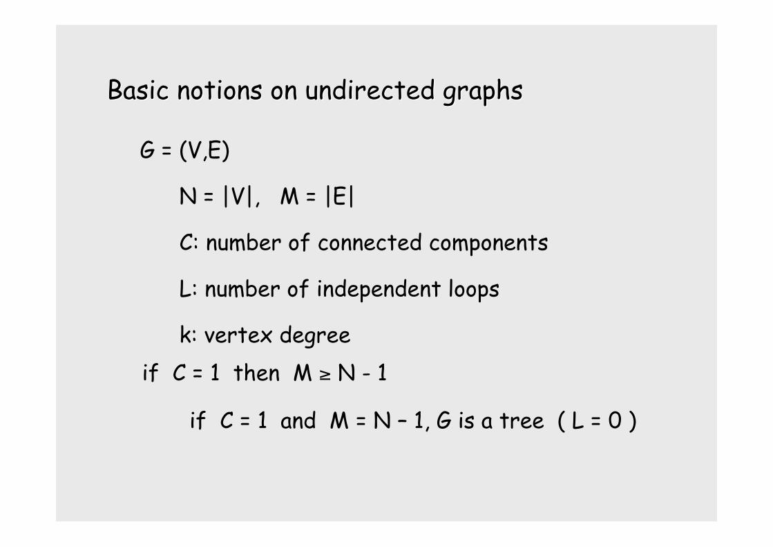
Basic notions on undirected graphsBasic notions on undirected graphs

G = (V,E)

N = |V|, M = |E|

C: number of connected components

L: number of independent loops

k: vertex degreeif C = 1 then M ≥ N - 1

if C = 1 and M = N – 1, G is a tree ( L = 0 )

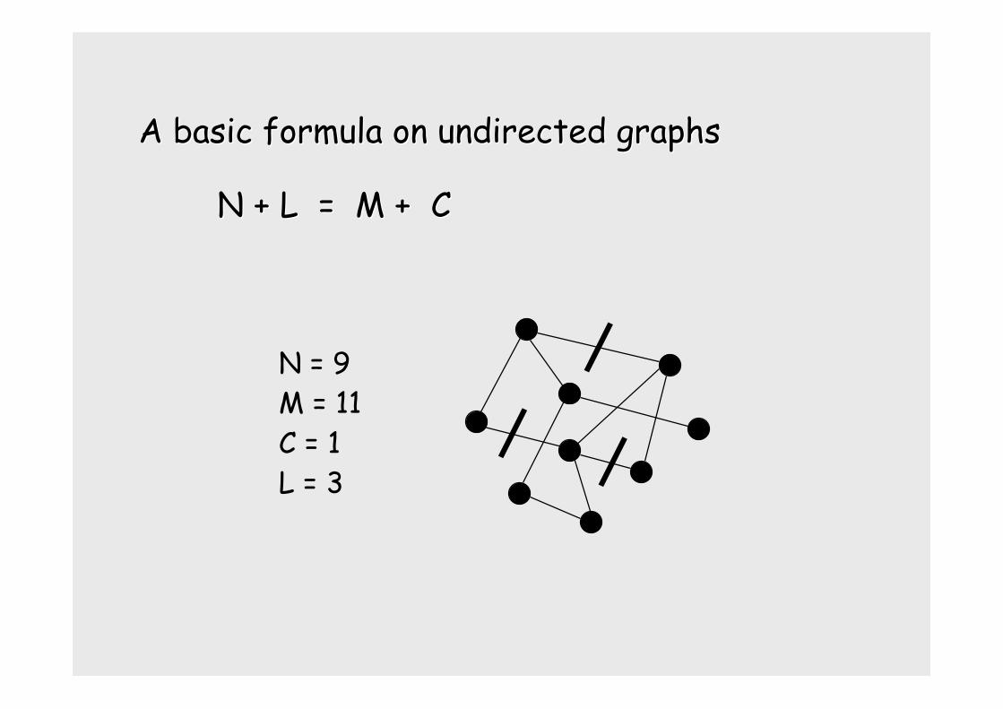
A basic formula on undirected graphsA basic formula on undirected graphs

N + L = M + CN + L = M + C

N = 9M = 11C = 1L = 3

Random networksRandom networks have a disorderedarrangement of edges.

A particular random network under study isonly one member of a statistical ensemblestatistical ensemble ofall possible realizations.

Therefore the statistical descriptionstatistical description of arandom network is in fact the description ofthe corresponding ensemble.

We shall study networks in the form ofgraphsgraphs (possibly, random graphs).

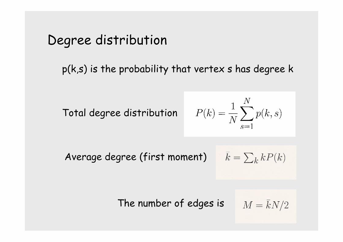
Degree distributionDegree distribution

p(k,s)p(k,s) is the probability that vertex s has degree kk

Total degree distributionTotal degree distribution

Average degreeAverage degree (first moment)

The number of edges is

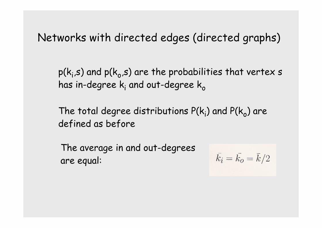
Networks with directed edges (directed graphs)Networks with directed edges (directed graphs)

p(kp(kii,s,s)) and p(kp(koo,s),s) are the probabilities that vertex sshas in-degree kkii and out-degree kkoo

The total degree distributions P(kP(kii)) and P(kP(koo)) aredefined as before

The average average in and out-degreesare equal:

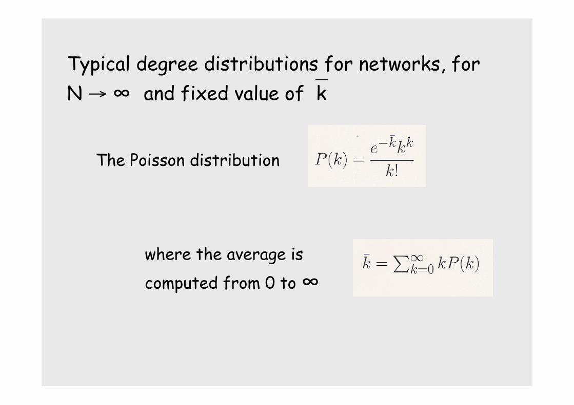
Typical degree distributions for networks, forN → ∞ and fixed value of k

The PoissonPoisson distribution

where the average average is

computed from 0 to ∞

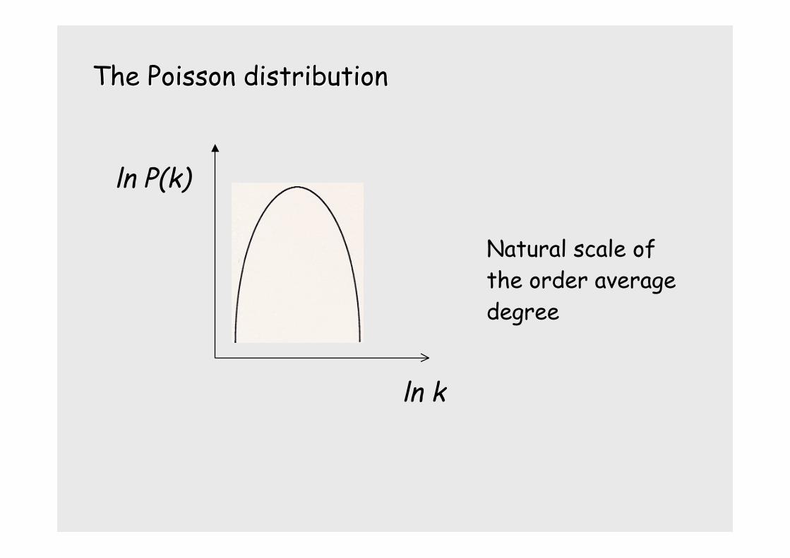
The Poisson distributionThe Poisson distribution

ln P(k)

ln k

Natural scale ofthe order averagedegree

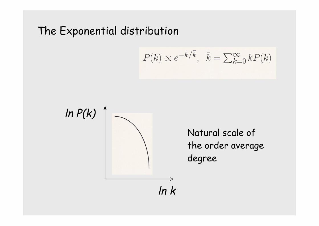
The Exponential distributionThe Exponential distribution

ln P(k)

ln k

Natural scale ofthe order averagedegree

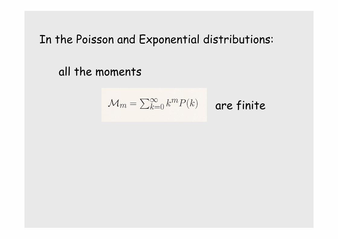
In the Poisson and Exponential distributions:In the Poisson and Exponential distributions:

all the moments

are finite

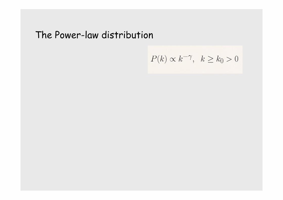
The Power-law distributionThe Power-law distribution

The Power-law distributionThe Power-law distribution

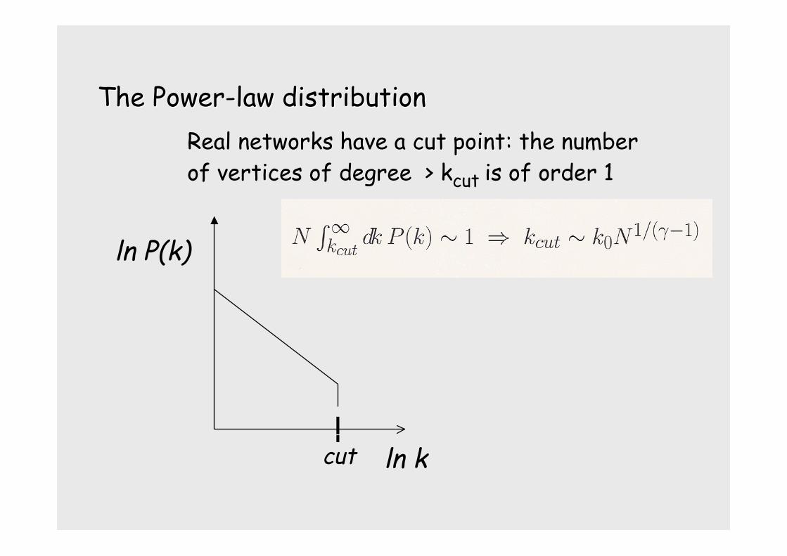
ln P(k)

ln kcut

Real networks have a cut pointcut point: the numberof vertices of degree > kcut is of order 1

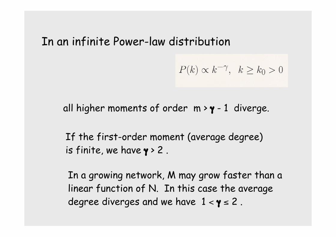
In an infinite Power-law distribution

all higher moments of order m > γ - 1 diverge.diverge.

If the first-order moment (average degree)is finiteis finite, we have γ > 2 .

In a growing network, M may grow faster than alinear function of N. In this case the averagedegree divergesdiverges and we have 1 < γ ≤ 2 .

Infinite power-laws are self-similarInfinite power-laws are self-similar

Self-similarity means that an infinite structure S and a part ofit appear to be the same. This entails the possibility of scaling,

In the Euclidean space a volume V scales with exponent+3 in the linear length L: a cube with V = L3 is still acube if the edge is doubled, L = 2L and V = 23 L3.

Fractals scale according to their non integer dimensions.

i.e., for S = S(x) we have S(cx) = c γ S(x) where c is a

constant and γ is the scaling exponent.

The only functions obeying this relationship are thepower-laws.

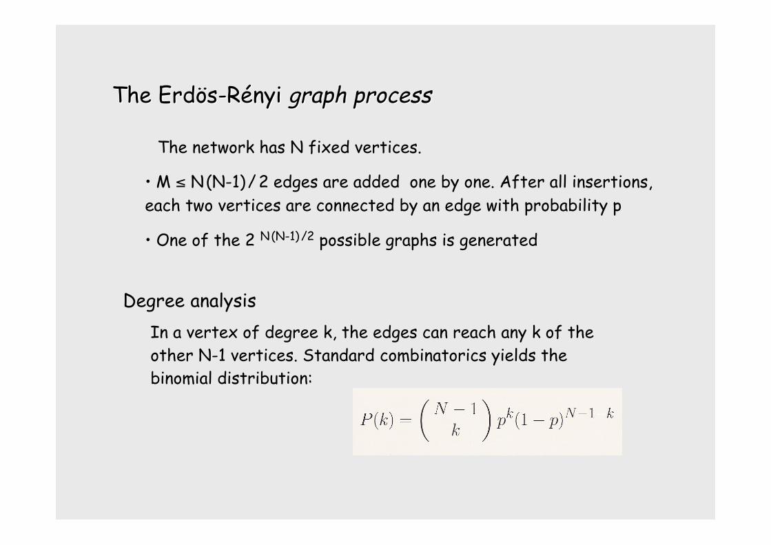
The The ErdErdööss--RRéényi nyi graph processgraph process

• The network has N fixed vertices.

• M ≤ N (N-1) / 2 edges are added one by one. After all insertions,each two vertices are connected by an edge with probability p

• One of the 2 N (N-1)

/2 possible graphs is generated

Degree analysisIn a vertex of degree k, the edges can reach any k of theother N-1 vertices. Standard combinatorics yields thebinomial distribution:

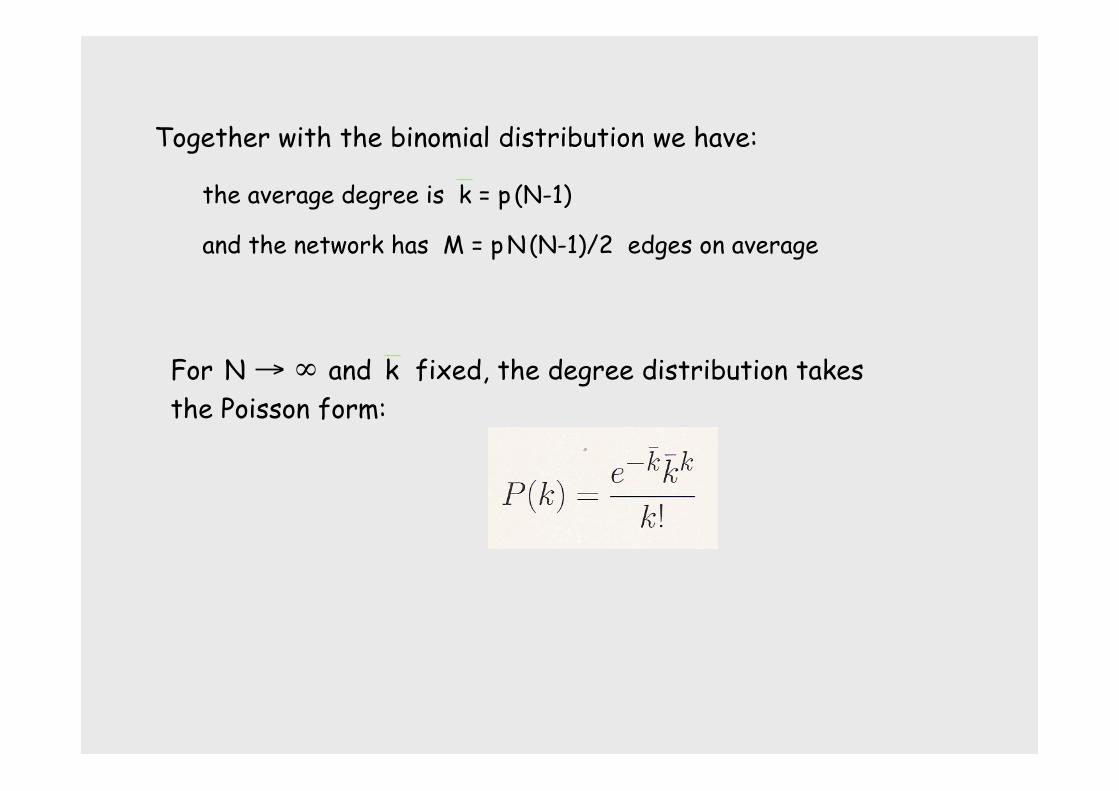
Together with the binomial distributiondistribution we have:

the average degree is k = p (N-1)

and the network has M = p N (N-1)/2 edges on average

For N → ∞ and k fixed, the degree distribution takesthe Poisson form:

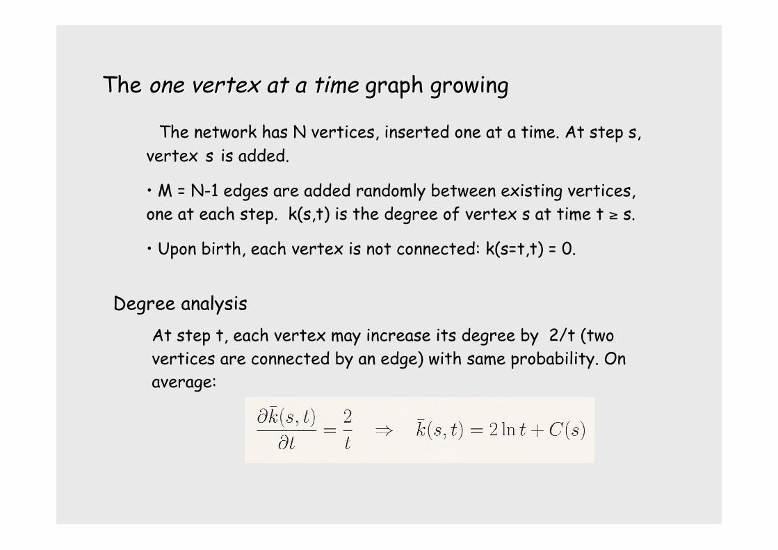
The The one vertex at a timeone vertex at a time graph growing graph growing

• The network has N vertices, inserted one at a time. At step s,vertex s is added.

• M = N-1 edges are added randomly between existing vertices,one at each step. k(s,t) is the degree of vertex s at time t ≥ s.

• Upon birth, each vertex is not connected: k(s=t,t) = 0.

Degree analysisAt step t, each vertex may increase its degree by 2/t (twovertices are connected by an edge) with same probability. Onaverage:

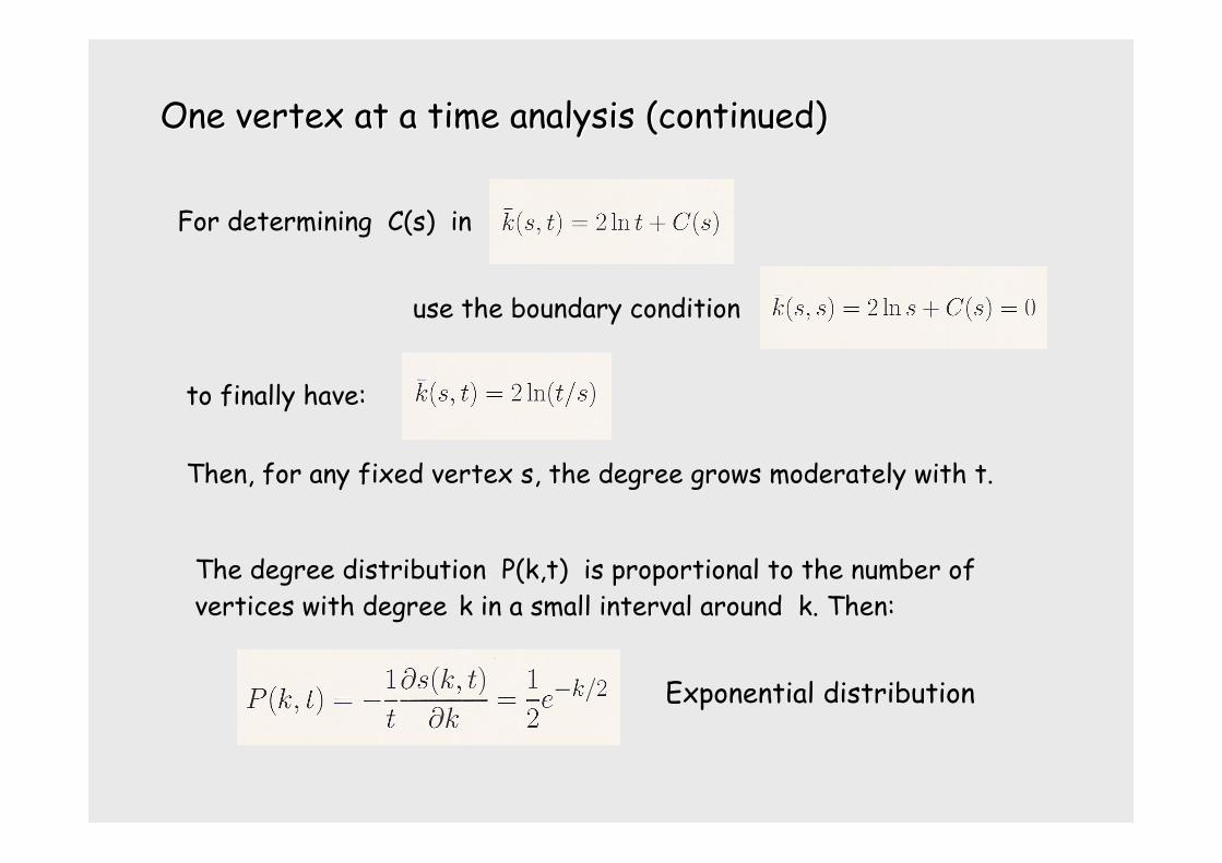
One vertex at a time analysis (continued)One vertex at a time analysis (continued)

to finally have:

For determining C(s) in

use the boundary condition

Then, for any fixed vertex s, the degree grows moderately with t.

The degree distribution P(k,t) is proportional to the number ofvertices with degree k in a small interval around k. Then:

Exponential distribution

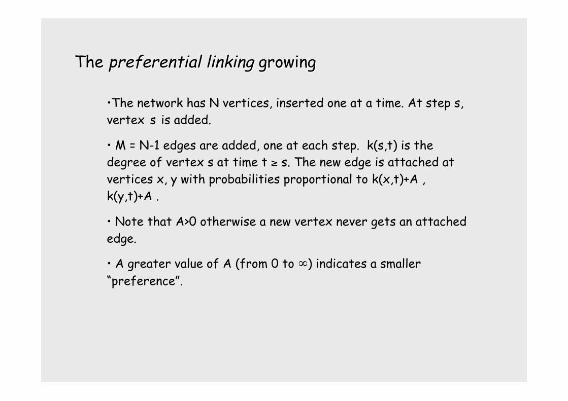
The The preferential linkingpreferential linking growing growing

•The network has N vertices, inserted one at a time. At step s,vertex s is added.

• M = N-1 edges are added, one at each step. k(s,t) is thedegree of vertex s at time t ≥ s. The new edge is attached atvertices x, y with probabilities proportional to k(x,t)+A ,k(y,t)+A .

• Note that A>0 otherwise a new vertex never gets an attachededge.

• A greater value of A (from 0 to ∞) indicates a smaller“preference”.

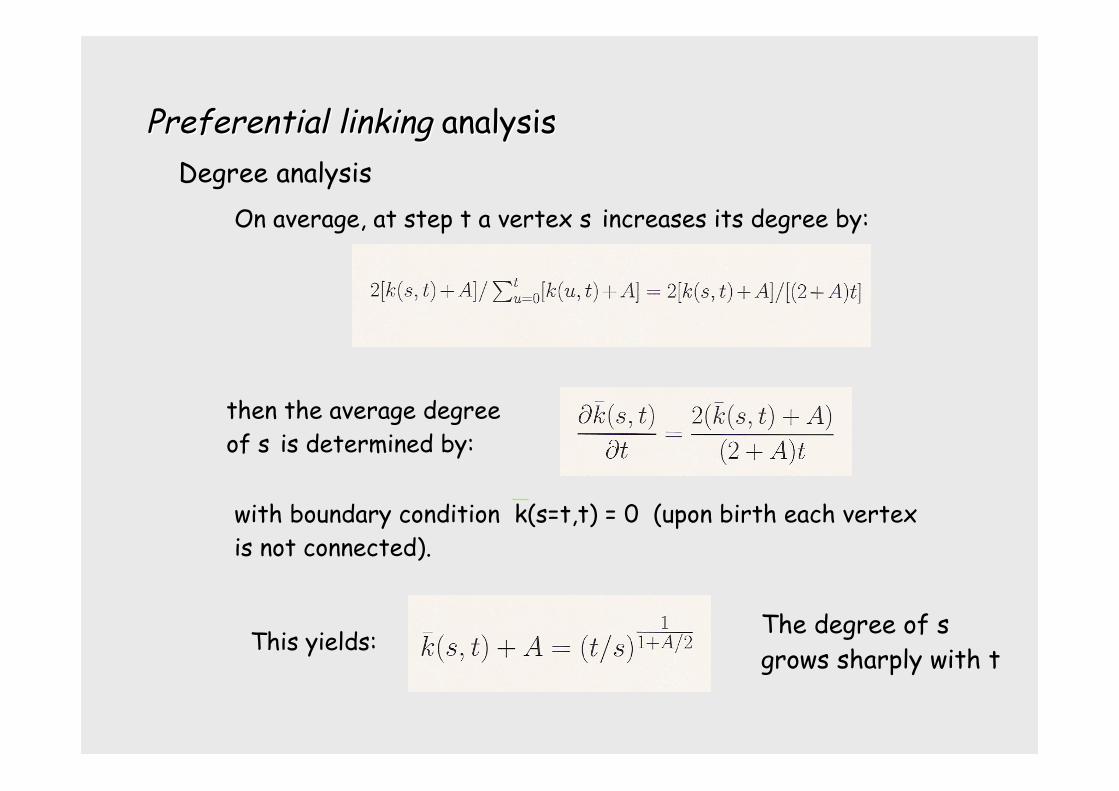
Preferential linkingPreferential linking analysis analysisDegree analysis

On average, at step t a vertex s increases its degree by:

then the average degreeof s is determined by:

with boundary condition k(s=t,t) = 0 (upon birth each vertexis not connected).

This yields:The degree of sgrows sharply with t

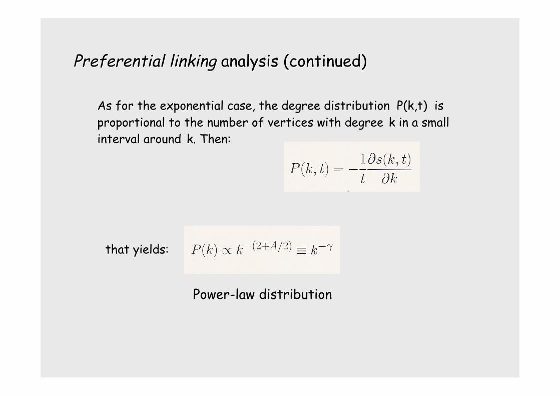
Preferential linkingPreferential linking analysis (continued) analysis (continued)

As for the exponential case, the degree distribution P(k,t) isproportional to the number of vertices with degree k in a smallinterval around k. Then:

Power-law distribution

that yields:

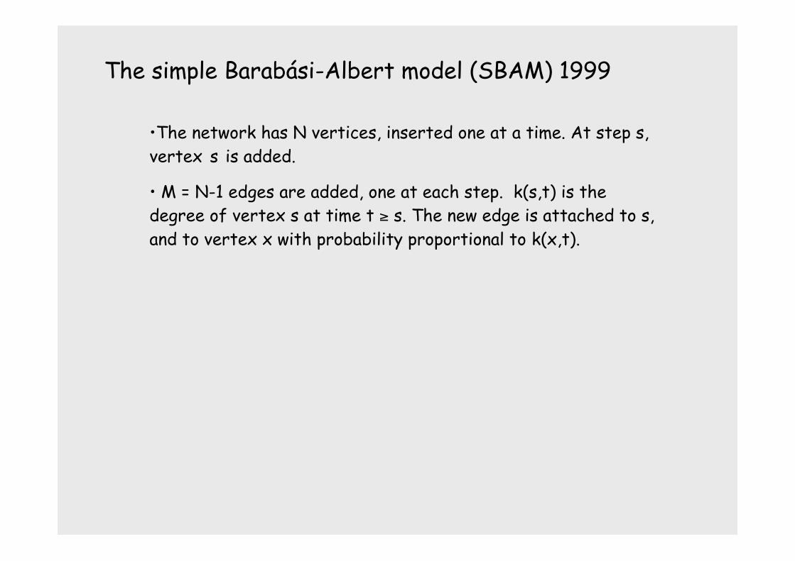
The simple Barabási-Albert model (SBAM) 1999

•The network has N vertices, inserted one at a time. At step s,vertex s is added.

• M = N-1 edges are added, one at each step. k(s,t) is thedegree of vertex s at time t ≥ s. The new edge is attached to s,and to vertex x with probability proportional to k(x,t).

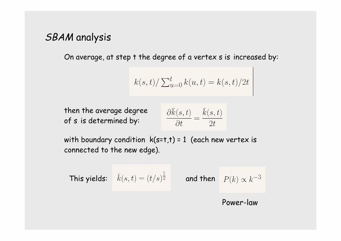
SBAMSBAM analysis analysis

On average, at step t the degree of a vertex s is increased by:

then the average degreeof s is determined by:

with boundary condition k(s=t,t) = 1 (each new vertex isconnected to the new edge).

This yields:

Power-law

and then

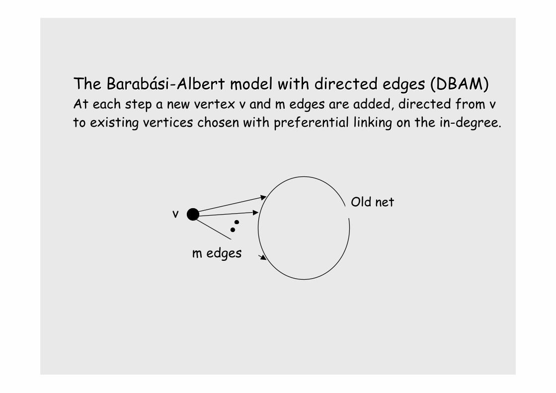
The The BarabBarabáásisi-Albert model with directed edges (DBAM)-Albert model with directed edges (DBAM)At each step a new vertex v and m edges are added, directed from vto existing vertices chosen with preferential linkingpreferential linking on the in-degree.

v

m edges

Old net

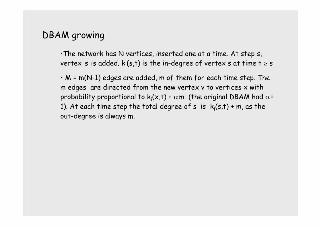
DBAM growingDBAM growing

•The network has N vertices, inserted one at a time. At step s,vertex s is added. ki(s,t) is the in-degree of vertex s at time t ≥ s

• M = m(N-1) edges are added, m of them for each time step. Them edges are directed from the new vertex v to vertices x withprobability proportional to ki(x,t) + α m (the original DBAM had α =1). At each time step the total degree of s is ki(s,t) + m, as theout-degree is always m.

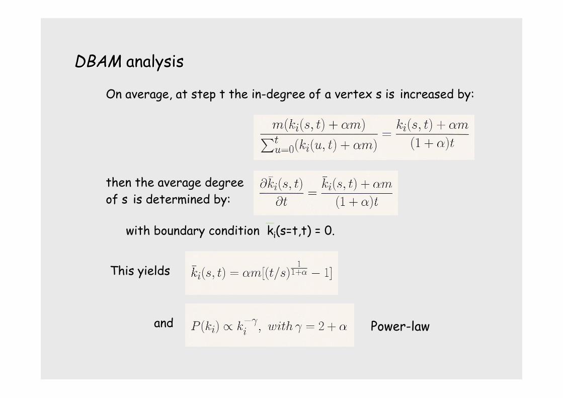
DBAMDBAM analysis analysis

On average, at step t the in-degree of a vertex s is increased by:

then the average degreeof s is determined by:

with boundary condition ki(s=t,t) = 0.

This yields

Power-lawand

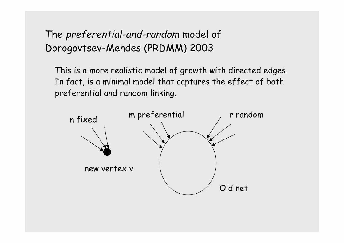
The The preferential-and-randompreferential-and-random model of model ofDorogovtsevDorogovtsev-Mendes (PRDMM) 2003-Mendes (PRDMM) 2003

new vertex v

m preferential

Old net

This is a more realistic model of growth with directed edges.In fact, is a minimal model that captures the effect of bothpreferential and random linking.

r randomn fixed

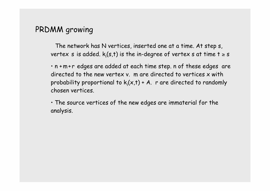
PRDMM growingPRDMM growing

• The network has N vertices, inserted one at a time. At step s,vertex s is added. ki(s,t) is the in-degree of vertex s at time t ≥ s

• n + m + r edges are added at each time step. n of these edges aredirected to the new vertex v. m are directed to vertices x withprobability proportional to ki(x,t) + A. r are directed to randomlychosen vertices.

• The source vertices of the new edges are immaterial for theanalysis.

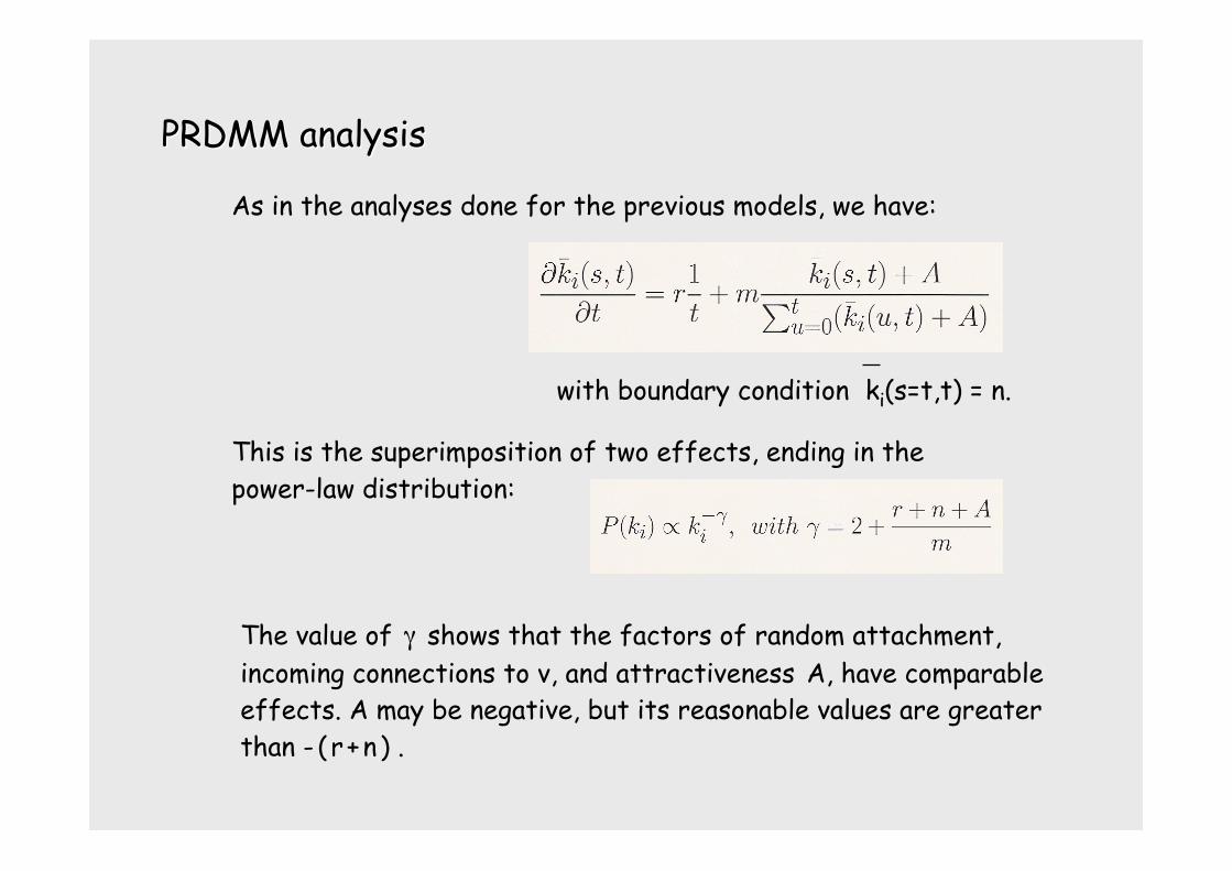
PRDMM analysisPRDMM analysis

As in the analyses done for the previous models, we have:

with boundary condition ki(s=t,t) = n.

This is the superimposition of two effects, ending in thepower-law distribution:

The value of γ shows that the factors of random attachment,incoming connections to v, and attractiveness A, have comparableeffects. A may be negative, but its reasonable values are greaterthan - ( r + n ) .

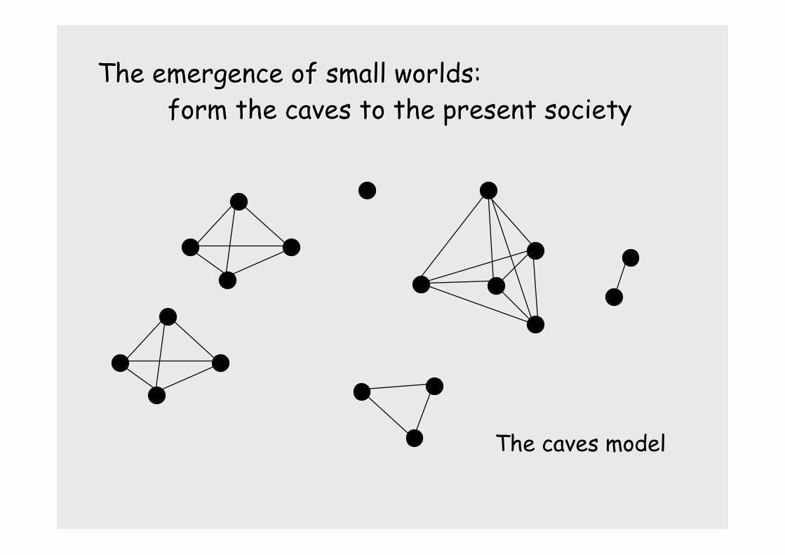
The emergence of small worlds:The emergence of small worlds: form the caves to the present society form the caves to the present society

The caves model

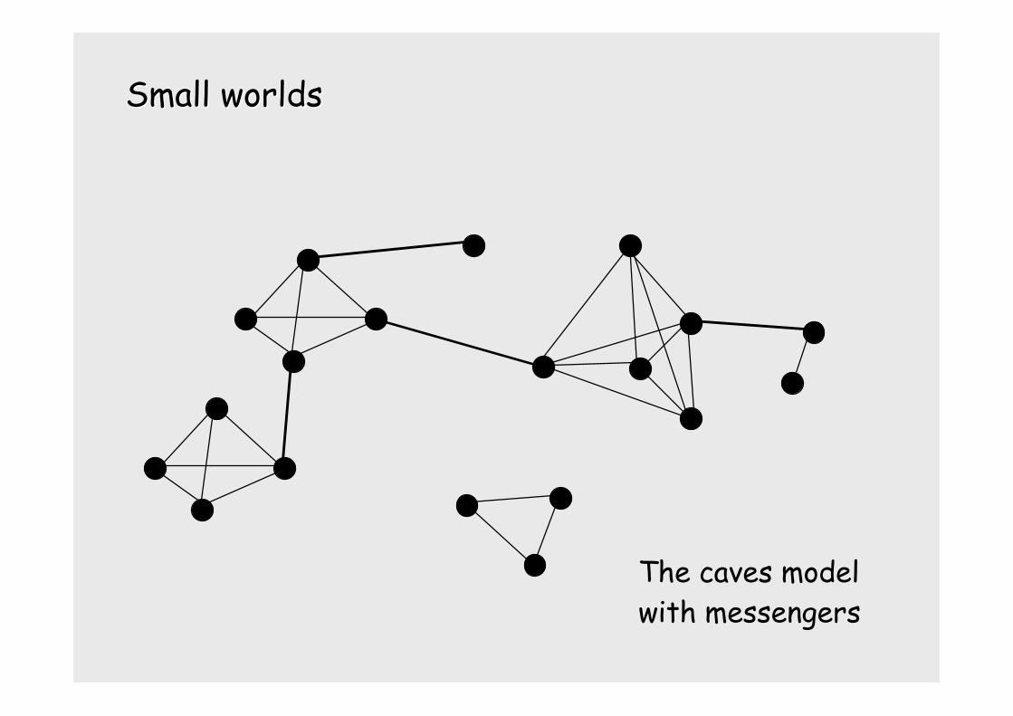
Small worldsSmall worlds

The caves modelwith messengers

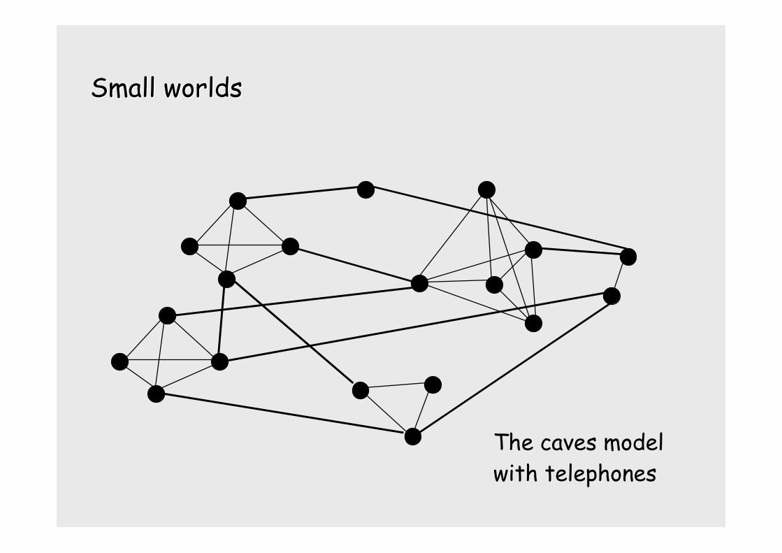
Small worldsSmall worlds

The caves modelwith telephones

Small worlds: vertex distanceSmall worlds: vertex distance

A key concept is the distancedistance between any twovertices x, y, i.e. the number of edges in theshortest pathshortest path between x and y

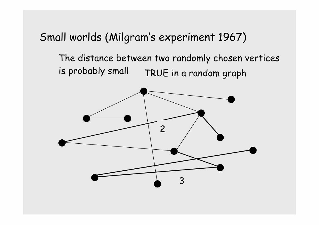
Small worlds (Small worlds (MilgramMilgram’’s s experiment 1967)experiment 1967)

The distance between two randomly chosen verticesis probably small

2

3

TRUE TRUE in a random graphin a random graph

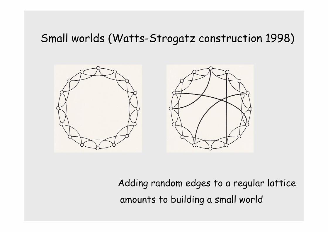
Small worlds (Watts-Small worlds (Watts-Strogatz Strogatz construction 1998)construction 1998)

Adding random edges to a regular latticeAdding random edges to a regular lattice

amounts to building a small worldamounts to building a small world

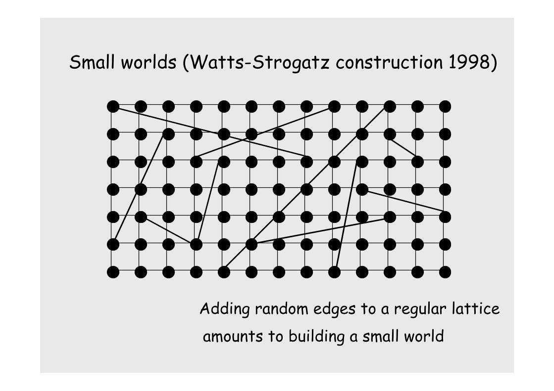
Small worlds (Watts-Small worlds (Watts-Strogatz Strogatz construction 1998)construction 1998)

Adding random edges to a regular latticeAdding random edges to a regular lattice

amounts to building a small worldamounts to building a small world

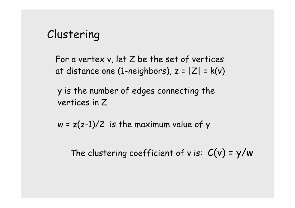
ClusteringClustering

The clustering coefficientclustering coefficient of v is: C(v) = y/wC(v) = y/w

For a vertex v, let Z be the set of verticesat distance one (1-neighbors1-neighbors), z = |Z| = k(v)

y is the number of edges connecting thevertices in Z

w = z(z-1)/2 is the maximum value of y

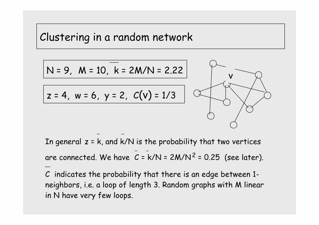
Clustering in a random networkClustering in a random network

v

z = 4, w = 6, y = 2, CC(v)(v) = 1/3 = 1/3

N = 9, M = 10, k = 2M/N = 2.22

In general z = k, and k/N is the probability that two vertices

are connected. We have C = k/N = 2M/NC = k/N = 2M/N 22 = 0.25 = 0.25 (see later).

C indicates the probability that there is an edge between 1-neighbors, i.e. a loop of length 3. Random graphs with M linearin N have very few loops.

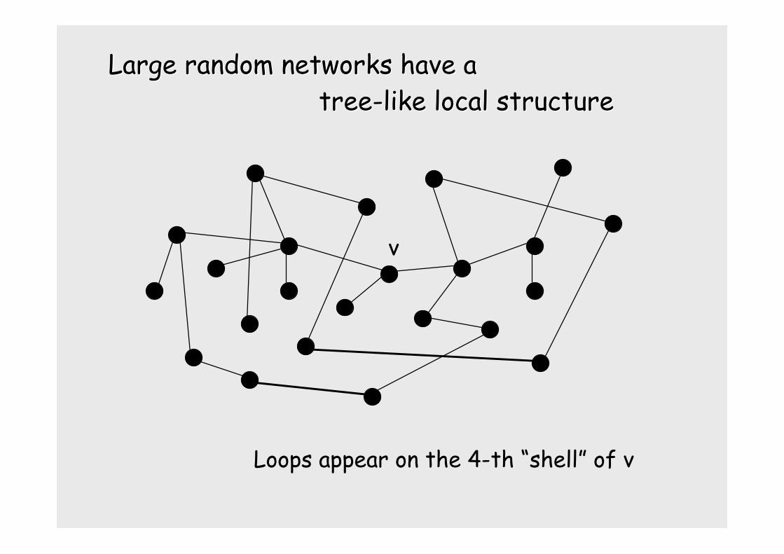
Large random networks have aLarge random networks have a tree-like local structure tree-like local structure

v

Loops appear on the 4-th “shell” of v

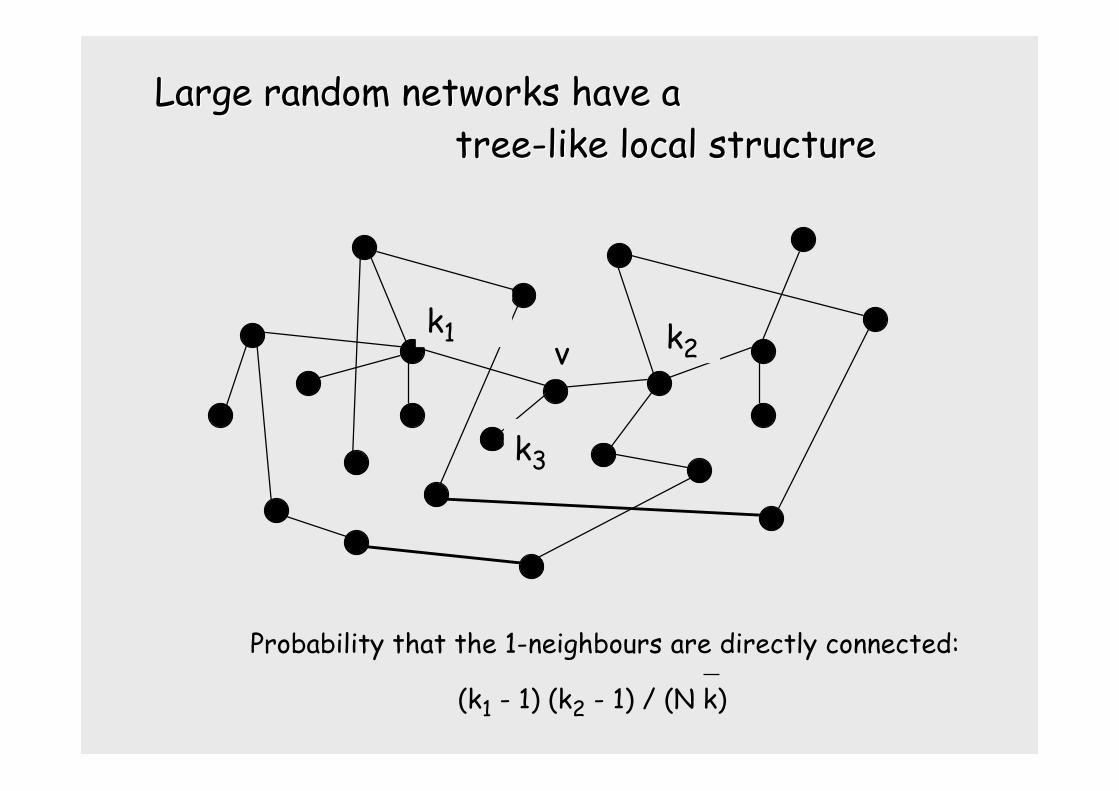
Large random networks have aLarge random networks have a tree-like local structure tree-like local structure

vk1 k2

k3

Probability that the 1-neighbours are directly connected:

(k1 - 1) (k2 - 1) / (N k)

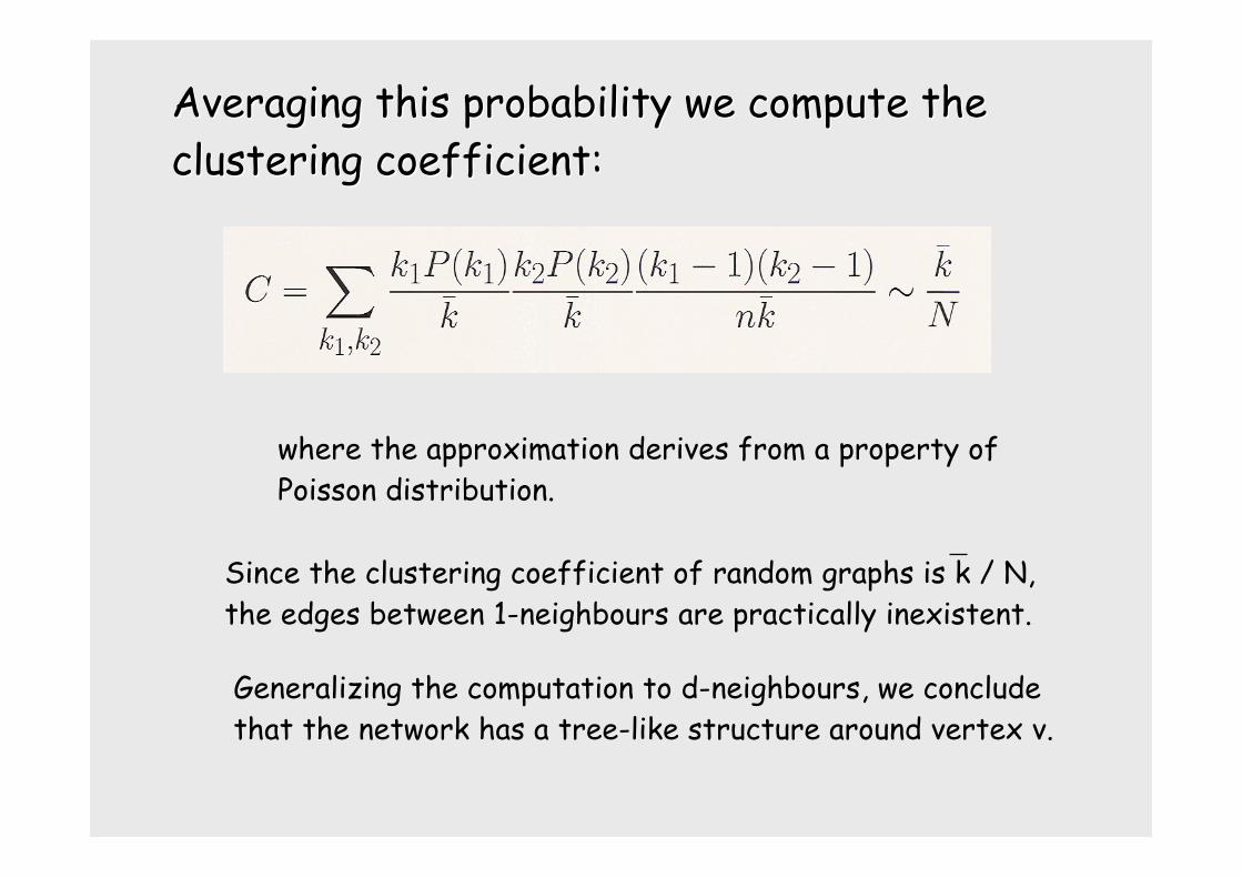
Averaging this probability we compute theAveraging this probability we compute theclustering coefficient:clustering coefficient:

where the approximation derives from a property ofPoisson distribution.

Since the clustering coefficient of random graphs is k / N,the edges between 1-neighbours are practically inexistent.

Generalizing the computation to d-neighbours, we concludethat the network has a tree-like structure around vertex v.

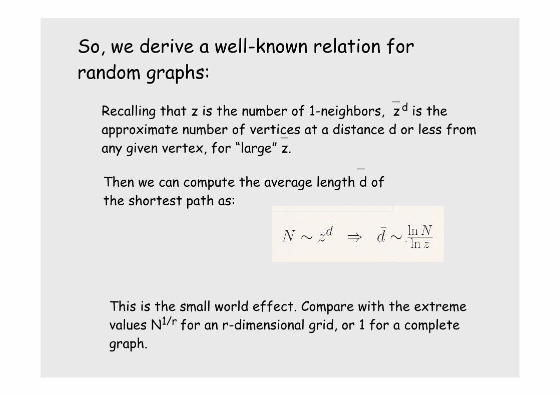
So, we derive a well-known relation forSo, we derive a well-known relation forrandom graphs:random graphs:

This is the small world effect. Compare with the extremevalues N1/r for an r-dimensional grid, or 1 for a completegraph.

Recalling that z is the number of 1-neighbors, z d is the

approximate number of vertices at a distance d or less fromany given vertex, for “large” z.

Then we can compute the average length d ofthe shortest path as:

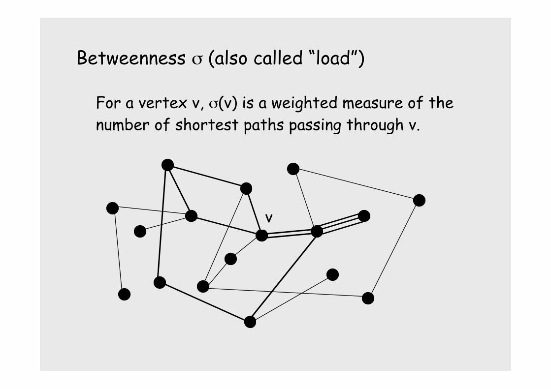
Betweenness Betweenness σ (also called (also called ““loadload””))

v

For a vertex v, σ(v) is a weighted measure of thenumber of shortest paths passing through v.

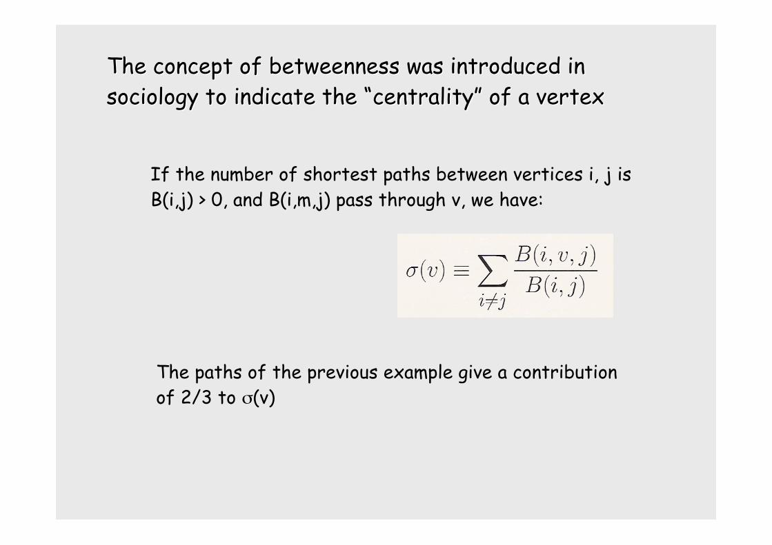
The concept of The concept of betweenness betweenness was introduced inwas introduced insociology to indicate the sociology to indicate the ““centralitycentrality”” of a vertex of a vertex

If the number of shortest paths between vertices i, j isB(i,j) > 0, and B(i,m,j) pass through v, we have:

The paths of the previous example give a contributionof 2/3 to σ(v)

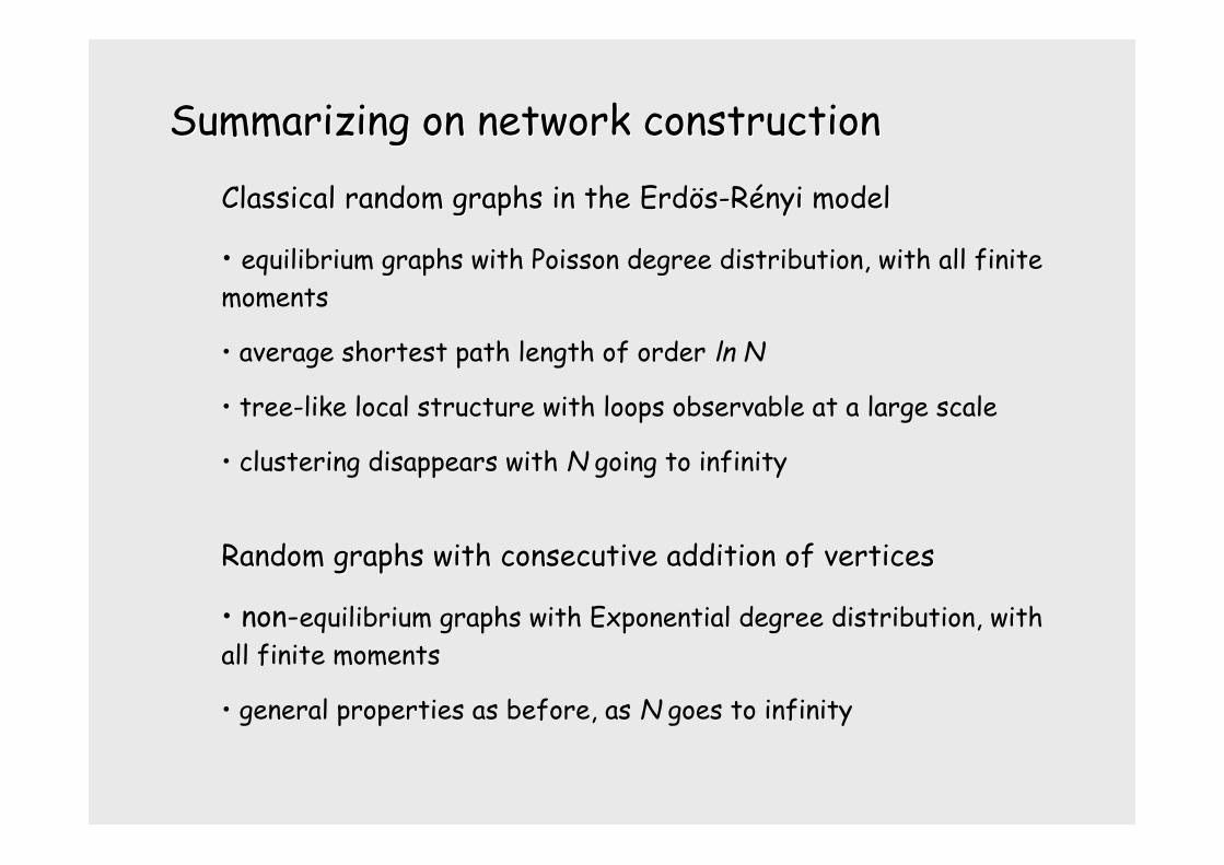
Summarizing on network constructionSummarizing on network construction

Classical random graphs in the Classical random graphs in the ErdErdööss--RRéényi nyi modelmodel

• equilibrium graphs with Poisson degree distribution, with all finitemoments

• average shortest path length of order ln N

• tree-like local structure with loops observable at a large scale

• clustering disappears with N going to infinity

Random graphs with consecutive addition of verticesRandom graphs with consecutive addition of vertices

• non-equilibrium graphs with Exponential degree distribution, withall finite moments

• general properties as before, as N goes to infinity

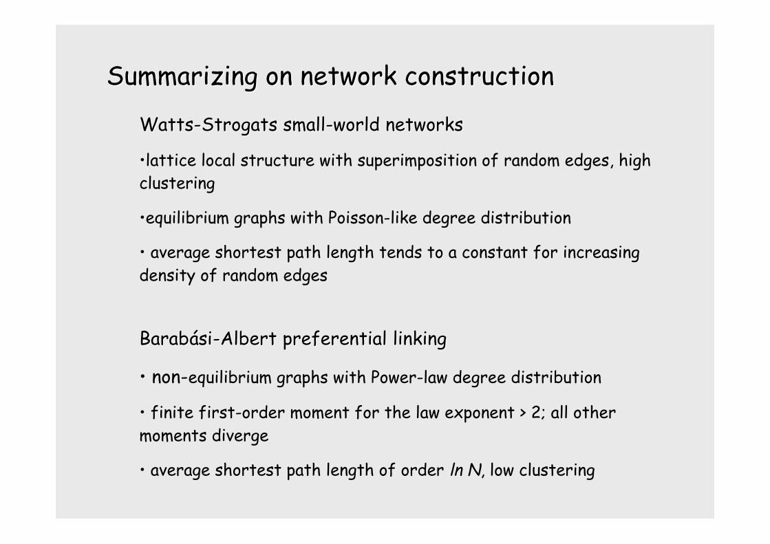
Summarizing on network constructionSummarizing on network construction

Watts-Watts-Strogats Strogats small-world networkssmall-world networks

•lattice local structure with superimposition of random edges, highclustering

•equilibrium graphs with Poisson-like degree distribution

• average shortest path length tends to a constant for increasingdensity of random edges

BarabBarabáásisi-Albert preferential linking-Albert preferential linking

• non-equilibrium graphs with Power-law degree distribution

• finite first-order moment for the law exponent > 2; all othermoments diverge

• average shortest path length of order ln N, low clustering

A fundamental book for startingA fundamental book for starting

S.R. Dogorovtsev, J.F.F. MendesS.R. Dogorovtsev, J.F.F. Mendes. Evolution of Networks.. Evolution of Networks.Oxford University Press 2003.Oxford University Press 2003.

many formulae in this section are taken from it