Embed Size (px)
Citation preview
Volkswirtschaftliche DiskussionsbeiträgeVolkswirtschaftliche Diskussionsbeiträge
U N I K a s s e lV E R S I T Ä T
FachbereichWirtschaftswissenschaften
Factor Analysis Regression
von
Reinhold Kosfeld und Jorgen Lauridsen
Nr. 57/04
Factor Analysis Regression Reinhold Kosfeld1 and Jorgen Lauridsen2 1 University of Kassel, Department of Economics, Nora-Platiel-Str. 5, D-34117 Kassel, Germany, E-Mail: [email protected] 2 University of Southern Denmark, Department of Economics, Campusvej 55, DK-5230 Odense M, Denmark, E-Mail: [email protected] Abstract. In presence of multicollinearity principal component regression (PCR) is sometimes suggested for the estimation of the regression coefficients of a multiple regression model. Due to ambiguities in the interpretation involved by the orthogonal transformation of the set of explanatory variables the method could not yet gain wide acceptance. Factor analysis regression (FAR) provides a model-based estimation method which is particular tailored to overcome multicollinearity in an errors in variables setting. In this paper we present a new FAR estimator that proves to be unbiased and consistent for the coefficient vector of a multiple regression model given the parameters of the measurement model. The behaviour of feasible FAR estimators in the general case of completely unknown model parameters is studied in comparison with the OLS estimator by means of Monte Carlo simulation. JEL C13, C20, C51 Keywords: Factor Analysis Regression, Multicollinearity, Factor model, Errors in Variables 1. Introduction In case of multicollinearity the identification of separate influences of highly collinear
variables proves to be extremely difficult. Due to negative covariances of estimated regression
coefficients an overrating of one regression coefficient is known to go along with an
underrating of another when standard estimation methods are applied. Only the common
influence of the regressors can be reliable estimated. This issue is highly relevant for testing
hypotheses and evaluating policy measurements.
Several suggestions have been made to employ the methods of principal components in case
of highly correlated explanatory variables in a multiple regression model in order to overcome
- or at least mitigate - the problem of multicollinearity, see e.g. Amemiya (1985; pp. 57),
Fomby et al. (1988, pp. 298). With principal components regression (PCR) one is willing to
accept a biased estimation of the regression coefficients for the sake reduction of variability.
However, due to ambiguities in the interpretation involved by the orthogonal transformation
PCR could not gain wide acceptance, see Greene (2003, pp. 58).
Factor analysis regression (FAR) provides a model-based estimation method that is particular
tailored to cope with multicollinearity in an errors in variables setting. Scott (1966, 1969) was
the first to address this issue by deriving “factor analysis regression equations” from a factor
2
model of both the dependent and the explanatory variables. The theoretical deficiencies of
Scott’s approach are criticized for the most part by King (1969).1 He showed that Scott’s FAR
estimator is biased and that the bias still exists asymptotically. Scott’s FAR approach has been
reconsidered by Lawley and Maxwell (1973), Chan (1977) and Isogawa and Okamoto (1980).
Chan’s investigation focuses on how to overcome the inconsistency in predicting the
dependent variable in this type of FAR model , see also Basilevsky (1994, pp. 694).
Basilevsky (1981) has developed an FAR estimator based on a factor analysis of only the
explanatory variables. This approach of factor analysis regression gets particular attraction as
it is the dependencies across the explanatory variables that are responsible for
multicollinearity. Given the parameters of the multiple factor model Basilevsky’s FAR
estimator proves to be unbiased and consistent, see Basilevsky (1981) and Basilevsky (1994,
pp. 672). The finite-sample sample properties are, however, completely unknown for any kind
of FAR estimator.
The present paper aims at closing this gap. In section 2 the latter kind of the FAR approach is
outlined. We distinguish two types of FAR estimators. The FAR estimator of first type is
attached to the common factors, while the FAR estimator of second type refers to the “true” in
the sense of flawless measured explanatory variables. An FAR estimator derived in this
context differs from Basilevsky’s proposal in respect to its entirely data-based design. In
section 3.1 it is shown that new FAR estimator shares the properties of the Basilevsky
estimator under the same set of assumptions. The finite-sample properties of two feasible
FAR estimators are investigated by Monte Carlo simulation in section 3.2. Special features of
FAR estimators disclosed by the simulation experiments are discussed. Section 4 concudes
with some qualifications regarding the applicability of the FAR approach.
2. FAR model and estimation
Let y be an nx1 vector of the regressand y, Ξ an nxp matrix of the stationary regressors ξj
measured as deviations from their means, β a px1 vector of the regression coefficients βj and
v an nx1 vector of disturbances v. Further assume that the structural equation of an
econometric model is given by the multiple regression equation 1 There still exist some additional problems with Scott’s FAR approach. His so-called “factor analysis regression
equations” e.g. do not result from a transformation of the factor matrix to a more simple and better interpretative structure in the sense of Thurstone’s concept of simple structure (Thurstone, 1970). It is simply the result of a reduction of multiple factor model to a one factor model. A “rotation” of the factor matrix is unnecessary since the implied “regression coefficients” are invariant to orthogonal transformations.
3
(2.1) y = Ξ⋅β + v.
The regressors ξj, however, are prone to measurement errors uj and thence are not directly
observable. Only their flawed counterparts xj, ξj + uj, are accessible to observation. Hence, the
nxp observation matrix X is composed of the matrix of “true” regressor values, Ξ, and the nxp
matrix of measurement errors, U:
(2.2) X = Ξ + U.
By substituting Ξ with X-U in Equation (2.1) one obtains the error in variables model
(2.3) y = X⋅β + ε
with the error term
(2.4) ε = v - U⋅β.
It is well-known that the properties of the OLS estimator for the parameter
vector β depend on the kind of relationship among the regressors and the disturbances. If
Equation (2.1) renders the “true” regression for which the standard assumptions
yXXXβ ')'(ˆ 1−=
(2.5) (a) E(vΞ) = o and (b) Σv = E(v⋅v’Ξ) = ⋅I2vσ n
hold, it follows that the flawed regressors xj in model (2.3) are correlated with the
disturbances εj. In this case the OLS estimator β is neither unbiased nor consistent for β.
Since the bias depends on the ratio σ (Johnston and DiNardo, 1997, pp. 153), it may be
negligible in situations when the disturbance variance σ is small with regard to the variance
of the true regressors. Here we refer to the case of multicollinearity where the OLS
estimator is bound up with high variability. Moreover, an overrating of one regression
coefficient is known to come along with an underrating of another one. With increasing
correlations the explonatory variables share larger common parts which makes a separation of
their influences on the dependent variable more and more difficult.
ˆ
22v / ξσ
2v
2ξσ
From experience with principal components regression it can be expected that variability
generally could be reduced by orthogonalising the collinear regressors. However, the increase
of the bias with the orthogonalisation transformation has turned out to be dramatic.2 The
advantage of factor analysis regression consists in explicitly allowing for the model structure.
2 This conclusion is drawn from an own simulation study which cannot be presented here due to space limitation.
4
Factor analysis serves as a measurement model for the common and specific parts of the
regressors. After extracting common factors in the first step, the dependent variable y is
regressed on the orthogonal factors f1, f2, …, fm in a second step (FAR estimator of 1st type).
In a third step a factor analysis regression estimator (FAR estimator of 2nd type) is derived
from the estimated influences of the factors on the explanatory and dependent variable y.
By using the multiple factor model (Dillon and Goldstein, 1984, pp. 53; Johnson and
Wichern, 1992, pp. 396)
(2.6) X = F⋅Λ’ + U
as a measurement model we assume a special data generating process for the explanatory
variables. According to the factor model (2.6) the observed explanatory variables are
generated by m common factors fk, m<p, and m specific factors uj. Each common factor is
associated with more than one explanatory variable, whereas the specific factors are exactly
assigned to a particular regressor. The specific factors match exactly with the measurement
errors uj in Equation (2.2). With
(2.7) Ξ = F⋅Λ’
the “true” regressors ξj are given by a linear combination of the common factors f1, f2, …, fm
which are arranged in the nxm factor score matrix F. The weights λjk of the linear combinat-
ion (2.7) are called factor loadings; the pxm matrix of the factor loadings, Λ, denotes the
factor matrix.
Without loss of generality
(2.8) E(F) = E(U) = 0
and
(2.9) Σf = E(n1 F’F) = Im
can be assumed. The assumption (2.9) of uncorrelated common factors fk is always necessary
for factor extraction. Although it can be altered in a later step it is retained in our case. The
covariance matrix of the unique factors uj must be diagonal:
(2.10) Σu = diag( ... ). 2u1
σ 2u 2
σ 2u p
σ
Note that the distinction of two kind of factors requires the common factors fk to be
uncorrelated with the specific factors uj:
5
(2.11) E(F’U) = 0.
Finally, we assume the common and unique factors to be independently normally distributed
with zero expectation and covariance matrices given by (2.9) and (2.10), respectively.
By inserting the hypothesis (2.7) on the generation of “true” regressors into the multiple
regression equation (2.1) one obtains
y = F⋅Λ’ ⋅β + v
or, with
(2.12) β* = Λ‘⋅β
(2.13) y = F⋅β* + v.
Equation (2.13) can be interpreted as a factor regression where the endogenous variable of the
original model, y, is explained by a set of common factors f1, f2, …, fm. While the explanatory
variables x1, x2, …, xp will be highly correlated in case of multicollinearity, the common
factors f1, f2, …, fm are uncorrelated. If the factor scores were assumed to be known, OLS
applied on (2.13) would produce the factor analysis regression (FAR) estimator with respect
to the common factors f1, f2, …, fm (FAR estimator of 1st type):
(2.14) = (F’⋅F)*FARβ̂ -1⋅F’⋅y.
Of course, since the common factors are not directly observable, they have to be estimated in
advance in order to measure the influences the common factors on the variable to be
explained in the model.
At the outset, though, we our interest has been addressed to the issue of a stable estimation of
the parameter vector β in case of multicollinearity. This type of factor analysis regression
(FAR) estimator (FAR estimator of 2nd type) has to capture the influences of the “true”
regressors ξ1, ξ2, …, ξp on the dependent variable y. To obtain an FAR estimator β for β
compatible to , the relationship (2.12) between the parameter vectors β* and β has to be
translated to both FAR estimators:
FARˆ
*FARβ̂
(2.15) = Λ’⋅β . *FARβ̂ FAR
ˆ
After substitution of in Equation (2.15) by (2.14) and premultiplication by the factor
matrix Λ, the relation
*FARβ̂
6
(2.16) Λ⋅Λ’⋅ = Λ⋅(F’⋅F)FARβ̂ -1⋅F’⋅y
results. The FAR estimator with respect to the explanatory variables ξ1, ξ2, …, ξp is then
given by
(2.17) ⋅β = (Λ⋅Λ’)FARˆ +⋅Λ⋅(F’⋅F)-1⋅F’⋅y,
where (Λ⋅Λ’)+ denotes the Moore-Penrose pseudo inverse of the product matrix Λ⋅Λ’. By
replacing y by (2.13) it is easily shown with (2.12) that the FAR estimator (2.17) is invariant
to orthogonal transformations of the factor matrix. Hence, the rotation problem of factor
analysis does not matter at all in factor analysis regression.
Note that in (2.17) both the factor matrix Λ and the factor score matrix F are unknown. In
order to determine the FAR estimator numerically, Λ and F have to be estimated in advance.
An orthogonal estimator of F is generally obtained, when Λ is estimated by maximum
likelihood or generalised least squares factor analysis, see Jöreskog (1977). In ML factor
analysis the relation
(2.18) IFF =⋅ ˆ'ˆn1
is met – in contrary to other extraction methods - not only approximately but exactly.
Moreover, ML factor analysis is preferable as well in order to ensure the consistency of an
estimator for the factor matrix Λ. To avoid a stodgy notation always denote a consistent
estimator of Λ. Then a feasible FAR estimator of type (2.17) reads
Λ̂ Λ̂
(2.19) .'ˆ)ˆ'ˆ(ˆ)'ˆˆ(ˆ̂ 1FAR yFFFΛΛΛβ ⋅⋅⋅⋅⋅= −+
The factor scores can be estimated by the well-known “regression estimator” (Thomson
estimator)
(2.20) '')'(')'('ˆ 12/1u
1u
'T XΛΛΣΛIXΣΛΛΛF ⋅+=+⋅= −−−
that is known to be a biased minimum variance estimator, see Brachinger and Ost (1996, pp.
691). Alternatively, the Bartlett estimator
(2.21) '')'(ˆ 2/1u
12/1u
'B XΣΛΛΣΛF −−−=
7
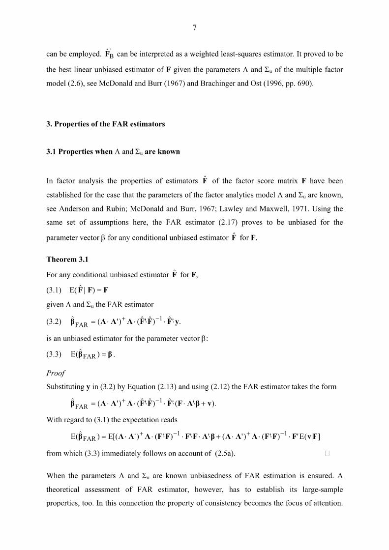
can be employed. can be interpreted as a weighted least-squares estimator. It proved to be
the best linear unbiased estimator of F given the parameters Λ and Σ
'BF̂
u of the multiple factor
model (2.6), see McDonald and Burr (1967) and Brachinger and Ost (1996, pp. 690).
3. Properties of the FAR estimators
3.1 Properties when Λ and Σu are known
In factor analysis the properties of estimators F of the factor score matrix F have been
established for the case that the parameters of the factor analytics model Λ and Σ
ˆ
u are known,
see Anderson and Rubin; McDonald and Burr, 1967; Lawley and Maxwell, 1971. Using the
same set of assumptions here, the FAR estimator (2.17) proves to be unbiased for the
parameter vector β for any conditional unbiased estimator for F. F̂
Theorem 3.1
For any conditional unbiased estimator for F, F̂
(3.1) E( | F) = F F̂
given Λ and Σu the FAR estimator
(3.2) .'ˆ)ˆ'ˆ()'(ˆ 1FAR yFFFΛΛΛβ ⋅⋅⋅⋅⋅= −+
is an unbiased estimator for the parameter vector β:
(3.3) . ββ =)ˆ(E FAR
Proof
Substituting y in (3.2) by Equation (2.13) and using (2.12) the FAR estimator takes the form
).'('ˆ)ˆ'ˆ()'(ˆ 1FAR vβΛFFFFΛΛΛβ +⋅⋅⋅⋅⋅⋅⋅= −+
With regard to (3.1) the expectation reads
](E')'()'('')'()'[(E)ˆ(E 11FAR FvFFFΛΛΛβΛFFFFΛΛΛβ ⋅⋅⋅⋅+⋅⋅⋅⋅⋅⋅⋅= −+−+
from which (3.3) immediately follows on account of (2.5a).
When the parameters Λ and Σu are known unbiasedness of FAR estimation is ensured. A
theoretical assessment of FAR estimator, however, has to establish its large-sample
properties, too. In this connection the property of consistency becomes the focus of attention.
8
Since unbiasedness also holds for n→∞, it is sufficient for β to be consistent for β to
show that its variances and covariances vanish asymptotically, see Judge et al. (1988, pp. 83
and p.260). With regard to Theorem (3.1) consistency is ensured if the covariance
matrix of β , Cov(β ), does approach a pxp zero matrix 0
FARˆ
FARβ̂
FARˆ
FARˆ p as n goes to infinity.
Theorem 3.2
For an asymptotical conditional unbiased estimator for F F̂
(3.4) E( | F) = F ∞→n
lim F̂
the FAR estimator (3.2) is a consistent estimator for the parameter vector β:
(3.5) ββ =∞→
FARn
ˆlimp .
given the parameters Λ and Σu
Proof
On account of Theorem (3.1) consistency of the FAR estimator β is ensured if its
covariance matrix Cov(β ) is proved to approach the zero matrix 0
FARˆ
FARˆ̂
p for n→∞.
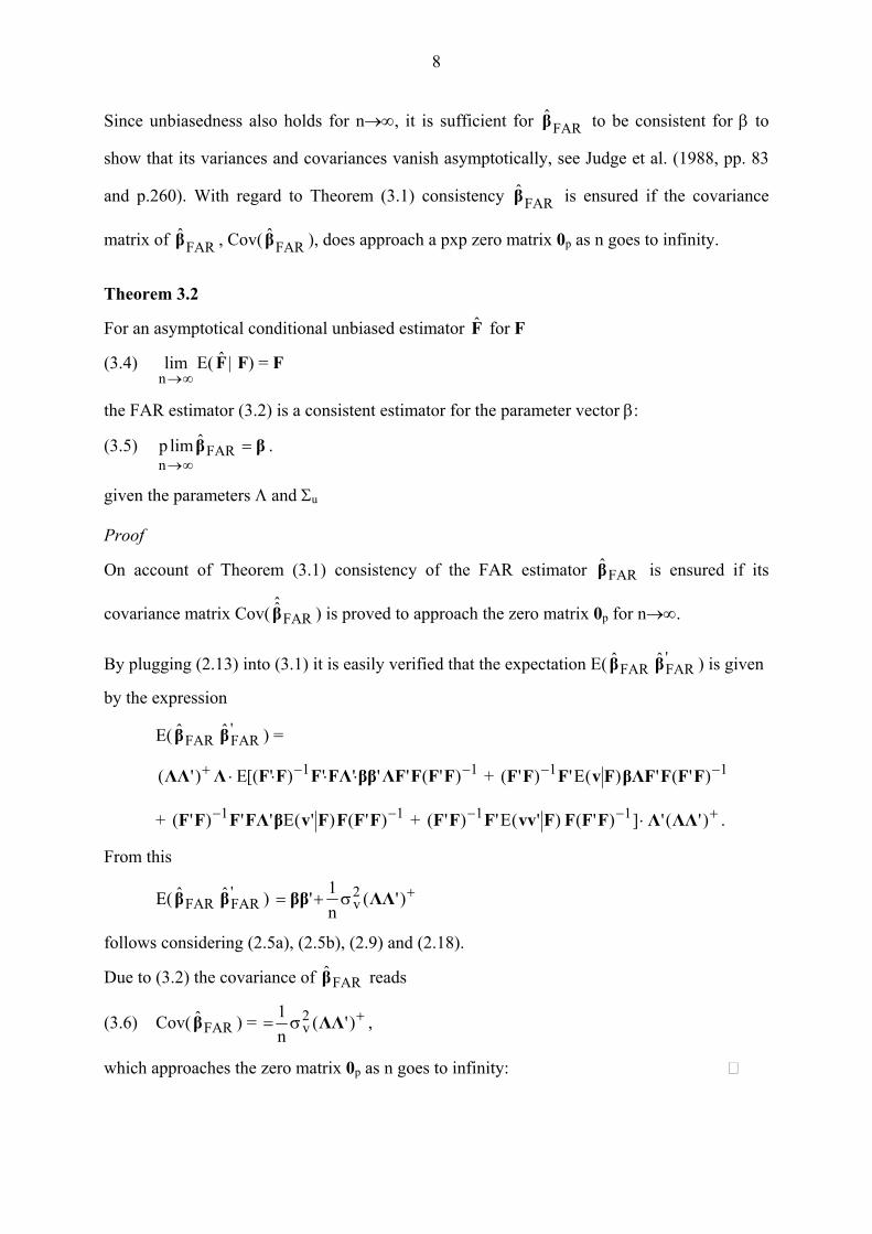
By plugging (2.13) into (3.1) it is easily verified that the expectation E(β ) is given
by the expression
FARˆ 'FARβ̂
E(β ) = FARˆ 'FARβ̂
11 )'('''')'[(E)'( −−+ ⋅⋅⋅⋅ FFFΛFββFΛFFFΛΛΛ + 11 )'(')(E')'( −− FFFβΛFFvFFF
+ 11 )'()'(E'')'( −− FFFFvβFΛFFF + +−− ⋅ )'('])'()'(E')'( 11 ΛΛΛFFFFvvFFF .
From this
E( ) FARβ̂ 'FARβ̂ +σ+= )'(
n1' 2
v ΛΛββ
follows considering (2.5a), (2.5b), (2.9) and (2.18).
Due to (3.2) the covariance of reads FARβ̂
(3.6) Cov(β ) = FARˆ +σ )'(n1 2
v ΛΛ= ,
which approaches the zero matrix 0p as n goes to infinity:
9
Theorems (3.1) and (3.2) ensure unbiasedness and consistency of the FAR estimator β
given the parameters Λ and Σ
FARˆ
u of the multiple factor model (2.6). However, with the usual
extraction methods employed in factor analysis unbiased estimation of Λ and Σu cannot be
assured. Moreover, consistent estimation of Λ and Σu by the method of maximum likelihood
(ML) or the generalised least-squares (GLS) method does not necessarily translate this
property to the feasible FAR estimator (2.19), see Greene (2000, p. 469) and Schmidt (1976,
p. 69).
3.2 Properties when Λ and Σu are unknown
Usually the parameters Λ and Σu of the multiple factor model are not known in advance and,
hence, have be estimated from sample data. Under the usual regular conditions maximum
likelihood estimators the and are shown to be consistent, asymptotically efficient and
asymptotically normal estimators, see Lawley and Maxwell (1971). Moreover, on the basis of
the ML estimators for Λ and Σ
Λ̂ uΣ̂
u the validity of orthogonality condition (2.18) is ensured.
To study the finite-sample properties of the FAR estimator in comparison with those of the
OLS estimator we assume the common and specific factors to be multivariate normally
distributed:
f ∼ MN(o, Im), k=1,2,...,m and u ∼ MN(o, Σu)
with
f = (f1 f2 … fm)’ and u = (u1 u2 … um)’.
Collinear multivariate normally distributed regressors x1, x2, …, xp are generated by the
measurement model (2.6) for given alternative factor patterns Λ:
x ∼ MN(o, Σx)
with
x = (x1 x2 …, xp)’.
The structure covariance matrix of the regressors x1, x2, …, xp
(3.7) Σx = Λ⋅Λ’ + Σu,
10
renders the so-called fundamental theorem of factor analysis, see e.g. Dillon and Goldstein
(1984) or Johnson and Wichern (1992). The next step consists of estimating the factor matrix
Λ by employing maximum factor analysis. Since the FAR estimator is invariant to orthogonal
transformations, a factor rotation is redundant. After that the factor score matrix F is
estimated by applying the Thompson and Bartlett estimators F and according to
Equations (2.20) and (2.21), respectively. Finally, the properties of the two variants of the
feasible FAR estimator (2.19) and the OLS estimator are investigated by Monte Carlo
methods.
Tˆ 'BF̂
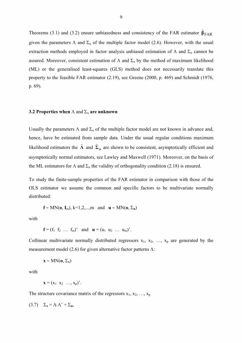
Table 3.1: Experimental design
Experimentation factor
1. Number of factors (m) One-factor model Two-factor models
2. Number of explanatory variables (p)
3, 4, 5 5, 6, 7
3. Degree of multicollinearity Moderate Strong High
4. Regression coefficients Identical Different
The Monte Carlo simulation is stratified fourfold (Table 3.1). The first experimentation factor
refers to the number of common factors, m, used to generate the regressors of the multiple
regression model (2.3). Specifically, we study one- and two-factor models with a varying
number of manifest variables, p. In the one-factor model the number of variables varies from
three to five, in the two-factor model from five to seven. The second experimentation factor p
is bounded downwards by the condition of non-negative degrees of freedom condition in the
goodness-of-fit test. The third experimentation factor captures the degree of multicollinearity.
Three degrees are distinguished: moderate, strong and high multicollinearity. Moderate
multicollinearity reflects the situation where the factor pattern of the common factors implies
correlations between 0.7 and 0.9 for respective groups of variables. Correlations between 0.90
and 0.96 within groups of variables refer define a strong degree of multicollinearity. In case of
high multicollinearity the correlations within groups of variables are larger than 0.96. Extreme
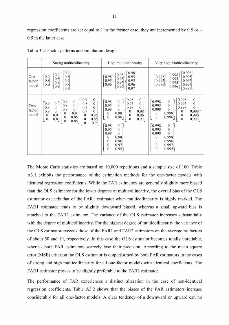
situations of virtually perfect multicollinearity are not covered. Table 3.2 exhibits the special
factor patterns studied by Monte Carlo methods.3 The fourth experimentation factor refers to
the choice of identical or different components of the coefficient vector β. While all
3 The simulations are carried out with MATLAB Version 6.5.
11
regression coefficients are set equal to 1 in the former case, they are incremented by 0.5 or –
0.5 in the latter case.
Table 3.2: Factor patterns and simulation design
Strong multicollinearity High multicollinearity Very high Multicollinearity
One-factor model
9.08.09.08.09.0
;8.09.08.09.0
;9.08.09.0
97.096.095.095.098.0
;96.095.095.098.0
;96.095.098.0
997.0996.0995.0995.0998.0
;996.0995.0995.0998.0
;996.0995.0998.0
Two-factor model
9.0085.0085.0009.009.008.009.0
;
85.0085.009.00
09.008.009.0
;
8.009.00
09.008.009.0
;
97.0096.0098.00098.0095.0098.0
;
96.0098.00098.0095.0098.0
95.0097.0096.0098.00098.0095.0098.0
;
997.00996.00998.000998.00995.00998.0
;
996.00998.000998.00995.00998.0
995.00997.00996.00998.000998.00995.00998.0
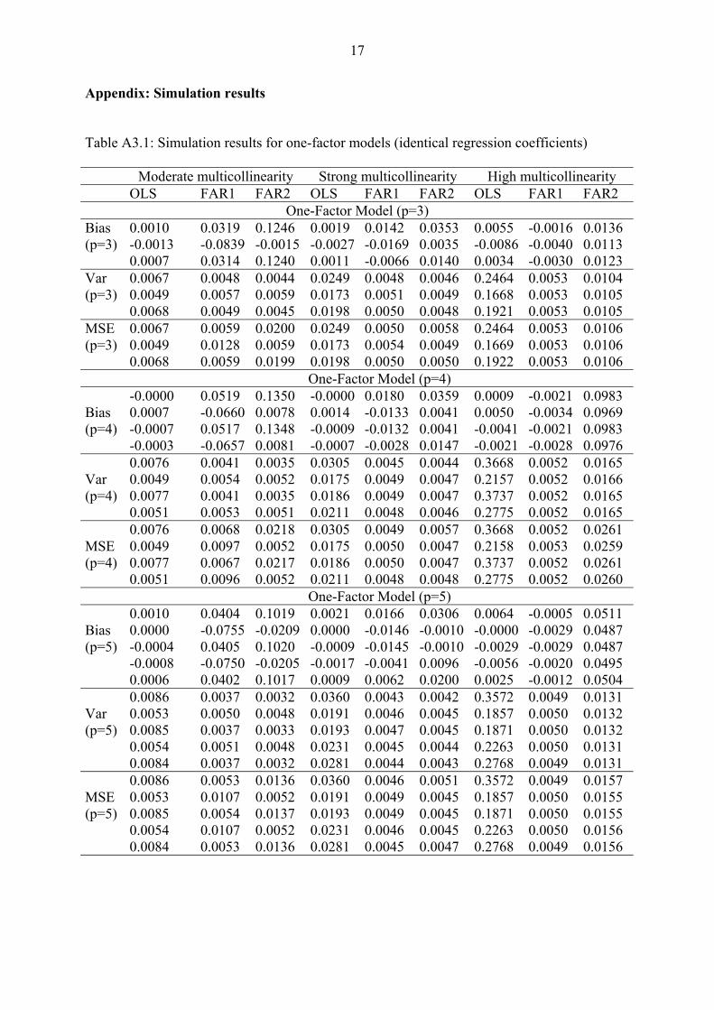
The Monte Carlo statistics are based on 10,000 repetitions and a sample size of 100. Table
A3.1 exhibits the performance of the estimation methods for the one-factor models with
identical regression coefficients. While the FAR estimators are generally slightly more biased
than the OLS estimator for the lower degrees of multicollinearity, the overall bias of the OLS
estimator exceeds that of the FAR1 estimator when multicollinearity is highly marked. The
FAR1 estimator tends to be slightly downward biased, whereas a small upward bias is
attached to the FAR2 estimator. The variance of the OLS estimator increases substantially
with the degree of multicollinearity. For the highest degree of multicollinearity the variance of
the OLS estimator exceeds those of the FAR1 and FAR2 estimators on the average by factors
of about 50 and 19, respectively. In this case the OLS estimator becomes totally unreliable,
whereas both FAR estimators scarcely lose their precision. According to the mean square
error (MSE) criterion the OLS estimator is outperformed by both FAR estimators in the cases
of strong and high multicollinearity for all one-factor models with identical coefficients. The
FAR1 estimator proves to be slightly preferable to the FAR2 estimator.
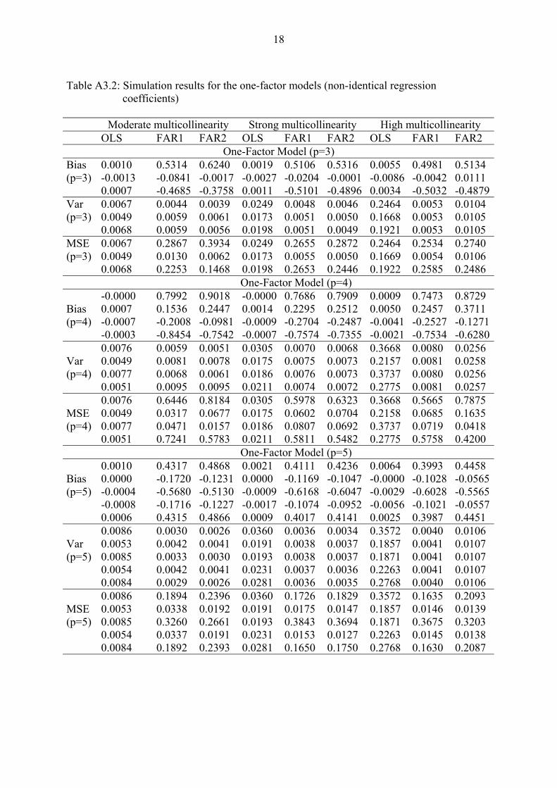
The performance of FAR experiences a distinct alteration in the case of non-identical
regression coefficients. Table A3.2 shows that the biases of the FAR estimators increase
considerably for all one-factor models. A clear tendency of a downward or upward can no
12
more be stated. However, a tendency of FAR estimation to equalize the effects of the
explanatory variables on the dependent variable becomes obvious. With it the high precision
of the FAR estimators is still retained. The average variance inflation factors (46 and 18)
coming along with OLS estimation do not alter noticeable compared with the case of identical
coefficients. Although OLS always ranks first in both lower degrees multicollinearity, its
performance deteriorates in the factor analysis regression models which are subjugated to
high multicollinearity. Only in the regression model with four explanatory variables the bias
of the FAR estimators turns out to be more severe than the loss of precision by OLS
estimation. In most of the cases the Bartlett-type FAR1 estimator outperforms the Thompson-
type FAR2 estimator.
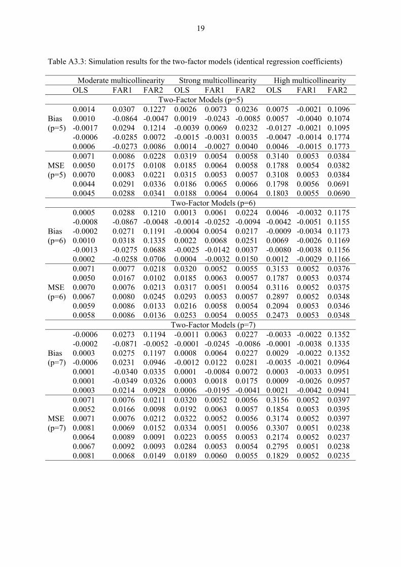
In the two-factor models with identical regression coefficients (Table A3.3) FAR estimation
proved to be preferable to OLS estimation for both higher degrees of multicollinearity. Only
in case of the lowest degree of multicollinearity the high precision of the FAR estimators
cannot fully compensate their larger downward and upward biases. Again the variance
inflation attached to the OLS estimator is much higher in relation to the FAR1 estimator as
with the FAR2 estimator. In the highest degree of multicollinearity its variance is inflated on
the average by the factors 54 and 14, respectively. Again the Bartlett-type FAR1 estimator
proves to be superior to the Thompson-type FAR2 estimator due to its smaller bias and higher
precision.
As with the one-factors models Table A3.4 exhibits a tendency of FAR estimation to
equalization in the two-factor models with non-identical regression. More specifically
estimated regression coefficients of the groups of variables generated by a common factor
seem to differ only randomly from one another. For the lowest degree of multicollinearity the
OLS estimators outperforms the FAR estimators in respect to both bias and precision. In case
of strong multicollinearity the gain in precision of both estimators cannot level out the adverse
equalization tendency. When multicollinearity is highly marked, however, the variance
inflation of the OLS estimator again turns out to be considerable. Compared with the FAR1
estimator the variance inflation factor on the average takes a value of about 25. This illustrates
once more that the FAR1 estimator clearly outperforms the FAR2 estimator with respect to
precision. Although OLS can maintain its position against the Thompson-type FAR2
estimator for the highest degree of multicollinearity it falls short against the Bartlett-type
FAR1 estimator.
13
On the whole the simulation study shows how the trade-off between bias and precision
manifests with OLS and FAR estimation. On the one hand the bias attached with OLS
estimation turns out to be negligible for typically low-dimensional factor models. Due to a
tendency of averaging of the effects of the variables related to the same common factor,
feasible FAR estimators can become considerably biased. However, they retain their high
precision under all experimental conditions, while the variance of the OLS estimator is
inflated substantially with the degree of multicollinearity. When multicollinearity is highly
marked the OLS estimator becomes totally unstable. Although specifically the Bartlett-type
feassible FAR estimator can outperform OLS under these circumstances, it only performs
satisfactorily when the influences the explanatory variables within a factor group exert on the
regressand do not differ significantly.
Thus, in case of high multicollinearity, generally neither the OLS estimator nor the FAR
estimator of 2nd type, i.e. the FAR estimator with respect to the “true” regressors ξ1, ξ2, …, ξp
will be an adequate choice. When the explanatory variables are prone to measurement errors
and multicollinearity is highly marked, the FAR estimator of 1st type, i.e. the FAR estimator
with respect to the common factors f1, f2, …, fm, gains attraction for it is not adversely
affected by both data problems. A sensible application of this kind of FAR estimator in
empirical research, however, crucially depends on the interpretability of the dimensions
underlying the explanatory variables.
4. Conclusions
When multicollinearity is highly marked OLS goes along with highly inflated variances that
can entirely invalidate statistical inference in an econometric model. Employing principal
components regression in this situation could not yet gain broad acceptance, as its
interpretation runs into difficulties (Greene, 1997, p. 427). Principal components regression
basically stands for a pure transformation method and not for an explicit modelling approach.
When the researcher intends to explicitly account for errors in variables a multiple factor
model can be used as a measurement model for the explanatory variables. Factor analysis
regression is a model-based approach to coping with multicollinearity when variables are
measured with errors.
Although factor analysis regression has been treated in several papers by different modelling
approaches, finite-sample properties of FAR estimators in the case of unknown parameters of
14
the factor model have not yet been established. In this paper this issue has been addressed by
means of Monte Carlo simulation. It turns out that unbiasedness and consistency given the
parameters of the factor model are only of limited importance when they are actually
unknown. Monte Carlo simulations uncover the particular behaviour of two feasible variants
of a theoretically attractive FAR estimator in comparison with the OLS estimator.
The simulation study reveals that the OLS estimator becomes totally unstable when
multicollinearity is highly marked. While the bias of the OLS estimator remains negligible, its
variance is substantially inflated. In contrary, both FAR estimators are expelled by a high
precision, whereas their biases cannot be ignored in all stratifications. Although more biased
the Bartlett-type feasible FAR estimator outperforms the OLS estimator in the highest grade
of multicollinearity.
Although an FAR estimator may be favourable compared with the OLS estimator when
multicollinearity is highly marked, a distinct adverse feature is unmasked from the
experimental study. FAR estimation tend to equalize the effects of the explanatory variables
on the dependent variable within a factor group. Only when the regressors within a factor
group exert identically influences on the regressand, the feasible FAR estimators solve the
problem of multicollinearity very efficiently. In case of different influences FAR estimation is
suitable to identify only the average effect of the explanatory variables loading on the same
common factor. Single effects are mixed by balancing low and high effects.
As a result both OLS and FAR do not provide satisfactory procedures to cope with high
multicollinearity. However, the problem of the division of a common factor effect on the
dependent variable in FAR does only refer to feasible estimators with respect to the
explanatory variables (FAR estimator of 2nd type). The effects of the common factors on the
dependent variable are not mixed. On this ground the employment of the FAR estimator of 1st
type can be of advantage provided that the dimensions of the set of explanatory variables are
accessible to a sensible economic interpretation.
References
Amemiya, T. (1985), Advanced Econometrics, Harvard University Press, Cambridge, Mass. Anselin, L. (1988), Spatial Econometrics: Models and Methods, Kluwer, Dordrecht.
15
Anderson, T.W. and Rubin, H. (1956), Statistical Inference in Factor Analysis, in: Proceedings of the Third Berkeley Symposium on Mathematical Statistics and Probability V, 111-150.
Basilevsky, A. (1981), Factor Analysis Regression, Canadian Journal of Statistics 9, 109-117. Basilevsky, A. (1994), Statistical Factor Analysis and Related Methods, Wiley, New York. Brachinger, W. and Ost, F. (1996), Modelle mit latenten Variablen: Faktorenanalyse, Latent-
Structure-Analyse und LISREL-Analyse, in: Fahrmeir, L., Hamerle, A. and Tutz, G. (eds.), Multivariate statistische Verfahren, 2nd ed., de Gruyter, Berlin, 639-766.
Chan, N.N. (1977), On an Unbiased Predictor in Factor Analysis, Biometrika 64, 642-644. Dillon, W.R. and Goldstein, M. (1984), Multivariate Analysis, Wiley, New York. Fahrmeir, L., Hamerle, A. and Tutz, G. (eds.) (1996), Multivariate statistische Verfahren, 2nd
ed., de Gruyter, Berlin. Fomby, T.B., Hill, R.C. and Johnson, S.R. (1984), Advanced Econometric Methods, Springer,
New York. Greene, W.H. (2000, 2003), Econometric Analysis, 4th and 5th ed., Prentice Hall, London. Isogawa, Y. and Okamato, M. (1980), Linear Prediction in the Factro Analysis Model,
Biometrika 67, 482-484. Judge, G.G., Hill, R.C., Griffiths, W.E., Lütkepohl, H. and Lee, T.-C. (1988), Introduction to
the Theory and Practice of Econometrics, 2nd ed., Wiley, New York. Jöreskog, K.G. (1977), Factor Analysis by Least Squares and Maximum Likelihood, in:
Enslein, K., Ralston, A. and Wilf, H.F. (eds.), Statistical Methods for Digital Computers, Wiley, New York, 125-153.
Johnson, R.A. and Wichern, D.W. (1992), Applied Multivariate Analysis, Prentice-Hall,
London. Johnston, J. and DiNardo, J. (1997), Econometric Methods, 4th ed., McGraw-Hill, New York. King, B. (1969), Comment on “Factor Analysis and Regression”, Econometrica 37, 538-540. Lawley, D.N. and Maxwell, A.E. (1971), Factor Analysis as a Statistical Method,
Butterworth, London. Lawley, D.N. and Maxwell, A.E. (1973), Regression and Factor Analysis, Biometrika 60,
331-338. Mardia, K.V., Kent, J.T. and Bibby, J.M. (1979), Multivariate Analysis, Academic Press,
London.

16
McDonald, R.P. and Burr, E.J. (1967), A Comparison of Four Methods of Constructing Factor Scores, Psychometrika 32, 381-401.
Schmidt, P. (1976), Econometrics, Dekker, New York. Scott, J.T. (1966), Factor Analysis and Regression, Econometrica 34, 552-562. Scott, J.T. (1969), Factor Analysis and Regression Revisited, Econometrica 37, 719. Thurstone, L.L. (1970), Multiple Factor Analysis. A Development and Expansion of “The
Vectors of Mind”, 8th ed., 1969, University of Chicago Press, Chicago.
17
Appendix: Simulation results Table A3.1: Simulation results for one-factor models (identical regression coefficients) Moderate multicollinearity Strong multicollinearity High multicollinearity OLS FAR1 FAR2 OLS FAR1 FAR2 OLS FAR1 FAR2
One-Factor Model (p=3) Bias 0.0010 0.0319 0.1246 0.0019 0.0142 0.0353 0.0055 -0.0016 0.0136 (p=3) -0.0013 -0.0839 -0.0015 -0.0027 -0.0169 0.0035 -0.0086 -0.0040 0.0113 0.0007 0.0314 0.1240 0.0011 -0.0066 0.0140 0.0034 -0.0030 0.0123 Var 0.0067 0.0048 0.0044 0.0249 0.0048 0.0046 0.2464 0.0053 0.0104 (p=3) 0.0049 0.0057 0.0059 0.0173 0.0051 0.0049 0.1668 0.0053 0.0105 0.0068 0.0049 0.0045 0.0198 0.0050 0.0048 0.1921 0.0053 0.0105 MSE 0.0067 0.0059 0.0200 0.0249 0.0050 0.0058 0.2464 0.0053 0.0106 (p=3) 0.0049 0.0128 0.0059 0.0173 0.0054 0.0049 0.1669 0.0053 0.0106 0.0068 0.0059 0.0199 0.0198 0.0050 0.0050 0.1922 0.0053 0.0106 One-Factor Model (p=4) -0.0000 0.0519 0.1350 -0.0000 0.0180 0.0359 0.0009 -0.0021 0.0983 Bias 0.0007 -0.0660 0.0078 0.0014 -0.0133 0.0041 0.0050 -0.0034 0.0969 (p=4) -0.0007 0.0517 0.1348 -0.0009 -0.0132 0.0041 -0.0041 -0.0021 0.0983 -0.0003 -0.0657 0.0081 -0.0007 -0.0028 0.0147 -0.0021 -0.0028 0.0976 0.0076 0.0041 0.0035 0.0305 0.0045 0.0044 0.3668 0.0052 0.0165 Var 0.0049 0.0054 0.0052 0.0175 0.0049 0.0047 0.2157 0.0052 0.0166 (p=4) 0.0077 0.0041 0.0035 0.0186 0.0049 0.0047 0.3737 0.0052 0.0165 0.0051 0.0053 0.0051 0.0211 0.0048 0.0046 0.2775 0.0052 0.0165 0.0076 0.0068 0.0218 0.0305 0.0049 0.0057 0.3668 0.0052 0.0261 MSE 0.0049 0.0097 0.0052 0.0175 0.0050 0.0047 0.2158 0.0053 0.0259 (p=4) 0.0077 0.0067 0.0217 0.0186 0.0050 0.0047 0.3737 0.0052 0.0261 0.0051 0.0096 0.0052 0.0211 0.0048 0.0048 0.2775 0.0052 0.0260 One-Factor Model (p=5) 0.0010 0.0404 0.1019 0.0021 0.0166 0.0306 0.0064 -0.0005 0.0511 Bias 0.0000 -0.0755 -0.0209 0.0000 -0.0146 -0.0010 -0.0000 -0.0029 0.0487 (p=5) -0.0004 0.0405 0.1020 -0.0009 -0.0145 -0.0010 -0.0029 -0.0029 0.0487 -0.0008 -0.0750 -0.0205 -0.0017 -0.0041 0.0096 -0.0056 -0.0020 0.0495 0.0006 0.0402 0.1017 0.0009 0.0062 0.0200 0.0025 -0.0012 0.0504 0.0086 0.0037 0.0032 0.0360 0.0043 0.0042 0.3572 0.0049 0.0131 Var 0.0053 0.0050 0.0048 0.0191 0.0046 0.0045 0.1857 0.0050 0.0132 (p=5) 0.0085 0.0037 0.0033 0.0193 0.0047 0.0045 0.1871 0.0050 0.0132 0.0054 0.0051 0.0048 0.0231 0.0045 0.0044 0.2263 0.0050 0.0131 0.0084 0.0037 0.0032 0.0281 0.0044 0.0043 0.2768 0.0049 0.0131 0.0086 0.0053 0.0136 0.0360 0.0046 0.0051 0.3572 0.0049 0.0157 MSE 0.0053 0.0107 0.0052 0.0191 0.0049 0.0045 0.1857 0.0050 0.0155 (p=5) 0.0085 0.0054 0.0137 0.0193 0.0049 0.0045 0.1871 0.0050 0.0155 0.0054 0.0107 0.0052 0.0231 0.0046 0.0045 0.2263 0.0050 0.0156 0.0084 0.0053 0.0136 0.0281 0.0045 0.0047 0.2768 0.0049 0.0156
18
Table A3.2: Simulation results for the one-factor models (non-identical regression coefficients) Moderate multicollinearity Strong multicollinearity High multicollinearity OLS FAR1 FAR2 OLS FAR1 FAR2 OLS FAR1 FAR2
One-Factor Model (p=3) Bias 0.0010 0.5314 0.6240 0.0019 0.5106 0.5316 0.0055 0.4981 0.5134 (p=3) -0.0013 -0.0841 -0.0017 -0.0027 -0.0204 -0.0001 -0.0086 -0.0042 0.0111 0.0007 -0.4685 -0.3758 0.0011 -0.5101 -0.4896 0.0034 -0.5032 -0.4879 Var 0.0067 0.0044 0.0039 0.0249 0.0048 0.0046 0.2464 0.0053 0.0104 (p=3) 0.0049 0.0059 0.0061 0.0173 0.0051 0.0050 0.1668 0.0053 0.0105 0.0068 0.0059 0.0056 0.0198 0.0051 0.0049 0.1921 0.0053 0.0105 MSE 0.0067 0.2867 0.3934 0.0249 0.2655 0.2872 0.2464 0.2534 0.2740 (p=3) 0.0049 0.0130 0.0062 0.0173 0.0055 0.0050 0.1669 0.0054 0.0106 0.0068 0.2253 0.1468 0.0198 0.2653 0.2446 0.1922 0.2585 0.2486 One-Factor Model (p=4) -0.0000 0.7992 0.9018 -0.0000 0.7686 0.7909 0.0009 0.7473 0.8729 Bias 0.0007 0.1536 0.2447 0.0014 0.2295 0.2512 0.0050 0.2457 0.3711 (p=4) -0.0007 -0.2008 -0.0981 -0.0009 -0.2704 -0.2487 -0.0041 -0.2527 -0.1271 -0.0003 -0.8454 -0.7542 -0.0007 -0.7574 -0.7355 -0.0021 -0.7534 -0.6280 0.0076 0.0059 0.0051 0.0305 0.0070 0.0068 0.3668 0.0080 0.0256 Var 0.0049 0.0081 0.0078 0.0175 0.0075 0.0073 0.2157 0.0081 0.0258 (p=4) 0.0077 0.0068 0.0061 0.0186 0.0076 0.0073 0.3737 0.0080 0.0256 0.0051 0.0095 0.0095 0.0211 0.0074 0.0072 0.2775 0.0081 0.0257 0.0076 0.6446 0.8184 0.0305 0.5978 0.6323 0.3668 0.5665 0.7875 MSE 0.0049 0.0317 0.0677 0.0175 0.0602 0.0704 0.2158 0.0685 0.1635 (p=4) 0.0077 0.0471 0.0157 0.0186 0.0807 0.0692 0.3737 0.0719 0.0418 0.0051 0.7241 0.5783 0.0211 0.5811 0.5482 0.2775 0.5758 0.4200 One-Factor Model (p=5) 0.0010 0.4317 0.4868 0.0021 0.4111 0.4236 0.0064 0.3993 0.4458 Bias 0.0000 -0.1720 -0.1231 0.0000 -0.1169 -0.1047 -0.0000 -0.1028 -0.0565 (p=5) -0.0004 -0.5680 -0.5130 -0.0009 -0.6168 -0.6047 -0.0029 -0.6028 -0.5565 -0.0008 -0.1716 -0.1227 -0.0017 -0.1074 -0.0952 -0.0056 -0.1021 -0.0557 0.0006 0.4315 0.4866 0.0009 0.4017 0.4141 0.0025 0.3987 0.4451 0.0086 0.0030 0.0026 0.0360 0.0036 0.0034 0.3572 0.0040 0.0106 Var 0.0053 0.0042 0.0041 0.0191 0.0038 0.0037 0.1857 0.0041 0.0107 (p=5) 0.0085 0.0033 0.0030 0.0193 0.0038 0.0037 0.1871 0.0041 0.0107 0.0054 0.0042 0.0041 0.0231 0.0037 0.0036 0.2263 0.0041 0.0107 0.0084 0.0029 0.0026 0.0281 0.0036 0.0035 0.2768 0.0040 0.0106 0.0086 0.1894 0.2396 0.0360 0.1726 0.1829 0.3572 0.1635 0.2093 MSE 0.0053 0.0338 0.0192 0.0191 0.0175 0.0147 0.1857 0.0146 0.0139 (p=5) 0.0085 0.3260 0.2661 0.0193 0.3843 0.3694 0.1871 0.3675 0.3203 0.0054 0.0337 0.0191 0.0231 0.0153 0.0127 0.2263 0.0145 0.0138 0.0084 0.1892 0.2393 0.0281 0.1650 0.1750 0.2768 0.1630 0.2087
19
Table A3.3: Simulation results for the two-factor models (identical regression coefficients) Moderate multicollinearity Strong multicollinearity High multicollinearity OLS FAR1 FAR2 OLS FAR1 FAR2 OLS FAR1 FAR2
Two-Factor Models (p=5) 0.0014 0.0307 0.1227 0.0026 0.0073 0.0236 0.0075 -0.0021 0.1096 Bias 0.0010 -0.0864 -0.0047 0.0019 -0.0243 -0.0085 0.0057 -0.0040 0.1074 (p=5) -0.0017 0.0294 0.1214 -0.0039 0.0069 0.0232 -0.0127 -0.0021 0.1095 -0.0006 -0.0285 0.0072 -0.0015 -0.0031 0.0035 -0.0047 -0.0014 0.1774 0.0006 -0.0273 0.0086 0.0014 -0.0027 0.0040 0.0046 -0.0015 0.1773 0.0071 0.0086 0.0228 0.0319 0.0054 0.0058 0.3140 0.0053 0.0384 MSE 0.0050 0.0175 0.0108 0.0185 0.0064 0.0058 0.1788 0.0054 0.0382 (p=5) 0.0070 0.0083 0.0221 0.0315 0.0053 0.0057 0.3108 0.0053 0.0384 0.0044 0.0291 0.0336 0.0186 0.0065 0.0066 0.1798 0.0056 0.0691 0.0045 0.0288 0.0341 0.0188 0.0064 0.0064 0.1803 0.0055 0.0690 Two-Factor Models (p=6) 0.0005 0.0288 0.1210 0.0013 0.0061 0.0224 0.0046 -0.0032 0.1175 -0.0008 -0.0867 -0.0048 -0.0014 -0.0252 -0.0094 -0.0042 -0.0051 0.1155 Bias -0.0002 0.0271 0.1191 -0.0004 0.0054 0.0217 -0.0009 -0.0034 0.1173 (p=6) 0.0010 0.0318 0.1335 0.0022 0.0068 0.0251 0.0069 -0.0026 0.1169 -0.0013 -0.0275 0.0688 -0.0025 -0.0142 0.0037 -0.0080 -0.0038 0.1156 0.0002 -0.0258 0.0706 0.0004 -0.0032 0.0150 0.0012 -0.0029 0.1166 0.0071 0.0077 0.0218 0.0320 0.0052 0.0055 0.3153 0.0052 0.0376 0.0050 0.0167 0.0102 0.0185 0.0063 0.0057 0.1787 0.0053 0.0374 MSE 0.0070 0.0076 0.0213 0.0317 0.0051 0.0054 0.3116 0.0052 0.0375 (p=6) 0.0067 0.0080 0.0245 0.0293 0.0053 0.0057 0.2897 0.0052 0.0348 0.0059 0.0086 0.0133 0.0216 0.0058 0.0054 0.2094 0.0053 0.0346 0.0058 0.0086 0.0136 0.0253 0.0054 0.0055 0.2473 0.0053 0.0348 Two-Factor Models (p=7) -0.0006 0.0273 0.1194 -0.0011 0.0063 0.0227 -0.0033 -0.0022 0.1352 -0.0002 -0.0871 -0.0052 -0.0001 -0.0245 -0.0086 -0.0001 -0.0038 0.1335 Bias 0.0003 0.0275 0.1197 0.0008 0.0064 0.0227 0.0029 -0.0022 0.1352 (p=7) -0.0006 0.0231 0.0946 -0.0012 0.0122 0.0281 -0.0035 -0.0021 0.0964 0.0001 -0.0340 0.0335 0.0001 -0.0084 0.0072 0.0003 -0.0033 0.0951 0.0001 -0.0349 0.0326 0.0003 0.0018 0.0175 0.0009 -0.0026 0.0957 0.0003 0.0214 0.0928 0.0006 -0.0195 -0.0041 0.0021 -0.0042 0.0941 0.0071 0.0076 0.0211 0.0320 0.0052 0.0056 0.3156 0.0052 0.0397 0.0052 0.0166 0.0098 0.0192 0.0063 0.0057 0.1854 0.0053 0.0395 MSE 0.0071 0.0076 0.0212 0.0322 0.0052 0.0056 0.3174 0.0052 0.0397 (p=7) 0.0081 0.0069 0.0152 0.0334 0.0051 0.0056 0.3307 0.0051 0.0238 0.0064 0.0089 0.0091 0.0223 0.0055 0.0053 0.2174 0.0052 0.0237 0.0067 0.0092 0.0093 0.0284 0.0053 0.0054 0.2795 0.0051 0.0238 0.0081 0.0068 0.0149 0.0189 0.0060 0.0055 0.1829 0.0052 0.0235
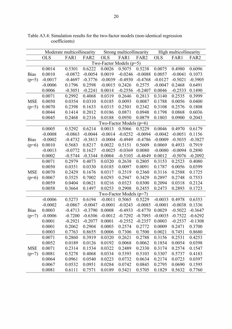
20
Table A3.4: Simulation results for the two-factor models (non-identical regression coefficients) Moderate multicollinearity Strong multicollinearity High multicollinearity OLS FAR1 FAR2 OLS FAR1 FAR2 OLS FAR1 FAR2
Two-Factor Models (p=5) 0.0014 0.5301 0.6222 0.0026 0.5075 0.5238 0.0075 0.4980 0.6096 Bias 0.0010 -0.0872 -0.0054 0.0019 -0.0246 -0.0088 0.0057 -0.0041 0.1073 (p=5) -0.0017 -0.4697 -0.3776 -0.0039 -0.4930 -0.4768 -0.0127 -0.5021 -0.3905 -0.0006 0.1796 0.2598 -0.0015 0.2426 0.2575 -0.0047 0.2468 0.6491 0.0006 -0.3051 -0.2241 0.0014 -0.2556 -0.2407 0.0046 -0.2533 0.1490 0.0071 0.2992 0.4068 0.0319 0.2646 0.2813 0.3140 0.2535 0.3999 MSE 0.0050 0.0354 0.0310 0.0185 0.0093 0.0087 0.1788 0.0056 0.0400 (p=5) 0.0070 0.2398 0.1633 0.0315 0.2501 0.2342 0.3108 0.2576 0.1808 0.0044 0.1414 0.2012 0.0186 0.0871 0.0948 0.1798 0.0868 0.6036 0.0045 0.2468 0.2316 0.0188 0.0950 0.0879 0.1803 0.0900 0.2043 Two-Factor Models (p=6) 0.0005 0.5292 0.6214 0.0013 0.5066 0.5229 0.0046 0.4970 0.6179 -0.0008 -0.0863 -0.0044 -0.0014 -0.0252 -0.0094 -0.0042 -0.0051 0.1156 Bias -0.0002 -0.4732 -0.3813 -0.0004 -0.4949 -0.4786 -0.0009 -0.5035 -0.3827 (p=6) 0.0010 0.5683 0.8217 0.0022 0.5151 0.5609 0.0069 0.4933 0.7919 -0.0013 -0.0772 0.1627 -0.0025 -0.0369 0.0080 -0.0080 -0.0094 0.2890 0.0002 -0.5744 -0.3344 0.0004 -0.5103 -0.4649 0.0012 -0.5076 -0.2092 0.0071 0.2979 0.4073 0.0320 0.2638 0.2805 0.3153 0.2523 0.4080 0.0050 0.0351 0.0330 0.0185 0.0097 0.0091 0.1787 0.0056 0.0399 MSE 0.0070 0.2429 0.1676 0.0317 0.2519 0.2360 0.3116 0.2588 0.1725 (p=6) 0.0067 0.3525 0.7002 0.0293 0.2947 0.3429 0.2897 0.2748 0.7553 0.0059 0.0404 0.0621 0.0216 0.0323 0.0300 0.2094 0.0318 0.2124 0.0058 0.3664 0.1497 0.0253 0.2908 0.2455 0.2473 0.2893 0.1723 Two-Factor Models (p=7) -0.0006 0.5273 0.6194 -0.0011 0.5065 0.5229 -0.0033 0.4978 0.6353 -0.0002 -0.0867 -0.0047 -0.0001 -0.0243 -0.0085 -0.0001 -0.0038 0.1336 Bias 0.0003 -0.4713 -0.3790 0.0008 -0.4933 -0.4770 0.0029 -0.5022 -0.3647 (p=7) -0.0006 -0.7200 -0.6306 -0.0012 -0.7292 -0.7093 -0.0035 -0.7522 -0.6292 0.0001 -0.2921 -0.2077 0.0001 -0.2552 -0.2357 0.0003 -0.2537 -0.1308 0.0001 0.2062 0.2904 0.0003 0.2574 0.2772 0.0009 0.2471 0.3700 0.0003 0.7763 0.8655 0.0006 0.7306 0.7500 0.0021 0.7451 0.8680 0.0071 0.2860 0.3919 0.0320 0.2621 0.2788 0.3156 0.2531 0.4253 0.0052 0.0189 0.0126 0.0192 0.0068 0.0062 0.1854 0.0054 0.0398 MSE 0.0071 0.2314 0.1534 0.0322 0.2489 0.2330 0.3174 0.2574 0.1547 (p=7) 0.0081 0.5278 0.4068 0.0334 0.5393 0.5103 0.3307 0.5737 0.4183 0.0064 0.0961 0.0540 0.0223 0.0732 0.0634 0.2174 0.0723 0.0397 0.0067 0.0532 0.0951 0.0284 0.0742 0.0845 0.2795 0.0690 0.1595 0.0081 0.6111 0.7571 0.0189 0.5421 0.5705 0.1829 0.5632 0.7760


![Nonparametric Regression - Homepage | ETH Zürich · 2018. 9. 13. · what unusual factor 1=(n p). It will be shown in section0.3.1that due to this factor, E[^˙2] = ˙2. 0.2.2 Assumptions](https://img.pdfslide.net/doc/110x75/6051384f518ef21de3468c21/nonparametric-regression-homepage-eth-zrich-2018-9-13-what-unusual-factor.jpg)