Embed Size (px)
Citation preview

Factorial Analysis of Variance
01:830:200:01-05 Fall 2013
Repeated-Measures ANOVA
Overview of the Factorial ANOVA
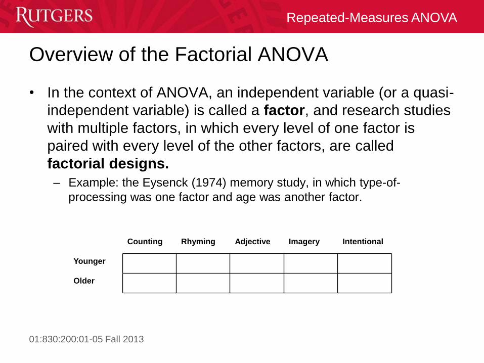
• In the context of ANOVA, an independent variable (or a quasi-
independent variable) is called a factor, and research studies
with multiple factors, in which every level of one factor is
paired with every level of the other factors, are called
factorial designs.
– Example: the Eysenck (1974) memory study, in which type-of-
processing was one factor and age was another factor.
Counting Rhyming Adjective Imagery Intentional
Younger
Older
01:830:200:01-05 Fall 2013
Repeated-Measures ANOVA
Overview of the Factorial ANOVA
• A design with m factors (with m>1) is called an m-way factorial design – The Eysenck study described in the previous slide has two factors and
is therefore a two-way factorial design
• We can design factorial ANOVAs with an arbitrary number of factors. – For example, we could add gender as another factor in the Eysenck
memory study
• However, for simplicity, we will deal only with two-way factorial designs in this course. – We will also assume that each of our factorial samples (cells) contains
the same number of scores n
01:830:200:01-05 Fall 2013
Repeated-Measures ANOVA
Overview of the Factorial ANOVA
Why might we want to use factorial designs?
• With a one-way ANOVA, we can examine the effect of
different levels of a single factor:
– E.g., How does age affect word recall?
– Or, How does type of processing affect word recall?
• We need two different experiments to determine the effects of
these two factors on memory if we use a one-way design.
• Moreover, using a factorial design allows us to detect
interactions between factors
01:830:200:01-05 Fall 2013
Repeated-Measures ANOVA
Overview of the Factorial ANOVA
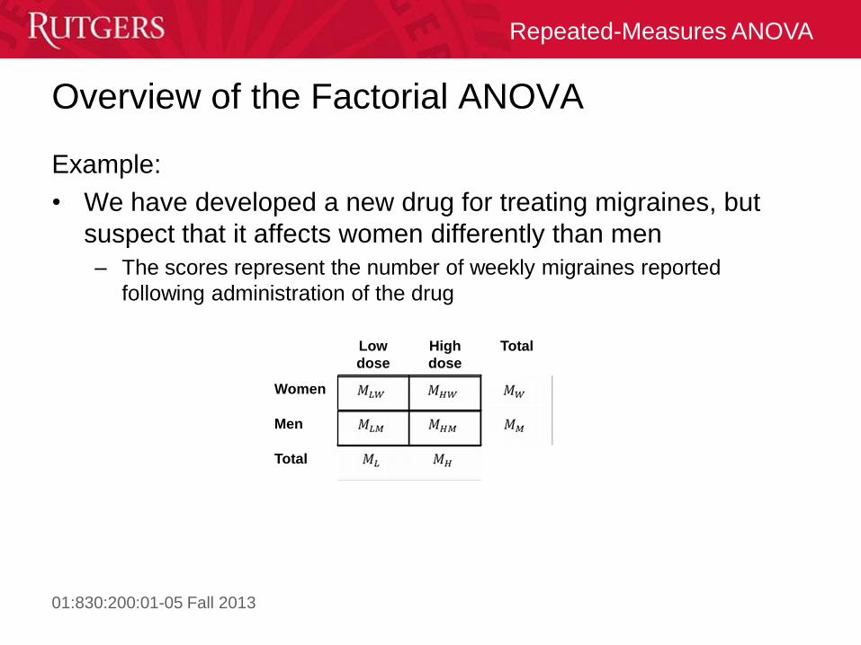
Example:
• We have developed a new drug for treating migraines, but
suspect that it affects women differently than men
– The scores represent the number of weekly migraines reported
following administration of the drug
Low
dose
High
dose
Total
Women
Men
Total

01:830:200:01-05 Fall 2013
Repeated-Measures ANOVA
Overview of the Factorial ANOVA
• Notice that the study involves two dosage conditions and two
gender conditions, creating a two-by-two matrix with a total of
4 different treatment conditions.
• Each treatment condition is represented by a cell in the
matrix.
• For an independent-measures research study (which is the
only kind of factorial design that we will consider), a separate
sample would be used for each of the four conditions.
01:830:200:01-05 Fall 2013
Repeated-Measures ANOVA
Overview of the Factorial ANOVA
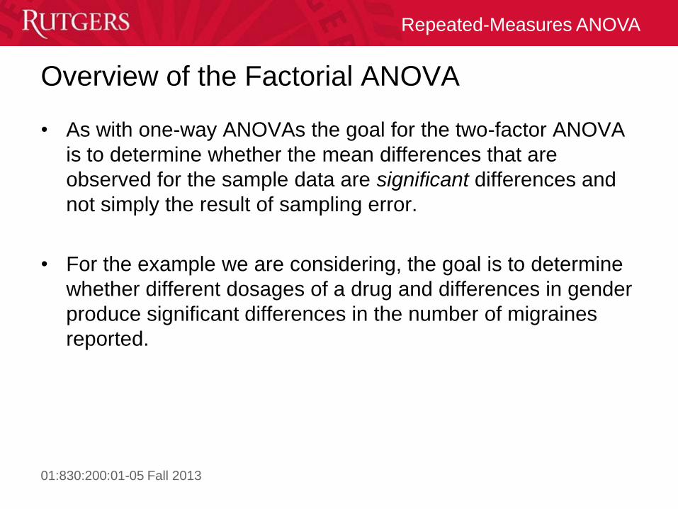
• As with one-way ANOVAs the goal for the two-factor ANOVA
is to determine whether the mean differences that are
observed for the sample data are significant differences and
not simply the result of sampling error.
• For the example we are considering, the goal is to determine
whether different dosages of a drug and differences in gender
produce significant differences in the number of migraines
reported.
01:830:200:01-05 Fall 2013
Repeated-Measures ANOVA
Factorial ANOVA Main Effects
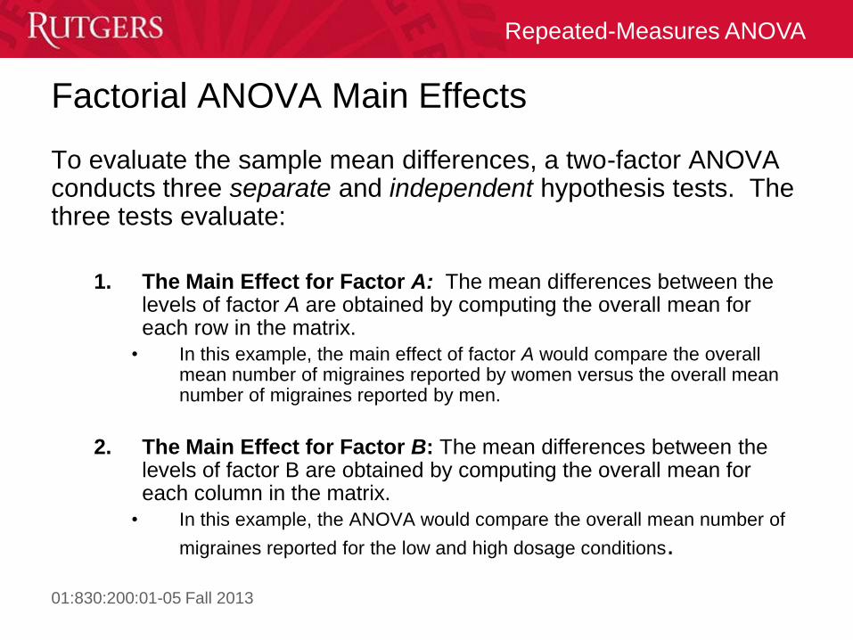
To evaluate the sample mean differences, a two-factor ANOVA conducts three separate and independent hypothesis tests. The three tests evaluate:
1. The Main Effect for Factor A: The mean differences between the
levels of factor A are obtained by computing the overall mean for each row in the matrix.
• In this example, the main effect of factor A would compare the overall mean number of migraines reported by women versus the overall mean number of migraines reported by men.
2. The Main Effect for Factor B: The mean differences between the levels of factor B are obtained by computing the overall mean for each column in the matrix.
• In this example, the ANOVA would compare the overall mean number of
migraines reported for the low and high dosage conditions.
01:830:200:01-05 Fall 2013
Repeated-Measures ANOVA
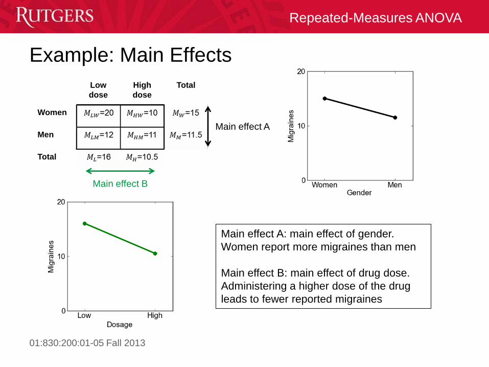
Example: Main Effects
Low
dose
High
dose
Total
Women
Men
Total
Main effect B
Main effect A
Main effect A: main effect of gender.
Women report more migraines than men
Main effect B: main effect of drug dose.
Administering a higher dose of the drug
leads to fewer reported migraines

01:830:200:01-05 Fall 2013
Repeated-Measures ANOVA
Interactions
• The A x B Interaction: Often two factors will "interact" so
that specific combinations of the two factors produce results
(mean differences) that are not explained by the overall
effects of either factor.
– For example, a particular drug may have different efficacies for men
vs. women. Different doses of the drug might produce very small
changes in men, but dramatic, or even opposite, effects in women.
This dependence on the effect of one factor (drug dosage) on another
(sex or gender) is called an interaction.

01:830:200:01-05 Fall 2013
Repeated-Measures ANOVA
Example: Interaction
Low
dose
High
dose
Total
Women
Men
Total
In this case, the drug seems to be much more effective for women than for men. We
would say that there is an interaction between the effect of gender and the effect of
drug dosage
Main effect B

01:830:200:01-05 Fall 2013
Repeated-Measures ANOVA
Example: No Interaction
Low dose High
dose
Total
Women
Men
Total
In this case, the main effect of the drug dosage is the same as in the previous case,
but there is no longer a difference between the effect of drug dosage on women
versus men. There is no interaction.
Main effect B

01:830:200:01-05 Fall 2013
Repeated-Measures ANOVA
Interactions
• This is the primary advantage of combining two factors
(independent variables) in a single research study: it allows
you to examine how the two factors interact with each other.
– That is, the results will not only show the overall main effects of each
factor, but also how unique combinations of the two variables may
produce unique results.

01:830:200:01-05 Fall 2013
Repeated-Measures ANOVA
More Examples

01:830:200:01-05 Fall 2013
Repeated-Measures ANOVA
Simple Effects
• To interpret significant interactions, researchers often conduct a fourth type of hypothesis test for simple effects
• Simple effects (or simple main effects) involve testing the effect of one factor at a particular value of the second factor – In our example, testing the effect of the drug for women only or for men only
are examples of simple effects, as are testing the effect of gender in low-dose only or high-dose only conditions
• Testing for simple effects essentially consists of running a separate one way ANOVA across all levels of one factor at a fixed level of the second factor – For example, in the Eysenck memory study, we could run a one-way
ANOVA to determine the effect of processing condition on word recall for young subjects only

01:830:200:01-05 Fall 2013
Repeated-Measures ANOVA
Example: Interaction
Low
dose
High
dose
Total
Women
Men
Total
Main effect B
01:830:200:01-05 Fall 2013
Repeated-Measures ANOVA
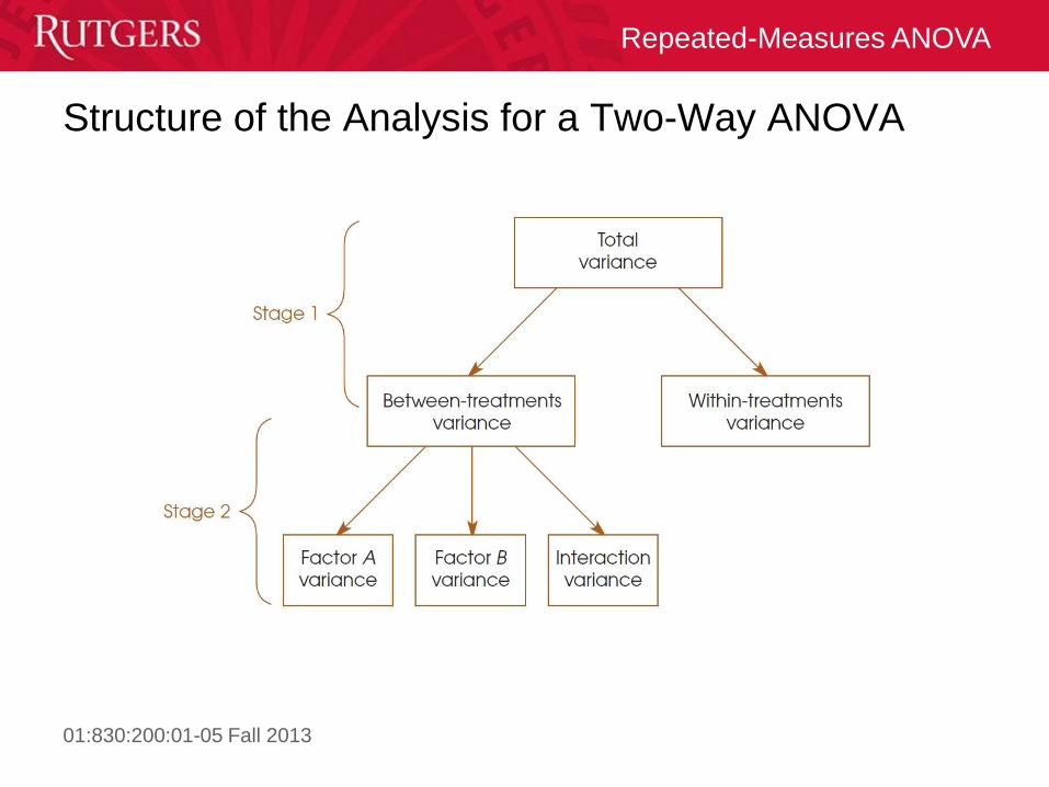
Structure of the Analysis for a Two-Way ANOVA

01:830:200:01-05 Fall 2013
Repeated-Measures ANOVA
The Two-Way ANOVA
• Each of the three hypothesis tests in a two-factor ANOVA will
have its own F-ratio and each F-ratio has the same basic
structure:
• Each MS value equals SS/df, and the individual SS and df
values are computed in a two-stage analysis.
• The first stage of the analysis is identical to the single-factor
(one-way) ANOVA and separates the total variability (SS and
df) into two basic components: between treatments and within
treatments.
between
within
MSF
MS
01:830:200:01-05 Fall 2013
Repeated-Measures ANOVA
The Two-Way ANOVA
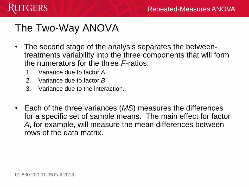
• The second stage of the analysis separates the between-treatments variability into the three components that will form the numerators for the three F-ratios: 1. Variance due to factor A
2. Variance due to factor B
3. Variance due to the interaction.
• Each of the three variances (MS) measures the differences for a specific set of sample means. The main effect for factor A, for example, will measure the mean differences between rows of the data matrix.

01:830:200:01-05 Fall 2013
Repeated-Measures ANOVA
The Two-Way ANOVA: Possible Outcomes
1. All 3 hypothesis tests are not significant
2. Only main effect of Factor A is significant
3. Only main effect of Factor B is significant
4. Both main effects (for A and B) are significant
5. Only the interaction (A×B) is significant
6. Main effect of Factor A and A×B interaction are significant
7. Main effect of Factor B and A×B interaction are significant
8. All 3 hypothesis tests are significant

01:830:200:01-05 Fall 2013
Repeated-Measures ANOVA

01:830:200:01-05 Fall 2013
Repeated-Measures ANOVA
The Two-Way ANOVA: Steps
1. State Hypotheses
2. Compute F-ratio statistic: for each main effect and their interaction
– For data in which I give you cell means and SS’s, you will have to
compute: • marginal means
• SStotal, SSbetween, SSwithin, SSfactor A, SSfactor B, & SSA×B
• dftotal, dfbetween, dfwithin, dffactor A, dffactor B, & dfA×B
3. Use F-ratio distribution table to find critical F-value(s) representing rejection region(s)
4. For each F-test, make a decision: does the F-statistic for your test fall into the rejection region?
, whateverwhatever error
error
MSF df df
MS
01:830:200:01-05 Fall 2013
Repeated-Measures ANOVA
Source df SS MS F p
Between groups
Gender
Dose
Dose x gender
Within (error)
Total
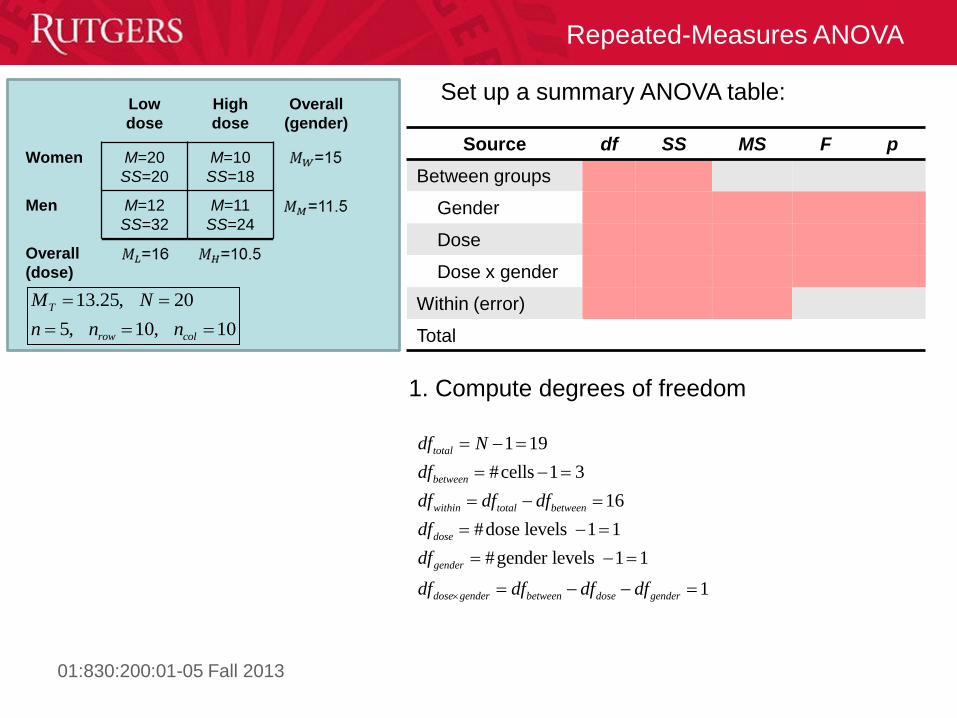
Set up a summary ANOVA table:
1. Compute degrees of freedom
Low
dose
High
dose
Overall
(gender)
Women M=20
SS=20
M=10
SS=18
Men M=12
SS=32
M=11
SS=24
Overall
(dose)
13.25, 20
5, 10, 10
T
row col
M N
n n n
cells
dose levels 1 1
gender levels
1 19
# 1 3
16
#
#
1
1 1
total
between
within total between
dose
dose gender between dose
gender
gender
df N
df
df df
df
df
df df df
d
df
f
01:830:200:01-05 Fall 2013
Repeated-Measures ANOVA
Source df SS MS F p
Between groups 3
Gender 1
Dose 1
Dose x gender 1
Within (error) 16
Total 19
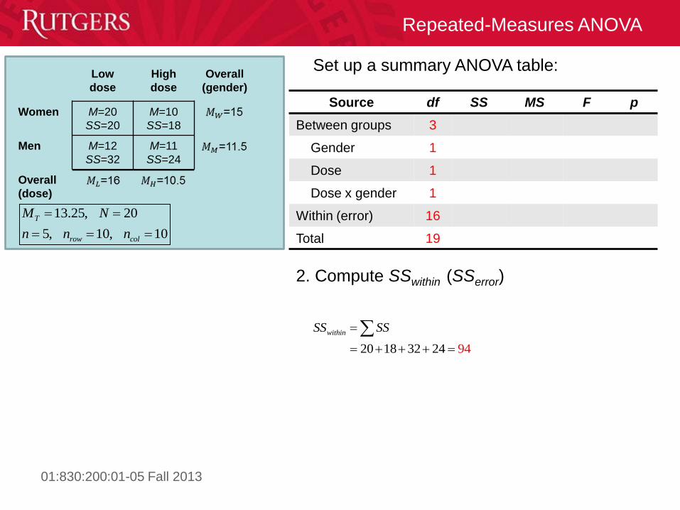
Set up a summary ANOVA table:
2. Compute SSwithin (SSerror)
20 918 32 24 4
withinSS SS
Low
dose
High
dose
Overall
(gender)
Women M=20
SS=20
M=10
SS=18
Men M=12
SS=32
M=11
SS=24
Overall
(dose)
13.25, 20
5, 10, 10
T
row col
M N
n n n

01:830:200:01-05 Fall 2013
Repeated-Measures ANOVA
Source df SS MS F p
Between groups 3
Gender 1
Dose 1
Dose x gender 1
Within (error) 16 94
Total 19
Set up a summary ANOVA table:
3. Compute SSbetween (SScells)
2
2 2 2 25 20 13.25 10 13.25 12 13.25 11 13.25
5 45.563 10.563 1.56
313
3 5.063
5 62. .7575
cell TbetweenSS n M M
Low
dose
High
dose
Overall
(gender)
Women M=20
SS=20
M=10
SS=18
Men M=12
SS=32
M=11
SS=24
Overall
(dose)
13.25, 20
5, 10, 10
T
row col
M N
n n n
01:830:200:01-05 Fall 2013
Repeated-Measures ANOVA
Source df SS MS F p
Between groups 3 313.75
Gender 1
Dose 1
Dose x gender 1
Within (error) 16 94
Total 19 407.75
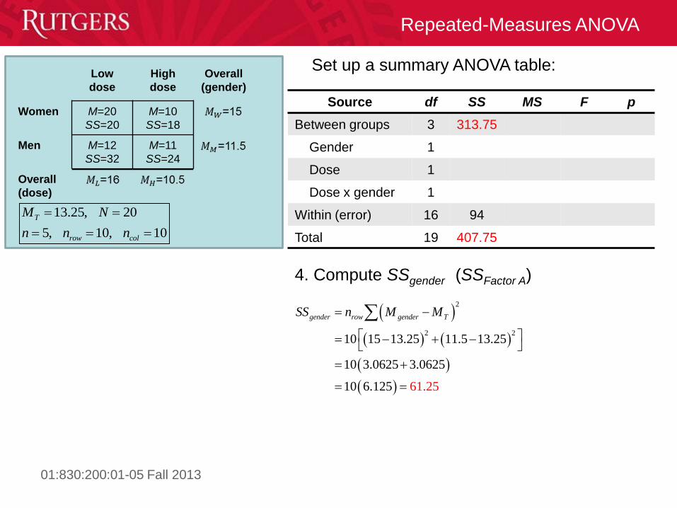
Set up a summary ANOVA table:
4. Compute SSgender (SSFactor A)
2
2 210 15 13.25 11.5 13.25
10 3.0625 3.0625
10 6. 61.25125
gender row gend r TeSS n M M
Low
dose
High
dose
Overall
(gender)
Women M=20
SS=20
M=10
SS=18
Men M=12
SS=32
M=11
SS=24
Overall
(dose)
13.25, 20
5, 10, 10
T
row col
M N
n n n

01:830:200:01-05 Fall 2013
Repeated-Measures ANOVA
Source df SS MS F p
Between groups 3 313.75
Gender 1 61.25
Dose 1
Dose x gender 1
Within (error) 16 94
Total 19 407.75
Set up a summary ANOVA table:
5. Compute SSdose (SSFactor B)
2
2 210 16 13.25 10.5 13.25
151.25
10 7.5625 7.5625
10 15.125
dose col d ToseSS n M M
Low
dose
High
dose
Overall
(gender)
Women M=20
SS=20
M=10
SS=18
Men M=12
SS=32
M=11
SS=24
Overall
(dose)
13.25, 20
5, 10, 10
T
row col
M N
n n n
01:830:200:01-05 Fall 2013
Repeated-Measures ANOVA
Source df SS MS F p
Between groups 3 313.75
Gender 1 61.25
Dose 1 151.25
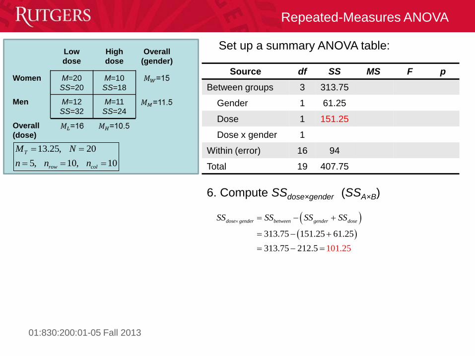
Dose x gender 1
Within (error) 16 94
Total 19 407.75
Set up a summary ANOVA table:
6. Compute SSdose×gender (SSA×B)
313.75 151.25 61.25
313.75 2 101.1 . 52 5 2
gender between gender dod seoseSS SS SS SS
Low
dose
High
dose
Overall
(gender)
Women M=20
SS=20
M=10
SS=18
Men M=12
SS=32
M=11
SS=24
Overall
(dose)
13.25, 20
5, 10, 10
T
row col
M N
n n n
01:830:200:01-05 Fall 2013
Repeated-Measures ANOVA
Source df SS MS F p
Between groups 3 313.75
Gender 1 61.25
Dose 1 151.25
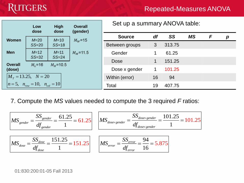
Dose x gender 1 101.25
Within (error) 16 94
Total 19 407.75
Set up a summary ANOVA table:
7. Compute the MS values needed to compute the 3 required F ratios:
661.25
11.25
gender
gender
gender
SSMS
df
95.875
4
16
errorerror
error
SSMS
df 1
151.25
151.25dose
dos
e
e
dos
SSMS
df
101101.25
1.25
dose gender
dose gender
dose gender
SSMS
df
Low
dose
High
dose
Overall
(gender)
Women M=20
SS=20
M=10
SS=18
Men M=12
SS=32
M=11
SS=24
Overall
(dose)
13.25, 20
5, 10, 10
T
row col
M N
n n n
01:830:200:01-05 Fall 2013
Repeated-Measures ANOVA
Source df SS MS F p
Between groups 3 313.75
Gender 1 61.25 61.25
Dose 1 151.25 151.25
Dose x gender 1 101.25 101.25
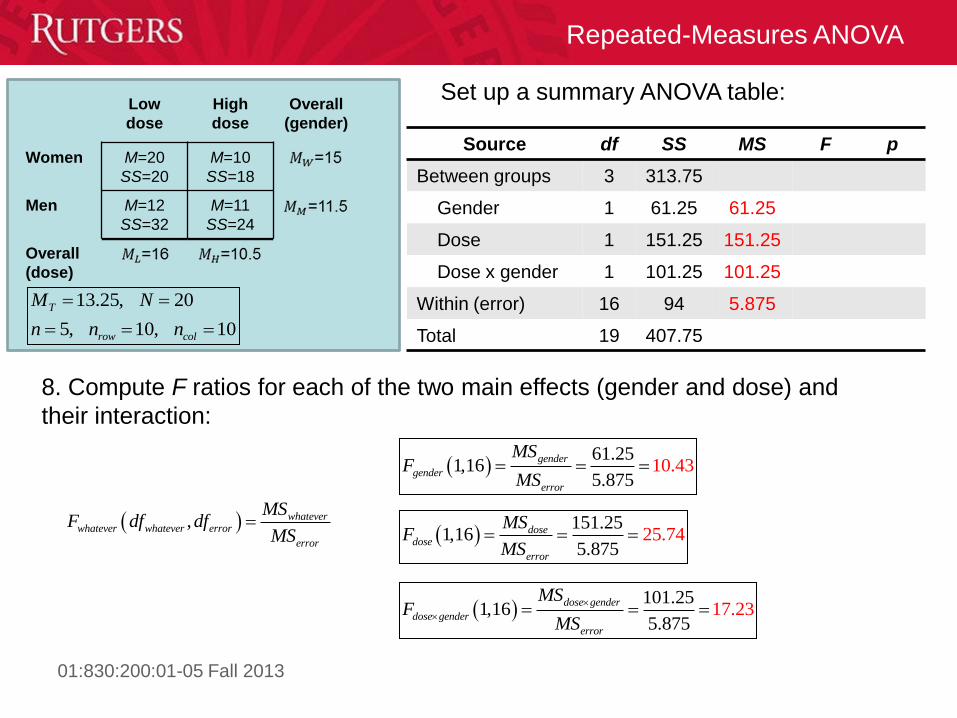
Within (error) 16 94 5.875
Total 19 407.75
Set up a summary ANOVA table:
8. Compute F ratios for each of the two main effects (gender and dose) and
their interaction:
, whateverwhatever ewhatever rror
error
dfMS
F dfMS
61.25
1,165.8
10.45
37
gender
e
ge
rro
nder
r
MSF
MS
151.25
1,165.875
25.74dose
err
e
or
dos
MSF
MS
101.25
1,1 165.
7.8
375
2genddose
dose
erro
er
g nd
r
e er
MSF
MS
Low
dose
High
dose
Overall
(gender)
Women M=20
SS=20
M=10
SS=18
Men M=12
SS=32
M=11
SS=24
Overall
(dose)
13.25, 20
5, 10, 10
T
row col
M N
n n n

01:830:200:01-05 Fall 2013
Repeated-Measures ANOVA
Source df SS MS F p
Between groups 3 313.75
Gender 1 61.25 61.25 10.43
Dose 1 151.25 151.25 25.74
Dose x gender 1 101.25 101.25 17.23
Within (error) 16 94 5.875
Total 19 407.75
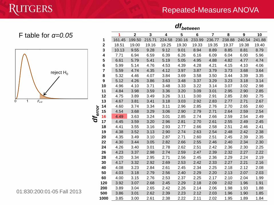
Set up a summary ANOVA table:
9. Finally, look up Fcrit for each of your obtained F values
In this case, we happen to be lucky that they all have the same degrees of
freedom (1,16), so we only have to look up one Fcrit
Low
dose
High
dose
Overall
(gender)
Women M=20
SS=20
M=10
SS=18
Men M=12
SS=32
M=11
SS=24
Overall
(dose)
13.25, 20
5, 10, 10
T
row col
M N
n n n

01:830:200:01-05 Fall 2013
Repeated-Measures ANOVA
1 2 3 4 5 6 7 8 9 10
1 161.45 199.50 215.71 224.58 230.16 233.99 236.77 238.88 240.54 241.88
2 18.51 19.00 19.16 19.25 19.30 19.33 19.35 19.37 19.38 19.40
3 10.13 9.55 9.28 9.12 9.01 8.94 8.89 8.85 8.81 8.79
4 7.71 6.94 6.59 6.39 6.26 6.16 6.09 6.04 6.00 5.96
5 6.61 5.79 5.41 5.19 5.05 4.95 4.88 4.82 4.77 4.74
6 5.99 5.14 4.76 4.53 4.39 4.28 4.21 4.15 4.10 4.06
7 5.59 4.74 4.35 4.12 3.97 3.87 3.79 3.73 3.68 3.64
8 5.32 4.46 4.07 3.84 3.69 3.58 3.50 3.44 3.39 3.35
9 5.12 4.26 3.86 3.63 3.48 3.37 3.29 3.23 3.18 3.14
10 4.96 4.10 3.71 3.48 3.33 3.22 3.14 3.07 3.02 2.98
11 4.84 3.98 3.59 3.36 3.20 3.09 3.01 2.95 2.90 2.85
12 4.75 3.89 3.49 3.26 3.11 3.00 2.91 2.85 2.80 2.75
13 4.67 3.81 3.41 3.18 3.03 2.92 2.83 2.77 2.71 2.67
14 4.60 3.74 3.34 3.11 2.96 2.85 2.76 2.70 2.65 2.60
15 4.54 3.68 3.29 3.06 2.90 2.79 2.71 2.64 2.59 2.54
16 4.49 3.63 3.24 3.01 2.85 2.74 2.66 2.59 2.54 2.49
17 4.45 3.59 3.20 2.96 2.81 2.70 2.61 2.55 2.49 2.45
18 4.41 3.55 3.16 2.93 2.77 2.66 2.58 2.51 2.46 2.41
19 4.38 3.52 3.13 2.90 2.74 2.63 2.54 2.48 2.42 2.38
20 4.35 3.49 3.10 2.87 2.71 2.60 2.51 2.45 2.39 2.35
22 4.30 3.44 3.05 2.82 2.66 2.55 2.46 2.40 2.34 2.30
24 4.26 3.40 3.01 2.78 2.62 2.51 2.42 2.36 2.30 2.25
26 4.23 3.37 2.98 2.74 2.59 2.47 2.39 2.32 2.27 2.22
28 4.20 3.34 2.95 2.71 2.56 2.45 2.36 2.29 2.24 2.19
30 4.17 3.32 2.92 2.69 2.53 2.42 2.33 2.27 2.21 2.16
40 4.08 3.23 2.84 2.61 2.45 2.34 2.25 2.18 2.12 2.08
50 4.03 3.18 2.79 2.56 2.40 2.29 2.20 2.13 2.07 2.03
60 4.00 3.15 2.76 2.53 2.37 2.25 2.17 2.10 2.04 1.99
120 3.92 3.07 2.68 2.45 2.29 2.18 2.09 2.02 1.96 1.91
200 3.89 3.04 2.65 2.42 2.26 2.14 2.06 1.98 1.93 1.88
500 3.86 3.01 2.62 2.39 2.23 2.12 2.03 1.96 1.90 1.85
1000 3.85 3.00 2.61 2.38 2.22 2.11 2.02 1.95 1.89 1.84
dfnumerator
F table for α=0.05
reject H0
df e
rro
r
01:830:200:01-05 Fall 2013
Repeated-Measures ANOVA
1 2 3 4 5 6 7 8 9 10
1 161.45 199.50 215.71 224.58 230.16 233.99 236.77 238.88 240.54 241.88
2 18.51 19.00 19.16 19.25 19.30 19.33 19.35 19.37 19.38 19.40
3 10.13 9.55 9.28 9.12 9.01 8.94 8.89 8.85 8.81 8.79
4 7.71 6.94 6.59 6.39 6.26 6.16 6.09 6.04 6.00 5.96
5 6.61 5.79 5.41 5.19 5.05 4.95 4.88 4.82 4.77 4.74
6 5.99 5.14 4.76 4.53 4.39 4.28 4.21 4.15 4.10 4.06
7 5.59 4.74 4.35 4.12 3.97 3.87 3.79 3.73 3.68 3.64
8 5.32 4.46 4.07 3.84 3.69 3.58 3.50 3.44 3.39 3.35
9 5.12 4.26 3.86 3.63 3.48 3.37 3.29 3.23 3.18 3.14
10 4.96 4.10 3.71 3.48 3.33 3.22 3.14 3.07 3.02 2.98
11 4.84 3.98 3.59 3.36 3.20 3.09 3.01 2.95 2.90 2.85
12 4.75 3.89 3.49 3.26 3.11 3.00 2.91 2.85 2.80 2.75
13 4.67 3.81 3.41 3.18 3.03 2.92 2.83 2.77 2.71 2.67
14 4.60 3.74 3.34 3.11 2.96 2.85 2.76 2.70 2.65 2.60
15 4.54 3.68 3.29 3.06 2.90 2.79 2.71 2.64 2.59 2.54
16 4.49 3.63 3.24 3.01 2.85 2.74 2.66 2.59 2.54 2.49
17 4.45 3.59 3.20 2.96 2.81 2.70 2.61 2.55 2.49 2.45
18 4.41 3.55 3.16 2.93 2.77 2.66 2.58 2.51 2.46 2.41
19 4.38 3.52 3.13 2.90 2.74 2.63 2.54 2.48 2.42 2.38
20 4.35 3.49 3.10 2.87 2.71 2.60 2.51 2.45 2.39 2.35
22 4.30 3.44 3.05 2.82 2.66 2.55 2.46 2.40 2.34 2.30
24 4.26 3.40 3.01 2.78 2.62 2.51 2.42 2.36 2.30 2.25
26 4.23 3.37 2.98 2.74 2.59 2.47 2.39 2.32 2.27 2.22
28 4.20 3.34 2.95 2.71 2.56 2.45 2.36 2.29 2.24 2.19
30 4.17 3.32 2.92 2.69 2.53 2.42 2.33 2.27 2.21 2.16
40 4.08 3.23 2.84 2.61 2.45 2.34 2.25 2.18 2.12 2.08
50 4.03 3.18 2.79 2.56 2.40 2.29 2.20 2.13 2.07 2.03
60 4.00 3.15 2.76 2.53 2.37 2.25 2.17 2.10 2.04 1.99
120 3.92 3.07 2.68 2.45 2.29 2.18 2.09 2.02 1.96 1.91
200 3.89 3.04 2.65 2.42 2.26 2.14 2.06 1.98 1.93 1.88
500 3.86 3.01 2.62 2.39 2.23 2.12 2.03 1.96 1.90 1.85
1000 3.85 3.00 2.61 2.38 2.22 2.11 2.02 1.95 1.89 1.84
dfbetween
df e
rro
r
F table for α=0.05
reject H0

01:830:200:01-05 Fall 2013
Repeated-Measures ANOVA
Source df SS MS F p
Between groups 3 313.75
Gender 1 61.25 61.25 10.43* <0.05
Dose 1 151.25 151.25 25.74* <0.05
Dose x gender 1 101.25 101.25 17.23* <0.05
Within (error) 16 94 5.875
Total 19 407.75
Set up a summary ANOVA table:
Both main effects are significant, as is their interaction. This suggests that:
1. The number of reported migraines differs between men and women • Women report more migraines than men
2. The number of reported migraines is affected by the drug • Fewer migraines are reported in the high dose condition
3. The effect of the drug differs across genders • Women are more sensitive to the drug than are men
Low
dose
High
dose
Overall
(gender)
Women M=20
SS=20
M=10
SS=18
Men M=12
SS=32
M=11
SS=24
Overall
(dose)
13.25, 20
5, 10, 10
T
row col
M N
n n n