Embed Size (px)
Citation preview
The University of Technology, Jamaica
Faculty of Engineering and Computing
School of Engineering
The Factors Impacting the Achievement of Chilled Water Set Point in an
Absorption District Cooling Plant: A Six Sigma Approach, UWI Mona Central AC Park
Major Project
In partial fulfillment of the requirement for Bachelors of Science in Industrial Engineering
June 24, 2015
Jonathan Isaacs - ID#: 0703331
Jason Bennett - ID#: 0904787
Allie Palmer - ID#: 0504654
Jhomo Marshall – ID#: 0903347
_____________________
Head of Department
_____________________
Faculty Projects Coordinator
________________________
Project Supervisor

ii
Acknowledgement
We are using this opportunity to express our gratitude to everyone who supported us
throughout the development of this project. We are thankful for their guidance, constructive
criticism and useful advice. Also we are sincerely grateful to them for sharing their truthful and
illuminating views on a number of issues related to the project. We express our warm thanks to
the plant manager and other members of the maintenance and operations team at the UWI
MONA Central AC Park. Finally, we express gratitude to our project supervisor Mr. Mark
Thomas for providing the requisite guidance and support.
iii
Table of Contents
Abstract ...................................................................................................................................................... viii
Executive Summary ..................................................................................................................................... ix
1.0 Introduction ............................................................................................................................................. 1
1.1 Brief Description ................................................................................................................................. 1
1.3 Statement of the Problem .................................................................................................................... 2
1.4 Purpose of the Study ........................................................................................................................... 2
1.5 Research Objectives ............................................................................................................................ 2
1.7 Limitations .......................................................................................................................................... 2
1.8 Delimitations ....................................................................................................................................... 3
1.9 Significance of Project ........................................................................................................................ 3
1.10 Clarification of Concepts .................................................................................................................. 4
2.0 Literature Review .................................................................................................................................... 7
2.1 Introduction ......................................................................................................................................... 7
2.2 Description and Operating Principle of Absorption District Cooling ................................................. 7
2.3 Factors Impacting Chilled Water Set Point in Absorption Cooling Systems ................................... 16
2.3.1 Cooling Tower Operation and Maintenance .............................................................................. 16
2.3.2 Faults during Operation ............................................................................................................. 18
2.3.3 Proper Chiller Maintenance ....................................................................................................... 19
2.3.4 Controls ...................................................................................................................................... 20
2.3.5 Environmental Impact on Set Point ........................................................................................... 21
2.3.6 Chiller Additives ........................................................................................................................ 21
2.4 Summary ........................................................................................................................................... 23
3.0 Methodology ......................................................................................................................................... 24
3.1 Instruments ........................................................................................................................................ 26
3.2 Executing Six Sigma Methodology ...................................................................................................... 28
3.3 Model Development .......................................................................................................................... 32
4.0 Findings................................................................................................................................................. 34
4.1 Preliminary Assessment of Process Performance ............................................................................. 34
4.2 Temperature Reading Verification .................................................................................................... 36
iv
4.3 Regression Analysis of Cooling Water Outlet Temperature, Chilled Water Outlet Temperature and
Wetbulb Temperature ............................................................................................................................. 38
4.4 Impact of Vacuuming on Chilled Water Outlet Temperature ........................................................... 42
4.5 Chiller Additives ................................................................................................................................... 43
4.6 Cooling Tower Maintenance and Operations ................................................................................... 43
4.6.1 Cooling Tower Effectiveness ..................................................................................................... 43
4.6.2 Cooling Tower Water Quality .................................................................................................... 45
4.6.4 Improvement in Chilled Water Outlet Temperature Post belt Tensioning ................................ 47
4.6.4 Number of Cooling Tower Fan Belts Verification .................................................................... 48
4.6.5 Failure Mode Effect Analysis (FMEA)...................................................................................... 50
4.7 Faults during Operation .................................................................................................................... 52
5.0 Conclusions ........................................................................................................................................... 54
6 Recommendations .................................................................................................................................... 57
References ................................................................................................................................................... 59
6.0 Appendices ............................................................................................................................................ 63
Appendix A ............................................................................................................................................. 63
Appendix B ............................................................................................................................................. 67
Appendix C ............................................................................................................................................. 70
Appendix D ............................................................................................................................................. 73
Appendix E ............................................................................................................................................. 79
Appendix F.............................................................................................................................................. 82
Appendix G ............................................................................................................................................. 83
Appendix H ............................................................................................................................................. 84
Appendix I .............................................................................................................................................. 85
Appendix J .............................................................................................................................................. 87
Appendix K ............................................................................................................................................. 88
Appendix N ............................................................................................................................................. 90
Appendix O ............................................................................................................................................. 91
Appendix P.............................................................................................................................................. 92
v
List of Figures
Figure 1 - District cooling system (Euroheat& Power, 2006) ........................................................ 8
Figure 2 - Schematic Diagram of the Absorption Chiller (Thermatec) .......................................... 9
Figure 3 - Double effect chiller system (New Building Institute 1998, p.4) ................................ 10
Figure 4 – Induced Draft Cooling Tower System (Chemical Oil Toolbox) ................................. 13
Figure 5 - Low Temperature Heat Exchanger (www.wikidot.com) ............................................. 12
Figure 6 - Vapour Absorption Refrigeration System (Singh, 2014) ............................................. 14
Figure 7 - Six Sigma Methodology (George et al, 2005) ............................................................. 24
Figure 8 - Mixed Method Design of Research (Fishcheler, 2014) ............................................... 26
Table 1. Research Variables ......................................................................................................... 28
Figure 9 –Project Timeline Phase One ......................................................................................... 30
Figure 10 – Project Timeline Phase Two ...................................................................................... 31
Figure 11: Model Design and calibration ..................................................................................... 32
Table 2. Model Calibration Results .............................................................................................. 33
Figure 12 - Process Capability Report for Chiller #1 Sep 2013 - Sep 2014 ................................ 35
Figure 13 - Process Capability Report for Chiller #2 Sep 2013 - Sep 2014 ................................ 35
Table 3. Results of Temperature Verification............................................................................... 36
Figure 14- Regression for Chilled Water vs Cooling Water Using Actual Plant Values ............. 40
Figure 15 –- Regression for Actual Cooling Water vs Actual Wetbulb Temperature .................. 41
Figure 16 –Impact of Vacuuming on Chilled Water Temperature ............................................... 42
Figure 17 . Cooling Tower Effectiveness .................................................................................... 44
Table 4- Results of Water Tests .................................................................................................... 45
Figure 18 –Improvement in Chilled Water Post belt Tensioning ................................................. 47
vi
Figure 19 –Pareto Chart of Chiller of Plant System Faults .......................................................... 52
Figure A1 - X-bar and R Chart for chiller #1 performance from Sep 2013 – Sep 2014 .............. 63
Figure A2 - X-bar and R Chart for chiller #2 performance from Sep 2013 – Sep 2014 .............. 64
Figure A3 - Chiller #1 Set point chart for Sep 2013 ..................................................................... 65
Figure A4 - Chiller #1 Set point chart for Sep 2014 ..................................................................... 66
Figure A5 - Chiller set point chart for Sep 2013 .......................................................................... 66
Figure A6 - Chiller set point chart for Sep 2014 .......................................................................... 66
Figure B1-Temperature Verification of Chilled Water Outlet Temperatures .............................. 67
Figure B2-Temperature Verification of Cooling Water Outlet Temperatures ............................. 68
Figure B3-Temperature Verification of High Temperature Generator Temperatures .................. 69
Figure C1-Results of Water Hardness Tests ................................................................................. 70
Figure C2-Results of Water pH Tests ........................................................................................... 71
Figure C3-Results of Water Totally Dissolved Solids Test .......................................................... 72
Figure D1 – Regression for Simulated Cooling Water vs Simulated Chilled Water Temperature
....................................................................................................................................................... 73
Figure D2 – Regression for Simulated Cooling Water vs Simulated Wetbulb Temperature ....... 74
Figure E2-Chiller Number One Condenser Scale Indicator ......................................................... 79
Figure E3-Chiller Number One Condenser Scale Indicator ......................................................... 80
Figure E4- Illustrating Scale Build up in Cooling Towers ........................................................... 81
Figure F1 –Improvement in Cooling Water Post Belt Tensioning ............................................... 82
Table G1- Impact of Vacuuming .................................................................................................. 83
Figure H1 –Cooling Tower Belt Failure Mode and Effect Analysis (FEMEA) ........................... 84
Figure I1 –Rapid Side Wall Wear of Cooling Tower Belts .......................................................... 85
vii
Figure I2 -Plastic Deformation of cooling Tower Belts ............................................................... 86
Figure J1 - Block diagram of Plant Layout ................................................................................... 87
Figure K1 - Daily Operational Log Sheet ..................................................................................... 88
Figure K2 - Ultrameter used at the plant to measure water parameters ........................................ 89
Figure K3 - Infrared thermometer used to verify operating temperature .................................... 89
Figure 25 – Aerial view of the UWI MONA Central AC Park and ETS ..................................... 90
Figure O1- Quarterly LiBr Sample Report ................................................................................... 91
Figure P1 - Table showing Cooling Water Quality Best Practices ............................................... 92
Figure P2- Table showing Makeup requirements at Various Cycle ............................................. 92
viii
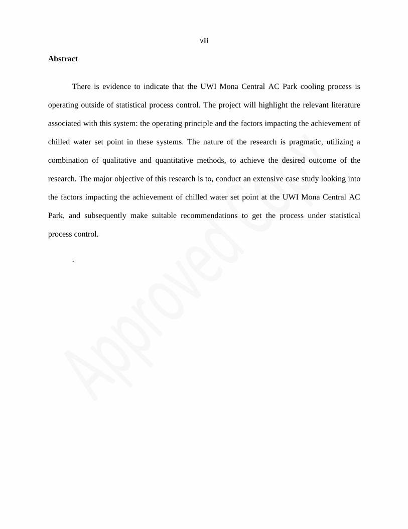
Abstract
There is evidence to indicate that the UWI Mona Central AC Park cooling process is
operating outside of statistical process control. The project will highlight the relevant literature
associated with this system: the operating principle and the factors impacting the achievement of
chilled water set point in these systems. The nature of the research is pragmatic, utilizing a
combination of qualitative and quantitative methods, to achieve the desired outcome of the
research. The major objective of this research is to, conduct an extensive case study looking into
the factors impacting the achievement of chilled water set point at the UWI Mona Central AC
Park, and subsequently make suitable recommendations to get the process under statistical
process control.
.
ix
Executive Summary
The objective of this research project is to conduct an extensive case study into the
factors impacting the achievement of chilled water set point in an absorption cooling system and,
to identify possible ways of improving the attainment of chilled water set point. Six Sigma was
selected as the methodology which best captured a systematic approach to support the case study
being executed. Combinations of both qualitative and quantitative data were collected from
several on-site visits at the facility, followed by technical evaluation and researched literature for
comparisons. Thereafter suitable recommendations were made. The following six sigma steps
were conducted to prepare the case study; Define, Measurement, Analysis of data, Improve, and
Control, (DMAIC).
Process capability assessments conducted revealed that both chillers in the plant were
below the minimum Cpk value of one. Chillers one and two had Cpk values of -0.12 and 0
respectively indicating that the process is incapable of consistently hitting the target.
Temperature verification exercises conducted on the three major system sensors indicated that
they were fully functional and within the acceptable margin of error, of 10%. Several regression
models were done seeking to highlight the relationships between cooling water inlet, chilled
water outlet, and wet bulb temperatures. A regression model comparing actual plant records and
predicted data from the plant conceptual model was done. The regression for cooling water inlet
temperature and wet bulb temperature deviated from theory, where a very strong relationship
was expected; however other factors contributed to this. Additionally, the predicted values from
the plant model simulation produced greater relationships for all three parameters being
compared again indicating other factors at work. Water Quality Parameters of conductivity,
hardness and pH fell outside of the minimum threshold standard for both the Original Equipment
x
Manufacturer (OEM) and industry standards. Total Dissolved Solids (TDS) values were within
acceptable range. The investigation revealed that important instruments such as tension meter
and laser alignment tools were missing from belt maintenance activities. This compromised the
validity of maintenance activities. Frequent belt failure negativ
temperatures and improvement in chilled water outlet temperature post belt
maintenance. Six faults accounted for 80% of disruptions in cooling on the plant: power cut,
burner fault, chilled water flow switch, freezing, cooling tower belt failure, and cooling water
flow switch. f
I k j f j ,
f
f
f k f q
f R z ff f f
f ,
- f
1
1.0 Introduction
1.1 Brief Description
Moss (2011) in a Jamaican Gleaner article, stated that Jamaica utilizes approximately 65
percent of its energy for cooling and refrigeration. According to Euro Heat & Power (2012), the
application of absorption district cooling technologies is heavily utilized in developed countries
such as Europe, as sustainable and efficient energy solutions. Due to the high cost of electricity
in the Caribbean region (World watch Institute, 2013), the rising importance of implementing
such systems is being realized.
Here in Jamaica, the UWI Mona campus is one such facility which utilizes this
technology for space cooling. The results of an energy audit at the UWI Mona Campus, carried
out by Caribbean ESCo Limited, revealed that 46% of estimated electricity end use was
consumed by air condition systems (Energy Conservation Project Office, UWI Mona, 2010).
This coupled with expansion and constructions of new facilities, has created an escalation in
electricity demand. As a result, this had prompted the proposition of a District cooling facility
(Energy Conservation Project Office, UWI Mona, n.d).
The UWI Mona Central AC Park is a crucial facility, providing space cooling for several
buildings within the district-cooling network. The buildings cooled by this plant are: Sutherland
Global Services Call Center, a section of the Mona School of Business, and the Basic Medical
Sciences Building (BMSC). Appendices J and N show the layout of UWI Mona district cooling
network. The required cooling of these buildings is particularly critical as deviations from
requirement will result in negative implications to the operations and activities within these
buildings. There are several factors which may affect the optimal performance of the system.
2
1.3 Statement of the Problem
j f UWI M A P k’
consistently maintain set point (7 +/- 1°C) as outlined by contractual agreement.
1.4 Purpose of the Study
The purpose of the study is to identify key factors impacting the achievement of chilled
water set point in absorption the district cooling plant.
1.5 Research Objectives
1. To investigate the factors impacting the achievement of chilled water set point at the
UWI Mona A.C. Park.
2. To compare factors found to the best practices for the operation of absorption district
cooling plants.
3. Make suitable recommendations to bring the process under statistical control
1.7 Limitations
There are several limitations associated with this project they include: time constraints,
plant accessibility, access to relevant literature, confidentiality and the inability to implement
recommendations.
Time Constraints
Due to the fact that there were major project deadlines that needed to be met, efforts were
primarily focused on ensuring that these deadlines were met on time. This in turn introduced
time constraints, which affected the depth and comprehensiveness of the project and the
methodologies utilized.
3
Plant Accessibility
Special arrangements had to be made with plant personnel to accommodate investigations
and data collection.
Access to Relevant Literature
Literature on absorption district cooling was limited to sources in North America, Europe
and Asia.
Confidentiality
Confidential information relating to costs and other delicate procedures were not
disclosed. In addition, as highlighted in the scope, the customer or market element will not be
explored in depth in this research. This is primarily due to the sensitive nature of operations and
activities within these buildings.
Inability to Implement Recommendations
This is a major limitation associated with the project since the implementation of
recommendations solely lies with the technical operator of the plant.
1.8 Delimitations
The research was limited to the production component of a district cooling system. This
was a direct limitation imposed on the research project.
1.9 Significance of Project
The study is significant because no studies were found on district cooling in Jamaica;
especially on absorption cooling systems. This study can create an opportunity for the technical
4
operators of the plant to develop a standardized program based on the findings and
recommendations. It can aid other technical operators of such plants and other engineering
practitioners in effecting proper maintenance and operational activities. Finally, this will add to
the existing body of knowledge on district cooling and absorption systems
1.10 Clarification of Concepts
Cooling tower Effectiveness – The United Nations Environment Programme (2006) defined
cooling tower effectiveness as the ratio between the range and the ideal range (in percentage), the
higher this ratio, the higher the cooling tower effectiveness.
Set point - According to Achterbergh and Vriens (2010) set point is defined as the desired or
target value for an essential variable of a system, often used to describe a standard configuration
or norm for the system.
Chilled Water – Skagstasd and Mildenstein (2002) defined chilled water as the commodity
typically generated at the district cooling plant by compressor driven chillers, absorption chillers
k “f ” from deep
lakes, rivers, aquifers or oceans.
Conductivity - The United Sates Environment Protection Agency (2012) defined conductivity as
a measure of the ability of water to pass an electrical current. Conductivity in water is affected
by the presence of inorganic dissolved solids such as chloride, nitrate, sulfate, and phosphate
anions (ions that carry a negative charge) or sodium, magnesium, calcium, iron, and aluminum
cautions (ions that carry a positive charge).
5
Failure modes and effects analysis (FMEA)- Mohamed Ben-Daya et al (2009)defined this as a
step-by-step approach for identifying all possible failures in a design, a manufacturing or
assembly process, or a product or service.
pH- Clugston and Flemming (2000) defined this as a measure of the acidity or alkalinity of a
solution.
Regression analysis - Allen (2007) stated that this is a statistical process for estimating the
relationships among variables. It includes many techniques for modeling and analyzing several
variables, when the focus is on the relationship between a dependent variable and one or more
independent variables.
Plant –A plant is defined as a combination of machinery, materials, money, equipment and
manpower for the ultimate goal of manufacturing a product or service.
Cooling Capacity –Maytal and Pfotenhauer (2012) highlighted cooling capacity as the rate at
which heat is removed from a refrigerated space.
Test of Null Hypothesis (p-value) – Black (2011) defined this as the smallest significance level
at which the null hypothesis would be rejected.
Total Dissolved Solids (TDS) - Palanna (2009) stated that this is the total amount of particles
dissolved in the water; it includes total amount of mobile charged ions, including minerals, salts
or metals dissolved in a given volume of water, expressed in units of mg per unit volume of
water (mg/L), also referred to as parts per million (ppm).
Delta–T (∆T) – Whitman (2009) speaks to Delta–T as the temperature difference between the
incoming water temperature and the outgoing water temperature in a chilled water system.

6
Reliability – Evans & Lindsay (2005) defined this as the probability that a product, piece of
equipment, or a system performs its intended function for a stated period of time under specified
operating conditions ().
Availability – Tont et al. (2008) defined this as the ability of system or component to perform its
required function at the stated instant or over a stated period of time.
Energy Transfer Station (ETS) -Skagstasd and Mildenstein (2002), defined the ETS as the
customer installations which provides the interface between the district cooling system and the
building cooling system.
7
2.0 Literature Review
2.1 Introduction
The literature review examined district cooling absorption systems, by looking at three
main areas: a description of the operating principle of absorption district cooling plants, the
factors impacting chilled water set point in such systems. In addition some best practices and
guidelines were highlighted on how such systems are operated
2.2 Description and Operating Principle of Absorption District Cooling
2.2.1 District Cooling
Euroheat & Power (2006) regarded the operating principle of the district cooling system
as a system in which chilled water is distributed in pipes from a central cooling plant to buildings
for space cooling and process cooling. The document identified that a district cooling system has
three major elements: the cooling source (production), a distribution system and customer
installations, Energy Transfer Station.
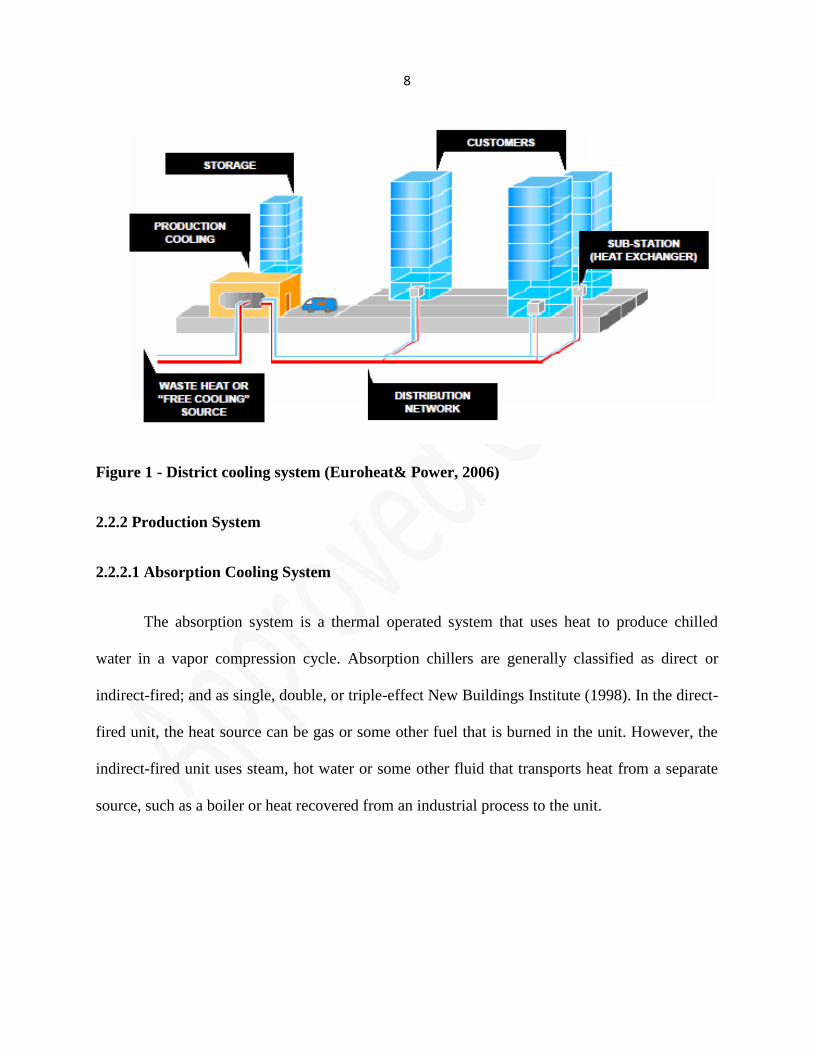
8
Figure 1 - District cooling system (Euroheat& Power, 2006)
2.2.2 Production System
2.2.2.1 Absorption Cooling System
The absorption system is a thermal operated system that uses heat to produce chilled
water in a vapor compression cycle. Absorption chillers are generally classified as direct or
indirect-fired; and as single, double, or triple-effect New Buildings Institute (1998). In the direct-
fired unit, the heat source can be gas or some other fuel that is burned in the unit. However, the
indirect-fired unit uses steam, hot water or some other fluid that transports heat from a separate
source, such as a boiler or heat recovered from an industrial process to the unit.
9
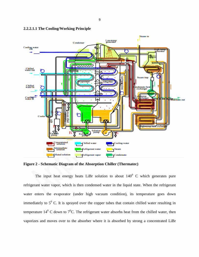
2.2.2.1.1 The Cooling/Working Principle
Figure 2 - Schematic Diagram of the Absorption Chiller (Thermatec)
The input heat energy heats LiBr solution to about 1400 C which generates pure
refrigerant water vapor, which is then condensed water in the liquid state. When the refrigerant
water enters the evaporator (under high vacuum condition), its temperature goes down
immediately to 50 C. It is sprayed over the copper tubes that contain chilled water resulting in
temperature 140 C down to 7
0C. The refrigerant water absorbs heat from the chilled water, then
vaporizes and moves over to the absorber where it is absorbed by strong a concentrated LiBr
10
solution before being pumped to the generator(s). The cooling water takes away the heat and
ejects it into the atmosphere via the cooling tower.
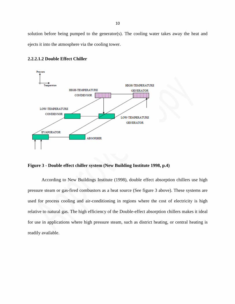
2.2.2.1.2 Double Effect Chiller
Figure 3 - Double effect chiller system (New Building Institute 1998, p.4)
According to New Buildings Institute (1998), double effect absorption chillers use high
pressure steam or gas-fired combustors as a heat source (See figure 3 above). These systems are
used for process cooling and air-conditioning in regions where the cost of electricity is high
relative to natural gas. The high efficiency of the Double-effect absorption chillers makes it ideal
for use in applications where high pressure steam, such as district heating, or central heating is
readily available.
11
2.2.2.1.3 Sub components of Absorption Cooling Systems
2.2.2.1.3.1 Evaporator
Whitman et al. (2009) highlighted that the evaporator is responsible for absorbing heat
from the necessary medium to be cooled. The heat-absorbing process is done by maintaining the
evaporator coil at a lower temperature and pressure than the medium to be cooled. The
evaporator vaporizes the refrigerant water to create a heat exchange with the incoming chilled
water. The optimum working pressure of the evaporator is 6.5mmHg.
2.2.2.1.3.2 Generator
In the generator, the diluted solution LiBr is heated by means of steam, hot water or
direct (gas/oil) firing. The diluted solution releases the refrigerant vapor (water), thus becoming
concentrated. The hot concentrated solution now regains its affinity strength and absorbs more
refrigerant then returns to the absorber. A heat exchanger is used to preheat the cold LiBr
solution before its get to the generator, (Bahtia 2012). The two common application of generators
in these systems are: high temperature generator (HTG) and the low temperature generator
(LTG) Workin f H G f : ≈ 00 H ,
≈ ° W k f L G: ≈ H ,
≈ 0°
2.2.2.1.3.3 High Temperature Heat Exchanger
Heat is recovered from the intermediate solution in the High Temperature Generator, improving
the thermodynamic coefficient of the absorption chiller system
12
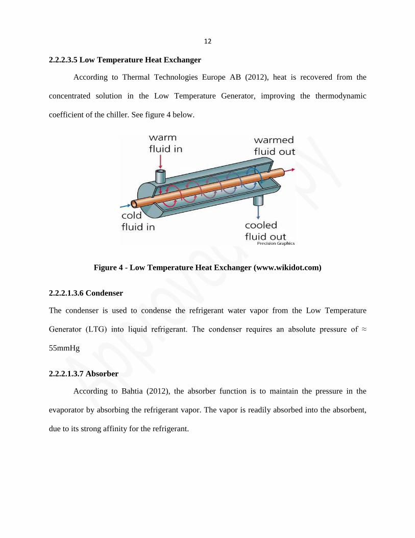
2.2.2.3.5 Low Temperature Heat Exchanger
According to Thermal Technologies Europe AB (2012), heat is recovered from the
concentrated solution in the Low Temperature Generator, improving the thermodynamic
coefficient of the chiller. See figure 4 below.
Figure 4 - Low Temperature Heat Exchanger (www.wikidot.com)
2.2.2.1.3.6 Condenser
The condenser is used to condense the refrigerant water vapor from the Low Temperature
G L G q f q f ≈
55mmHg
2.2.2.1.3.7 Absorber
According to Bahtia (2012), the absorber function is to maintain the pressure in the
evaporator by absorbing the refrigerant vapor. The vapor is readily absorbed into the absorbent,
due to its strong affinity for the refrigerant.
13
2.2.2.1.4 Cooling Tower
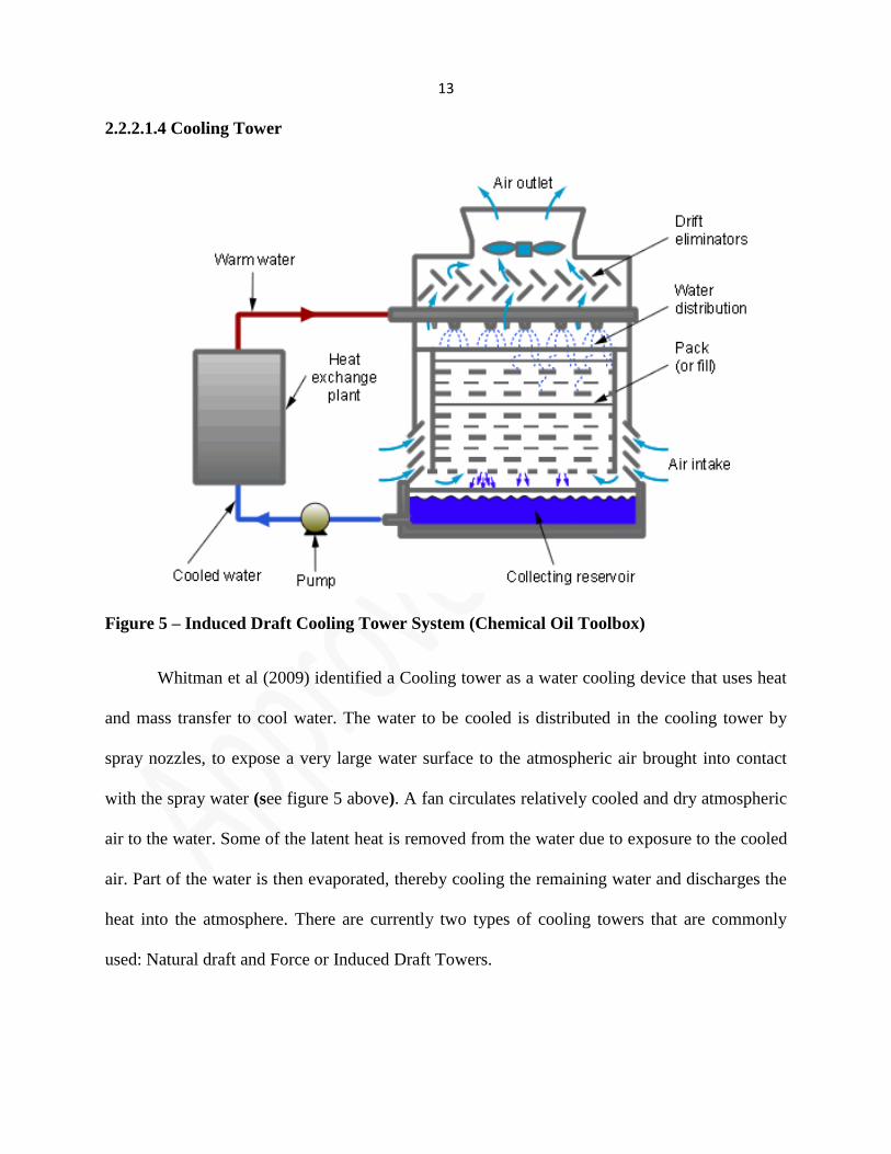
Figure 5 – Induced Draft Cooling Tower System (Chemical Oil Toolbox)
Whitman et al (2009) identified a Cooling tower as a water cooling device that uses heat
and mass transfer to cool water. The water to be cooled is distributed in the cooling tower by
spray nozzles, to expose a very large water surface to the atmospheric air brought into contact
with the spray water (see figure 5 above). A fan circulates relatively cooled and dry atmospheric
air to the water. Some of the latent heat is removed from the water due to exposure to the cooled
air. Part of the water is then evaporated, thereby cooling the remaining water and discharges the
heat into the atmosphere. There are currently two types of cooling towers that are commonly
used: Natural draft and Force or Induced Draft Towers.
14
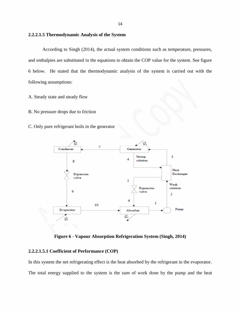
2.2.2.1.5 Thermodynamic Analysis of the System
According to Singh (2014), the actual system conditions such as temperature, pressures,
and enthalpies are substituted in the equations to obtain the COP value for the system. See figure
6 below. He stated that the thermodynamic analysis of the system is carried out with the
following assumptions:
A. Steady state and steady flow
B. No pressure drops due to friction
C. Only pure refrigerant boils in the generator
Figure 6 - Vapour Absorption Refrigeration System (Singh, 2014)
2.2.2.1.5.1 Coefficient of Performance (COP)
In this system the net refrigerating effect is the heat absorbed by the refrigerant in the evaporator.
The total energy supplied to the system is the sum of work done by the pump and the heat
15
supplied in the generator. Therefore, the (COP) of the system is given by COP =
COP =Qe/(Qg+Wp).
Neglecting the Pump work, COP = Qe/Qgis the expression for Coefficient of Performance (COP)
of the System, (Singh 2014).
2.2.2.2 Distribution
Stagstad and Mildenstein (2002), described how water is distributed from the cooling
plant to the customers through supply pipes and returned. The article further explained the
method of how pumps distributed the chilled water by creating a pressure differential (DP)
between the supply and the return lines.
District cooling systems typically vary the chilled water supply temperature based on the
ambient temperature. Seasonal heat gains/losses in buried chilled water distribution systems are
very small. Stagstad and Mildenstein (2002) stated that the chilled water temperature needs to be
supplied at a sufficiently low temperature to achieve the desired dehumidification of the supply
air, even at lower outside ambient dry bulb temperature conditions.
2.2.2.3 ETS
The Energy Transfer Station (ETS) consists of isolation and control valves, controllers,
measurement instruments, energy meter and crossover bridge, that is the hydraulic de-coupler
and or heat exchangers. The ETS should be designed for direct or indirect connection to the
district cooling distribution system. With direct connection, the district cooling water is
distributed within the building directly to terminal equipment such as air handling and fan coil
16
units, induction units, etc. An indirect connection utilizes one or multiple heat exchangers
between the district system and the building system.
2.3 Factors Impacting Chilled Water Set Point in Absorption Cooling Systems
2.3.1 Cooling Tower Operation and Maintenance
U.S. Department of Energy (2014) indicated that a cooling tower regulates temperature
by dissipating heat from re-circulating water to cool chillers, air conditioning equipment, and
other process equipment. Since heat is rejected form the tower primarily through evaporation, a
cooling tower consumes a significant amount of water.
The thermal efficiency and longevity of a cooling tower depends on the proper
management of water re-circulated through the tower. Water leaves a cooling tower system in
any one of four ways:
1. Evaporation
This is the method used to transfer heat to the environment through the vaporization of
water in the cooling tower.
2. Drift
A small quantity of water may be carried from the tower as mist or small droplets. Drift
loss is small compared to evaporation and blow down, and is controlled by baffles and drift
eliminators.
3. Blow down/Bleed Off
When water evaporates from the tower, dissolved solids such as calcium, magnesium,
chloride and silica are left behind. As more water evaporates, the concentration of dissolved
17
solids increases. If the concentration gets too high, the solids can cause scale to form within the
system or the dissolved solids can lead to a corrosion problem. The concentration of dissolved
scolds is controlled by blow down. Carefully monitoring and controlling the quantity of blow
down provides the most significant opportunity to conserve water in operations.
4. Basin Leaks/Over Flow
Properly operated cooling towers should not have leaks or overflow. Float control
equipment should be checked to ensure the basin level is being maintained properly and system
valves also checked to make sure there are no uncounted losses.
2.3.1.1 Cooling Tower Monitoring and Treatment
Bhaita (2012) stated that the treatment of cooling tower water is an important factor for
the chiller. If the water quality is not good the heat transfer tubes may form a scale on the interior
surfaces and become corroded. The heat transfer capability will decrease, causing changes in
chilled water temperature and a waste of the driving source energy.
U.S. Department of Energy (2014), recomended the installation of a conductivity
controller to continuously measure the conductivity of the cooling tower water and automatically
blow down, discharging water only when the conductivity set point is exceeded. For further
monitoring, flow meters should also be installed on makeup and blow down lines. To supplement
these monitoring devices, the ratio of makeup flow to blow down flow must be checked, along
with the ratio of conductivity of blow down and makeup water. A hand held conductivity meter
can be used if the tower is not equipped with permanent meters. These ratios should match the
target cycles of concentration. System components must be checked and if both ratios are not
about the same, check the tower for leaks or other unauthorized draw off. A key parameter used
18
to evaluate cooling tower operation is the cycle of concentration. If the tower fails to maintain
the target cycle of concentration, check system components including conductivity controller,
makeup water fill valve and blow down valve (see table 4). In order to quickly identify problems,
the conductivity and flow meters must be read regularly. Keep a log of blow down quantities;
conductivity and cycle of concentration also monitor trends to spot deterioration in performance.
2.3.2 Faults during Operation
2.3.2.1 Crystallization
Whitman et al. (2009) stated that the use of salt solution for absorption cooling creates
the possibility of the solution becoming too concentrated and actually turn back to rock salt. This
may occur if the chiller is operated under the wrong conditions. If the cooling tower water is
allowed to become too cold while operating at full load, the condenser will become too efficient
and remove too much water from the concentrate. This will result in a strong solution that has
too little water. When this solution passes through the heat exchanger, it will turn to crystals and
restrict the flow of the solution. If this is not corrected a complete blockage will occur and the
chiller will stop cooling. There are various methods to prevent this condition. One such method
is to drop the pressure in the heat exchanger by opening a valve between the refrigerant circuit
and the absorber fluid circuit to make the wear solution very weak for long enough to relieve the
problem. When the situation is corrected the valve is closed and the system resumes normal
operations. Another method is to shut down the chiller for a dilution cycle when over
concentration occurs.
19
2.3.3 Proper Chiller Maintenance
2.3.3.1 Vacuum Management
According to Bhatia (2012), the evaporator should ideally be maintained under vacuum
of approximately 6.5mmHg, this enables the refrigerant water to boil at approximately 5°C. Yin
(2006) cited that if air leaks into the chiller or if corrosion occurs this can lead to the generation
of non-condensable gases in the evaporator and absorber, which will significantly reduce the rate
of heat and mass, transfer, hence the overall cooling capacity of the chiller. An appropriate
means of removing non-condensable gases is essential to the operation of absorption chillers.
The vacuum can be maintained through an automatic gas purge device (AGPD) and/or by
periodic manual vacuum removal of non-condensable gases from the absorber and the evaporator
to maintain the required vacuum. Non-condensable gases are also generated in the HTG and the
LTG; however it is hard to remove through an AGPD. Therefore, manual vacuum removal is still
required to purge the non-condensable gases from the storage chamber and the upper vessel
(HTG and the LTG).
Piper (1999), stated that maintenance is important and critical for proper operation of
absorption chillers. If the chiller is not properly maintained this will results in reliability and
availability issues. Two particular maintenance concerns are maintaining the proper vacuum
condition in the evaporator and absorber and controlling corrosion in the chiller. Stanford III
(2011), stated that absorption chillers have three significant maintenance elements; Mechanical
Component, Heat Transfer Component and Controls.
20
2.3.3.2 Mechanical Components
Absorption chillers have refrigerant and solution pump, a purge unit and a burner that
must be maintained. The pumps are hermetically sealed, cooled and lubricated by the refrigerant
and must be annually inspected. On a daily basis the operation of the purge unit must be checked
for both proper and excess operation, indicating an air leak. This can result in air corrosion,
contamination of the absorbent solution and reduction in the efficiency and capacity. Basic
burner maintenance entails: Inspection and stack/breeching repair, cleaning of heating surfaces,
checking of combustion air intakes, testing of all safety controls, testing of relief or safety valve
for operation and set point, conducting efficiency tests and finally adjusting air/fuel ration at
least twice per year.
2.3.3.3 Heat Transfer Components
The condenser and absorber heat exchanger tubes must be cleaned annually. Lithium
Bromide solution must be analyzed annually for contamination, pH, corrosion-inhibitor level and
performance additives. Leak testing using the pressure method is required annually. Eddy current
testing of the absorber, condenser, generator and evaporator should be done every three to five
years. Absorption chillers have a number of service valves, which contain rubber diaphragm
which should be replaced every three years.
2.3.4 Controls
Proper operation of controls is critical to prevent problems with absorption chillers. Clean
and tighten all connections including field sensor connections, also vacuum control cabinets to
remove dirt and dust.
21
2.3.5 Environmental Impact on Set Point
2.3.5.1 Wet Bulb Temperature
Rockwell & Lee (2012) defined wet bulb temperature as an indication of the amount of
moisture contained in the air. The larger the differential between dry bulb and wet bulb
temperature is the dryer the air feels. Wet bulb temperature can be used to determine other
physical properties of air such as the relative humidity and the dew point temperature. One
means of determining the physical properties of air is by charting the known values on a
psychometric chart and by interpolating the other values.
The wet bulb temperature is the lowest temperature that can be supplied by a cooling tower or an
evaporative cooler. Thermal Technologies Europe AB (2012) stated that the range temperature is
the difference between the cooling tower water supply and the cooling tower water return
temperature. Y.A. Li, M.Z. Yu and G.L. Xu, (2001) cited wet bulb temperature as the primary
parameter that affects the performance of cooling towers and thus has a negative effect on the
performance of a chiller. Through this relationship it is evident that cooling capacity and the
energy consumed by a chiller are reduced by a reduction in the ambient wet bulb temperature.
2.3.6 Chiller Additives
Kaushik (2014) stated that "the cycle efficiency and operation characteristics of an
absorption cooling system depend on the properties of refrigerant, absorbent and their mixtures."
Chiller additives are added to the chiller's working fluid to improve the most important thermo-
physical properties. These include: heat of vaporization of refrigerant, heat of solution, vapor
pressure of refrigerant and absorbent, solubility of refrigerant in solvent, heat capacity of
solution, viscosity of solution and surface tension and thermal conductivity of the solution. They
22
are also used to influence the working fluid's toxicity, chemical stability and corrosivity.
Manipulation of these parameters allows for an improvement in absorber efficiency. Tomforde
(2012), categorized additives used in such systems as surfactants. These include 2-Ethyl-Hexanol
or n-Octanol and nanoparticles as Fe particles or carbon nanotubes (CNT). Others include
corrosion inhibitors such as Lithium Chromate (Li2CrO4) and Lithium Molybdate (Li2MO2) and
extra salts (ZnBr and ZnCl2) may also be added.
2.3.6.1 Surfactants
Tomforde & Luke (2012), identified octanol as an example of a surfactant, when added it
reduces the surface tension, and increases the combining capacity of solution and water vapor
will be hence the absorption efficiency will be increased. It also serves to increase the
condensation capacity of the condenser. When octanol is added, the copper tubes will soak the
water vapor creating a layer of film that will improve heat transfer efficiency.
2.3.6.2 Corrosion inhibitors
Herold, Radermacher, & Sanford (1996), highlighted that "in the presence of dissolved
oxygen LiBr is highly aggressive to many metals including carbon steel and cupper." Herold et
al, further elaborated that the inside of a chiller provides a hermetic environment which then
results in slower corrosion rates, but over the life of the machine significant corrosion can still
occur. The corrosion of iron or copper in the presence of an electrolyte such as aqueous LiBr is a
multistep oxidation- reduction reaction, involving Fe or Cu ions leaving the solid surface and
combing with oxygen:
Iron: Fe + H2O + ½ H2O + ¼ O2 Fe(OH)2
Fe(OH)2 + ½ H2O + ¼ O2 Fe(OH)3
23
4 Fe(OH)2 Fe3O4 + Fe + 4 H2O
Copper: 2Cu + ¼ O2 Cu2O
Cu2O + ½ O2 + 2 H2O Cu(OH)2
Thus corrosion inhibitors are used to minimize these effects. They reduce corrosion by reacting
with surface and forming a relative stable oxide coating, as shown above.
Lithium Chromate (Li2CrO4):
3 Fe + 6 H2O + 2 Li2CrO4 Fe3O4 + 2 Cr(OH)3 + 4 LiOH + H2
3 Fe + 6 H2O + 2 Li2CrO4 Fe3O4 + 2 Cr3O3 + LiOH + H2
6 Cu + 5 H2O + 2 Li2CrO4 3Cu2O + Cr(OH)3 + 4 LiOH
Lithium Molybdate (Li2MoO2):
3 Fe + 6 H2O + Li2MoO4 FeO4 + MoO2 + 2 LiOH + 3H2
2 Cu + H2O + Li2MoO4 Cu2O + MoO2 + 2 LiOH
2.3.6.3 Extra Salts
Extra Salts LiBr as a working fluid in high concentration is prone to crystallization. The
addition of extra salts such as ZnBr and ZnCl2 pushes the normal operating zone. As a result a
string solution can be cooled in the crystallization, which improves the performance of the
system, (Kaushik & Singh, 2014).
2.4 Summary
The literature review discussed the absorption district cooling system, looking at two key
areas: description and operating principle of absorption district cooling plants, and the factors
impacting the achievement of chilled water set point in such systems.
24
3.0 Methodology
The focus of this research was on the production system of the UWI Mona Central AC
Park where the factors impacting the achievement of chilled water set point were analyzed and
highlighted by conducting an extensive case study. Balbach (1999) cited a case study as a useful
evaluation tool when implementing an existing program in a new setting. Swanborn (2010),
highlighted that in carrying out an extensive case study information is collected about a large
number of instances of a phenomenon, conclusions are then drawn by putting together all the
information and finally calculating and interpreting correlations between the properties of these
instances. An extensive case study was the ideal approach as it provided the best strategy to
study the wide range of variables, which affected the process and their interrelation.
Six Sigma was chosen as the ideal methodology to carry out this research, because its
structure encouraged creative thinking within the boundaries of the process. According to Evans
and Lindsey (2010), it is a business improvement approach that seeks to find and eliminate
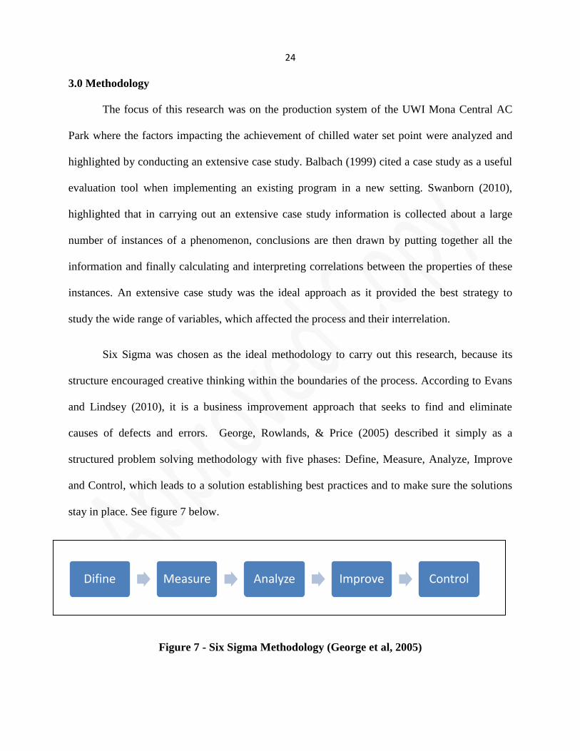
causes of defects and errors. George, Rowlands, & Price (2005) described it simply as a
structured problem solving methodology with five phases: Define, Measure, Analyze, Improve
and Control, which leads to a solution establishing best practices and to make sure the solutions
stay in place. See figure 7 below.
Figure 7 - Six Sigma Methodology (George et al, 2005)
Difine Measure Analyze Improve Control
25
After a Six Sigma project is selected, Evans and Lindsey (2010) along with George, Rowlands,
& Price (2005) listed the following steps for carrying out a Six Sigma study:
Definition - Once the project was identified, the first step was to clearly define the problem and
validate the scope of the project.
Measurement -This was done to understand the current state of the process and develop
operational definitions for all performance measures.
Analysis of the data - This was done to verify key variables that were most likely to create
errors and excessive variation. Data charts and other analysis were done to determine the
correlation between these variables and the critical output of the system.
Improve - Once the root cause of the problem was understood, corrective actions for resolving
the problem were established.
Control - This is done to establish procedures to maintain the gains attained by the improvement
stage.
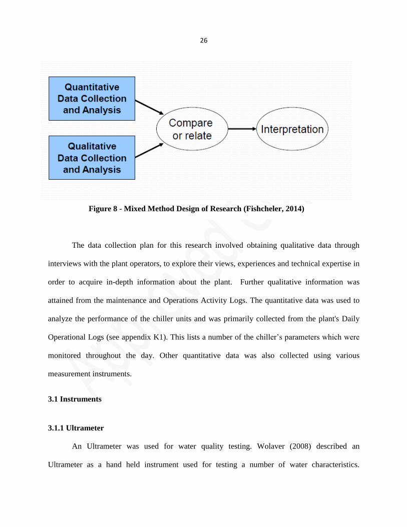
Klenke (2008) outlined that pragmatism supports the use of both qualitative and quantitative
methods in the same study, because the complexity of the research demands multiple methods
(See Figure 8). A mixed method approach is applied to this research as it has been recognized
that one method does not provide all the information required. This variation in data collection
leads to greater validity of research results and answers questions from a number of perspectives.
26
The data collection plan for this research involved obtaining qualitative data through
interviews with the plant operators, to explore their views, experiences and technical expertise in
order to acquire in-depth information about the plant. Further qualitative information was
attained from the maintenance and Operations Activity Logs. The quantitative data was used to
analyze the performance of the chiller units and was primarily collected from the plant's Daily
Operational Logs (see appendix K1). This lists a number of the ’
monitored throughout the day. Other quantitative data was also collected using various
measurement instruments.
3.1 Instruments
3.1.1 Ultrameter
An Ultrameter was used for water quality testing. Wolaver (2008) described an
Ultrameter as a hand held instrument used for testing a number of water characteristics.
Figure 8 - Mixed Method Design of Research (Fishcheler, 2014)
27
According to Myrron L Company (2013) it has the ability to perform in-cell conductometric
titrations that provides a convenient way to determine alkalinity and hardness. The model
delivers performance of ±1% of reading and a four-digit LCD shares measurement values up to
9999 (see appendix K2).
3.1.2 Infrared thermometer
An infrared thermometer was used for taking and confirming sensor temperature
readings. Kirkham (2004) stated that this device has the ability to measure temperature from a
distance. This allowed the measurement of temperature especially in applications where
conventional methods could not be employed (see appendix K3).
3.1.3 Dial stem thermometer
Lipta (2003) stated that a dial stem thermometer uses a bimetal spring as a temperature
sensing element. This technology uses a coil spring made of two different types of metals that
are welded or fastened together. These metals can be copper, steel or brass as long as one has
low heat sensitivity and the other metal has high heat sensitivity. Whenever the welded strip is
heated, the two metals change length based on their individual rates of thermal expansion. The
movement of the strip is to deflect a pointer over a calibrated scale which then indicates
temperature to the user. The accuracy of this thermometer according to Thermco Products Inc.
(2014) is +/- 1% over the entire scale. This particular type of thermometer was chosen because of
its accuracy and the ability to insert it in direct contact with the fluids in the water loops.
28
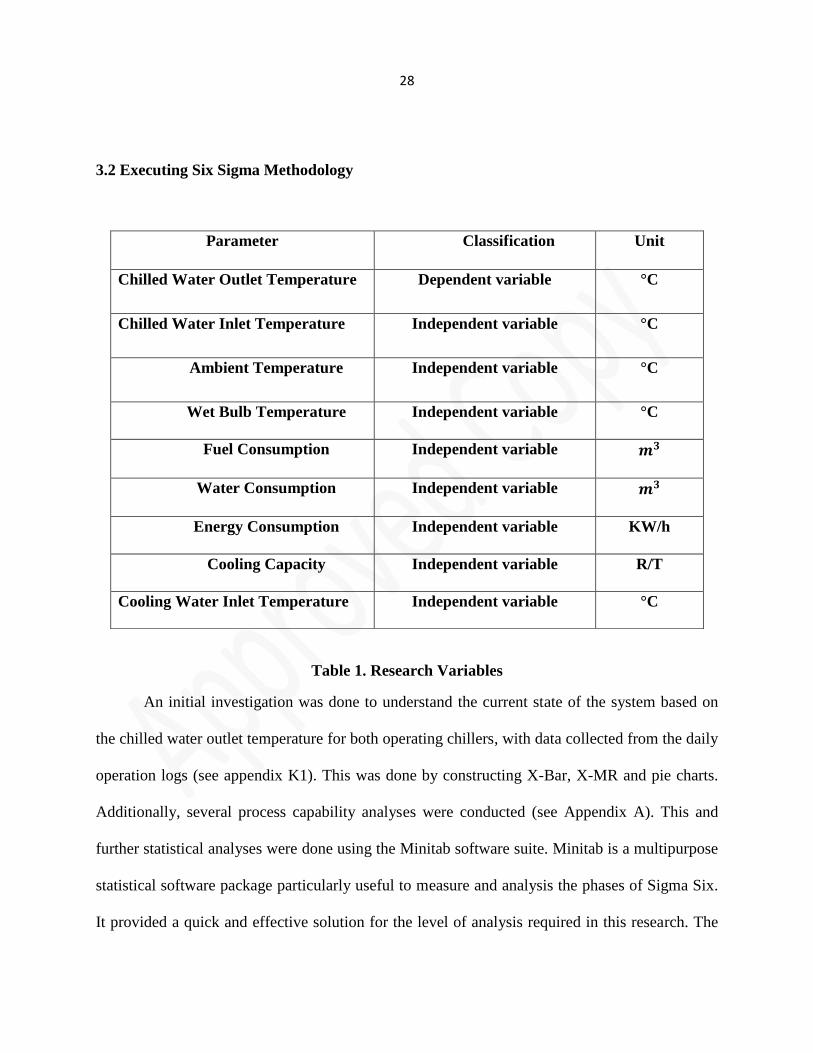
3.2 Executing Six Sigma Methodology
Table 1. Research Variables
An initial investigation was done to understand the current state of the system based on
the chilled water outlet temperature for both operating chillers, with data collected from the daily
operation logs (see appendix K1). This was done by constructing X-Bar, X-MR and pie charts.
Additionally, several process capability analyses were conducted (see Appendix A). This and
further statistical analyses were done using the Minitab software suite. Minitab is a multipurpose
statistical software package particularly useful to measure and analysis the phases of Sigma Six.
It provided a quick and effective solution for the level of analysis required in this research. The
Parameter Classification Unit
Chilled Water Outlet Temperature Dependent variable °C
Chilled Water Inlet Temperature Independent variable °C
Ambient Temperature Independent variable °C
Wet Bulb Temperature Independent variable °C
Fuel Consumption Independent variable
Water Consumption Independent variable
Energy Consumption Independent variable KW/h
Cooling Capacity Independent variable R/T
Cooling Water Inlet Temperature Independent variable °C
29
quantitative data collected in this project includes a wide range of variables and large number of
data points.
Best practice and standards for the parameters were established from literature and the
collected data analyzed for variations in the process. The performance of the systems was
compared to industry standards and benchmarks to determine any gaps. This was done through
the identification of constraints in the process and potential weak points then by assessing their
impact on the process's ability to perform as needed. Inferences utilizing established theory were
generated to explain potential causes while narrowing the search using prioritizing techniques
such as Pareto charts and others, then gathered data was used to verify the root causes.
The confirmed correlations were used to establish a wide range of potential solutions,
they were then evaluated and the best course of action selected for removing or resolving the
problem and improving the performance measures. Preliminary solutions were developed and
reviewed to attain a full scale implementation plan to attain an improved process that is
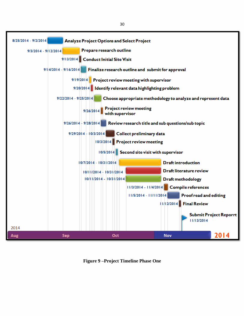
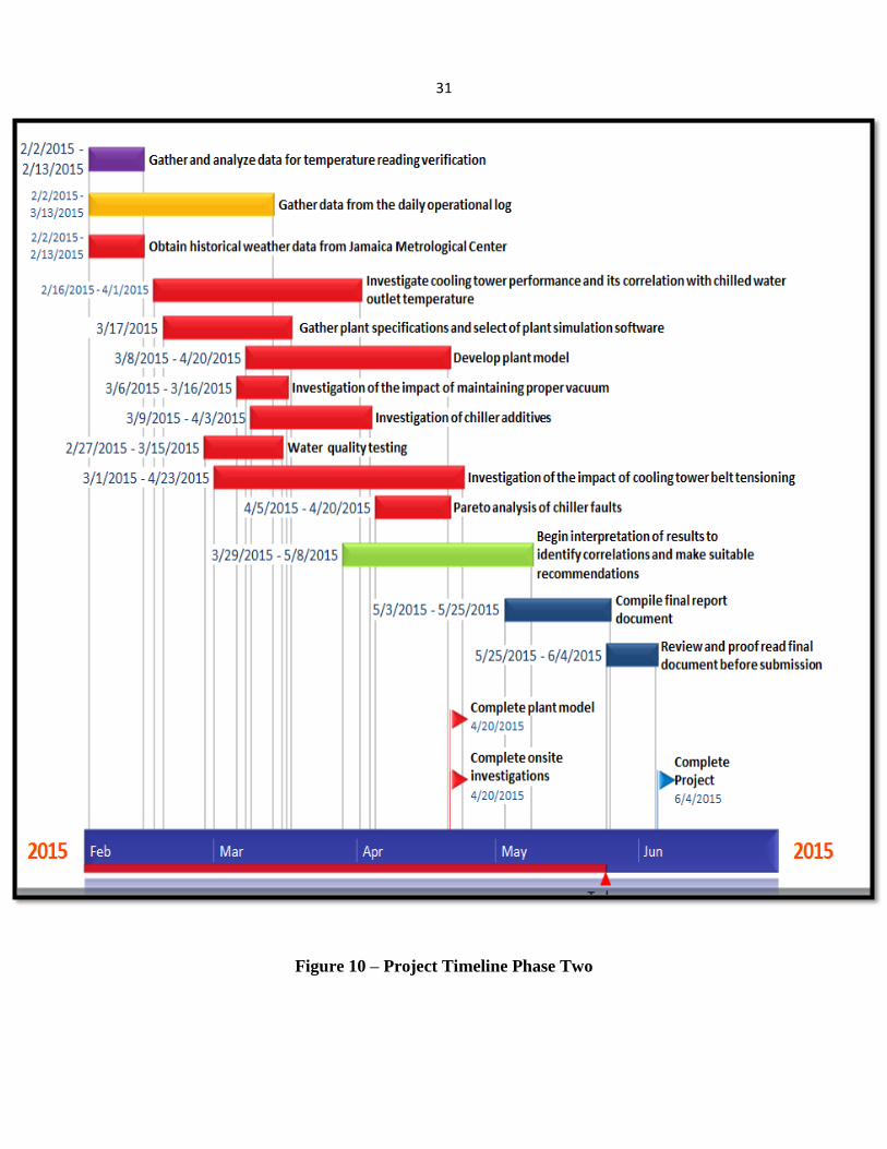
statistically stable, predictable and meets contractual requirement. The project was broken into
two phases, Phase One (research proposal phase) and Phase Two (research investigation phase).
These phases are shown in the following Gant charts.
30
Figure 9 –Project Timeline Phase One
31
Figure 10 – Project Timeline Phase Two
32
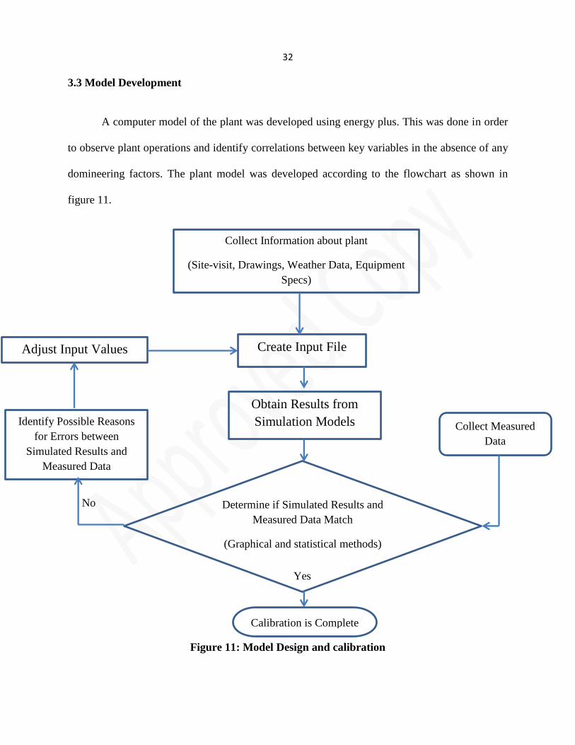
3.3 Model Development
A computer model of the plant was developed using energy plus. This was done in order
to observe plant operations and identify correlations between key variables in the absence of any
domineering factors. The plant model was developed according to the flowchart as shown in
figure 11.
No
Yes
Figure 11: Model Design and calibration
Collect Information about plant
(Site-visit, Drawings, Weather Data, Equipment
Specs)
Calibration is Complete
Adjust Input Values Create Input File
Obtain Results from
Simulation Models
Determine if Simulated Results and
Measured Data Match
(Graphical and statistical methods)
Identify Possible Reasons
for Errors between
Simulated Results and
Measured Data
Collect Measured
Data
33
As illustrated, in developing the system model data was collected about the plant in the
form of technical drawings outlining the equipment onsite and how they are interconnected,
equipment specifications and also weather data. This information was entered into the system to
create the input file. Other information regarding the systems performance was collected from
the daily operational log. Simulations were run, and the model recalibrated until the model was
within an acceptable range with that of the measured data.
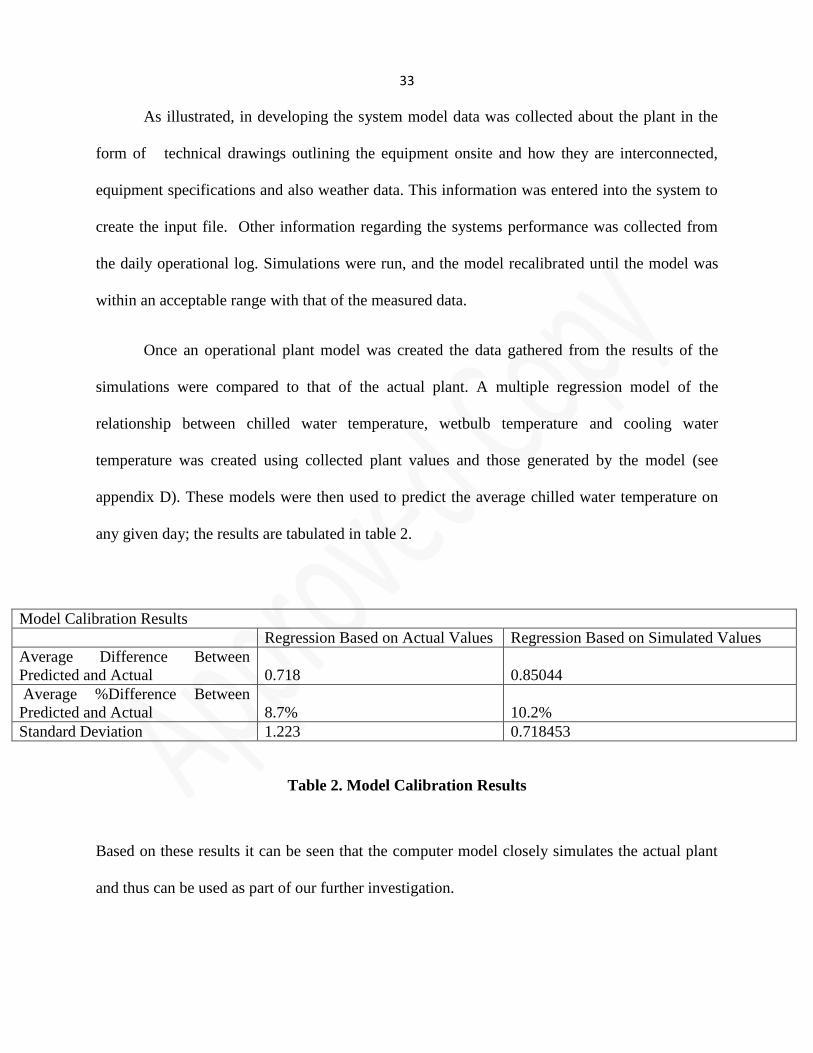
Once an operational plant model was created the data gathered from the results of the
simulations were compared to that of the actual plant. A multiple regression model of the
relationship between chilled water temperature, wetbulb temperature and cooling water
temperature was created using collected plant values and those generated by the model (see
appendix D). These models were then used to predict the average chilled water temperature on
any given day; the results are tabulated in table 2.
Model Calibration Results
Regression Based on Actual Values Regression Based on Simulated Values
Average Difference Between
Predicted and Actual
0.718
0.85044
Average %Difference Between
Predicted and Actual
8.7%
10.2%
Standard Deviation 1.223 0.718453
Table 2. Model Calibration Results
Based on these results it can be seen that the computer model closely simulates the actual plant
and thus can be used as part of our further investigation.
34
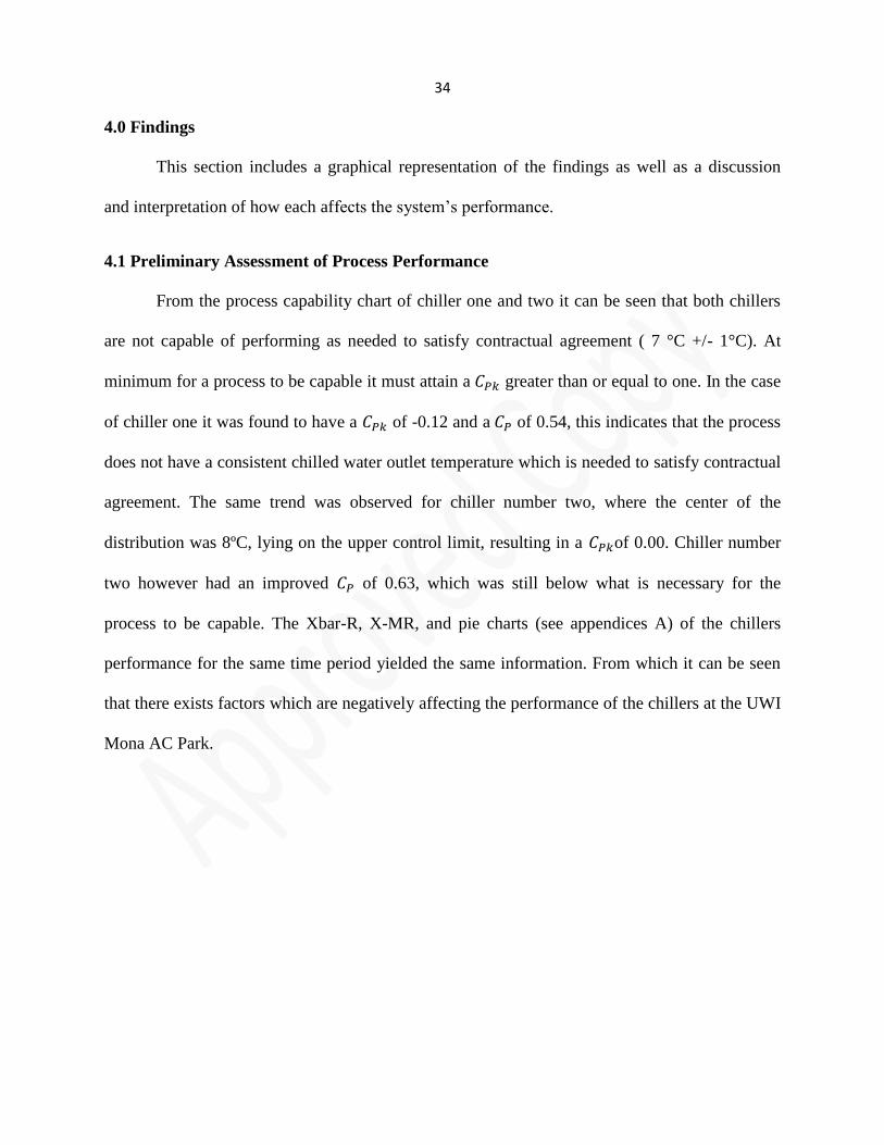
4.0 Findings
This section includes a graphical representation of the findings as well as a discussion
and interpretation of how each aff ’ f
4.1 Preliminary Assessment of Process Performance
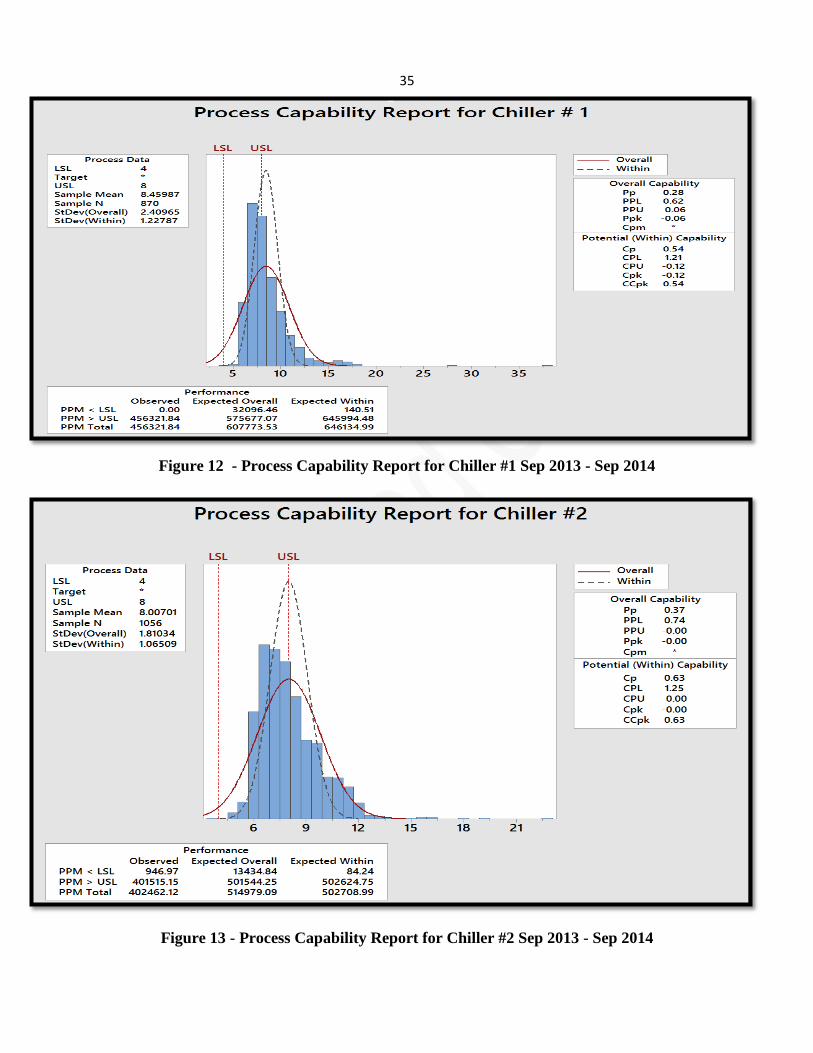
From the process capability chart of chiller one and two it can be seen that both chillers
are not capable of performing as needed to satisfy contractual agreement ( 7 °C +/- 1°C). At
minimum for a process to be capable it must attain a greater than or equal to one. In the case
of chiller one it was found to have a of -0.12 and a of 0.54, this indicates that the process
does not have a consistent chilled water outlet temperature which is needed to satisfy contractual
agreement. The same trend was observed for chiller number two, where the center of the
distribution was 8ºC, lying on the upper control limit, resulting in a of 0.00. Chiller number
two however had an improved of 0.63, which was still below what is necessary for the
process to be capable. The Xbar-R, X-MR, and pie charts (see appendices A) of the chillers
performance for the same time period yielded the same information. From which it can be seen
that there exists factors which are negatively affecting the performance of the chillers at the UWI
Mona AC Park.
35
Figure 12 - Process Capability Report for Chiller #1 Sep 2013 - Sep 2014
Figure 13 - Process Capability Report for Chiller #2 Sep 2013 - Sep 2014
36
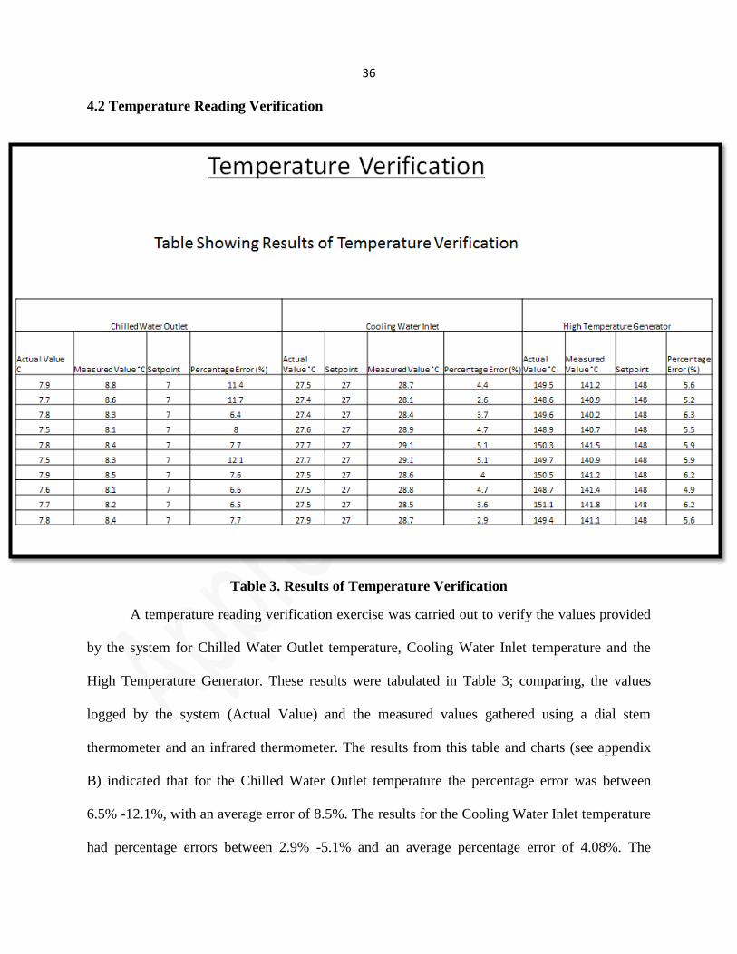
4.2 Temperature Reading Verification
Table 3. Results of Temperature Verification
A temperature reading verification exercise was carried out to verify the values provided
by the system for Chilled Water Outlet temperature, Cooling Water Inlet temperature and the
High Temperature Generator. These results were tabulated in Table 3; comparing, the values
logged by the system (Actual Value) and the measured values gathered using a dial stem
thermometer and an infrared thermometer. The results from this table and charts (see appendix
B) indicated that for the Chilled Water Outlet temperature the percentage error was between
6.5% -12.1%, with an average error of 8.5%. The results for the Cooling Water Inlet temperature
had percentage errors between 2.9% -5.1% and an average percentage error of 4.08%. The
37
results for the High Temperature Generator had percentage errors between 5.2%-6.3% with an
average percentage error of 5.73%. The percentage error between the actual value and the
measured value was due to systematic errors. As described by the Department of Physics and
Astronomy of Appalachian State University (2015), these errors are within an acceptable range
of 10%. Errors were observed in the collection of data. One such error was the inability to insert
the dial stem thermometer at the optimal location. The systems temperature probes were affixed
to these positions in the chilled water loop. The infrared thermometer produced errors due to
thermal radiation being reflected from objects other than the one being measured and also due to
the emissivity wave length setting. From the results ob ’
temperature readings were within an acceptable range of accuracy, Appalachian State University
(2015).
The errors in the measurements taken by the dial stem thermometer are attributed to not
being able to insert the measuring instrument at the optimal locations to take the readings whilst
’ I
the infrared thermometer errors were due to thermal radiation reflected from objects other than
the one being measured and also due to the emissivity wave length setting on thermometer. Thus
from our results it can be seen that the plants temperature parameter readings are within an
acceptable range of accuracy.
38
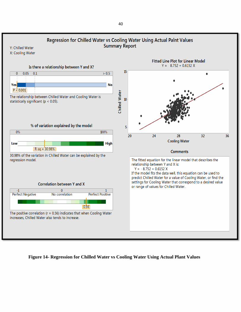
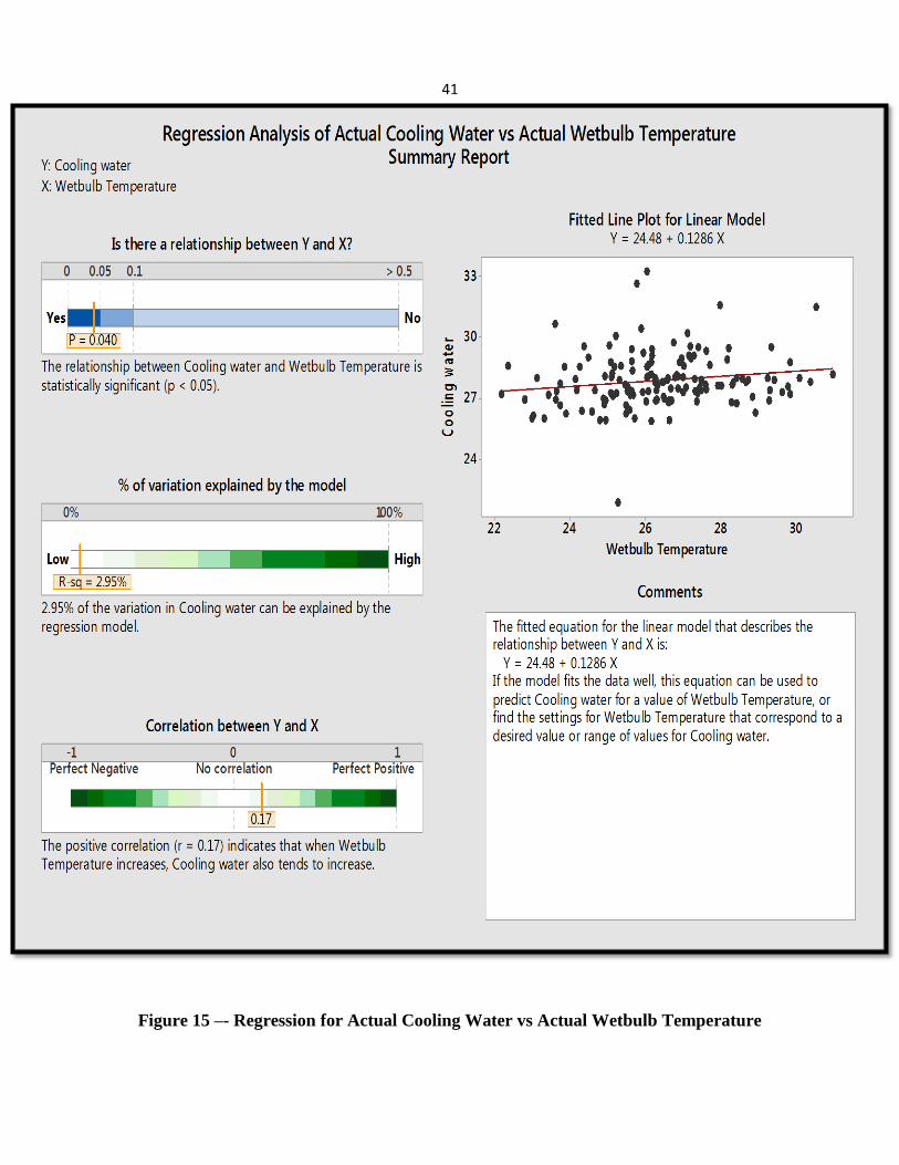
4.3 Regression Analysis of Cooling Water Outlet Temperature, Chilled Water Outlet
Temperature and Wetbulb Temperature
As part of the investigations of cooling tower maintenance and operations, the
performance of the cooling tower and impact of the cooling water inlet temperature on the
chilled water outlet temperature were investigated. A regression model of cooling water inlet
temperature vs. chilled water outlet temperature was made and the results can be seen in Figure
14. From this model it can be seen that there was a moderate correlation between cooling water
inlet temperature and chilled water outlet temperature of 0.56. The test of the null hypothesis of
this model however yielded a value of 0.001, demonstrating a statistically significant
relationship. This correlation was lower than what was expected when compared to evidence
from literature. A regression model of this relationship was also developed using the results from
the energy plus model (see appendix D3) which illustrated a value of 99.73% correlation
’
The test of the null hypothesis of this model yielded a value of 0.001, demonstrating the same
level of a statistically significant relationship. This reveals that there are other unidentified
factors affecting the plant.
Y.A. Li, M.Z. Yu and G.L. Xu, (2001) cited wet bulb temperature as the primary
ff f f I z ’
performance a regression model of cooling water inlet temperature vs. wet bulb temperature was
developed. This model (Figure 15) showed a low positive correlation between cooling water inlet
temperature and wet bulb temperature with a value 3.38% and a statistically significant null
hypothesis value of 0.027. This relationship was also investigated in our model (see appendix
D2). This simulated values showed a moderate positive correlation between cooling water inlet

39
temperature and wet bulb temperature with a value 27.13% and a statistically significant null
hypothesis value of 0.001. Thus, further disparity confirmed that there existed factors on the
plant negatively affecting the performance of the cooling tower and by extension the
achievement of chilled water set point (7 °C` +/- 1°C).
40
Figure 14- Regression for Chilled Water vs Cooling Water Using Actual Plant Values
41
Figure 15 –- Regression for Actual Cooling Water vs Actual Wetbulb Temperature
42
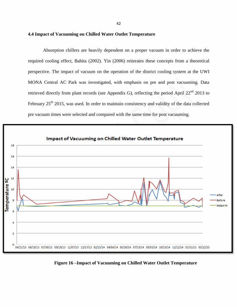
4.4 Impact of Vacuuming on Chilled Water Outlet Temperature
Absorption chillers are heavily dependent on a proper vacuum in order to achieve the
required cooling effect, Bahita (2002). Yin (2006) reiterates these concepts from a theoretical
perspective. The impact of vacuum on the operation of the district cooling system at the UWI
MONA Central AC Park was investigated, with emphasis on pre and post vacuuming. Data
retrieved directly from plant records (see Appendix G), reflecting the period April 22nd
2013 to
February 25th
2015, was used. In order to maintain consistency and validity of the data collected
pre vacuum times were selected and compared with the same time for post vacuuming.
Figure 16 –Impact of Vacuuming on Chilled Water Outlet Temperature
43
Figure 16 illustrates the improvement in chilled water outlet temperature post vacuuming
exercises. An average improvement 1.242ºC in chilled water outlet temperature was noted.
Figure 16 three distinct plots are derived; chilled water outlet before vacuuming, chilled water
outlet temperature after vacuuming and the set point value. The relationship between pre and
post vacuuming is quite notable from the plots, where majority of post vacuum points fell below
the pre vacuum points indicating the improved effect of vacuuming on the chilled water outlet
temperature.
4.5 Chiller Additives
Our investigations revealed that there exists an adequate programme in place to address
the management of chiller additives. Quarterly samples of the LiBr solution are taken and sent to
the OEM and a report (see appendix O1) is sent back. This report indicates what type and how of
each additive should be added to the LiBr solution.
4.6 Cooling Tower Maintenance and Operations
4.6.1 Cooling Tower Effectiveness
Figure 17 illustrates the fluctuations in cooling tower effectiveness over 127 days. The
average cooling tower effectiveness was found to be 70.85%, which is within industry standards
as identified by engineering consultant firm Martech Systems Inc.(2009). However, the graph
’ ff f
between 21.33% and 99.96%, with a standard deviation of 17.49. These large fluctuations in
cooling tower effectiveness indicate that there are factors negatively affecting the cooling tower
performance.
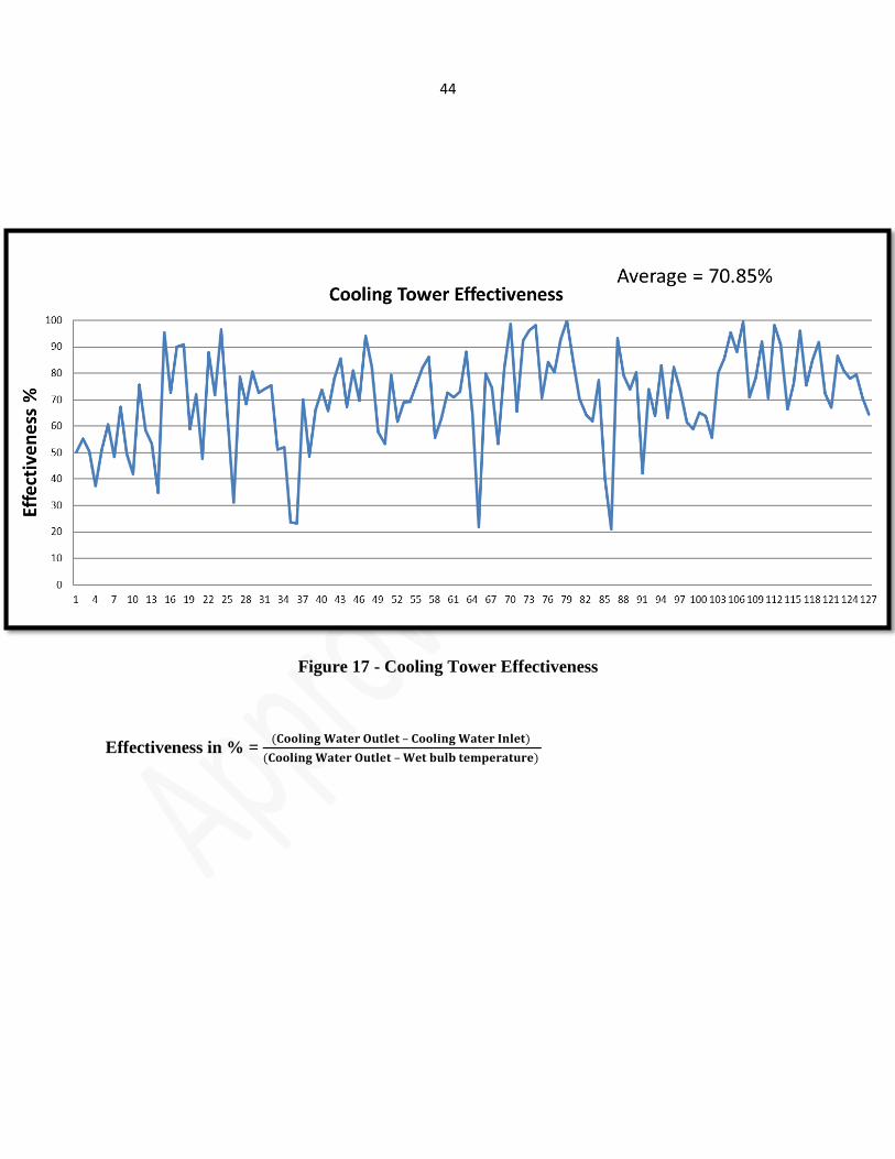
44
Figure 17 - Cooling Tower Effectiveness
Effectiveness in % = –
–
45
4.6.2 Cooling Tower Water Quality
*Best Management Practice and Guidance Manual for Cooling Towers (2005)
Table 4- Results of Water Tests
Four cooling water quality parameters were tested; pH, Conductivity, Hardness and Total
Dissolved Solids (TDS). The TDS values, as outlined by table 4 were within range of best
practices. The pH values for Make-up Water and Cooling Tower one were within range of best
practices and OEM standards however, the pH values for the remaining cooling towers were
46
above OEM standards. Conductivity and hardness, for all four cooling towers and Make-up
Water were above best practice and OEM recommendations.
A contributing factor to the high conductivity values in the cooling tower water was the
high conductivity of the Make- up Water entering the system. A second contributing factor was
the absence of an automatic blow down system, hence, manual blow down being employed. As a
result of this, the system is unable blow down as needed to keep the conductivity within
specified range. According to JEA (2005), these high values of conductivity also negatively
impact the other water parameters measured. Increase in conductivity adversely affects the heat
transfer capabilities of the system by increasing scale build up in the system (see appendix E).
4.6.3 Number of Cooling Water Cycles
The number of cycles can be determined by the ratio of cooling tower conductivity and the
makeup water conductivity.
From our calculations it was found that the system was running at 6 cycles. This is the upper
limit as outlined by JEA (2005).At this level there exists the possibility of increased scale build-
up in the condenser copper tubes, the presence of which, adversely impacts the heat transfer
47
0
2
4
6
8
10
12
14
Tem
pe
ratu
re º
C
Impovement in Chilled Water Outlet Post Belt Tesioning
CHW After
CHW Before
CHWSetpoint
capabilities of the system. According to JEA (2005), operating at a high number of cycles results
in high conductivity and increased water hardness, as seen in table 4.Cooling water best practices
at various cycles can be seen in appendices P1 and P2.
4.6.4 Improvement in Chilled Water Outlet Temperature Post belt Tensioning
It was observed that chilled water outlet temperature approached chilled water set point
(7 °C +/- 1°C) after belt tensioning as outlined by the graph. From figure 18 it can be seen that
there is an improvement in the chilled water outlet temperature post belt tensioning. An average
improvement of 2.56 0C was noted for the 2 year span. A standard deviation of 1.33 was
calculated on the post belt tensioning temperature readings
Figure 18 –Improvement in Chilled Water Outlet Post belt Tensioning
Over a 2 year span it can be interpreted from the Figure F1 (see appendix F) that belt
tensioning also had a direct impact on Cooling Water inlet temperature. Belt tensioning reduced
48
the temperature of the cooling water inlet temperature and as such increased the ability of this
water to absorb more heat from the chiller; hence reducing the chilled water outlet temperature.
The overall average improvement was 1.85 0C before and after tensioning. Belt tension resulted
’ f 0C. A standard deviation of
1.06 was calculated as the difference before and after temperature readings.
4.6.4 Number of Cooling Tower Fan Belts Verification
An investigation was conducted on the number of belts designed to work on the cooling
tower as compared to the number of belts presently used in the operation of the system. The
motor used on the system has a power rating of 18.5 Kw (25hp), and the belt (5vx1400) has a
service factor of 1.2. This information was used to calculate the design power. This was done by
calculating the product of the motor power and the service factor of the belt, which was found to
be 30hp. The design power was then used to calculate the number of belts required to operate the
cooling tower fan effective and efficiently. Based on the calculation it was shown that the tower
system was designed to use 7 belts for proper cooling tower operation according to manufacture
specifications.
It was discovered that presently the tower system operates with 4 or 5 belts. A calculation
was done to find the effects this would have on the operation of the system. The results showed
that using 4 or 5 belts caused each belt to transmit power and stresses above its design
specification. This results in belt failure within about half or less its required life cycle as shown
’ f d a decrease in the effectiveness
of the tower fan operation and an increase in the cooling water inlet temperature. This results in
an increase in the chill water outlet temperature.
49
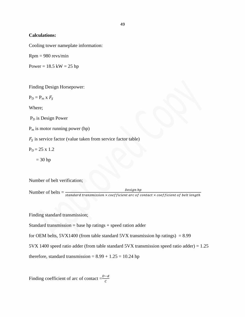
Calculations:
Cooling tower nameplate information:
Rpm = 980 revs/min
Power = 18.5 kW = 25 hp
Finding Design Horsepower:
PD = Pm x
Where;
PD is Design Power
Pm is motor running power (hp)
is service factor (value taken from service factor table)
PD = 25 x 1.2
= 30 hp
Number of belt verification;
Number of belts =
Finding standard transmission;
Standard transmission = base hp ratings + speed ration adder
for OEM belts, 5VX1400 (from table standard 5VX transmission hp ratings) = 8.99
5VX 1400 speed ratio adder (from table standard 5VX transmission speed ratio adder) = 1.25
therefore, standard transmission = 8.99 + 1.25 = 10.24 hp
Finding coefficient of arc of contact =

50
Coefficient of arc of contact =
Coefficient of arc of contact = 0.468
Finding coefficient of belt length found from table to be 0.93
Therefore;
Number of belts =
Number of belts = 6.73
This confirms the 7 belts required for proper tower operation according t f ’
specification.
4.6.5 Failure Mode Effect Analysis (FMEA)
The plant records showed that belt maintenance over the period of 2013 to 2015.
Therefore, an investigation was done on the belts using a failure mode effect analysis (see
appendix H). The analysis focused on the belt failure, severity, occurrence, detection, criticality
and risk priority. The detection, severity and occurrence were given a ranking from 1 to 5. The
modes of failure (see Appendix I) that were analyzed were plastic deformation, tensile breaks,
rapid side wall wear, and belt crimp failure. The analysis showed fatigue failure with the highest
risk priority and criticality. The fatigue failure of the belts will result in an increased cooling
water inlet temperature and hence, an increase in chilled water outlet temperature. Fatigue failure
can be detected through frequent visual inspection of the belts and monitoring of parameters. The
second highest cause of failure was inadequate belt installation. The failure effect is that the belt
teeth will ride on the sprocket. This is detected through inspection of the belt. Shock loading was
another cause of failure with effects similar to fatigue failure. This can be detected by inspection
51
of the cooling tower belts. The fourth cause of failure was the excessive tensioning of the belts.
The effects were worn belt and plastic deformation, and as a result less heat was dissipated
through the tower. The fifth cause of failure was belt mishandling. The effect of this was large
compressive force being exerted on the belts. This was detected by belt inspections. These were
the five highest causes of failure that needed special attention in order to improve the life of the
belts and get the best out of the tower operation.
An interview was conducted with plant personnel on how they installed and maintained
tower belts. It was discovered that the tower belts were just placed on the pulley and tension
based on human judgment. There is no tension meter available to check the actual tension of the
belts; nor was there the ability to inspect the alignment of the pulleys. Both are necessary for
proper belt operation.
Best practices and standards recommend that operators should never replace one belt in a
set, but instead replace all belts. All belts are required to transmit a design torque. When
replacing belts, it may be necessary to loosen the belt tension ram since new belts are not
stretched out. Tension of the belts is critical and the best tension for a V-belt is the lowest at
which the belts will not slip under the higher load condition. Therefore, the tension of the belts
must be checked frequently during the first day of operation. This is important because too much
tension shortens belt life. Keeping belts and sheaves free from foreign material can help prevent
belt slippage. If a belt slips, ’
Based on the comparison between best practices and how plant technicians performed belt
maintenance; it was discovered that the present operation on the tower belts lacked proper
equipment and technique. Proper equipment and technique will help improve belt life-span,
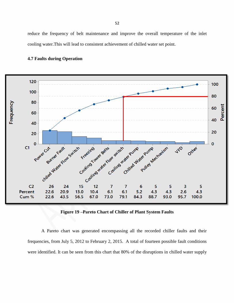
52
reduce the frequency of belt maintenance and improve the overall temperature of the inlet
cooling water.This will lead to consistent achievement of chilled water set point.
4.7 Faults during Operation
Figure 19 –Pareto Chart of Chiller of Plant System Faults
A Pareto chart was generated encompassing all the recorded chiller faults and their
frequencies, from July 5, 2012 to February 2, 2015. A total of fourteen possible fault conditions
were identified. It can be seen from this chart that 80% of the disruptions in chilled water supply

53
was cause by Power cuts, Burner Faults, Freezing, Cooling Tower Belt Failure and Cooling
Water Flow Switch failure.
54
5.0 Conclusions
f j f
J 0 M 0 , f :
1. k f f -0 0
f f k <
2. x- x- f f
3. S 66% 0 3 0 f # f #
6 %, ’ f
4. The three major temperature parameters most likely to indicate inconsistencies with the
system were investigated and verified. These parameters were chilled water outlet
temperature, cooling water inlet, and high temperature generator.
5. The average percentage error for each parameter investigated was 8.5%, 4.08% and
5.73% for chilled water outlet, cooling water inlet and high temperature generator
respectively. Systematic Errors were deemed root cause for percentage errors, and were
within acceptable threshold.
6. Regression Analysis, based on computer model yielded greater correlations coefficients
and smaller test of the null hypothesis (p-value) when compared to Regression based on
actual plant values.
7. I f
, f
55
8. Water Quality Parameters; conductivity, hardness andpH fell outside of the minimum
threshold standard for both the OEM and industry standards. TDS were within acceptable
range.
9. Water softener in chiller #1 was found to be defective.
10. Frequent belt failure negatively impacts both chilled water and cooling water
temperature. There wasa 1.848 °C improvement in cooling water inlet temperatures and
2.559 C improvement in chilled water outlet temperature post belt maintenance.
11. From FMEA fatigue failure, inadequate belt installation, shock loading, belt mishandling
and foreign objects between sheaves and belt accounted for the highest RPN.
12. The average cooling tower effectiveness was calculated to be 70.85%.Industry standards
stipulate between 70 and 75 %, however large fluctuations were noted.
13. An adequate programme is in place to address the management of chiller additives, which
is in collaboration with OEM.
14. The Six faults; power cut, burner fault, chilled water flow switch , freezing, cooling
tower belt failure, and cooling water flow switch account for 80% of disruptions in
cooling.
15. f
16. Scale build-up noted on scale indicator confirming poor water quality.
17. Adequate program in place to address the management of chiller additives, in
collaboration with original equipment manufacturer (OEM).
I k j f j ,
A , f

56
, f
f k f q
f H z ff f
f f ,
- f
57
6 Recommendations
The recommendations are as follows:
1. Conduct quarterly statistical analysis of plant performance, by conducting regression
analysis, process capability analysis and pie chart showing the achievement of days set
point met over the period.
2. Include wet bulb temperature on the daily operation log to aid statistical analysis.
3. I
f
4. De-scale condenser tubes annually to improve heat rejection and heat transfer capabilities
of the cooling system.
5. Use the correct number of belts (7 belts) and type 5VX1400 as specified by OEM and as
confirmed through calculations from investigations conducted.
6. Put measures in place to minimize or eliminate the recurrence of identified six critical
faults during operation.
7. Implement robust and routine water treatment regime, which includes:
Scheduled automated injection of chemical treatment as per OEM specifications
Routine monthly cleaning of cooling tower and auxiliary components
Repair defective water softener in an effort to improve water quality
Automate blow down process according to system design
Include specific guidelines addressing chemical substitution optimize chemical
treatment dosage.
Test cooling tower water daily to control number of cycles.
58
Effluent and influent flow meters to monitor cooling performance.
8. Utilize CMMS as an intelligent agent as part of the RCM program to aid in the
preventative, predictive and conditioned based maintenance activities to reduce MTTF of
the system.
9. Create a data warehouse to collect large amounts of data that will support decision
making.
10. Acquire and utilize precision instruments such as tension meter and laser alignment tool
as part of cooling tower belt maintenance and operation.
The recommendations outlined present an opportunity for the technical operators at the UWI
Mona AC Park to implement a standardized program to keep the plant under statistical process
control. It outlines metrics by which key parameters can be monitored and highlights
programsthat can be put in place to manage the identified factors which negatively affect the
achievement of chilled water set point(7ºC +/- 1°C). Further studies in this area may
investigatethe factors inherit to the distribution system and energy transfer station (ETS), the
subsequent impact each has on the achievement of chilled water set point.
59
References
Allen, M. P. (2007). Understanding Regression Analysis. Springer Science & Business Media.
American Society of Heating, Refrigerating and Air-Conditioning Engineers. (2008). Ashrae
Handbook: HVAC Systems and Equipment, I-P Edition. American Society of Heating,
Refrigerating and Air-Conditioning Engineers.
Appalachian State University. (2015). Error Analysis. Retrieved from appstate.edu:
http://physics.appstate.edu/undergraduate-programs/laboratory/resources/error-analysis
ASHRAE. (2004). ASHRAE:Standard 90.1 . Retrieved from ASHRAE:
https://www.ashrae.org/resources--publications/bookstore/standard-90-1
Balbach, E. D. (1999). Using Case Studies to do Program Evaluation. Retrieved from
http://www.case.edu/affil/healthpromotion/ProgramEvaluation.pdf
Bhaita, A. (2012). Retrieved from Overview of Vapor Absorption Chilling Systems:
http://www.pdhonline.org/courses/m130/m130content.pdf
Black, K. (2011). Business Statistics: For Contemporary Decision Making. John Wiley & Sons.
Cengel, Y., & Boles, M. (2011). Thermodynamics: An Engineering Approach. McGraw-Hill
Professional Publishing.
Clugston, M., & Flemming , R. (2000). Advanced Chemistry. OUP Oxford.
Conservation Project office ,UWI Mona, Jamaica. (n.d.). Energy Conservation Project.
Retrieved from University of the West Indies, Mona, Jamaica:
http://www.mona.uwi.edu/emd/sites/default/files/emd/uploads/Energy%20managment%2
0at%20mona%20-an%20Overview.pdf
Conservation Project office, U. M. (2010, March). A.C. Policy. Retrieved from University of the
West Indies, Mona, Jamaica:
http://www.mona.uwi.edu/bursary/sites/default/files/bursary/C_Policy_Document_-
_First_Edition_March_2010.pdf
Energy Design Resources. (2009, December). Design Guidelines: CoolTools Chilled Water
Plant. Retrieved from Energy Design Resources:
http://energydesignresources.com/resources/publications/design-guidelines/design-
guidelines-cooltools-chilled-water-plant.aspx
Euroheat and Power. (2006, May). District Cooling : Cooling More With Less. Retrieved from
Euroheat and Power:
60
http://www.google.com.jm/url?sa=t&rct=j&q=&esrc=s&source=web&cd=1&cad=rja&u
act=8&ved=0CB4QFjAA&url=http%3A%2F%2Fwww.euroheat.org%2FAdmin%2FPub
lic%2FDWSDownload.aspx%3FFile%3D%2FFiles%2FFiler%2Fdocuments%2Fposition
papers%2FDistrict_Cooling%2FEHPCoolingMore
Euroheat and Power. (2012, September 8). District Heating and Cooling: strategic Research
Agenda. Retrieved from Euroheat and Power: http://www.dhcplus.eu/wp-
content/uploads/2012/05/120529_DHC+SRA_final.pdf
Evans, J. R., & Lindsay, W. (2012). Managing for Quality and Performance Excellence (Vol.
VIII). Cenage Learning.
Fischler, A. S. (2014). Mixed Methods. Retrieved from
http://www.fischlerschool.nova.edu/Resources/uploads/app/35/files/ARC_Doc/mixed_m
ethods.pdf
George, M. L., Rowlands, D., & Price, M. (2005). The Lean Six Sigma Pocket Tool Book.
McGraw-Hill.
Herold, E. K., Radermacher, R., & Sanford, A. (1996). Absorption Chillers and Heat Pumps.
CRC Press.
Hiregoudar, C. (2007). Facility Planning And Layout Design. Technical Publications.
kaushik, S., & Singh, D. S. (2014). Thermodynamic Analysis of Vapor Absorption Refrigeration
System and Calculation of COP. International journal for Research In applied Science
and Engineering Technology, II(2), 73-80.
Klenke, K. (2008). Qualitative Research in the Study of Leadership. Emerald Group Publishing.
Liptak, B. G. (2007, Bela G. Liptak). Instrument Engineers' Handbook, Fourth Edition, Volume
One: Process Measurement and Analysis. CRC Press.
Mansour, F. (2014, July). Performance Improvement of a Forced Draft Counter Flow Cooling
Tower. Retrieved from Linkedin:
https://www.linkedin.com/pulse/article/20140701054104-104030228-performance-
improvement-of-a-forced-draft-counter-flow-cooling-tower-coupled-to-an-air-
conditioning-system-in-a-hot-humid-environment
Mather, D. (2002). CMMS: A Timesaving Implementation Process. CRC Press.
Maytal, B.-Z., & Pfotenhauer, J. M. (2012). Miniature Joule-Thomson Cryocooling: Principles
and Practice. Springer Science & Business Media.
61
Melbourne,Australia :Department of Human Services. (January, 2002). Code of Practice for
Water Treatment. Retrieved from Department of Human Services: Australia:
https://www.google.com.jm/url?sa=t&rct=j&q=&esrc=s&source=web&cd=1&cad=rja&
uact=8&ved=0CCEQFjAA&url=https%3A%2F%2Fwww.infomil.nl%2Fpublish%2Fpag
es%2F70361%2Fcoolingtowersystems_codeofpracticeaustralia.pdf&ei=ovtoVICvJMvls
ATazoDABQ&usg=AFQjCNF8Bh86NC2ie4IQ
Miller, M., & Miller, R. (2006). Air Conditioning and Refrigeration, Second Edition. McGraw
Hill Professional.
Moss, A. (2011, September 19). Climatologist: Demand for more cooling will increase energy
use. Retrieved from JamaicaGleaner.com: http://jamaica-
gleaner.com/latest/article.php?id=32026
Myron L Company. (2013). ULTRAMETER II™ 6PFCE and 4P. Retrieved October 2014, from
http://www.myronl.com/products/ultrameter_II.htm
Northwest Energy Efficiency Alliance. (2004). Operation and Maintenance of Chillers .
Retrieved from BetterBricks.com:
http://www.betterbricks.com/graphics/assets/documents/BOpEqSysChillers.pdf
Piper, J. E. (1999). Operations and Maintenance Manual for Energy Management. M.E. Sharpe.
Reshid, M. N., & Abd Ma, M. A. (2011). Availability and reliability modelling for chilled water
generation of a cogenerated power plant using multi-state system theory. Petronas
University of Technology:The 2011 National Postgraduate Conference. Petronas
University of Technology.
Rockwell, K., & Lee, J. (2012). Wet Bulb Temperature and Its Impact on Building Performance.
Retrieved from http://atsiteinc.com/wp-
content/uploads/2012/05/BrainFood_WetBulbTemp.pdf
Severini, S. C. (2004, July). Primary-Secondary Chilled Water Systems. ASHRAE Journal, 27-
31.
Skagstasd, B., & Mildenstein, P. (2002). District Heating and Cooling Connection Handbook.
International Energy Agency (IEA).
Southern California Gas Company,New Buildings Institute. (1998). Absorption Chillers. New
Buildings Institute.
Stanford III, H. W. (2011). HVAC Water Chillers and Cooling Towers: Fundamentals,
Application, and Operation. CRC Press.
Swanborn, P. (2010). Case Study Research: Why, Why and How? SAGE.
62
The United Sates Environment Protection Agency. (2012, March 06). Water: Monitoring &
Assessment . Retrieved November 1, 2014, from The United Sates Environment
Protection Agency: http://water.epa.gov/type/rsl/monitoring/vms59.cfm
The University Of North Carolina at Chapel Hill :Department of Facilities Planning &
Construction. (2010). Chilled Water Design Specifications. Retrieved from The
University Of North Carolina at Chapel Hill:
http://maps.unc.edu/guidelinespdf/Chilled%20Water%20Distibution.pdf
Tomforde, C., & Luke, A. (2012). Experimental Investigations On Falling-Film Absorbers With
Horizontal Tubes – A Review. Retrieved from
http://docs.lib.purdue.edu/cgi/viewcontent.cgi?article=2192&context=iracc
U.S. Department of Energy. (2014). Best Management Practice 10 Cooling Tower Management.
Retrieved from http://energy.gov/eere/femp/best-management-practice-10-cooling-tower-
management.
Vriens, D., & Achterbergh, J. (2010). Organizations: Social Systems Conducting Experiments.
Springer Science & Business Media.
Whitman, W. C. (2002). Dristrict Heating of Vapor Absorption Refrigeration System and
Calculation Of COP, International Journal for Research and Engineering Technology.
Delmar Cengage Learning.
Whitman, W. C., Johnson, W. M., & Tomczuk, J. A. (2009). Refrigeration and Air Conditioning
Technology (Vol. IV). Delmar Cengage Learning.
Wolaver, B. D. (2008). Hydrogeology of the Cuatrocienegas Basin,Coahuila, Mexico: An
Integrative Approach to Arid Karst Aquifier Delineation. ProQuest.
World Watch Institute. (2013). Jamaica Sustainable Energy Roadmap: Pathways to an
Affordable, Reliable, Low-Emission Electricity System. Retrieved from worldwatch.org:
http://www.worldwatch.org/system/files/Jamaica-Sustainable-Energy-Roadmap-
InclAppendices-112013.pdf
Y.A. Li, M. Y. (2001). Analysis of Energy Efficiency of Chiller Operation at Night.
International Journal on Architectural Science, III (1), 18-22.
Yin, H. (2006). An Absorption Chiller in a Micro BCHP Application: Model based Design and
Performance Analysis. Retrieved from
http://www.cmu.edu/iwess/components/steam_absorption_chiller/Thesis_chiller_hongxi_
yin_main_text.pdf
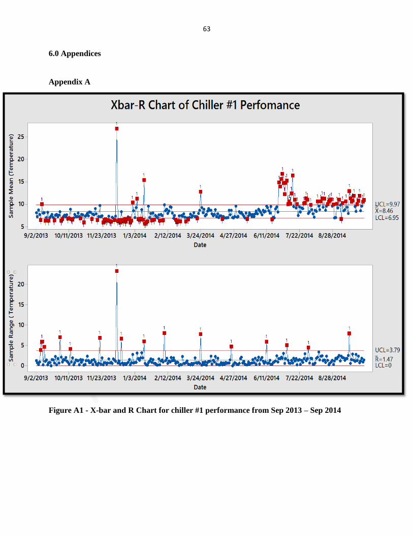
63
6.0 Appendices
Appendix A
Figure A1 - X-bar and R Chart for chiller #1 performance from Sep 2013 – Sep 2014
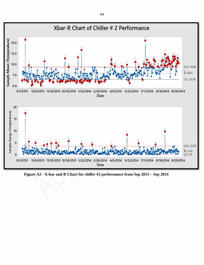
64
Figure A2 - X-bar and R Chart for chiller #2 performance from Sep 2013 – Sep 2014
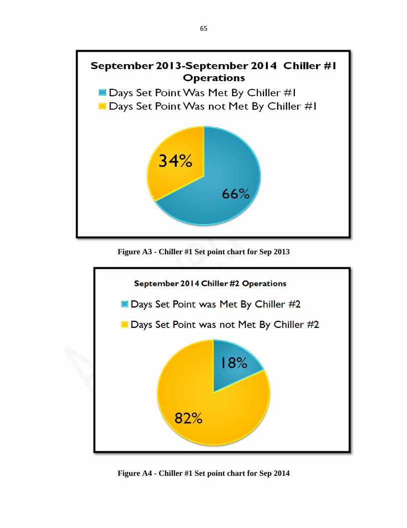
65
Figure A3 - Chiller #1 Set point chart for Sep 2013
Figure A4 - Chiller #1 Set point chart for Sep 2014
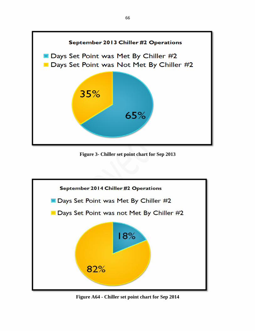
66
Figure 3- Chiller set point chart for Sep 2013
Figure A64 - Chiller set point chart for Sep 2014
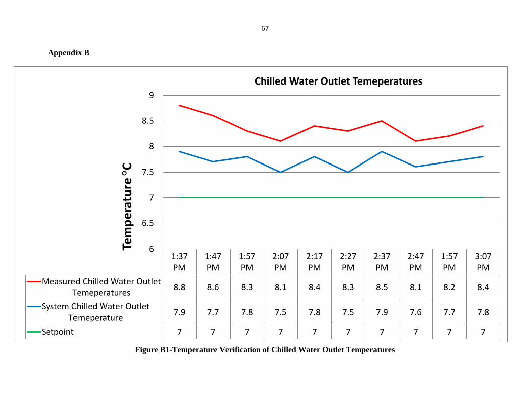
67
1:37PM
1:47PM
1:57PM
2:07PM
2:17PM
2:27PM
2:37PM
2:47PM
1:57PM
3:07PM
Measured Chilled Water OutletTemeperatures
8.8 8.6 8.3 8.1 8.4 8.3 8.5 8.1 8.2 8.4
System Chilled Water OutletTemeperature
7.9 7.7 7.8 7.5 7.8 7.5 7.9 7.6 7.7 7.8
Setpoint 7 7 7 7 7 7 7 7 7 7
6
6.5
7
7.5
8
8.5
9
Chilled Water Outlet Temeperatures
Appendix B
Figure B1-Temperature Verification of Chilled Water Outlet Temperatures
68
1:37 PM 1:47 PM 1:57 PM 2:07 PM 2:17 PM 2:27 PM 2:37 PM 2:47 PM 1:57 PM 3:07 PM
Actual Cooling Water Temeperature 27.5 27.4 27.4 27.6 27.7 27.7 27.5 27.5 27.5 27.9
Cooling Water Inlet Setpoint 27 27 27 27 27 27 27 27 27 27
Measured Cooling Water InletTemeperature
28.7 28.1 28.4 28.9 29.1 29.1 28.6 28.8 28.5 28.7
26.5
27
27.5
28
28.5
29
29.5
Tem
pe
ratu
re °
C
Cooling Water Inlet Temeperatures
Figure B2-Temperature Verification of Cooling Water Outlet Temperatures
69
1:37 PM 1:47 PM 1:57 PM 2:07 PM 2:17 PM 2:27 PM 2:37 PM 2:47 PM 1:57 PM 3:07 PM
Actual HTG Temeperature 149.5 148.6 149.6 148.9 150.3 149.7 150.5 148.7 151.1 149.4
Measured HTG Temperature 141.2 140.9 140.2 140.7 141.5 140.9 141.2 141.4 141.8 141.1
HTG Setpoint 148 148 148 148 148 148 148 148 148 148
138
140
142
144
146
148
150
152
High Temeperature Generator Temperatures
Figure B3-Temperature Verification of High Temperature Generator Temperatures
70
150
620 600
580
620
120 150 150 150 150
50
200 200 200 200
Make-up Water Cooling Tower # 1 Cooling Tower # 2 Cooling Tower # 3 Cooling Tower # 4
Hardness (ppm)
Measured Value Best Practices Manufacturer's Standards
Appendix C
Figure C1-Results of Water Hardness Tests
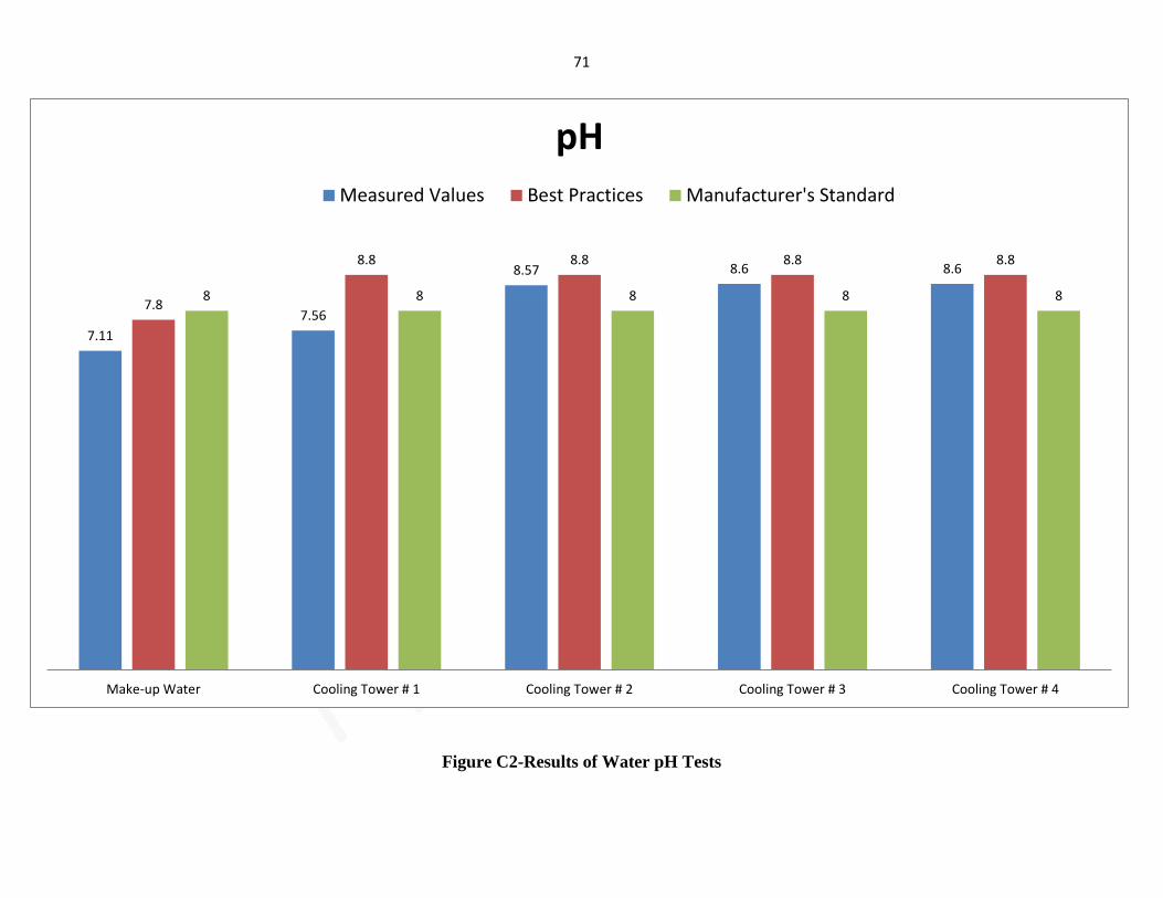
71
7.11
7.56
8.57 8.6 8.6
7.8
8.8 8.8 8.8 8.8
8 8 8 8 8
Make-up Water Cooling Tower # 1 Cooling Tower # 2 Cooling Tower # 3 Cooling Tower # 4
pH
Measured Values Best Practices Manufacturer's Standard
Figure C2-Results of Water pH Tests
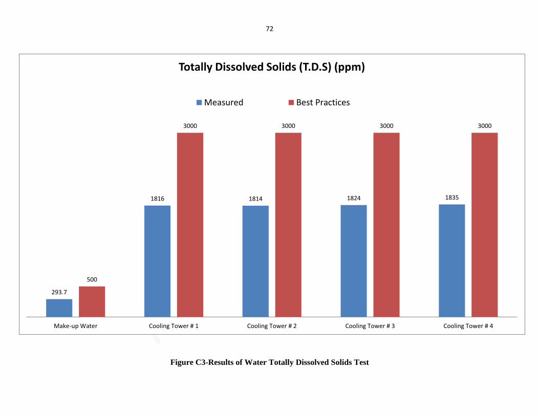
72
293.7
1816 1814 1824 1835
500
3000 3000 3000 3000
Make-up Water Cooling Tower # 1 Cooling Tower # 2 Cooling Tower # 3 Cooling Tower # 4
Totally Dissolved Solids (T.D.S) (ppm)
Measured Best Practices
Figure C3-Results of Water Totally Dissolved Solids Test
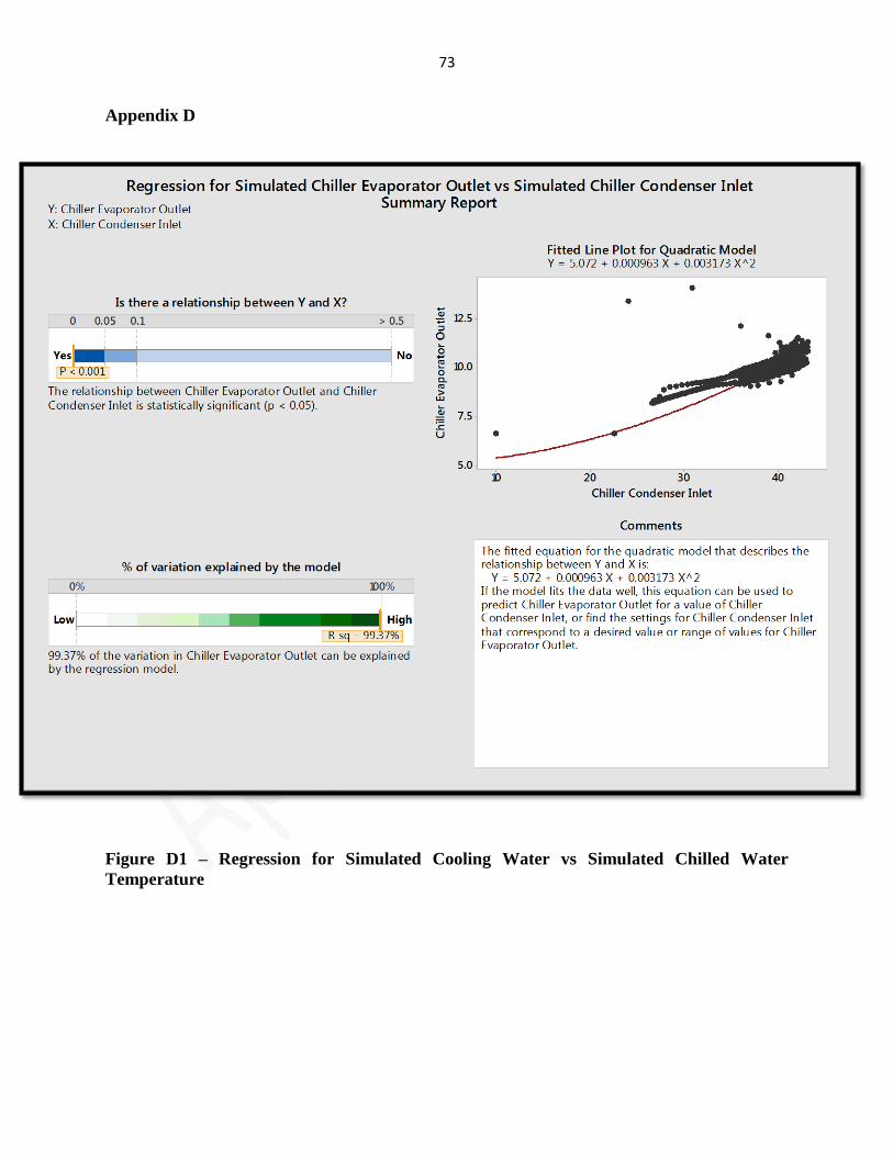
73
Appendix D
Figure D1 – Regression for Simulated Cooling Water vs Simulated Chilled Water
Temperature
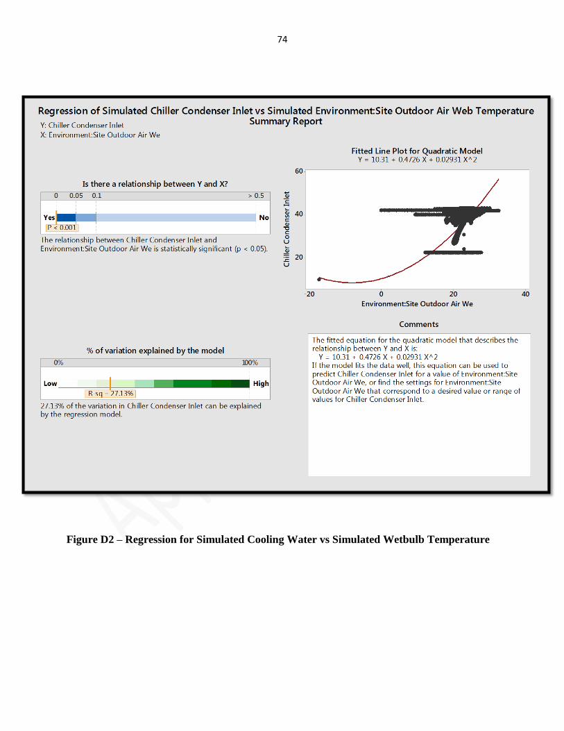
74
Figure D2 – Regression for Simulated Cooling Water vs Simulated Wetbulb Temperature
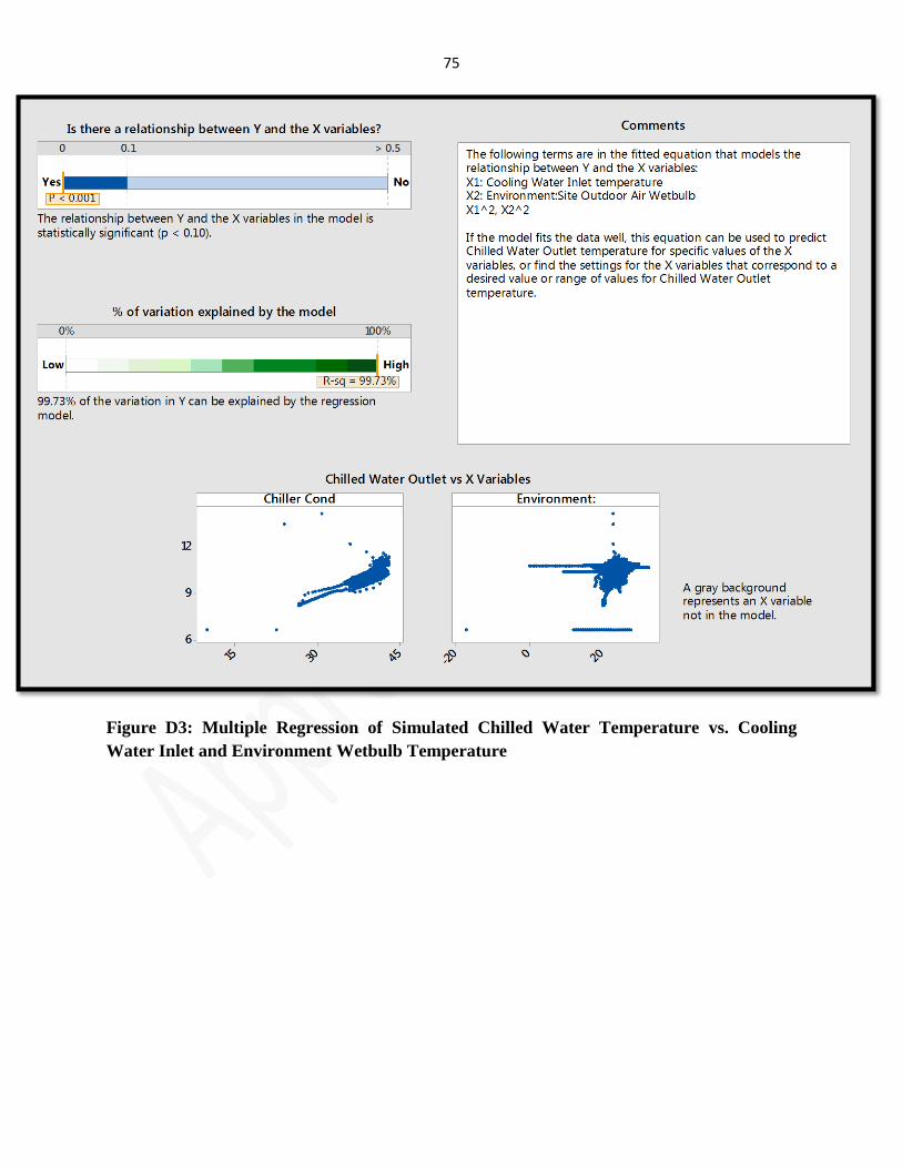
75
Figure D3: Multiple Regression of Simulated Chilled Water Temperature vs. Cooling
Water Inlet and Environment Wetbulb Temperature
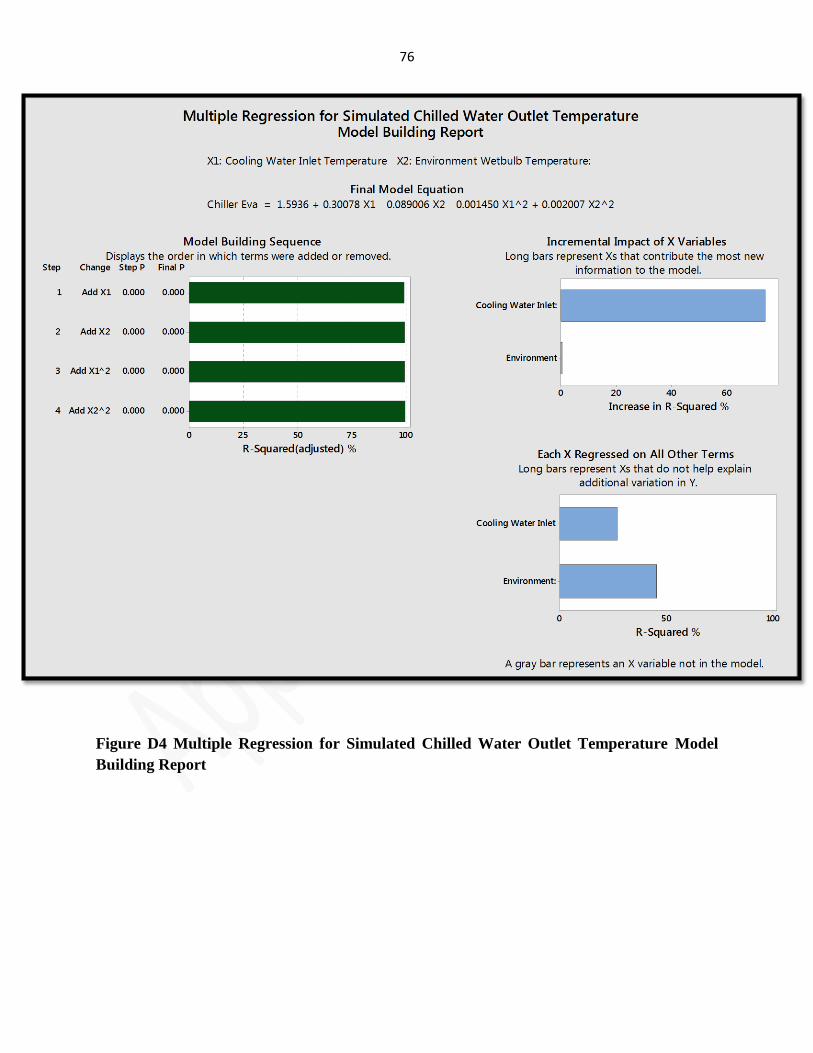
76
Figure D4 Multiple Regression for Simulated Chilled Water Outlet Temperature Model
Building Report
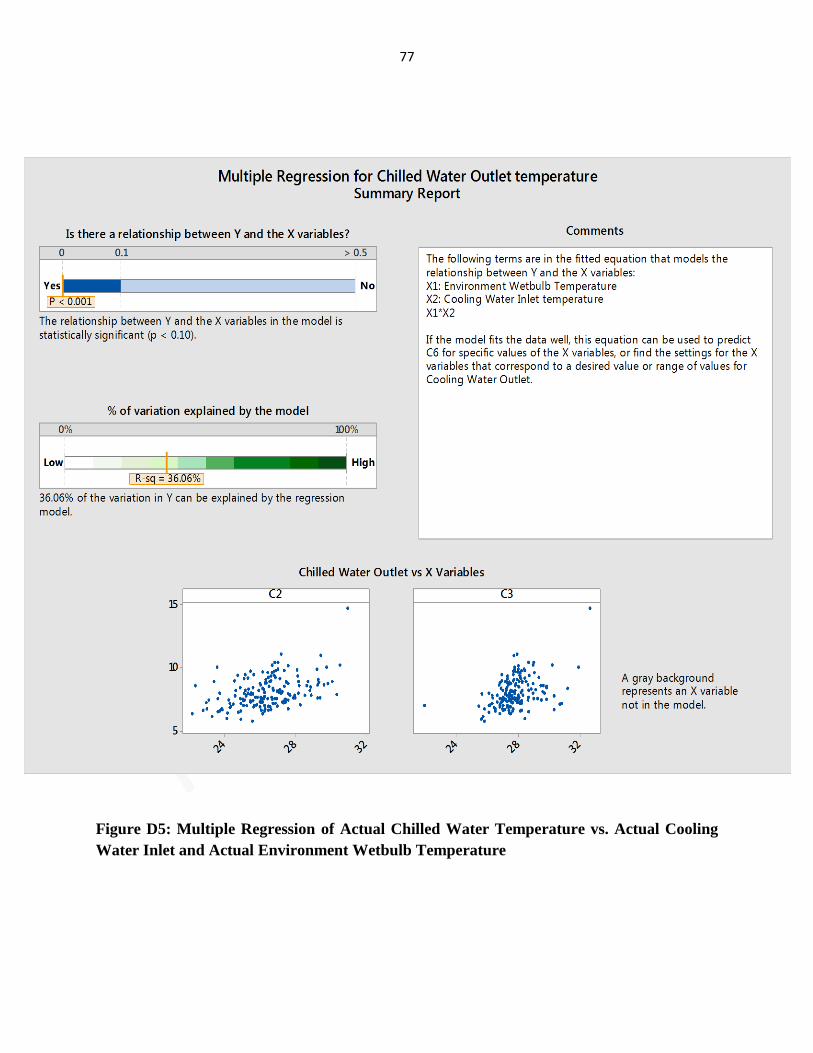
77
Figure D5: Multiple Regression of Actual Chilled Water Temperature vs. Actual Cooling
Water Inlet and Actual Environment Wetbulb Temperature
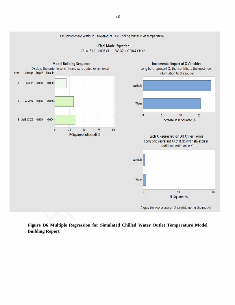
78
Figure D6 Multiple Regression for Simulated Chilled Water Outlet Temperature Model
Building Report
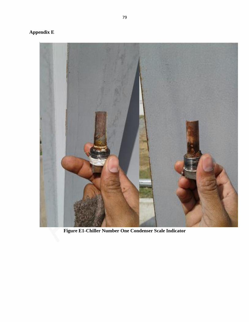
79
Appendix E
Figure E1-Chiller Number One Condenser Scale Indicator

80
Figure E2-Chiller Number One Condenser Scale Indicator
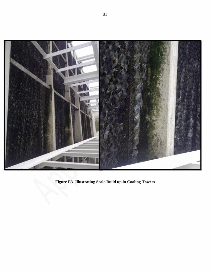
81
Figure E3- Illustrating Scale Build up in Cooling Towers
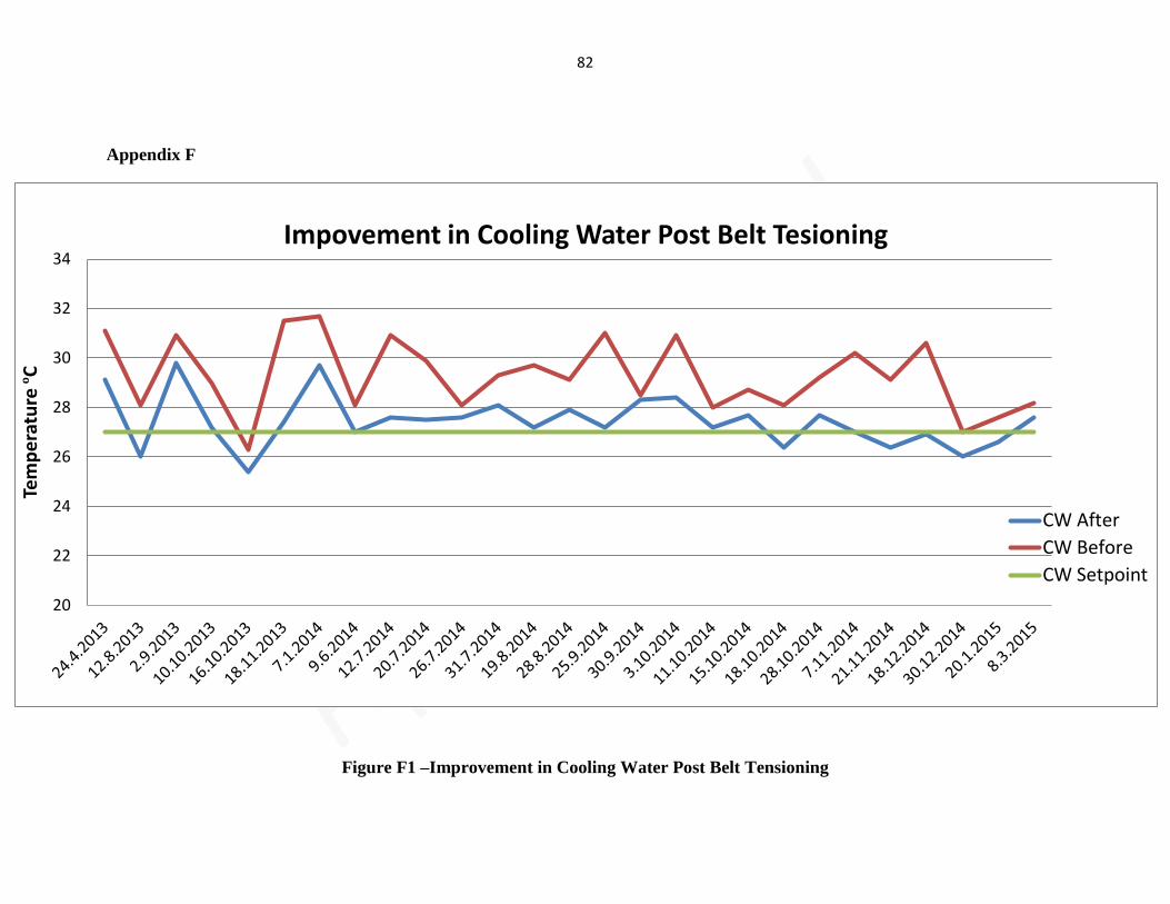
82
20
22
24
26
28
30
32
34
Tem
pe
ratu
re º
C
Impovement in Cooling Water Post Belt Tesioning
CW After
CW Before
CW Setpoint
Appendix F
Figure F1 –Improvement in Cooling Water Post Belt Tensioning
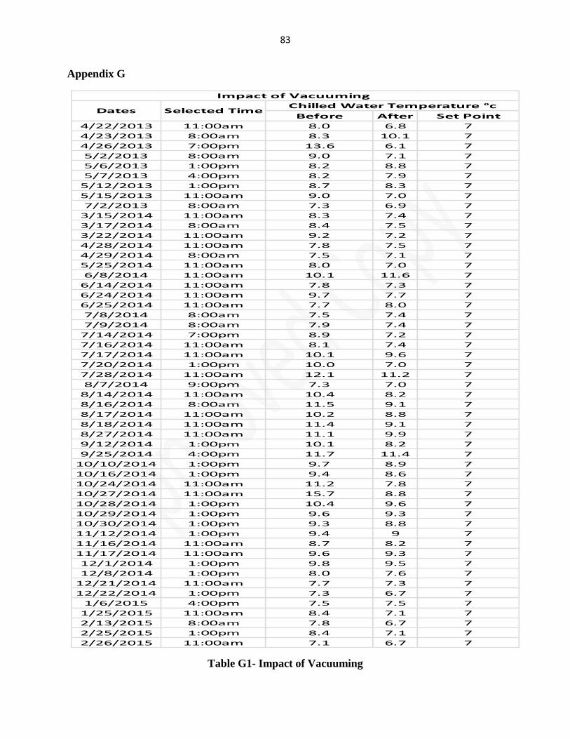
83
Appendix G
Table G1- Impact of Vacuuming
Before After Set Point
4/22/2013 11:00am 8.0 6.8 7
4/23/2013 8:00am 8.3 10.1 7
4/26/2013 7:00pm 13.6 6.1 7
5/2/2013 8:00am 9.0 7.1 7
5/6/2013 1:00pm 8.2 8.8 7
5/7/2013 4:00pm 8.2 7.9 7
5/12/2013 1:00pm 8.7 8.3 7
5/15/2013 11:00am 9.0 7.0 7
7/2/2013 8:00am 7.3 6.9 7
3/15/2014 11:00am 8.3 7.4 7
3/17/2014 8:00am 8.4 7.5 7
3/22/2014 11:00am 9.2 7.2 7
4/28/2014 11:00am 7.8 7.5 7
4/29/2014 8:00am 7.5 7.1 7
5/25/2014 11:00am 8.0 7.0 7
6/8/2014 11:00am 10.1 11.6 7
6/14/2014 11:00am 7.8 7.3 7
6/24/2014 11:00am 9.7 7.7 7
6/25/2014 11:00am 7.7 8.0 7
7/8/2014 8:00am 7.5 7.4 7
7/9/2014 8:00am 7.9 7.4 7
7/14/2014 7:00pm 8.9 7.2 7
7/16/2014 11:00am 8.1 7.4 7
7/17/2014 11:00am 10.1 9.6 7
7/20/2014 1:00pm 10.0 7.0 7
7/28/2014 11:00am 12.1 11.2 7
8/7/2014 9:00pm 7.3 7.0 7
8/14/2014 11:00am 10.4 8.2 7
8/16/2014 8:00am 11.5 9.1 7
8/17/2014 11:00am 10.2 8.8 7
8/18/2014 11:00am 11.4 9.1 7
8/27/2014 11:00am 11.1 9.9 7
9/12/2014 1:00pm 10.1 8.2 7
9/25/2014 4:00pm 11.7 11.4 7
10/10/2014 1:00pm 9.7 8.9 7
10/16/2014 1:00pm 9.4 8.6 7
10/24/2014 11:00am 11.2 7.8 7
10/27/2014 11:00am 15.7 8.8 7
10/28/2014 1:00pm 10.4 9.6 7
10/29/2014 1:00pm 9.6 9.3 7
10/30/2014 1:00pm 9.3 8.8 7
11/12/2014 1:00pm 9.4 9 7
11/16/2014 11:00am 8.7 8.2 7
11/17/2014 11:00am 9.6 9.3 7
12/1/2014 1:00pm 9.8 9.5 7
12/8/2014 1:00pm 8.0 7.6 7
12/21/2014 11:00am 7.7 7.3 7
12/22/2014 1:00pm 7.3 6.7 7
1/6/2015 4:00pm 7.5 7.5 7
1/25/2015 11:00am 8.4 7.1 7
2/13/2015 8:00am 7.8 6.7 7
2/25/2015 1:00pm 8.4 7.1 7
2/26/2015 11:00am 7.1 6.7 7
Selected TimeDatesChilled Water Temperature ºc
Impact of Vacuuming
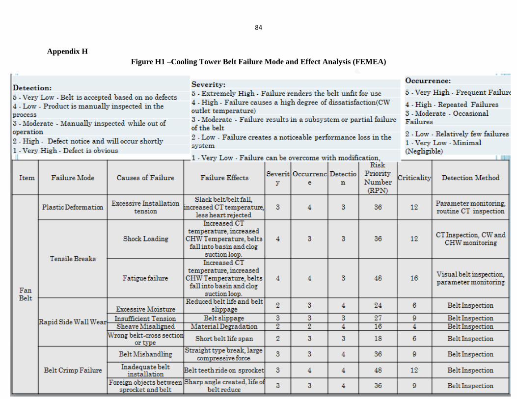
84
Appendix H
Figure H1 –Cooling Tower Belt Failure Mode and Effect Analysis (FEMEA)
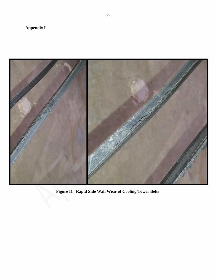
85
Appendix I
Figure I1 –Rapid Side Wall Wear of Cooling Tower Belts
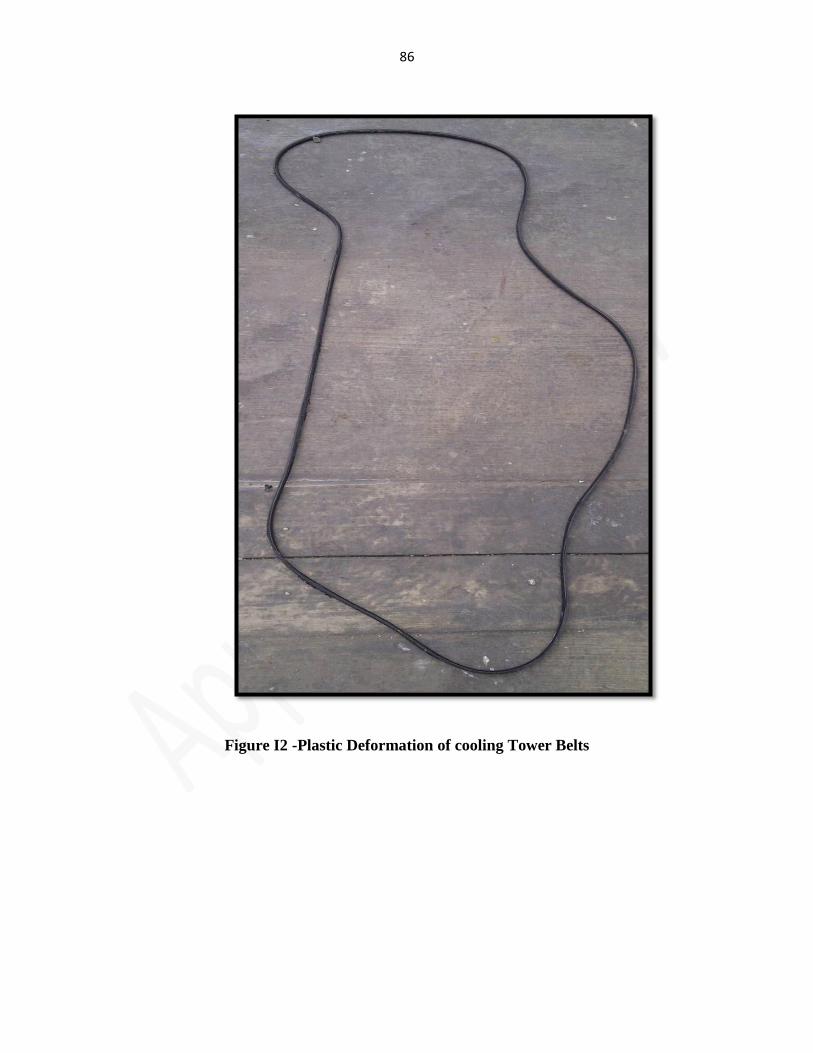
86
Figure I2 -Plastic Deformation of cooling Tower Belts
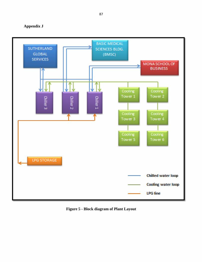
87
Appendix J
Figure 5 - Block diagram of Plant Layout
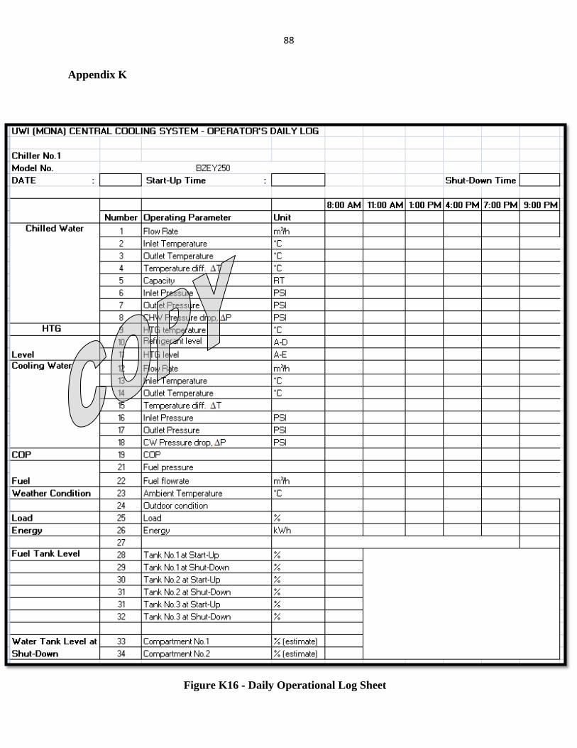
88
Appendix K
Figure K16 - Daily Operational Log Sheet

89
Utrameter
Infrared Thermometer
Figure K2 - Ultrameter used at the plant to measure
water parameters
Figure K3 7 - Infrared thermometer used to verify
operating temperature
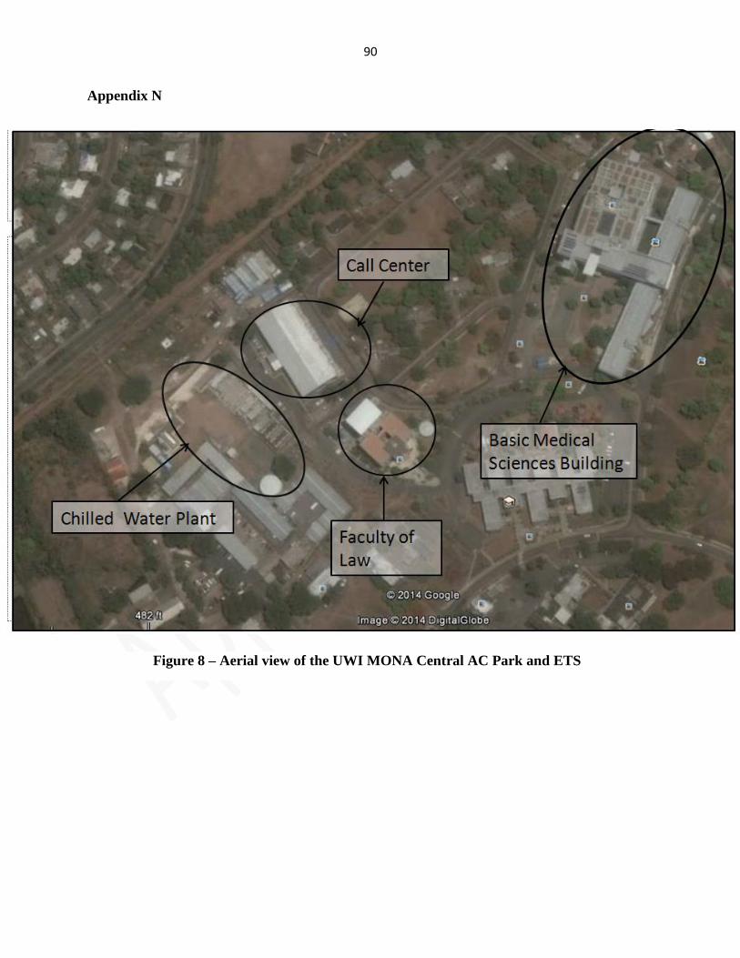
90
Appendix N
Figure 8 – Aerial view of the UWI MONA Central AC Park and ETS
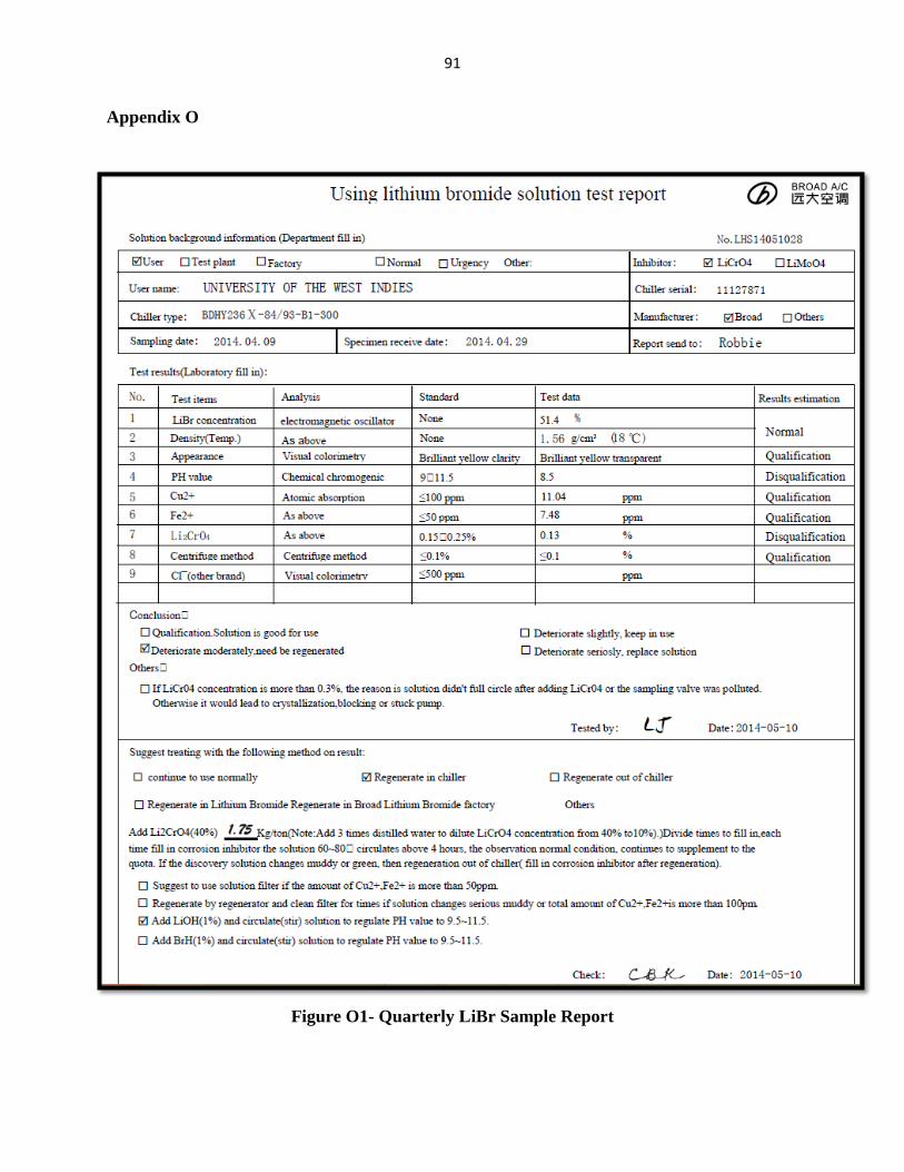
91
Appendix O
Figure O1- Quarterly LiBr Sample Report
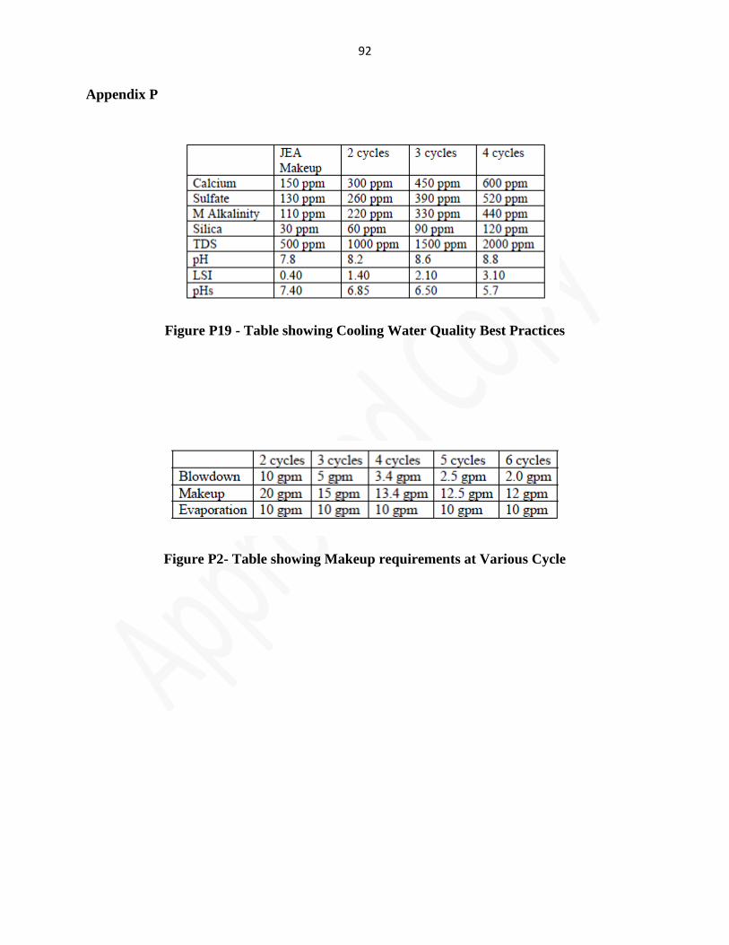
92
Appendix P
Figure P19 - Table showing Cooling Water Quality Best Practices
Figure P2- Table showing Makeup requirements at Various Cycle