Embed Size (px)
Citation preview
Insurance: Mathematics and Economics 26 (2000) 37–57
Fair valuation of life insurance liabilities: The impact of interest rateguarantees, surrender options, and bonus policies
Anders Grosena,1, Peter Løchte Jørgensenb,∗a Department of Finance, Aarhus School of Business, DK-8210 Aarhus V, Denmark
b Department of Management, University of Aarhus, Bldg. 350, DK-8000 Aarhus C, Denmark
Received April 1999; received in revised form August 1999
Abstract
The paper analyzes one of the most common life insurance products — the so-calledparticipating(or with profits) policy.This type of contract stands in contrast to unit-linked (UL) products in that interest is credited to the policy periodicallyaccording to some mechanism which smoothes past returns on the life insurance company’s (LIC) assets. As is the case forUL products, the participating policies are typically equipped with an interest rate guarantee and possibly also an option tosurrender (sell-back) the policy to the LIC before maturity.
The paper shows that the typical participating policy can be decomposed into a risk free bond element, a bonus option, anda surrender option. A dynamic model is constructed in which these elements can be valued separately using contingent claimsanalysis. The impact of various bonus policies and various levels of the guaranteed interest rate is analyzed numerically. Wefind that values of participating policies are highly sensitive to the bonus policy, that surrender options can be quite valuable,and that LIC solvency can be quickly jeopardized if earning opportunities deteriorate in a situation where bonus reserves arelow and promised returns are high. ©2000 Elsevier Science B.V. All rights reserved.
MSC:IM10; IE01. KWD Participating Life Insurance Policies; Embedded options; Contingent claims valuation; Bonus policy; Surrender
JEL classification:G13; G22; G23
1. Introduction
Embedded options pervade the wide range of products offered by pension funds and life insurance companies.Interest rate guarantees, bonus distribution schemes, and surrender possibilities are common examples of implicitoption elements in standard type policies issued in the United States, Europe, as well as in Japan. Such issuedguarantees and written options are liabilities to the issuer. They represent a value and constitute a potential hazard tocompany solvency and these contract elements should therefore ideally be properly valued and reported separately
∗ Corresponding author. Tel.:+45-8942-1544; fax:+45-8613-5132.E-mail addresses:[email protected] (A. Grosen), [email protected] (P. Løchte Jørgensen).
1 Tel.: +45-8948-6427; fax:+45-8615-1943.
0167-6687/00/$ – see front matter ©2000 Elsevier Science B.V. All rights reserved.PII: S0167-6687(99)00041-4
38 A. Grosen, P. Løchte Jørgensen / Insurance: Mathematics and Economics 26 (2000) 37–57
on the liability side of the balance sheet. But historically this has not been done, to which there are a numberof possible explanations. Firstly, it is likely that some companies have failed to realize that their policies in factcomprised multiple components, some of which were shorted options. Secondly, it seems fair to speculate thatother companies have simply not cared. The options embedded in their policies may have appeared sofar out ofthe money, in particular at the time of issuance, that company actuaries have considered the costs associated withproper assessment of their otherwise negligible value to far outweigh any benefits. Thirdly, the lack of analyticaltools for the evaluation of these particular obligations may have played a part. Whatever the reason, we nowknow that the negligence turned out to be catastrophic for some companies, and as a result shareholders andpolicyowners have suffered. In the United States, a large number of companies have been unable to meet theirobligations and have simply defaulted (see e.g. Briys and de Varenne, 1997 and the references cited therein fordetails), whereas in e.g. the United Kingdom and Denmark, companies have started cutting their bonuses in orderto ensure survival.
The main trigger for these unfortunate events is found on the other side of the balance sheet where life insurancecompanies have experienced significantly lower rates of return on their assets than in the 1970s and 1980s. Thelower asset returns in combination with the reluctance of insurance and pension companies to adjust their interestrate guarantees on new policies according to prevailing market conditions have resulted in a dramatic narrowing ofthe safety margin between the companies’ earning power and the level of the promised returns. Stated differently,the issued interest rate guarantees have moved from being far out of the money to being very muchin the money,and many companies have experienced solvency problems as a result. The reality of this threat has most recentlybeen illustrated in Japan where Nissan Mutual life insurance group collapsed as the company failed to meet interestrate guarantees of 4.7% p.a.2 Nissan Mutual’s uncovered liabilities were estimated to amount to $2.56 billion,so in this case policyholders’ options indeed expired in the money without the company being able to fulfil itsobligations.
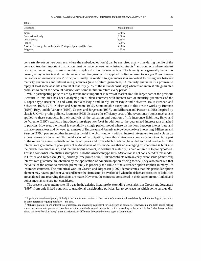
Partly as a result of Nissan Mutual Life’s collapse, Japanese life insurance companies have been ordered toreduce the interest rate guarantee from 4.5% to 2.5% p.a. In Europe, the EU authorities have also responded tothe threat of insolvency from return guarantees. Specifically, Article 18 of the Third EU Life Insurance Directive,which was effective as of 10 November, 1992, requires that interest rate guarantees do not exceed 60% of the rateof return on government debt (of unspecified maturity). In relation to this, Table 1 shows the prevalent maximumlevel of interest rate guarantees as of October 1998 for Japan and the EU member countries. In several of thesecountries, the maximum guaranteed interest rate has decreased during recent years and further cuts are likely to beseen.3
As a consequence of the problems outlined above, insurance companies have experienced an increased focuson their risk management policy from regulatory authorities, academics, and the financial press. In particularthe shortcomings of traditional deterministic actuarial pricing principles when it comes to the valuation of optionelements are surfacing. Recent years have also revealed an increasing interest in applying financial pricing techniquesto the fair valuation of insurance liabilities, see for example Babbel and Merrill (1999), Boyle and Hardy (1997),Vanderhoof and Altman (1998).4
In the literature dealing with the valuation of and to some extent also the reserving for insurance liabilities, severaltypes of contracts and associated guarantees and option elements are recognized. Some of the contracts consideredcontain option elements ofEuropean type, meaning that the option(s) can be exercised only at maturity. This
2 The Financial Times,2 June, 1997.3 From personal communication with members of the Insurance Committee ofGroupe Consultatif des Associations d’Actuaires des Pays des
Communautes Europeennes(sic!).4 The concern about traditional deterministic actuarial pricing principles and in particular theprinciple of equivalenceis not entirely new. In
the United Kingdom, the valuation ofmaturity guarantees(as opposed to theinterest rate guaranteesstudied in the present paper) was a concern20 years ago when the Institute of Actuaries commissioned the Report of the Maturity Guarantees Working Party (1980), in which the valuationof maturity guarantees in life insurance was studied (see also the discussion in Boyle and Hardy, 1997). It was recognized that a guarantee hasa cost and that explicit payment for these guarantees is necessary. For an interesting view and a discussion of actuarial vs. financial pricing, thereader is referred to Embrechts (1996).
A. Grosen, P. Løchte Jørgensen / Insurance: Mathematics and Economics 26 (2000) 37–57 39
Table 1
Countries Maximum rate
Japan 2.50%Denmark and Italy 3.00%Luxembourg 3.50%France 3.75%Austria, Germany, the Netherlands, Portugal, Spain, and Sweden 4.00%Belgium 4.75%
contrastsAmerican typecontracts where the embedded option(s) can be exercised at any time during the life of thecontract. Another important distinction must be made between unit-linked contracts5 and contracts where interestis credited according to some smoothing surplus distribution mechanism. The latter type is generally known asparticipatingcontracts and the interest rate crediting mechanism applied is often referred to as aportfolio averagemethodor anaverage interest principle. Finally, in relation to guarantees it is important to distinguish betweenmaturity guarantees and interest rate guarantees (rate of return guarantees). A maturity guarantee is a promise torepay at least some absolute amount at maturity (75% of the initial deposit, say) whereas an interest rate guaranteepromises to credit the account balance with some minimum return every period.6
While participating policies are by far the most important in terms of market size, the larger part of the previousliterature in this area has been analyzing unit-linked contracts with interest rate or maturity guarantees of theEuropean type (Baccinello and Ortu, 1993a,b; Boyle and Hardy, 1997; Boyle and Schwartz, 1977; Brennan andSchwartz, 1976, 1979; Nielsen and Sandmann, 1995). Some notable exceptions to this are the works by Brennan(1993), Briys and de Varenne (1997), Grosen and Jørgensen (1997), and Miltersen and Persson (1998). Inspired byclassic UK with profits policies, Brennan (1993) discusses the efficiency costs of the reversionary bonus mechanismapplied to these contracts. In their analysis of the valuation and duration of life insurance liabilities, Briys andde Varenne (1997) explicitly introduce aparticipation levelin addition to the guaranteed interest rate attachedto policies. However, the model is essentially a single period model where distinctions between interest rate andmaturity guarantees and between guarantees of European and American type become less interesting. Miltersen andPersson (1998) present another interesting model in which contracts with an interest rate guarantee and a claim onexcess returns can be valued. To model a kind of participation, the authors introduce a bonus account to which a partof the return on assets is distributed in ‘good’ years and from which funds can be withdrawn and used to fulfil theinterest rate guarantee in poor years. The drawbacks of this model are that no averaging or smoothing is built intothe distribution mechanism, and that the bonus account, if positive at maturity, is paid out in full to policyholders.This is a somewhat unrealistic assumption. Also the American typesurrender optionis not considered in this model.In Grosen and Jørgensen (1997), arbitrage-free prices of unit-linked contracts with an early exercisable (American)interest rate guarantee are obtained by the application of American option pricing theory. They also point out thatthe value of the option to exercise prematurely is precisely the value of the surrender option implicit in many lifeinsurance contracts. The numerical work in Grosen and Jørgensen (1997) demonstrates that this particular optionelement may have significant value and hence that it must not be overlooked when the risk characteristics of liabilitiesare analyzed and reserving decisions are made. However, the contracts considered in their paper are unit-linked andbonus mechanisms are not considered.
The present paper attempts to fill a gap in the existing literature by extending the analysis in Grosen and Jørgensen(1997) from unit-linked contracts to traditional participating policies, i.e. to contracts in which some surplus dis-
5 A policy is unit-linked (equity-linked) if the interest rate credited to the customer’s account is linked directly and without lags to the returnon some reference (equity) portfolio — theunit.
6 Maturity guarantees and interest rate guarantees are obviously equivalent for single period contracts. However, in a multiple period settingwhere the interest rate guarantee is on the current account balance and interest is credited according to the principle that “what has once beengiven, can never be taken away” there is a significant difference between these two types of guarantees.
40 A. Grosen, P. Løchte Jørgensen / Insurance: Mathematics and Economics 26 (2000) 37–57
tribution mechanism is employed each period to credit interest at or above the guaranteed rate. The objective isthus to specify a model which encompasses the common characteristics of life insurance contracts discussed aboveand which can be used for valuation and risk analysis in relation to these particular liabilities. Our work towardsthis goal will meet a chain of distinct challenges: First, asset returns must be credibly modeled. In this respect wetake a completely non-controversial approach and adopt the widely used framework of Black and Scholes (1973).Second, and more importantly, a realistic model for bonus distribution must be specified in a way that integrates theinterest rate guarantee. This is where our main contributions lie. The third challenge is primarily of technical natureand concerns the arbitrage-free valuation of the highly path-dependent contract pay-offs resulting from applyingthe particular bonus distribution mechanism suggested to customer accounts. We will carefully take interest rateguarantees as well as possible surrender options into account and during the course of the analysis we also brieflytouch upon the associated problem of reserving for the liabilities. Finally, we provide a variety of illustrative exam-ples. The numerical section of the paper also contains some insights into the effective implementation of numericalalgorithms for solving the model.
The paper is organized as follows. Section 2 describes the products which will be analyzed and presents the basicmodeling framework. In particular, the bonus policy and the dynamics of assets and liabilities are discussed. InSection 3 we present the methodology applied for contract valuation, we demonstrate how contract values can beconveniently decomposed into their basic elements, and computational aspects are addressed. Numerical results arepresented in Section 4, and Section 5 concludes the paper.
2. The model
In this section we provide a more detailed description of the life insurance contracts and pension plan productswhich we will analyze. Furthermore, we introduce the basic model to be used in the analysis and valuation of thesecontracts, especially the valuation of various embedded option elements.
The basic framework is as follows. Agents are assumed to operate in a continuous time frictionless economy witha perfect financial market, so that tax effects, transaction costs, divisibility, liquidity, and short-sales constraints andother imperfections can be ignored. As regards the specific contracts, we also ignore the effects of expense charges,lapses and mortality.7
At time zero (the beginning of year one) thepolicyholdermakes a single-sum deposit,V0, with the insur-ance company. 8 He thereby acquires apolicy or a contract of nominal valueP0 which we will treat as a fi-nancial asset, or more precisely, as a contingent claim. In general, we will treatP0 as being exogenous whereasthe fair value of the contract,V0, is to be determined.V0 may be smaller or larger thanP0 depending on thecontractual terms, particularly the various option elements. The policy matures afterT years when the accountis settled by a single payment from the insurance company to the policyholder. However, in some cases tobe further discussed below, we will allow the policy to be terminated at the policyholder’s discretion prior totimeT.
At the inception of the contract, the insurance company invests the trusted funds in the financial market andcommits to crediting interest on the policy’s account balance according to some pay-out scheme linked to eachyear’s market return until the contract expires. We will discuss the terms for the market investment and the exactnature of thisinterest rate crediting mechanismin more detail shortly. For now we merely note that the interest
7 Since we ignore the insurance aspects mentioned and focus entirely on financial risks, the reader may also simply think of the products analyzedas a specific form ofguaranteed investment contracts(GICs). In general, GICs in their various forms have been a significant investment vehiclefor pension plans over the last 20 years. In the early 1990s, confidence in GICs was seriously shaken by the financial troubles of some insurancecompanies that were affected by defaults of junk bonds they purchased in the 1980s and poor mortgage loan results. GICs do not generally enjoythe status of ‘insurance’, and therefore they are not entitled to state guarantee fund coverage in the event of defaults (Black and Skipper, 1994,pp. 814–815.)
8 The extension to periodic premiums is straightforward, but omitted owing to space considerations.
A. Grosen, P. Løchte Jørgensen / Insurance: Mathematics and Economics 26 (2000) 37–57 41
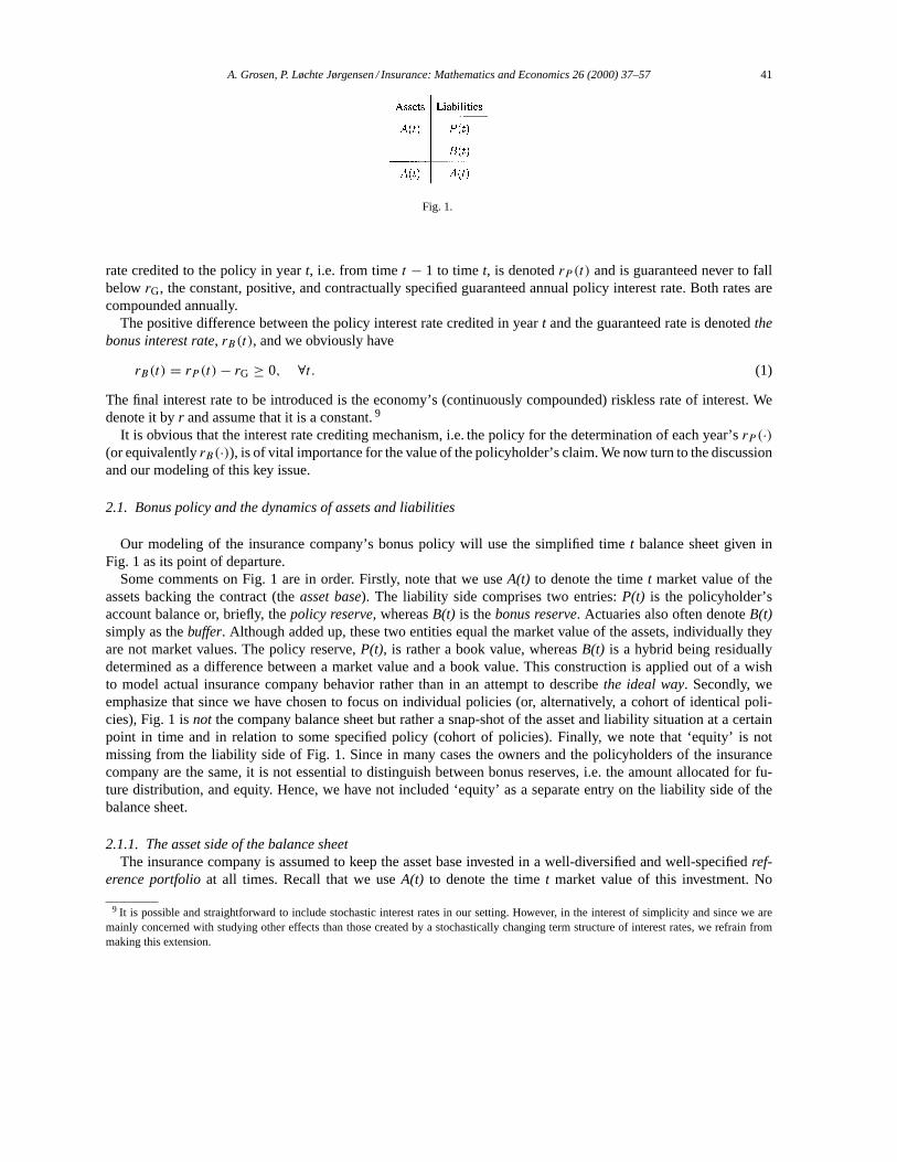
Fig. 1.
rate credited to the policy in yeart, i.e. from timet − 1 to timet, is denotedrP (t) and is guaranteed never to fallbelowrG, the constant, positive, and contractually specified guaranteed annual policy interest rate. Both rates arecompounded annually.
The positive difference between the policy interest rate credited in yeart and the guaranteed rate is denotedthebonus interest rate, rB(t), and we obviously have
rB(t) = rP (t) − rG ≥ 0, ∀t. (1)
The final interest rate to be introduced is the economy’s (continuously compounded) riskless rate of interest. Wedenote it byr and assume that it is a constant.9
It is obvious that the interest rate crediting mechanism, i.e. the policy for the determination of each year’srP (·)(or equivalentlyrB(·)), is of vital importance for the value of the policyholder’s claim. We now turn to the discussionand our modeling of this key issue.
2.1. Bonus policy and the dynamics of assets and liabilities
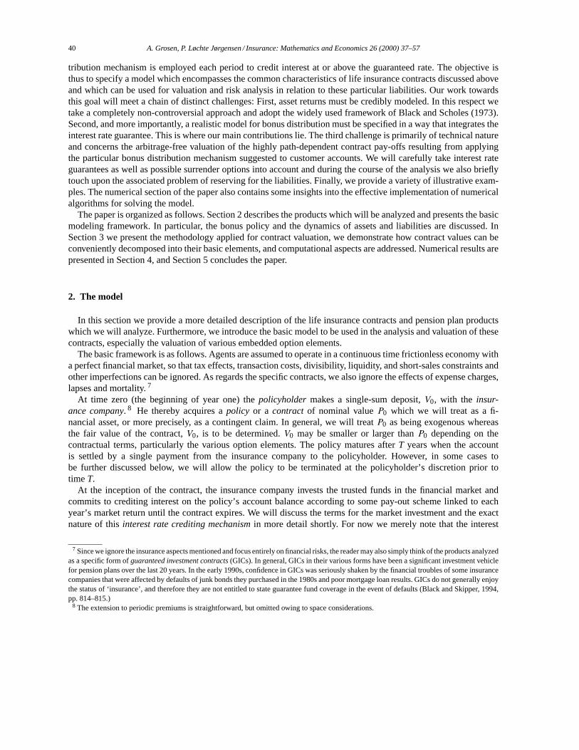
Our modeling of the insurance company’s bonus policy will use the simplified timet balance sheet given inFig. 1 as its point of departure.
Some comments on Fig. 1 are in order. Firstly, note that we useA(t) to denote the timet market value of theassets backing the contract (theasset base). The liability side comprises two entries:P(t) is the policyholder’saccount balance or, briefly, thepolicy reserve, whereasB(t) is thebonus reserve. Actuaries also often denoteB(t)simply as thebuffer. Although added up, these two entities equal the market value of the assets, individually theyare not market values. The policy reserve,P(t), is rather a book value, whereasB(t) is a hybrid being residuallydetermined as a difference between a market value and a book value. This construction is applied out of a wishto model actual insurance company behavior rather than in an attempt to describethe ideal way. Secondly, weemphasize that since we have chosen to focus on individual policies (or, alternatively, a cohort of identical poli-cies), Fig. 1 isnot the company balance sheet but rather a snap-shot of the asset and liability situation at a certainpoint in time and in relation to some specified policy (cohort of policies). Finally, we note that ‘equity’ is notmissing from the liability side of Fig. 1. Since in many cases the owners and the policyholders of the insurancecompany are the same, it is not essential to distinguish between bonus reserves, i.e. the amount allocated for fu-ture distribution, and equity. Hence, we have not included ‘equity’ as a separate entry on the liability side of thebalance sheet.
2.1.1. The asset side of the balance sheetThe insurance company is assumed to keep the asset base invested in a well-diversified and well-specifiedref-
erence portfolioat all times. Recall that we useA(t) to denote the timet market value of this investment. No
9 It is possible and straightforward to include stochastic interest rates in our setting. However, in the interest of simplicity and since we aremainly concerned with studying other effects than those created by a stochastically changing term structure of interest rates, we refrain frommaking this extension.
42 A. Grosen, P. Løchte Jørgensen / Insurance: Mathematics and Economics 26 (2000) 37–57
assumptions are made regarding the composition of this portfolio with respect to equities, bonds, real estate, orregarding the dynamics of its individual elements. We simply work on an aggregate level and assume that the totalmarket value evolves according to a geometric Brownian motion,10
dA(t) = µA(t)dt + σA(t) dW(t), A(0) = A0. (2)
Hereµ, σ , andA0 are constants andW(·) is a standard Brownian motion defined on the filtered probability space(�,F, (Ft ), P ) on the finite interval [0, T ]. 11
For the remaining part of the paper we shall work under the familiar equivalent risk neutral probability mea-sure,Q (see e.g. Harrison and Kreps, 1979) under which discounted prices areQ-martingales and where wehave
dA(t) = rA(t)dt + σA(t)dWQ(t), A(0) = A0, (3)
and whereWQ(·) is a standard Brownian motion underQ. The stochastic differential equation in (3) has a well-knownsolution given by
A(t) = A0 · e(r−(1/2)σ2)t+σWQ(t). (4)
In particular, we will need to work with annual (log) returns which are easily established as conditionally normal:
ln A(t)/A(t − 1)|Ft−1 = r − 12σ 2 + σ
(WQ(t) − WQ(t − 1)
)|Ft−1 ∼ N
(r − 1
2σ 2, σ 2)
. (5)
2.1.2. The liability side of the balance sheetWe now direct our attention towards describing the dynamics of the liability side of the balance sheet. Referring
to Fig. 1, we have previously introduced the two entriesP(t) andB(t) as the policy reserve and the bonus reserve,or alternatively, as the policyholder’s account balance and the buffer. Regardless of terminology, it is important notto confuseP(t) with the concurrent fair value of the policy.
The distribution of funds to the two liability entries over time is determined by the bonus policy, i.e. by thesequencerP (t) for t ∈ ϒ ≡ {1, 2, . . . , T }. In particular, note that from the earlier definition of the policy interestrate we must have
P(t) = (1 + rP (t)) · P(t − 1), t ∈ ϒ, (6)
from which we deduce
P(t) = P0
t∏i=1
(1 + rP (i)), t ∈ ϒ. (7)
These are obviously two rather empty expressions until we know more about the determinants of the processfollowed byrP (·), i.e. the interest rate crediting mechanism. Not until more has been said about this issue can we
10 The assumption that assets evolve according to the GBM is not motivated by a wish to obtainclosed formor analytic solutions to the problemsstudied. Indeed, due to the complexity of the contract pay-offs, we obtain no such solutions and we resort instead to extensive use of numericalmethods. The numerical analysis could just as easily be carried out using another model for the evolution in asset values. Actuaries, for example,may prefer to apply the Wilkie model to describe the evolution of asset values (see e.g. Boyle and Hardy, 1997). Another interesting possibilityis to let assets evolve according to a jump-diffusion model.11 The assumption thatµ is constant is made for simplicity and is a bit stronger than necessary. As pointed out by Black and Scholes (1973),standard arbitrage valuation carries through without changes if we allowµ to depend on time and/or the current state.
A. Grosen, P. Løchte Jørgensen / Insurance: Mathematics and Economics 26 (2000) 37–57 43
start to study the dynamics of the liability side of the balance sheet (in particular the policyholder’s account) andthe valuation of the policyholder’s contract.
The question of howrP (·) is determined in practice is highly subtle involving intangible political, legal, andstrategic considerations within the insurance company. There is therefore little hope that we can ever constructsimple models which canpreciselycapture all elements of this process. In particular, the theoretical possibility forthe management of the insurance company to change the surplus distribution policy over time — perhaps withinspecific limits set by law — will be problematic for the task of valuing the policyholder’s claim. Put differently,this means that whenever we apply and analyze a certain interest rate crediting mechanism in our models, weshould keep in mind that we are not necessarily dealing with strictly (legally) binding agreements between theparties.
Having realized these problems — of which we are unaware of parallels in the standard financial (exotic) optionsliterature — we will proceed with an attempt to specify an interest rate crediting mechanism which is as accurate andrealistic an approximation to the true bonus policy as possible. We shall specify the interest rate crediting mechanismin the form of a mathematically well-defined function in order to be able to apply the powerful apparatus of financialmathematics and, in particular, arbitrage pricing.
While problemsdo exist as outlined above, there are fortunately also some well-established principles that canbe used as inspiration. Firstly, it is clear that realized returns on the assets in a given year must influence the policyinterest rate in the ensuing year(s). Secondly, since one of the main arguments in the marketing of these life insurancepolicies is that they provide a low-risk, stable, and yet competitive return compared with other marketed assets,our modeling of the interest rate crediting mechanism should also accomplish this. The surplus distribution ruleshould in other words resemble what is known in the industry as the average interest principle.12 Thirdly, in orderto provide these stable returns to policyholders13 and to partially protect themselves against insolvency, the lifeinsurance companies aim at building and maintaining a certain level of reserves (the buffer). This could and shouldalso be accounted for in constructing the distribution rule.
In sum, an attempt to model actual interest rate crediting behavior of life insurance companies should involvethe specification of a functional relationship from the asset base,A(·), and the bonus reserve,B(·), to the policyinterest rate,rP (t). In this way, the annual interest bonus can be based on the actual investment performance aswell as on the current financial position (the degree of solvency) of the life insurance company. Furthermore, thefunctional relationship should be constructed in such a way that policy interest rates are in effect low-volatility,smoothed market returns.
We thus propose to proceed in the following way. It is first assumed that the insurance company’s managementhas specified a constant target for the ratio of bonus reserves to policy reserves, i.e. the ratioB(t)/P (t). We callthis thetarget buffer ratioand denote it byγ . A realistic value would be in the order of 10–15%. Suppose furtherthat it is the insurance company’s objective to distribute to policyholders’ accounts a positive fraction,α, of anyexcessive bonus reserve in each period. The company must, however, always credit at least the guaranteed rate,rG, which it will do if the bonus reserve is insufficient or even negative. Clearly for appropriate values ofα thismechanism will ensure a stable smoothing of the surplus. The coefficientα is referred to as thedistribution ratio. 14
A realistic value ofα is in the area of 20–30%. Before we proceed, let us briefly recapitulate the most frequentlyapplied notation:
12 The average interest principle is discussed in e.g. Nielsen and Thaning (1996). These authors write
“... the average interest principle used by most of the pension business, partly to assure the customer a positive yield each year and partlyto minimize the companies’ risk due to the interest guarantee given — means that the yield given to the insured is very different from thecompanies’ yield on investments each year. The difference is regulated by the so-called dividend equalization provisions.”
13 Insurance companies sometimes label their bonus reserves ‘bonus smoothing reserves’ indicating their role in sustaining the average interestprinciple.14 Briys and de Varenne (1997) work with a similar parameter called theparticipation coefficient.

44 A. Grosen, P. Løchte Jørgensen / Insurance: Mathematics and Economics 26 (2000) 37–57
P0 policy account balance at time 0T maturity date of the contractrP (t) policy interest rate in yeartrG guaranteed interest raterB(t) bonus interest rate in yeart
r riskless interest rateA(t) market value of insurance company’s assets at timet
P (t) policy reserve at timetB(t) bonus reserve at timetγ target buffer ratioα distribution ratioσ asset volatility
(8)
The discussion above can now be formalized by setting up the following analytical scheme for the interest ratecredited to policyholders’ accounts in yeart ,
rP (t) = max
{rG, α
(B(t − 1)
P (t − 1)− γ
)}. (9)
This implies a bonus interest rate as stated below,
rB(t) = max
{0, α
(B(t − 1)
P (t − 1)− γ
)− rG
}. (10)
Note first that as in real life contracts, the interest rate credited between timet − 1 and timet is determined at timet − 1, i.e. there is a degree of predictability in the interest rate crediting mechanism.15 Observe also that whenrG < α((B(t − 1)/P (t − 1)) − γ ) (reserves are ‘high’) we can write
P(t) = P(t − 1)
(1 + α
(B(t − 1)
P (t − 1)− γ
))= P(t − 1) + α (B(t − 1) − γP (t − 1))
= P(t − 1) + α(B(t − 1) − B∗(t − 1)
), (11)
whereB∗(t − 1) ≡ γP (t − 1) denotes the optimal reserve at timet − 1. Hence, when reserves are satisfactorilylarge, a fixed fraction of the excessive reserve is distributed to policyholders.16
Returning to the general evolution of the policyholder’s account, we have the relation
P(t) = P(t − 1)
(1 + max
{rG, α
(B(t − 1)
P (t − 1)− γ
)})
= P(t − 1)
(1 + rG + max
{0, α
(A(t − 1) − P(t − 1)
P (t − 1)− γ
)− rG
}). (12)
This difference equation clarifies a couple of points. Firstly, it is seen that the interest rate guarantee implies a floorunder the final payout from the contract. The floor is given asPmin(T ) = (1+ rG)T · P(0) and it becomes effectivein case bonus is never distributed to the policy. But note also that as soon as bonus has been distributed once, the
15 In Denmark, for example, all major insurance companies announce their policy interest rate for the coming year in mid-December the yearbefore.16 Note that if one prefers to use continuously compounded rates throughout, one should use
rP (t) = max
{rG, ln
(1 + α
(B(t − 1)
P (t − 1)− γ
))}
instead of (9) andP(t) = P(t − 1) · erP (t) instead of (6) and so on.
A. Grosen, P. Løchte Jørgensen / Insurance: Mathematics and Economics 26 (2000) 37–57 45
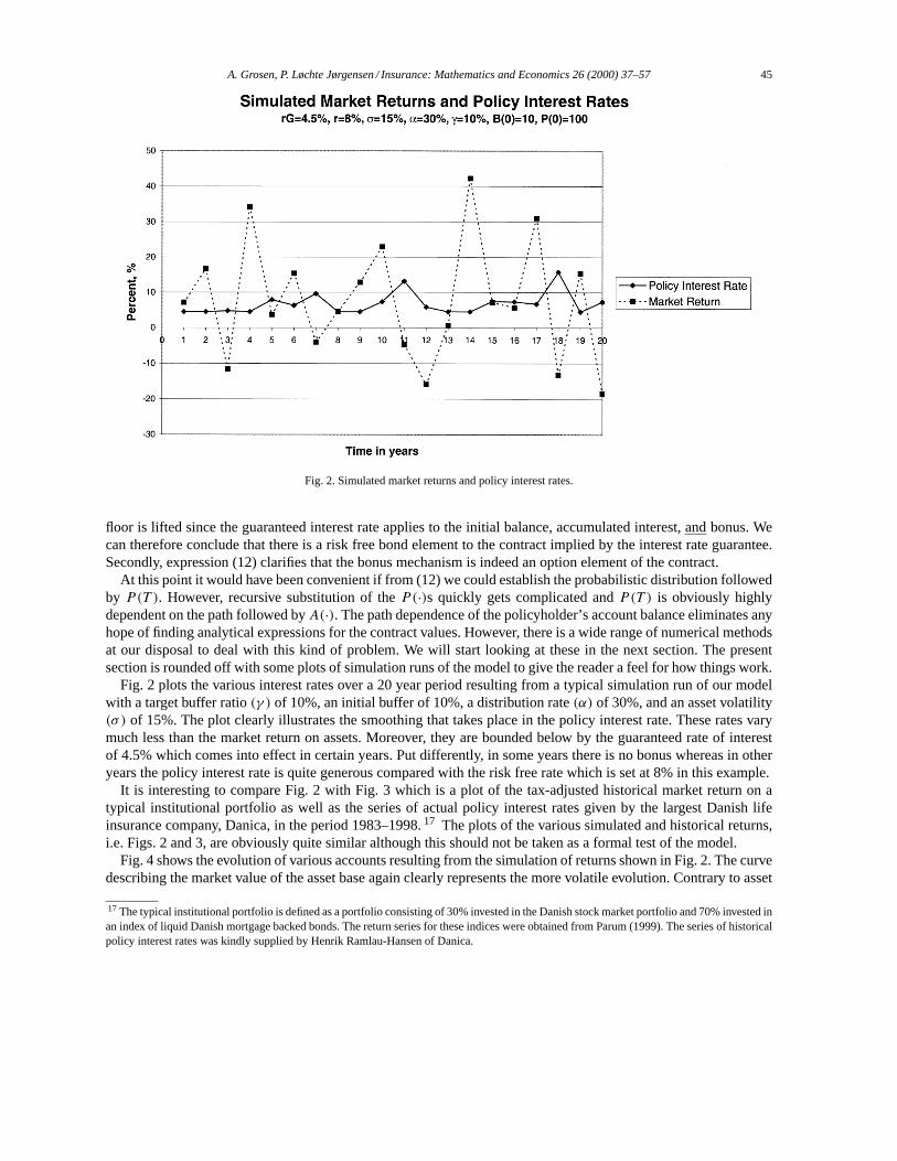
Fig. 2. Simulated market returns and policy interest rates.
floor is lifted since the guaranteed interest rate applies to the initial balance, accumulated interest, andbonus. Wecan therefore conclude that there is a risk free bond element to the contract implied by the interest rate guarantee.Secondly, expression (12) clarifies that the bonus mechanism is indeed an option element of the contract.
At this point it would have been convenient if from (12) we could establish the probabilistic distribution followedby P(T ). However, recursive substitution of theP(·)s quickly gets complicated andP(T ) is obviously highlydependent on the path followed byA(·). The path dependence of the policyholder’s account balance eliminates anyhope of finding analytical expressions for the contract values. However, there is a wide range of numerical methodsat our disposal to deal with this kind of problem. We will start looking at these in the next section. The presentsection is rounded off with some plots of simulation runs of the model to give the reader a feel for how things work.
Fig. 2 plots the various interest rates over a 20 year period resulting from a typical simulation run of our modelwith a target buffer ratio(γ ) of 10%, an initial buffer of 10%, a distribution rate(α) of 30%, and an asset volatility(σ ) of 15%. The plot clearly illustrates the smoothing that takes place in the policy interest rate. These rates varymuch less than the market return on assets. Moreover, they are bounded below by the guaranteed rate of interestof 4.5% which comes into effect in certain years. Put differently, in some years there is no bonus whereas in otheryears the policy interest rate is quite generous compared with the risk free rate which is set at 8% in this example.
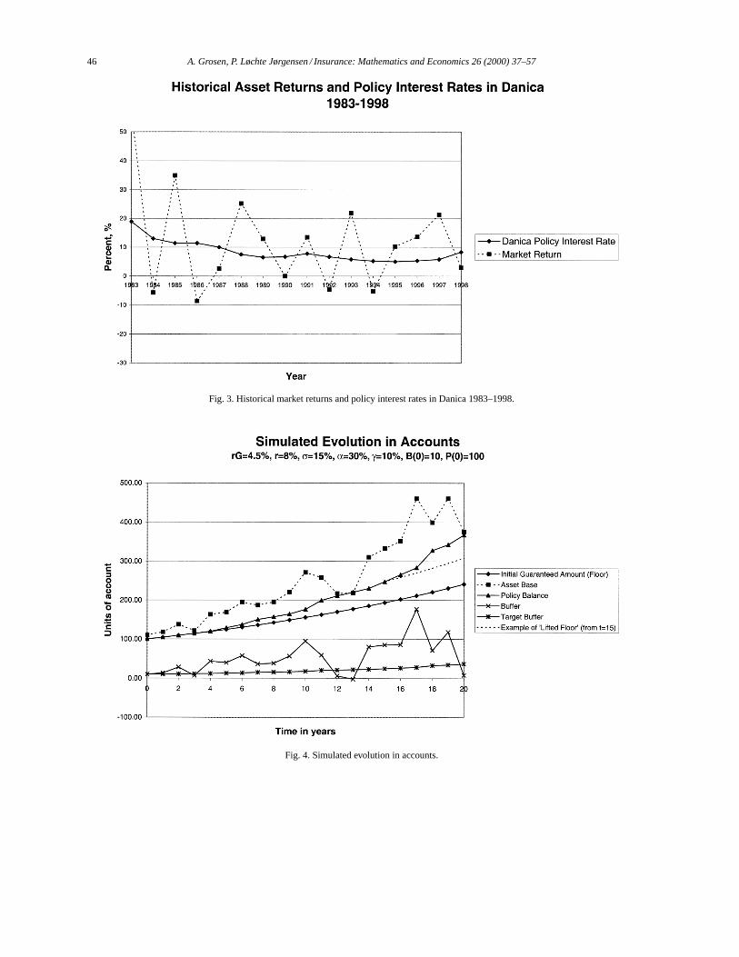
It is interesting to compare Fig. 2 with Fig. 3 which is a plot of the tax-adjusted historical market return on atypical institutional portfolio as well as the series of actual policy interest rates given by the largest Danish lifeinsurance company, Danica, in the period 1983–1998.17 The plots of the various simulated and historical returns,i.e. Figs. 2 and 3, are obviously quite similar although this should not be taken as a formal test of the model.
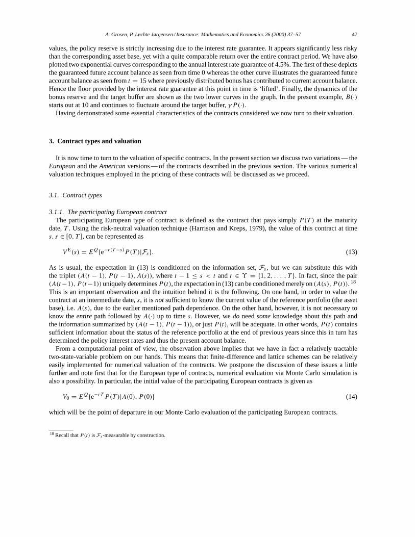
Fig. 4 shows the evolution of various accounts resulting from the simulation of returns shown in Fig. 2. The curvedescribing the market value of the asset base again clearly represents the more volatile evolution. Contrary to asset
17 The typical institutional portfolio is defined as a portfolio consisting of 30% invested in the Danish stock market portfolio and 70% invested inan index of liquid Danish mortgage backed bonds. The return series for these indices were obtained from Parum (1999). The series of historicalpolicy interest rates was kindly supplied by Henrik Ramlau-Hansen of Danica.
46 A. Grosen, P. Løchte Jørgensen / Insurance: Mathematics and Economics 26 (2000) 37–57
Fig. 3. Historical market returns and policy interest rates in Danica 1983–1998.
Fig. 4. Simulated evolution in accounts.
A. Grosen, P. Løchte Jørgensen / Insurance: Mathematics and Economics 26 (2000) 37–57 47
values, the policy reserve is strictly increasing due to the interest rate guarantee. It appears significantly less riskythan the corresponding asset base, yet with a quite comparable return over the entire contract period. We have alsoplotted two exponential curves corresponding to the annual interest rate guarantee of 4.5%. The first of these depictsthe guaranteed future account balance as seen from time 0 whereas the other curve illustrates the guaranteed futureaccount balance as seen fromt = 15 where previously distributed bonus has contributed to current account balance.Hence the floor provided by the interest rate guarantee at this point in time is ‘lifted’. Finally, the dynamics of thebonus reserve and the target buffer are shown as the two lower curves in the graph. In the present example,B(·)starts out at 10 and continues to fluctuate around the target buffer,γP (·).
Having demonstrated some essential characteristics of the contracts considered we now turn to their valuation.
3. Contract types and valuation
It is now time to turn to the valuation of specific contracts. In the present section we discuss two variations — theEuropeanand theAmericanversions — of the contracts described in the previous section. The various numericalvaluation techniques employed in the pricing of these contracts will be discussed as we proceed.
3.1. Contract types
3.1.1. The participating European contractThe participating European type of contract is defined as the contract that pays simplyP(T ) at the maturity
date,T . Using the risk-neutral valuation technique (Harrison and Kreps, 1979), the value of this contract at times, s ∈ [0, T ], can be represented as
V E(s) = EQ{e−r(T −s)P (T )|Fs}. (13)
As is usual, the expectation in (13) is conditioned on the information set,Fs , but we can substitute this withthe triplet(A(t − 1), P (t − 1), A(s)), wheret − 1 ≤ s < t and t ∈ ϒ = {1, 2, . . . , T }. In fact, since the pair(A(t−1), P (t−1)) uniquely determinesP(t), the expectation in (13) can be conditioned merely on(A(s), P (t)). 18
This is an important observation and the intuition behind it is the following. On one hand, in order to value thecontract at an intermediate date,s, it is notsufficient to know the current value of the reference portfolio (the assetbase), i.e.A(s), due to the earlier mentioned path dependence. On the other hand, however, it is not necessary toknow theentire path followed byA(·) up to times. However, wedo needsomeknowledge about this path andthe information summarized by(A(t − 1), P (t − 1)), or justP(t), will be adequate. In other words,P(t) containssufficient information about the status of the reference portfolio at the end of previous years since this in turn hasdetermined the policy interest rates and thus the present account balance.
From a computational point of view, the observation above implies that we have in fact a relatively tractabletwo-state-variable problem on our hands. This means that finite-difference and lattice schemes can be relativelyeasily implemented for numerical valuation of the contracts. We postpone the discussion of these issues a littlefurther and note first that for the European type of contracts, numerical evaluation via Monte Carlo simulation isalso a possibility. In particular, the initial value of the participating European contracts is given as
V0 = EQ{e−rT P (T )|A(0), P (0)} (14)
which will be the point of departure in our Monte Carlo evaluation of the participating European contracts.
18 Recall thatP(t) is Fs -measurable by construction.
48 A. Grosen, P. Løchte Jørgensen / Insurance: Mathematics and Economics 26 (2000) 37–57
Fig. 5.
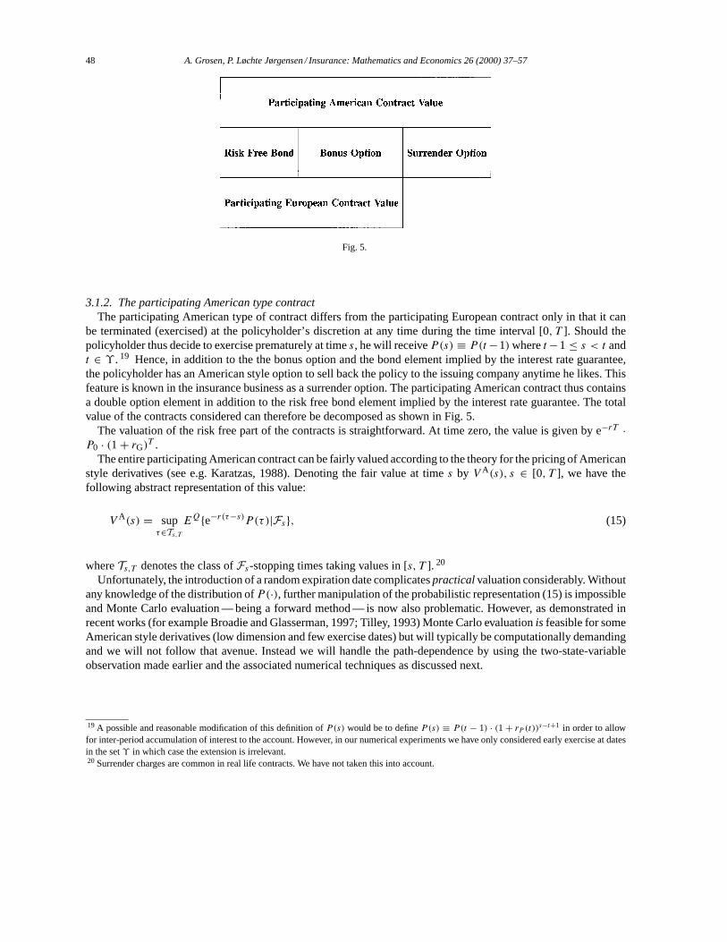
3.1.2. The participating American type contractThe participating American type of contract differs from the participating European contract only in that it can
be terminated (exercised) at the policyholder’s discretion at any time during the time interval [0, T ]. Should thepolicyholder thus decide to exercise prematurely at times, he will receiveP(s) ≡ P(t −1) wheret −1 ≤ s < t andt ∈ ϒ . 19 Hence, in addition to the the bonus option and the bond element implied by the interest rate guarantee,the policyholder has an American style option to sell back the policy to the issuing company anytime he likes. Thisfeature is known in the insurance business as a surrender option. The participating American contract thus containsa double option element in addition to the risk free bond element implied by the interest rate guarantee. The totalvalue of the contracts considered can therefore be decomposed as shown in Fig. 5.
The valuation of the risk free part of the contracts is straightforward. At time zero, the value is given by e−rT ·P0 · (1 + rG)T .
The entire participating American contract can be fairly valued according to the theory for the pricing of Americanstyle derivatives (see e.g. Karatzas, 1988). Denoting the fair value at times by V A(s), s ∈ [0, T ], we have thefollowing abstract representation of this value:
V A(s) = supτ∈Ts,T
EQ{e−r(τ−s)P (τ )|Fs}, (15)
whereTs,T denotes the class ofFs-stopping times taking values in [s, T ]. 20
Unfortunately, the introduction of a random expiration date complicatespracticalvaluation considerably. Withoutany knowledge of the distribution ofP(·), further manipulation of the probabilistic representation (15) is impossibleand Monte Carlo evaluation — being a forward method — is now also problematic. However, as demonstrated inrecent works (for example Broadie and Glasserman, 1997; Tilley, 1993) Monte Carlo evaluationis feasible for someAmerican style derivatives (low dimension and few exercise dates) but will typically be computationally demandingand we will not follow that avenue. Instead we will handle the path-dependence by using the two-state-variableobservation made earlier and the associated numerical techniques as discussed next.
19 A possible and reasonable modification of this definition ofP(s) would be to defineP(s) ≡ P(t − 1) · (1 + rP (t))s−t+1 in order to allowfor inter-period accumulation of interest to the account. However, in our numerical experiments we have only considered early exercise at datesin the setϒ in which case the extension is irrelevant.20 Surrender charges are common in real life contracts. We have not taken this into account.
A. Grosen, P. Løchte Jørgensen / Insurance: Mathematics and Economics 26 (2000) 37–57 49
3.2. Computational aspects
3.2.1. Monte Carlo simulationAs mentioned in the previous section, the participating contracts of European type can be valued by standard
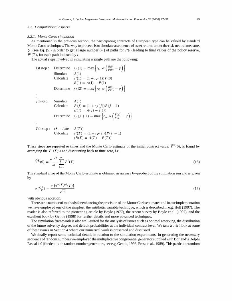
Monte Carlo techniques. The way to proceed is to simulate a sequence of asset returns under the risk-neutral measure,Q, (see Eq. (5)) in order to get a large number (m) of paths forP(·) leading to final values of the policy reserve,P i(T ), for each path indexed byi.
The actual steps involved in simulating a single path are the following:
1st step : Determine rP (1) = max{rG, α
(B(0)P (0)
− γ)}
Simulate A(1)
Calculate P(1) = (1 + rP (1))P (0)
B(1) = A(1) − P(1)
Determine rP (2) = max{rG, α
(B(1)P (1)
− γ)}
...
j th step : Simulate A(j)
Calculate P(j) = (1 + rP (j))P (j − 1)
B(j) = A(j) − P(j)
Determine rP (j + 1) = max{rG, α
(B(j)P (j)
− γ)}
...
T th step : (Simulate A(T ))
Calculate P(T ) = (1 + rP (T ))P (T − 1)
(B(T ) = A(T ) − P(T ))
These steps are repeatedm times and the Monte Carlo estimate of the initial contract value,V E(0), is found byaveraging theP i(T )′s and discounting back to time zero, i.e.
V E(0) = e−rT
m
m∑i=1
P i(T ). (16)
The standard error of the Monte Carlo estimate is obtained as an easy by-product of the simulation run and is givenby
σ(V E0 ) = σ
(e−rT P i(T )
)√
m(17)
with obvious notation.There are a number of methods for enhancing the precision of the Monte Carlo estimates and in our implementation
we have employed one of the simplest, the antithetic variable technique, which is described in e.g. Hull (1997). Thereader is also referred to the pioneering article by Boyle (1977), the recent survey by Boyle et al. (1997), and theexcellent book by Gentle (1998) for further details and more advanced techniques.
The simulation framework is also well-suited for the analysis of issues such as optimal reserving, the distributionof the future solvency degree, and default probabilities at the individual contract level. We take a brief look at someof these issues in Section 4 where our numerical work is presented and discussed.
We finally report some technical details in relation to the simulation experiments. In generating the necessarysequence of random numbers we employed the multiplicative congruential generator supplied with Borland’s DelphiPascal 4.0 (for details on random number generators, see e.g. Gentle, 1998; Press et al., 1989). This particular random
50 A. Grosen, P. Løchte Jørgensen / Insurance: Mathematics and Economics 26 (2000) 37–57
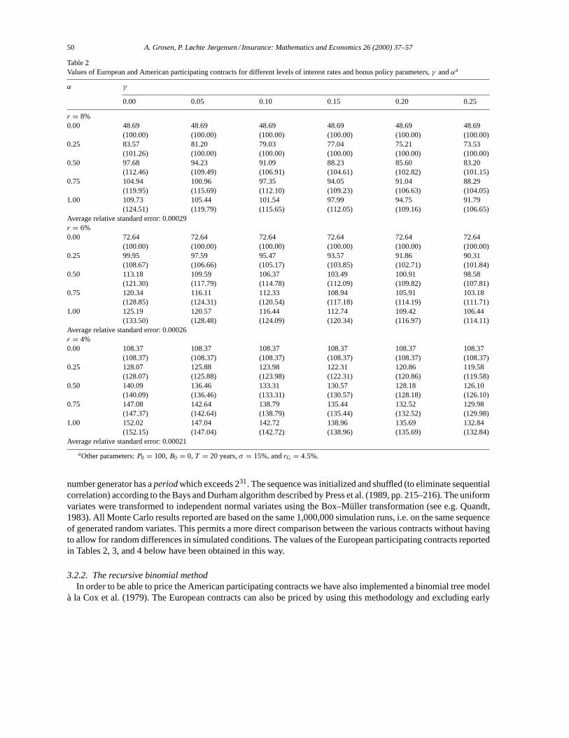
Table 2Values of European and American participating contracts for different levels of interest rates and bonus policy parameters,γ andαa
α γ
0.00 0.05 0.10 0.15 0.20 0.25
r = 8%0.00 48.69 48.69 48.69 48.69 48.69 48.69
(100.00) (100.00) (100.00) (100.00) (100.00) (100.00)0.25 83.57 81.20 79.03 77.04 75.21 73.53
(101.26) (100.00) (100.00) (100.00) (100.00) (100.00)0.50 97.68 94.23 91.09 88.23 85.60 83.20
(112.46) (109.49) (106.91) (104.61) (102.82) (101.15)0.75 104.94 100.96 97.35 94.05 91.04 88.29
(119.95) (115.69) (112.10) (109.23) (106.63) (104.05)1.00 109.73 105.44 101.54 97.99 94.75 91.79
(124.51) (119.79) (115.65) (112.05) (109.16) (106.65)Average relative standard error: 0.00029r = 6%0.00 72.64 72.64 72.64 72.64 72.64 72.64
(100.00) (100.00) (100.00) (100.00) (100.00) (100.00)0.25 99.95 97.59 95.47 93.57 91.86 90.31
(108.67) (106.66) (105.17) (103.85) (102.71) (101.84)0.50 113.18 109.59 106.37 103.49 100.91 98.58
(121.30) (117.79) (114.78) (112.09) (109.82) (107.81)0.75 120.34 116.11 112.33 108.94 105.91 103.18
(128.85) (124.31) (120.54) (117.18) (114.19) (111.71)1.00 125.19 120.57 116.44 112.74 109.42 106.44
(133.50) (128.48) (124.09) (120.34) (116.97) (114.11)Average relative standard error: 0.00026r = 4%0.00 108.37 108.37 108.37 108.37 108.37 108.37
(108.37) (108.37) (108.37) (108.37) (108.37) (108.37)0.25 128.07 125.88 123.98 122.31 120.86 119.58
(128.07) (125.88) (123.98) (122.31) (120.86) (119.58)0.50 140.09 136.46 133.31 130.57 128.18 126.10
(140.09) (136.46) (133.31) (130.57) (128.18) (126.10)0.75 147.08 142.64 138.79 135.44 132.52 129.98
(147.37) (142.64) (138.79) (135.44) (132.52) (129.98)1.00 152.02 147.04 142.72 138.96 135.69 132.84
(152.15) (147.04) (142.72) (138.96) (135.69) (132.84)Average relative standard error: 0.00021
aOther parameters:P0 = 100,B0 = 0, T = 20 years,σ = 15%, andrG = 4.5%.
number generator has aperiodwhich exceeds 231. The sequence was initialized and shuffled (to eliminate sequentialcorrelation) according to the Bays and Durham algorithm described by Press et al. (1989, pp. 215–216). The uniformvariates were transformed to independent normal variates using the Box–Müller transformation (see e.g. Quandt,1983). All Monte Carlo results reported are based on the same 1,000,000 simulation runs, i.e. on the same sequenceof generated random variates. This permits a more direct comparison between the various contracts without havingto allow for random differences in simulated conditions. The values of the European participating contracts reportedin Tables 2, 3, and 4 below have been obtained in this way.
3.2.2. The recursive binomial methodIn order to be able to price the American participating contracts we have also implemented a binomial tree model
à la Cox et al. (1979). The European contracts can also be priced by using this methodology and excluding early
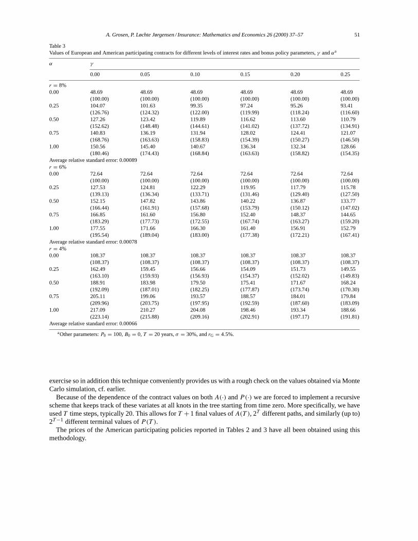
A. Grosen, P. Løchte Jørgensen / Insurance: Mathematics and Economics 26 (2000) 37–57 51
Table 3Values of European and American participating contracts for different levels of interest rates and bonus policy parameters,γ andαa
α γ
0.00 0.05 0.10 0.15 0.20 0.25
r = 8%0.00 48.69 48.69 48.69 48.69 48.69 48.69
(100.00) (100.00) (100.00) (100.00) (100.00) (100.00)0.25 104.07 101.63 99.35 97.24 95.26 93.41
(126.76) (124.32) (122.00) (119.99) (118.24) (116.60)0.50 127.26 123.42 119.89 116.62 113.60 110.79
(152.62) (148.48) (144.61) (141.02) (137.72) (134.91)0.75 140.83 136.19 131.94 128.02 124.41 121.07
(168.76) (163.63) (158.83) (154.39) (150.27) (146.50)1.00 150.56 145.40 140.67 136.34 132.34 128.66
(180.46) (174.43) (168.84) (163.63) (158.82) (154.35)Average relative standard error: 0.00089r = 6%0.00 72.64 72.64 72.64 72.64 72.64 72.64
(100.00) (100.00) (100.00) (100.00) (100.00) (100.00)0.25 127.53 124.81 122.29 119.95 117.79 115.78
(139.13) (136.34) (133.71) (131.46) (129.40) (127.50)0.50 152.15 147.82 143.86 140.22 136.87 133.77
(166.44) (161.91) (157.68) (153.79) (150.12) (147.02)0.75 166.85 161.60 156.80 152.40 148.37 144.65
(183.29) (177.73) (172.55) (167.74) (163.27) (159.20)1.00 177.55 171.66 166.30 161.40 156.91 152.79
(195.54) (189.04) (183.00) (177.38) (172.21) (167.41)Average relative standard error: 0.00078r = 4%0.00 108.37 108.37 108.37 108.37 108.37 108.37
(108.37) (108.37) (108.37) (108.37) (108.37) (108.37)0.25 162.49 159.45 156.66 154.09 151.73 149.55
(163.10) (159.93) (156.93) (154.37) (152.02) (149.83)0.50 188.91 183.98 179.50 175.41 171.67 168.24
(192.09) (187.01) (182.25) (177.87) (173.74) (170.30)0.75 205.11 199.06 193.57 188.57 184.01 179.84
(209.96) (203.75) (197.95) (192.59) (187.60) (183.09)1.00 217.09 210.27 204.08 198.46 193.34 188.66
(223.14) (215.88) (209.16) (202.91) (197.17) (191.81)Average relative standard error: 0.00066
aOther parameters:P0 = 100,B0 = 0, T = 20 years,σ = 30%, andrG = 4.5%.
exercise so in addition this technique conveniently provides us with a rough check on the values obtained via MonteCarlo simulation, cf. earlier.
Because of the dependence of the contract values on bothA(·) andP(·) we are forced to implement a recursivescheme that keeps track of these variates at all knots in the tree starting from time zero. More specifically, we haveusedT time steps, typically 20. This allows forT + 1 final values ofA(T ), 2T different paths, and similarly (up to)2T −1 different terminal values ofP(T ).
The prices of the American participating policies reported in Tables 2 and 3 have all been obtained using thismethodology.
52 A. Grosen, P. Løchte Jørgensen / Insurance: Mathematics and Economics 26 (2000) 37–57
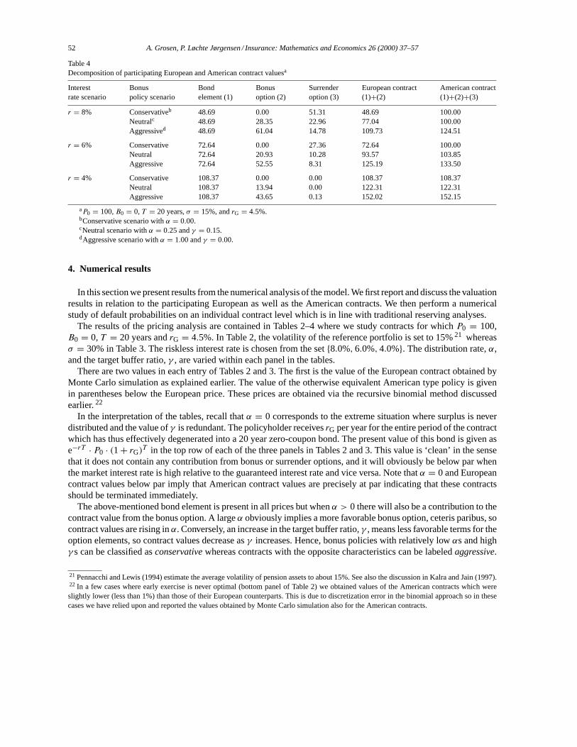
Table 4Decomposition of participating European and American contract valuesa
Interest Bonus Bond Bonus Surrender European contract American contractrate scenario policy scenario element (1) option (2) option (3) (1)+(2) (1)+(2)+(3)
r = 8% Conservativeb 48.69 0.00 51.31 48.69 100.00Neutralc 48.69 28.35 22.96 77.04 100.00Aggressived 48.69 61.04 14.78 109.73 124.51
r = 6% Conservative 72.64 0.00 27.36 72.64 100.00Neutral 72.64 20.93 10.28 93.57 103.85Aggressive 72.64 52.55 8.31 125.19 133.50
r = 4% Conservative 108.37 0.00 0.00 108.37 108.37Neutral 108.37 13.94 0.00 122.31 122.31Aggressive 108.37 43.65 0.13 152.02 152.15
aP0 = 100,B0 = 0, T = 20 years,σ = 15%, andrG = 4.5%.bConservative scenario withα = 0.00.cNeutral scenario withα = 0.25 andγ = 0.15.dAggressive scenario withα = 1.00 andγ = 0.00.
4. Numerical results
In this section we present results from the numerical analysis of the model. We first report and discuss the valuationresults in relation to the participating European as well as the American contracts. We then perform a numericalstudy of default probabilities on an individual contract level which is in line with traditional reserving analyses.
The results of the pricing analysis are contained in Tables 2–4 where we study contracts for whichP0 = 100,B0 = 0, T = 20 years andrG = 4.5%. In Table 2, the volatility of the reference portfolio is set to 15%21 whereasσ = 30% in Table 3. The riskless interest rate is chosen from the set{8.0%, 6.0%, 4.0%}. The distribution rate,α,and the target buffer ratio,γ , are varied within each panel in the tables.
There are two values in each entry of Tables 2 and 3. The first is the value of the European contract obtained byMonte Carlo simulation as explained earlier. The value of the otherwise equivalent American type policy is givenin parentheses below the European price. These prices are obtained via the recursive binomial method discussedearlier.22
In the interpretation of the tables, recall thatα = 0 corresponds to the extreme situation where surplus is neverdistributed and the value ofγ is redundant. The policyholder receivesrG per year for the entire period of the contractwhich has thus effectively degenerated into a 20 year zero-coupon bond. The present value of this bond is given ase−rT · P0 · (1 + rG)T in the top row of each of the three panels in Tables 2 and 3. This value is ‘clean’ in the sensethat it does not contain any contribution from bonus or surrender options, and it will obviously be below par whenthe market interest rate is high relative to the guaranteed interest rate and vice versa. Note thatα = 0 and Europeancontract values below par imply that American contract values are precisely at par indicating that these contractsshould be terminated immediately.
The above-mentioned bond element is present in all prices but whenα > 0 there will also be a contribution to thecontract value from the bonus option. A largeα obviously implies a more favorable bonus option, ceteris paribus, socontract values are rising inα. Conversely, an increase in the target buffer ratio,γ , means less favorable terms for theoption elements, so contract values decrease asγ increases. Hence, bonus policies with relatively lowαs and highγ s can be classified asconservativewhereas contracts with the opposite characteristics can be labeledaggressive.
21 Pennacchi and Lewis (1994) estimate the average volatility of pension assets to about 15%. See also the discussion in Kalra and Jain (1997).22 In a few cases where early exercise is never optimal (bottom panel of Table 2) we obtained values of the American contracts which wereslightly lower (less than 1%) than those of their European counterparts. This is due to discretization error in the binomial approach so in thesecases we have relied upon and reported the values obtained by Monte Carlo simulation also for the American contracts.
A. Grosen, P. Løchte Jørgensen / Insurance: Mathematics and Economics 26 (2000) 37–57 53
In this connection it should be recalled thatγ = 0.00 corresponds to the situation where the life insurance companydoes not aim at building reserves.
Another conclusion is immediate from Tables 2 and 3. It can be seen that constructing par contracts (V0 = 100)is a matter of extreme sensitivity to the distribution policy parametersγ andα. This aspect is further illustrated inTable 4, where the contract values from Tables 2 and 3 have been decomposed into their basic components, i.e. therisk free bond element, the bonus option and the surrender option.
In the tables we see that the American contracts are always more valuable than their European counterparts, thedifference being the value of the surrender option. Also as expected, contract values increase as the bonus policymoves from conservative towards more aggressive. However, note that the value of the surrender option decreaseswith a more aggressive bonus policy. This is quite intuitive since a more aggressive bonus policy is purely to theadvantage of the policyholder. Consequently, his incentive to exercise prematurely may be partly or fully removedin this way.
When the risk free interest rate drops towards and perhaps below the guaranteed interest rate, the contract valueincreases although the value of the option elements decreases. This is explained by the fact that the interest rateguarantee itself moves from being in a senseout of the moneyto beingat or in the money. Being in effect a risklessbond, this contract element of course rises in value when the market interest rate drops. Note at the same time thatthe value of the surrender option decreases as staying in the company becomes more attractive the closer the risklessrate is to the guaranteed interest rate. In other words, the incentive to exercise prematurely will gradually disappearas the market interest rate drops.
The effect of the level of volatility of the underlying portfolio can be seen from comparing Tables 2 and 3. As isusual, option elements become more valuable with increasing uncertainty.
We do not report valuation results for non-zero initial values of the buffer. It is quite clear, however, that if forexampleB0 > 0, the contract values shown in the tables would increase since surplus obtained over the contracts’life would not have to be partly used to build up and maintain the target buffer. Finally, in each panel we indicatetheaverage relative standard errorof the 24 prices obtained by Monte Carlo simulation. The individual standarderrors (not reported) are calculated as the standard error of the Monte Carlo estimate divided by the price estimateitself.
In order to provide a different perspective on the implications of the model, we have extended the simulationanalysis to cover an issue of relevance to the reserving process. Specifically, we have estimated by simulation theprobability of default on the individual contract for various bonus policy parameters. The probabilities reported arerisk neutral, i.e. they areQ-probabilities. These differ from thetrueprobabilities (P -probabilities) to the extent thatthe expected return on assets differ from the risk free rate of interest. We note that obtaining default probabilitiesunder theP -measure would be computationally equivalent but would require a subjective choice of the value of theparameterµ in Eq. (2).
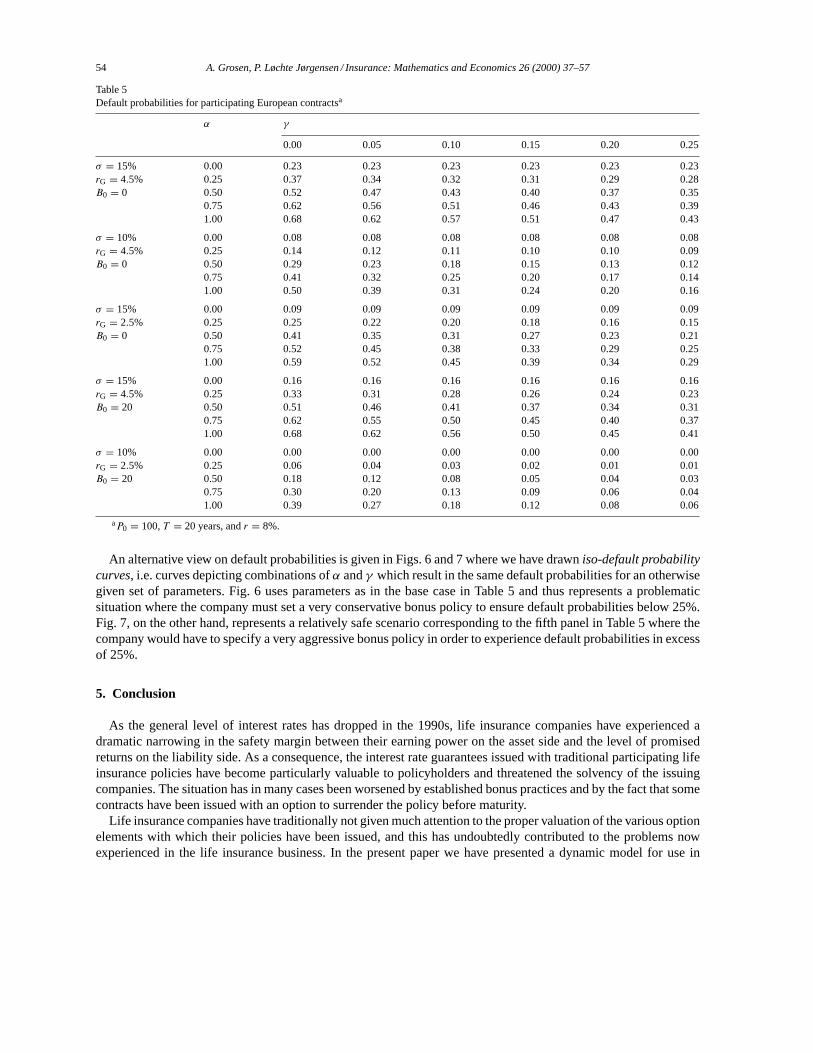
We consider European contracts only and Table 5 contains the estimated default probabilities where default isdefined as the event thatB(T ) < 0. The top panel represents the base case whererG = 4.5%, r = 8%,B0 = 0,andσ = 15%. Different bonus policies are studied by varyingα andγ as in our earlier pricing analysis. Theseparameters are seen to represent a rather risky regime for the insurance company: default probabilities vary between0.23 and 0.68. The following three panels each depicts a situation where we have changed one, and only one,parameter from the base case in a favorable direction as seen from the side of the company. First, the volatility ofassets was lowered to 10%. Second, the guaranteed interest rate was lowered to 2.5%, and third, the initial reserve,B0, was set to 20. In the fifth panel all three changes were applied simultaneously.
The change in volatility from 15% to 10% in the second panel is seen to be quite effectful. For what we considerto be realistic values of the bonus policy parameters, the default probability is more than cut in half. As seenfrom the third panel, the effect on default probabilities of a lowering of the guaranteed interest rate can also bedramatic, whereas for this particular choice of parameters the impact of an initial buffer of substantial size is not thatsignificant (fourth panel). Of course, when the effects are combined as in the fifth panel, the default probabilitiescan be made quite small. This is particularly outspoken when bonus policies are in the conservative to moderatearea.
54 A. Grosen, P. Løchte Jørgensen / Insurance: Mathematics and Economics 26 (2000) 37–57
Table 5Default probabilities for participating European contractsa
α γ
0.00 0.05 0.10 0.15 0.20 0.25
σ = 15% 0.00 0.23 0.23 0.23 0.23 0.23 0.23rG = 4.5% 0.25 0.37 0.34 0.32 0.31 0.29 0.28B0 = 0 0.50 0.52 0.47 0.43 0.40 0.37 0.35
0.75 0.62 0.56 0.51 0.46 0.43 0.391.00 0.68 0.62 0.57 0.51 0.47 0.43
σ = 10% 0.00 0.08 0.08 0.08 0.08 0.08 0.08rG = 4.5% 0.25 0.14 0.12 0.11 0.10 0.10 0.09B0 = 0 0.50 0.29 0.23 0.18 0.15 0.13 0.12
0.75 0.41 0.32 0.25 0.20 0.17 0.141.00 0.50 0.39 0.31 0.24 0.20 0.16
σ = 15% 0.00 0.09 0.09 0.09 0.09 0.09 0.09rG = 2.5% 0.25 0.25 0.22 0.20 0.18 0.16 0.15B0 = 0 0.50 0.41 0.35 0.31 0.27 0.23 0.21
0.75 0.52 0.45 0.38 0.33 0.29 0.251.00 0.59 0.52 0.45 0.39 0.34 0.29
σ = 15% 0.00 0.16 0.16 0.16 0.16 0.16 0.16rG = 4.5% 0.25 0.33 0.31 0.28 0.26 0.24 0.23B0 = 20 0.50 0.51 0.46 0.41 0.37 0.34 0.31
0.75 0.62 0.55 0.50 0.45 0.40 0.371.00 0.68 0.62 0.56 0.50 0.45 0.41
σ = 10% 0.00 0.00 0.00 0.00 0.00 0.00 0.00rG = 2.5% 0.25 0.06 0.04 0.03 0.02 0.01 0.01B0 = 20 0.50 0.18 0.12 0.08 0.05 0.04 0.03
0.75 0.30 0.20 0.13 0.09 0.06 0.041.00 0.39 0.27 0.18 0.12 0.08 0.06
aP0 = 100,T = 20 years, andr = 8%.
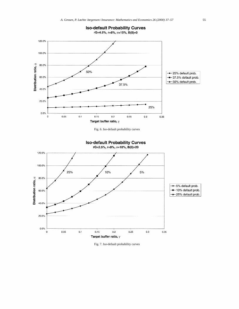
An alternative view on default probabilities is given in Figs. 6 and 7 where we have drawniso-default probabilitycurves, i.e. curves depicting combinations ofα andγ which result in the same default probabilities for an otherwisegiven set of parameters. Fig. 6 uses parameters as in the base case in Table 5 and thus represents a problematicsituation where the company must set a very conservative bonus policy to ensure default probabilities below 25%.Fig. 7, on the other hand, represents a relatively safe scenario corresponding to the fifth panel in Table 5 where thecompany would have to specify a very aggressive bonus policy in order to experience default probabilities in excessof 25%.
5. Conclusion
As the general level of interest rates has dropped in the 1990s, life insurance companies have experienced adramatic narrowing in the safety margin between their earning power on the asset side and the level of promisedreturns on the liability side. As a consequence, the interest rate guarantees issued with traditional participating lifeinsurance policies have become particularly valuable to policyholders and threatened the solvency of the issuingcompanies. The situation has in many cases been worsened by established bonus practices and by the fact that somecontracts have been issued with an option to surrender the policy before maturity.
Life insurance companies have traditionally not given much attention to the proper valuation of the various optionelements with which their policies have been issued, and this has undoubtedly contributed to the problems nowexperienced in the life insurance business. In the present paper we have presented a dynamic model for use in
A. Grosen, P. Løchte Jørgensen / Insurance: Mathematics and Economics 26 (2000) 37–57 55
Fig. 6. Iso-default probability curves
Fig. 7. Iso-default probability curves
56 A. Grosen, P. Løchte Jørgensen / Insurance: Mathematics and Economics 26 (2000) 37–57
valuing the common family of life insurance products known as participating contracts. The model is based on thewell-developed theory of contingent claims valuation. We have shown that the typical contract can be decomposedinto three basic elements: a risk free bond, an option to receive bonus, and a surrender option.
The properties of the model were explored numerically. The analysis showed that contract values are highlydependent on the assumed bonus policy and on the spread between the market interest rate and the guaranteed rateof interest built into the contract. In another application of the model, we estimated by simulation the relation betweenbonus policies and the probability of default at the individual contract level. This analysis showed default probabilitiesof substantial size for realistic parameter choices indicating that the management of the life insurance companyshould take solvency problems very seriously. In this respect, initiatives on both the asset and the liability sides couldbe considered. An obvious first choice could be to reduce asset volatility by changing the asset composition towardsless risky assets. But another potential problem enters here. The return offered by less risky assets (bonds) mightbe so low that such a move would only make it certain that interest guarantees could not be honored in the future.A classical asset substitution problem where the company management is forced into taking risks might thus exist.Alternatively, to reduce the probability of default, the company could consider more conservative bonus policiesto the extent that this is permitted by law and the contractual terms. In fact, the possibility for the management tochange the bonus policy parameters in a sense constitutes acounter optionwhich we have not explicitly taken intoaccount in this paper. This is an interesting subject for future research as would be the analysis of how the asset mixcould possibly be optimally described as a function of the liability situation of the life insurance company.
Some other natural paths for further research emerge. In the present article, a model was constructed in orderto describe actual insurance company behavior with particular respect to applied accounting principles and bonuspolicies. Future research should try to establish the ideal way in the sense that systematic market value accountingshould constitute the basis of the balance sheet as well as the bonus policy. Furthermore, realism could obviously beadded to the model by considering periodic premiums and taking into account mortality, lapses and various expensecharges. Lastly, an interesting issue would be to incorporate the possibility of default of the life insurance companyand to analyze how this would affect contract values and possibly also the optimal surrender strategy.
Acknowledgements
We are grateful for the comments of an anonymous referee, Phelim P. Boyle, Paul Brüniche-Olsen, KristianR. Miltersen, Claus Parum, Jens Perch-Nielsen, Svein-Arne Persson, Henrik Ramlau-Hansen, Carsten Tanggaard,workshop participants at the Danish Society for Actuaries, participants at the 1998 Danske Bank Symposium onSecurities with Embedded Options, the 1999 Conference on Financial Markets in the Nordic Countries, the 26thseminar of the European Group of Risk and Insurance Economists, the 9th International AFIR Colloquium, the20th Annual Meeting of the European Finance Association, and at the Third International Congress on Insurance:Mathematics and Economics. The usual disclaimer applies. Financial support from the Danish Natural and SocialScience Research Councils is gratefully acknowledged.
References
Babbel, D.F., Merrill, C., 1999. Economic valuation models for insurers. North American Actuarial Journal. Forthcoming.Baccinello, A.R., Ortu, F., 1993a. Pricing equity-linked life insurance with endogenous minimum guarantees. Insurance: Mathematics and
Economics 12 (3), 245–258.Baccinello, A.R., Ortu, F., 1993b. Pricing equity-linked life insurance with endogenous minimum guarantees: a corrigendum. Insurance:
Mathematics and Economics 13, 303–304.Black, F., Scholes, M., 1973. The pricing of options and corporate liabilities. Journal of Political Economy 81 (3), 637–654.Black, K., Skipper, H.D., 1994. Life Insurance, 12th ed. Prentice Hall, Englewood Cliffs, NJ.Boyle, P.P., 1977. Options: a Monte Carlo approach. Journal of Financial Economics 4, 323–338.Boyle, P.P., Broadie, M., Glasserman, P., 1997. Monte Carlo methods for security pricing. Journal of Economic Dynamics and Control 21,
1267–1321.

A. Grosen, P. Løchte Jørgensen / Insurance: Mathematics and Economics 26 (2000) 37–57 57
Boyle, P.P., Hardy, M.R., 1997. Reserving for maturity guarantees: two approaches. Insurance: Mathematics and Economics 21, 113–127.Boyle, P.P., Schwartz, E.S., 1977. Equilibrium prices of guarantees under equity-linked contracts. Journal of Risk and Insurance 44, 639–660.Brennan, M.J., 1993. Aspects of insurance, intermediation and finance. The Geneva Papers on Risk and Insurance Theory 18 (1), 7–30.Brennan, M.J., Schwartz, E.S., 1976. The pricing of equity-linked life insurance policies with an asset value guarantee. Journal of Financial
Economics 3, 195–213.Brennan, M.J., Schwartz, E.S., 1979. Alternative investment strategies for the issuers of equity-linked life insurance policies with an asset value
guarantee. Journal of Business 52 (1), 63–93.Briys, E., de Varenne, F., 1997. On the risk of life insurance liabilities: debunking some common pitfalls. Journal of Risk and Insurance 64 (4),
673–694.Broadie, M., Glasserman, P., 1997. Pricing American-style securities using simulation. Journal of Economic Dynamics and Control 21, 1323–
1352.Cox, J.C., Ross, S.A., Rubinstein, M., Ross and Rubinstein, 1. Option pricing: a simplified approach. Journal of Financial Economics 7, 229–263.Embrechts, P., 1996. Actuarial versus financial pricing of insurance. Working paper. Wharton Financial Institutions Center, WP 96-17.Gentle, J.E., 1998. Random Number Generation and Monte Carlo Methods. Springer, New York.Grosen, A., Jørgensen, P.L., 1997. Valuation of early exercisable interest rate guarantees. Journal of Risk and Insurance 64 (3), 481–503.Harrison, M.J., Kreps, D.M., 1979. Martingales and arbitrage in multiperiod securities markets. Journal of Economic Theory 20, 381–408.Hull, J.C., 1997. Options, Futures, and other Derivatives, 3rd ed. Prentice-Hall, Englewood Cliffs, NJ.Kalra, R., Jain, G., 1997. A continuous-time model to determine the intervention policy for PBGC. Journal of Banking and Finance 21, 1159–1177.Karatzas, I., 1988. On the pricing of the American option. Applied Mathematics and Optimization 17, 37–60.Maturity Guarantees Working Party, 1980. Report. Journal of the Institute of Actuaries 107, 103–209.Miltersen, K.R., Persson, S.A., 1998. Guaranteed investment contracts: distributed and undistributed excess return. Working paper. Odense
University, Odense.Nielsen, J.A., Sandmann, K., 1995. Equity-linked life insurance: a model with stochastic interest rates. Insurance: Mathematics and Economics
16, 225–253.Nielsen, J.P., Thaning, H.L., 1996. Matching of assets and liabilities in Danish pension companies. Working paper. PFA Pension and Copenhagen
Business School.Parum, C., 1999. Historical returns on stocks and bonds in Denmark. Finans/Invest (III), 4–13 (in Danish).Pennacchi, G., Lewis, C., 1994. The value of pension benefit guarantee corporation insurance. Journal of Money, Credit and Banking 26,
735–753.Press, W.H., Flannery, B.P., Teukolsky, S.A., Vetterling, W.T., 1989. Numerical Recipes in Pascal. Cambridge University Press, Cambridge.Quandt, R., 1983. Computational problems and methods. In: Griliches, Z., Intriligator, M. Eds., Handbook of Econometrics, cha. 12, vol. 1.
North-Holland, Amsterdam.Tilley, J., 1993. Valuing American options in a path simulation model. Transactions of the Society of Actuaries 45, 83–104.Vanderhoof, I.T., Altman, E.I. (Eds.), 1998. The Fair Value of Insurance Liabilities, Kluwer Academic Publishers, Dordrecht. The New York
University Salomon Center Series on Financial Markets and Institutions.