Fair Valuation of Life Insurance Liabilities: The Impact of Interest Rate Guarantees, Surrender Options, and Bonus Policies*

Anders Grosen

Department of Finance

Aarhus School of Business

DK-8210 Aarhus V DENMARK

Tel. + 45 89 48 64 21

Tel. + 45 86 15 19 43 e-mail: gro@hha.dk

Peter Lachte Jwgensent

Department of Management

University of Aarhus, Bldg. 350 DK-8000 Aarhus C

DENMARK

Tel. + 45 89 42 15 44 Fax. + 45 86 13 51 32

e-mail: ecolochte@econ.au.dk

First version: September, 19!# Current version: March 31,1999

*We are grateful for the comments of Phelim P. Boyle, Paul BNniche-Olsen, Kristian R. Miltersen, iens Perch- Nielsen, Svein-Ame Petsson, Henrik Ramlau-Hansen, Carsten Tauggaard, workshop participants at the Danish Society for Actuaries, and participants at the 1998 Danske Bauk Symposium on Securities with Embedded Options and at the 1999 Conference on Financial Ma&e& in the Nordic Cuuntries. The usual disclaimer applies. Financial suppurt from the Danish Natural and Social Science Research Councils is gratefidly acknowledged. Docnnmt typeset in l5T&

+Corre.sponding author.

-221-

Abstract

The paper analyzes one of the most common life insurance products - the so-called

participariflg (or with pro@) policy. This type of contract stands in contrast to Unit-

Linked (UL) products in that interest is credited to the policy periodically according to

some mechanism which smoothes past returns on the life insurance company’s (LIC)

assets. As is the case for UL products, the participating policies are typically equipped

with an interest rate guarantee and possibly also an option to surmnder (sell-back) the

policy to the LIC before maturity.

The paper shows that the typical participating policy can be decomposed into a risk free

bond element, a bonus option, and a surrender option. A dynamic model is constructed

in which these elements can be valued separately using contingent claims analysis. The

impact of various bonus policies and various levels of the guaranteed interest rate is

analyzed numerically. We find that values of participating policies are highly sensitive

to the bonus policy, that surrender options can be quite valuable, and that LIC solvency

can be quickly jeopardized if earning opportunities deteriorate in a situation where bonus

reserves are low and promised returns are high.

JEL Classification Codes: G13, G22, and G23.

Subject/Insurance Branche Codes: IMlO and IEOl.

Keywords: Participating Life Insurance Policies, embedded options, contingent claims valu-

ation, bonus Policy, surrender.

-222-

1 Introduction

Embedded options pervade the wide range of products offered by pension funds and life

insurance companies. Interest rate guarantees, bonus distribution schemes, and surrender

possibilities are common examples of implicit option elements in standard type policies issued

in the United States, Europe, as well as in Japan. Such issued guarantees and written options

are liabilities to the issuer. They represent a value and constitute a potential hazard to company

solvency and these contract elements should therefore ideally be properly valued and reported

separately on the liability side of the balance sheet. But historically this has not been done,

to which there are a number of possible explanations. Firstly, it is likely that some companies

have failed to realize that their policies in fact comprised multiple components, some of which

were shorted options. Secondly, it seems fair to speculate that other companies have simply

not cared. The options embedded in their policies may have appeared so far out of the

money, in particular at the time of issuance, that company actuaries have considered the costs

associated with proper assessment of their otherwise neglegible value to far outweigh any

benefits. Thirdly, the lack of analytical tools for the valuation of these particular obligations

may have played a part. Whatever the reason, we now know that the negligence turned out

to be catastrophic for some companies, and as a result shareholders and policyowners have

suffered. Jn the United States, a large number of companies have been unable to meet their

obligations and have simply defaulted (see e.g. Briys and de Varenne (1997) and the references

cited therein for details), whereas in e.g. the United Kingdom and Denmark, companies have

started cutting their bonuses in order to ensure survival.

The main trigger for these unfortunate events is found on the other side of the balance

sheet where life insurance companies have experienced significantly lower rates of return on

their assets than in the 1970s and 1980s. The lower asset returns in combination with the

reluctance of insurance and pension companies to adjust their interest rate guarantees on new

policies according to prevailing market conditions have resulted in a dramatic narrowing of

the safety margin between the companies’ earning power and the level of the promised returns.

Stated differently, the issued interest rate guarantees have moved from being far out of the

-223-

money to being very much in he money, and many companies have experienced solvency

problems as a result. The reality of this threat has most recently been illustrated in Japan

where Nissan Mutual life insurance group collapsed as the company failed to meet interest

rate guarantees of 4.7% p.a.t Nissan Mutual’s uncovered liabilities were estimated to amount

to $ 2.56 billion, so in this case policyholders’ options indeed expired in the money without

the company being able to fulfil its obligations.

Partly as a result of Nissan Mutual Life’s collapse, Japanese life insurance companies

have been ordered to reduce the interest rate guarantee from 4.5% to 2.5% p.a. In Europe,

the EU authorities have also responded to the threat of insolvency from return guarantees.

Specifically, Article 18 of the Third EU Life Insurance Directive, which was effective as of

November 10, 1992, requires that interest rate guarantees do not exceed 60% of the rate of

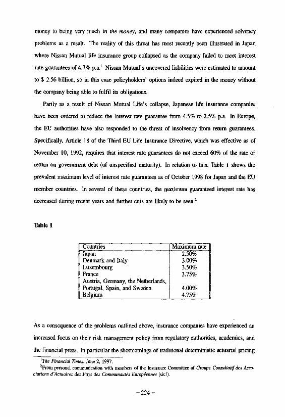
return on government debt (of unspecified maturity). In relation to this, Table 1 shows the

prevalent maximum level of interest rate guarantees as of October 1998 for Japan and the EU

member countries. In several of these countries, the maximum guaranteed interest rate has

decreased during recent years and further cuts are likely to be seen.2

Table 1

Countries Maximum rate Japan 2.50% Denmark and Italy 3.00% Luxembourg 3.50% France 3.75% Austria, Germany, the Netherlands, Portugal, Spain, and Sweden 4.00% Beleium 4.75%

As a consequence of the problems outlined above, insurance companies have experienced an

increased focus on their risk management policy from regulatory authorities, academics, and

the financial press. In particular the shortcomings of traditional deterministic actuarial pricing

‘The Financial Zimes, June 2, 1997. “From personal canmunication with members of the Insurance Committee of Group Cot~rul~a?~ des ASSO-

ciations d’Actuaires des Pays des CommunourGs Eumpt?eennes (sic!).

-224-

principles when it comes to the valuation of option elements are surfacing. Recent years have

also revealed an increasing interest in applying financial pricing techniques to the fair valuation

of insurance liabilities, see for example Babbel and Merrill (1999) Boyle and Hardy (1997).

and Vanderhoof and Altman (1998).3

In the literature dealing with the valuation of and to some extent also the reserving for

insurance liabilities, several types of contracts and associated guarantees and option elements

are recognized. Some of the contracts considered contain option elements of European type,

meaning that the option(s) can be exercised only at maturity. This contrasts American type

contracts where the embedded option(s) can be exercised at any time during the life of the

contract. Another important distinction must be made between unit-linked contracts4 and con-

tracts where interest is credited according to some smoothing surplus distribution mechanism.

The latter type is generally known as participating contracts and the interest rate crediting

mechanism applied is often referred to as a portfolio average method or an average interest

principle. Finally, in relation to guarantees it is important to distinguish between maturity

guarantees and interest rate guarantees (rate of return guarantees). A maturity guarantee is a

promise to repay at least some absolute amount at maturity (75% of the initial deposit, say)

whereas an interest rate guarantee promises to credit the account balance with some minimum

return every pet+~I.~

While participating policies are by far the most important in terms of market size, the larger

part of the previous literature in this area has been analyzing unit-linked contracts with interest

rate or maturity guarantees of the European type (Boyle and Schwartz (1977) Brennan and

Schwartz (1976), Brennan and Schwartz (1979), Baccinello and Ortu (1993a), Nielsen and

‘The concern about traditional deterministic actuarial pricing principles and in particular the principle of equivalence is not entirely new. In the United Kingdom, the valuation of mahm’ry gr4aranree.s (as opposed to the inreresr rare guoranrees studied in the present paper) was a concern twenty years ago when tire Institute of Actuaries commissioned the Report of the Maturity Guarantees Working Party (1980), in which the valuation of maturity guarantees in life insurance was studied (see also the discussion in Boyle and Hardy (1997)). It was recognized that a guarantee has a cost and that explicit payment for these guarantees is necessary. For an interesting view and a discussion of actuarial vs. financial pricing, the reader is referred to Embrechts (1996).

4A policy is unit-linked (equity-linked) if the interest rate credited to the customer’s account is linked directly and without lags to the return on some reference (equity) portfolio the unit.

‘Maturity guarantees and interest rate guarantees are obviously equivalent for single period contracts. How- ever, in a multiple period setting where the interest rate guarantee is on the current account balance and interest is credited according to the principle that “what has once been given, can never be taken away” there is a significant difference between these two types of guarantees.

-225-

Sandmann (1995) and Boyle and Hardy (1997)). Some notable exceptions to this are the works

by Brennan (1993), Briys and de Varenne (1997) Miltersen and Persson (1998), and Grosen

and Jorgensen (1997). Inspired by classic UK with profits policies, Brennan (1993) discusses

the efficiency costs of the reversionary bonus mechanism applied to these contracts. In their

analysis of the valuation and duration of life insurance liabilities, Briys and de Varenne (1997)

explicitly introduce a patiicipation level in addition to the guaranteed interest rate attached to

policies. However, the model is essentially a single period model where distinctions between

interest rate and maturity guarantees and between guarantees of European and American type

become less interesting. Miltersen and Persson (1998) present another interesting model in

which contracts with an interest rate guarantee and a claim on excess returns can be valued.

To model a kind of participation, the authors introduce a bonus account to which a part of

the return on assets is distributed in ‘good’ years and from which funds can be withdrawn

and used to fulfil the interest rate guarantee in poor years. The drawbacks of this model are

that no averaging or smoothing is built into the distribution mechanism, and that the bonus

account, if positive at maturity, is paid out in full to policyholders. This is a somewhat

unrealistic assumption. Also the American type surrender option is not considered in this

model. In Grosen and Jorgensen (1997), arbitrage-free prices of unit-linked contracts with an

early exercisable (American) interest rate guarantee are obtained by the application of American

option pricing theory. They also point out that the value of the option to exercise prematurely

is precisely the value of the the surrender option implicit in many life insurance contracts.

The numerical work in Grosen and Jorgensen (1997) demonstrates that this particular option

element may have significant value and hence that it must not be overlooked when the risk

characteristics of liabilities are analyzed and reserving decisions are made. However, the

contracts considered in their paper are unit-linked and bonus mechanisms are not considered.

The present paper attempts to fill a gap in the existing literature by extending the analysis

in Grosen and Jorgensen (1997) from unit-linked contracts to traditional participating policies,

i.e. to contracts in which some surplus distribution mechanism is employed each period to

credit interest at or above the guaranteed rate. The objective is thus to specify a model which

encompasses the common characteristics of life insurance contracts discussed above and which

-226-

can be used for valuation and risk analysis in relation to these particular liabilities. Our work

towards this goal will meet a chain of distinct challenges: First, asset returns must be credibly

modeled. In this respect we take a completely non-controversial approach and adopt the widely

used framework of Black and Scholes (1973). Second, and more importantly, a realistic model

for bonus distribution must be specified in a way that integrates the interest rate guarantee. This

is where our main contributions lie. The third challenge is primarily of technical nature and

concerns the arbitrage-free valuation of the highly path-dependent contract pay-offs resulting

from applying the particular bonus distribution mechanism suggested to customer accounts. We

will carefully take interest rate guarantees as well as possible surrender options into account

and during the course of the analysis we also briefly touch upon the associated problem

of reserving for the liabilities. Finally, we provide a variety of illustrative examples. The

numerical section of the paper also contains some insights into the effective implementation

of numerical algorithms for solving the model.

The paper is organized as follows. Section 2 describes the products which will be analyzed

and presents the basic modelling framework. In particular, the bonus policy and the dynamics

of assets and liabilities are discussed. In section 3 we present the methodology applied for

contract valuation, we demonstrate how contract values can be conveniently decomposed into

their basic elements, and computational aspects are addressed. Numerical results are presented

in section 4, and section 5 concludes the paper.

-227-

2 The Model

In this section we provide a more detailed description of the life insurance contracts and

pension plan products which we will analyze. Furthermore, we introduce the basic model to

be used in the analysis and valuation of these contracts - especially the valuation of various

embedded option elements.

The basic framework is as follows. Agents are assumed to operate in a continuous time

frictionless economy with a perfect financial market, so that tax effects, transaction costs,

divisibility, liquidity, and short-sales constraints and other imperfections can be ignored. As

regards the specific contracts, we also ignore the effects of expense charges, lapses and mor-

tality.6

At time zero (the beginning of year one) the policyholder makes a single-sum deposit,

VO, with the insurance compar~y.~ He thereby acquires a policy or a contract of nominal

value PO which we will treat as a financial asset, or more precisely, as a contingent claim.

in general, we will treat Pa as being exogenous whereas the fair value of the contract, I&, is

to be determined. VO may be smaller or larger than PO depending on the contractual terms -

particularly the various option elements. The policy matures after T years when the account

is settled by a single payment from the insurance company to the policyholder. However, in

some cases to be further discussed below, we will allow the policy to be terminated at the

policyholder’s discretion prior to time T.

At the inception of the contract, the insurance company invests the tmsted funds in the

financial market and commits to crediting interest on the policy’s account balance according

to some pay-out scheme linked to each year’s market return until the contract expires. We will

discuss the terms for the market investment and the exact nature of this interest rate crediting

’ Since we ignore the insurance aspects mentioned and focus entirely on financial risks, the reader may also simply think of the products analyzed as a specific form of guaranteed invemnent contracts (GICs). In general,

GlCs in their various forms have been a significant investment vehicle for pension plans over the last 20 years. In

the early 199Os, confideace in GlCs was seriously shaken by the financial troubles of some insurance companies that were affected by defaults of junk bonds they purchased in the 1980s and poor m&gage loan results. GlCs do not generally enjoy the status of ‘insurance’, and therefore they are not entitled to state guarantee fund coverage in the event of defaults, (Black and Skipper (1994). p. 814-815.)

‘The extension to periodic premiums is straightforward, but omitted owing to space considerations.

-228-

mechanism in more detail shortly. For now we merely note that the interest rate credited to

the policy in year t, i.e. from time t - 1 to time t, is denoted rp(t) and is guaranteed never

to fall below ro, the constant, positive, and contractually specified guaranteed annual policy

interest rate. Both rates are compounded annually.

The positive difference between the policy interest rate credited in year t and the guaranteed

rate is denoted the bonus interest rate, Tg(t), and we obviously have

TB(t) = T)(t) - ‘?.c: 2 0, v t. (1)

The final interest rate to be introduced is the economy’s (continuously compounded) riskless

rate of interest. We denote it by T and assume that it is a constant.*

It is obvious that the interest rate crediting mechanism, i.e. the policy for the determina-

tion of each year’s rp(.) (or equivalently rg(‘)), is of vital importance for the value of the

policyholder’s claim. We now turn to the discussion and our modelling of this key issue.

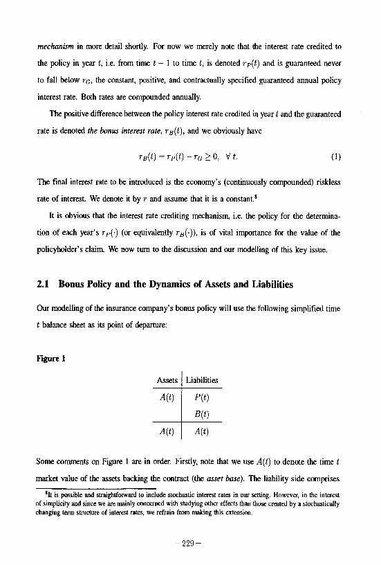
2.1 Bonus Policy and the Dynamics of Assets and Liabilities

Our modelling of the insurance company’s bonus policy will use the. following simplified time

t balance sheet as its point of departure:

Some comments on Figure 1 are in order. Firstly, note that we use A(t) to denote the time t

market value of the assets backing the contract (the asset base). The liability side comprises

*It is possible and straightforward to include stochastic interest rates in our setting. However, in the interest of simplicity and since we are mainly concerned with studying other effects than those created by a stochastically changing term structure of interest rates, we refrain from making this extension.

-229-

two entries: P(t) is the policyholder’s account balance or, briefly, the policy reserve, whereas

B(t) is the bonus reserve. Actuaries also often denote B(t) simply as the buffer. Although

added up, these two entities equal the market value of the assets, individually they are not

market values. The policy reserve, P(t), is rather a book value, whereas B(t) is a hybrid

being residually determined as a difference between a market value and a book value. This

construction is applied out of a wish to model actual insurance company behavior rather than

in an attempt to describe fhe ideal way. Furthermore, we emphasize that since we have chosen

to focus on individual policies (or, alternatively, a cohort of identical policies), Figure 1 is @

the company balance sheet but rather a snap-shot of the asset and liability situation at a certain

point in time and in relation to some specified policy (cohort of policies). Finally, we note

that ‘equity’ is not missing from the liability side of Figure 1. Since in many cases the owner

and the policyholders of the insurance company are the same, it is not essential to distinguish

between bonus reserves, i.e. the amount allocated for future distribution, and equity. Hence,

we have not included ‘equity’ as a separate entry on the liability side of the balance sheet.

2.1.1 The Asset Side of the Balance Sheet

The insurance company is assumed to keep the asset base invested in a well-diversified and

well-specified reference portfolio at all times. Recall that we use A(t) to denote the time

t market value of this investment. No assumptions are made regarding the composition of

this portfolio with respect to equities, bonds, real estate, or regarding the dynamics of its

individual elements. We simply work on an aggregate level and assume that the total market

value evolves according to a geometric Brownian motion9

dA(t) = pA(t) dt + aA &V(t), A(0) = A,,. (2)

‘The assumption that assets evolve according to the GBM is not motivated by a wish to obtain Closed/arm or analytic solutions to the problems studied. Indeed, doe to the complexity of the contract pay-offs, we obtain no such solutions and we resort instead to extensive use of numerical methods. The numerical analysis could just as easily be carried out using another model for the evolution in asset values. Actoariea, for example, may prefer to apply the Wilkie model to describe the evolution of asset values (see e.g. Boyle and Hardy (1997)). Another interesting possibility is to let assets evolve according to a jump-diffusion model.

-230-

Here p, 0, and A0 are constants and IV(.) is a standard Brownian motion defined on the

filtered probability space (n, F, (3;), P) on the finite interval [0, T].”

For the remaining part of the paper we shall work under the familiar equivalent risk neutral

probability measure, Q, (see e.g. Harrison and Kreps (1979)) under which discounted prices

are Q-martingales and where we have

dA(t) = rA(t) dt + aA dWQ(t), A(o) = A,, (3)

and where Wu(.) is a standard Brownian motion under Q. The stochastic differential equation

in (3) has a well-known solution given by

A(t) = An. e(r-$‘2)~+~~Q(~) (4)

In particular, we will need to work with annual (log) returns which are easily established as

conditionally normal:

2.1.2 The Liability Side of the Balance Sheet

We now direct our attention towards describing the dynamics of the liability side of the balance

sheet. Referring to Figure 1, we have previously introduced the two entries P(t) and B(t)

as the policy reserve and the bonus reserve, or alternatively, as the policyholder’s account

balance and the buffer. Regardless of terminology, it is important not to confuse P(t) with

the concurrent fair value of the policy.

The distribution of funds to the two liability entries over time is determined by the bonus

policy, i.e. by the sequence rp(t) for t E r E { 1,2,. , T}. In particular, note that from the

‘@The assumption that p is constant is made for simplicity and is a bit stronger than necessary. As pointed oat by Black and Scholes (1973), standard arbitrage valuation carries through witbwt changes if we allow p to depend on time and/or the current state.

- 231 --

earlier definition of the policy interest rate we must have

P(t) = (1 + T-p(t)) . P@ - l), t E T, (6)

from which we deduce

P(t) = P&l + q-(i)), t E I-. (7) i=l

These are obviously two rather empty expressions until we know more about the determinants

of the process followed by TP(.), i.e. the interest rate crediting mechanism. Not until more

has been said about this issue can we start to study the dynamics of the liability side of the

balance sheet (in particular the policyholder’s account) and the valuation of the policyholder’s

contract.

The question of how rP(.) is determined in practice is highly subtle involving intangible

political, legal, and strategic considerations within the insurance company. There is therefore

little hope that we can ever construct simple models which can precisely capture all elements

of this process. In particular, the theoretical possibility for the management of the insurance

company to change the surplus distribution policy over time -perhaps within specific limits set

by law - will be problematic for the task of valuing the policyholder’s claim. Put differently,

this means that whenever we apply and analyze a certain interest rate crediting mechanism in

our models, we should keep in mind that we are not necessarily dealing with strictly (legally)

binding agreements between the parties.

Having realized these problems - of which we are unaware of parallels in the standard

financial (exotic) options literature - we will proceed with an attempt to specify an interest

rate crediting mechanism which is as accurate and realistic an approximation to the true bonus

policy as possible. We shall specify the interest rate crediting mechanism in the form of some

mathematically well-defined function in order to be able to apply the powerful apparatus of

financial mathematics and, in particular, arbitrage pricing.

While problems do exist as outlined above, there are fortunately also some well-established

principles that can be used as inspiration. Firstly, it is clear that realized returns on the assets

in a given year must influence the policy interest rate in the ensuing year(s). Secondly,

-232-

since one of the main arguments in the marketing of these life insurance policies is that they

provide a low-risk, stable, and yet competitive return compared with other marketed assets,

our modelling of the interest rate crediting mechanism should also accomplish this. The

surplus distribution rule should in other words resemble what is known in the industry as the

average interest principle. ” Thirdly, in order to provide these stable returns to policyholders12

and to partially protect themselves against insolvency, the life insurance companies aim at

building and maintaining a certain level of reserves (the buffer). This could and should also

be accounted for in constructing the distribution rule.

In sum, an attempt to model actual interest rate crediting behavior of life insurance compa-

nies should involve the specification of a functional relationship from the asset base, A(.), and

the bonus reserve, B(.), to the policy interest rate, rp(t). In this way, the annual interest bonus

can be based on the actual investment perfotmance as well as on the current financial position

(the degree of solvency) of the life insurance company. Furthermore, the functional relation-

ship should be constructed in such a way that policy interest rates are in effect low-volatility,

smoothed market returns.

We thus propose to proceed in the following way. It is fist assumed that the insurance

company’s management has specified a constant target for the ratio of bonus reserves to policy

reserves, i.e. the ratio #. We call this the target h&r ratio and denote it by y. A realistic

value would be in the order of l&15%. Suppose further that it is the insurance company’s

objective to distribute to policyholders’ accounts a positive fraction, Q, of any excessive bonus

reserve in each period. The company must, however, always credit at least the guaranteed

rate, TG, which it will do if the bonus reserve is insufficient or even negative. Clearly for

appropriate values of cr this mechanism will ensure a stable smoothing of the surplus. The

“The average interest principle is discussed in e.g. Nielsen and Thaning (1996). These authors write I‘ the average interest principle used by most of the pension business, partly to assure the customer a pcsitive yield each year and partly to minimize the companies’ risk due to the interest guarantee given means that the yield given to the insured is very different from the companies’ yield on investments each year. The difference is regulated by the swAed dividend equalisation provisions.”

‘*insurance companies sometimes label their bonus reserves bonus smoothing reserves’ indicating their role in sustaining the average interest principle.

-233-

coefficient N is referred to as the distribution ratio. I3 A realistic value of a is in the area of

20-30%. Before we proceed, let us briefly recapitulate the most frequently applied notation:

PO T

dt) TG

T/r(t)

Ai w w

Y (Y u

policy account balance at time 0 maturity date of the contract policy interest rate in year t guaranteed interest rate bonus interest rate in year t riskless interest rate market value of insurance company’s assets at time t policy reserve at time t bonus reserve at time t target buffer ratio distribution ratio asset volatility

(8)

The discussion above can now be formalized by setting up the following analytical scheme

for the interest rate credited to policyholders’ accounts in year t,

-- 7

)> .

This implies a bonus interest rate as stated below,

(9)

(10)

Note fist that as in real life contracts, the interest rate credited between time t - 1 and time t

is determined at time t - 1, i.e. there is a degree of predictability in the interest rate crediting

mechanism.‘4 observe also that when TG < a (M-7) (reservesare‘high’)wecanwrite

P(t) = P(t - 1) 1 +o(H -7))

= P(t - 1) + a(B(t - 1) - TP(t - 1))

= P(t - 1) + a(B(t - 1) - B*(t - 1)),

“Briys and de Varenne (1997) work with a similar parameter called the participation coeficienf. 141n Denmark, for example, all major insurance companies announce their policy interest rate for the coming

year in mid-december the year before.

-234-

where B*(t - 1) z yP(t ~ 1) denotes the optimal reserve at time t - 1. Hence, when reserves

are satisfactorily large, a fixed fraction of the excessive reserve is distributed to policyholders.r5

Returning to the general evolution of the policyholder’s account, we have the relation

P(t) = P(t- 1) (l+max{T,,@+)})

zz P(t-1) l+rc+max 0,cy 1 (

4 - 1) - W - 1) _ y P(t ~ 1) > }) . (12)

~ Tc

This difference equation clarifies a couple of points. Firstly, it is seen that the interest rate

guarantee implies a floor under the final payout from the contract. The floor is given as

P,,&+,(T) = (1 +r~)“‘. P(0) and it becomes effective in case bonus is never distributed to the

policy. But note also that as soon as bonus has been distributed once, the floor is lifted since

the guaranteed interest rate applies to the initial balance, accumulated interest, and bonus. We

can therefore conclude that there is a risk free bond element to the contract implied by the

interest rate guarantee. Secondly, expression (12) clarifies that the bonus mechanism is indeed

an option element of the contract.

At this point it would have been convenient if from (12) we could establish the probabilistic

distribution followed by P(T). However, recursive substitution of the P(.)s quickly gets

complicated and P(T) is obviously highly dependent on the path followed by A(.). The path

dependence of the policyholder’s account balance eliminates any hope of finding analytical

expressions for the contract values. However, them is a wide range of numerical methods

at our disposal to deal with this kind of problem. We will start looking at these in the next

section. The present section is rounded off with some plots of simulation runs of the model

to give the reader a feel for how things work.

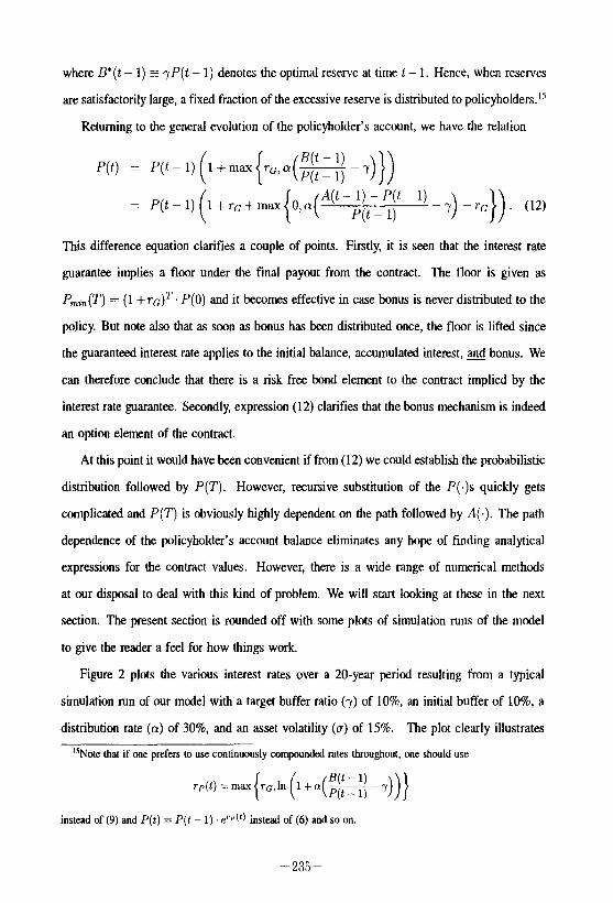
Figure 2 plots the various interest rates over a 20-year period resulting from a typical

simulation run of our model with a target buffer ratio (y) of lo%, an initial buffer of lo%, a

distribution rate (o) of 30%, and an asset volatility ((T) of 15%. The plot clearly illustrates

ISNote that if one prefers to use continuously compounded rates throughout, one should use

instead of (9) and P(t) = P(t - 1) c?‘J’(‘) instead of (6) and so on

-235-

Simulated Market Return and Policy Interest Rate rG.4.5%, r=8%,0=15%, w30%,~10%, B(O)=lO, P(O)=100

0.3 -___---.- _..___...-. - --..--.--.. --.---- J Ttmc h yews

Figure 2: Simulated market return and policy interest rate

the smoothing that takes place in the policy interest rate. These rates vary much less than the

market return on assets. Moreover, they are bounded below by the guaranteed rate of interest

of 4.5% which comes into effect in certain years. Put differently, in some years there is no

bonus whereas in other years the policy interest rate is quite generous compared with the risk

free rate which is set at 8% in this example.

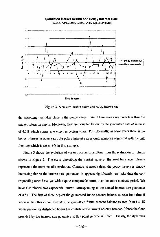
Figure 3 shows the evolution of various accounts resulting from the realisation of returns

shown in Figure 2. The curve describing the market value of the asset base again clearly

represents the more volatile evolution. Contrary to asset values, the policy reserve is strictly

increasing due to the interest rate guarantee. It appears significantly less risky than the cor-

responding asset base, yet with a quite comparable return over the entire contract period. We

have also plotted two exponential curves corresponding to the annual interest rate guarantee

of 4.5%. The first of these depicts the guaranteed future account balance as seen from time 0

whereas the other curve illustrates the guaranbxd future account balance as seen from t = 15

where previously distributed bonus has contributed to current account balance. Hence the floor

provided by the interest rate guarantee at this point in time is ‘lifted’. Finally, the dynamics

-236-

Simulated Evolution in Accounts &4.5%,r-8%,a=15%,a=30%,~10%,8(0)=10,P(0)=100

Figure 3: Simulated Evolution in accounts

of the bonus reserve and the taqet buffer are shown as the two lower curves in the graph. In

the present example, I?(.) starts out at 10 and continues to fluctuate around the target buffer,

7PC.).

Having demonstrated some essential characteristics of the contracts considered we now

turn to their valuation.

-2X-

3 Contract ‘Qpes and Valuation

It is now time to turn to the valuation of specific contracts. In the present section we discuss

two variations - the European and the American versions - of the contracts described in the

previous section. The various numerical valuation techniques employed in the pricing of these

contracts will be discussed as we proceed.

3.1 Contract Types

3.1.1 The Participating European Contract

The participating European type of contract is defined as the contract that pays simply P(T) at

the maturity date, T. Using the risk-neutral valuation technique (Harrison and Kreps (1979)),

the value of this contract at time s, s E [0, T], can be represented as

VE(s) = l@ { e-‘fT-“)P(T)I&} . (13)

As is usual, the expectation in (13) is conditioned on the information set, 3,, but we can

substitute this with the triplet (A(t - l), P(t - l), A(s)), where t - 1 5 s < t and t E

‘I = {1, ‘2,. , T}. In fact, since the pair (A(t - l), P(t - 1)) uniquely determines P(t),

the expectation in (13) can be conditioned merely on (A(s),P(t)).“j This is an important

observation and the intuition behind it is the following. On one hand, in order to value the

contract at an intermediate date, s, it is not sufficient to know the current value of the reference -

portfolio (the asset base), i.e. A(s), due to the earlier mentioned path dependence. On the

other hand, it is not necessary also to know the & path followed by A(.) up to time s.

However, we do need some knowledge about this path and the information summarized by

(A(t - l), P(t - l)), or just P(t), will be adequate. In other words, P(t) contains sufficient

information about the status of the reference portfolio at the end of previous years since this

in turn has determined the policy interest rates and thus the present account balance.

From a computational point of view, the observation above implies that we have in fact a

relatively tractable two-state-variable problem on our hands. This means that finite-difference

‘“Recall that P(t) is Fs-measurable by construction.

-238-

and lattice schemes can be relatively easily implemented for numerical valuation of the con-

tracts. We postpone the discussion of these issues a little further and note first that for the

European type of contracts, numerical evaluation via Monte Carlo simulation is also a possi-

bility. In particular, the initial value of the participating European contracts is given as

V, = E” {e-rTP(T)~A(0),P(O)}

which will be the point of departure in our Monte Carlo evaluation of the participating Euro-

pean contracts.

3.1.2 The Participating American ‘ljpe Contract

The participating American type of contract differs from the participating European contract

only in that it can be terminated (exercised) at the policyholder’s discretion at any time during

the time interval (0, T]. Should the policyholder thus decide to exercise prematurely at time

s, he will receive P(s) E P(t - 1) where t - 1 5 s < t and t E T.” Hence, in addition to

the the bonus option and the bond element implied by the interest rate guarantee, the policy-

holder has an American style option to sell back the policy to the issuing company anytime he

likes. This feature is known in the insurance business as a surrender option. The participating

American contract thus contains a double option element in addition to the risk free bond

element implied by the interest rate guarantee. The total value of the contracts considered can

therefore be decomposed as shown in Figure 4:

“A possible and reasonable modification of this definition of P(s) would bc to define P(s) E P(t ~ 1) (1 + rp(t))“-‘ft in order to allow for inter-period accumulation of interest to the account. However, in our numerical experiments we have only considered early exercise at dates in the set T in which case the extension is irrelevant.

-239-

Figure 4

I Participating American Contract Value

Risk Free Bond

I

Bonus Option

Participating European Contract Value

Surrender Option

The valuation of the risk free part of the contracts is straightforward. At time zero, the

value is given by erT. Pa . (1 + ro)r.

The entire participating American contract can be fairly valued according to the theory for

the pricing of American style derivatives (see e.g. Karatzas (1988)). Denoting the fair value

at time s by VA(s), s E [0, 7’1, we have the following abstract representation of this value

VA(s) = Tsuu,, EQ { ed-“)P(7)13,} , s.

(15)

where I,;,, denotes the class of .&-stopping times taking values in [s, T].‘”

Unfortunately, the introduction of a random expiration date complicates practical valuation

considerably. Without any knowledge of the distribution of P(.), further manipulation of the

probabilistic representation (15) is impossible and Monte Carlo evaluation - being a forward

method - is now also problematic. However, as demonstrated in recent works (for example

Tilley (1993) and Broadie and Glasserman (1997)) Monte Carlo evaluation is feasible for

some American style derivatives (low dimension and few exercise dates) but will typically be

computationally demanding and we will not follow that avenue. Instead we will handle the

‘“Surrender charges are common in real life contracts. We have not taken this into account.

-240-

path-dependence by using the two-state-variable observation made earlier and the associated

numerical techniques as discussed next.

3.2 Computational Aspects

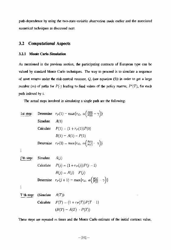
32.1 Monte Carlo Simulation

As mentioned in the previous section, the participating contracts of European type can be

valued by standard Monte Carlo techniques. The way to proceed is to simulate a sequence

of asset returns under the risk-neutral measure, Q, (see equation (5)) in order to get a large

number (m) of paths for P(.) leading to final values of the policy reserve, P”(T), for each

path indexed by i.

The actual steps involved in simulating a single path are the following:

1st step: Determine rp(l) = max{rc, o (g -1))

Simulate 41)

Calculate P(1) = (1+ ~P(l))P(O)

B(1) = A(1) - P(1)

Determine rp(2) = max{rG, o($$ - r)}

j’th step; Simulate A(j)

Calculate P(j) = (1 + TP(j))P(j - 1)

B(j) = 4) - P(j)

Determine rp(j + 1) = max(r0, o (3 -7))

T’th step: (Simulate A(T))

Calculate P(T) = (1+ rp(T))P(T - 1)

(B(T) = A(T) - P(T))

These steps are repeated m times and the Monte Carlo estimate of the initial contract value,

241-

vE(0), is found by averaging the P’(T)‘s and discounting back to time zero, i.e.

(16)

The standard error of the Monte Carlo estimate is obtained as an easy by-product of the

simulation run and is given by

with obvious notation.

There are a number of methods for enhancing the precision of the Monte Carlo estimates

and in our implementation we have employed one of the simplest - the antithetic variable

technique, which is described in e.g. Hull (1997). The reader is also referred to the pioneering

article by Boyle (1977) the recent survey by Boyle, Broadie, and Glasserman (1997), and the

excellent book by Gentle (1998) for further details and more advanced techniques.

The simulation framework is also well-suited for the analysis of issues such as optimal

reserving, the distribution of the future solvency degree, and default probabilities at the in-

dividual contract level. We take a brief look at some of these issues in section 4 where our

numerical work is presented and discussed.

We finally report some technical details in relation to the simulation experiments. Firstly,

in generating the necessary sequence of random numbers we employed the multiplicative con-

gnrential generator supplied with Borland’s Delphi Pascal 4.0 (for details on random number

generators, see e.g. Press et al. (1989) and Gentle (1998)). This particular random number

generator has a period which exceeds 2s1. The sequence was initialized and shuffled (to elim-

inate sequential correlation) according to the Bays and Durham algorithm described in Press

et al. (1989) p, 215-216. The uniform variates were transformed to independent normal vari-

ates using the Box-Muller transformation (see e.g. Quandt (1983)). All Monte Carlo results

reported are based on the same 1,000,000 simulation runs, i.e. on the same sequence of gen-

erated random variates. This permits a more direct comparison between the various contracts

without having to allow for random differences in simulated conditions. The values of the

-242-

European participating contracts reported in Tables 2, 3, and 4 below have been obtained in

this way.

3.2.2 The Recursive Binomial Method

In order to be able to price the American participating contracts we have also implemented

a binomial tree model a la Cox, Ross, and Rubinstein (1979). The European contracts can

also be priced by using this methodology and excluding early exercise so this technique also

conveniently provides us with a rough check on the vahres obtained via Monte Carlo simulation,

cf. earlier.

Because of the dependence of the contract values on both A(.) and P(.) we are forced to

implement a recursive scheme that keeps track of these variates at all knots in the tree starting

from time zero. More specifically, we have used T time steps - typically 20. This allows

for T + 1 final values of A(T), 2T different paths, and similarly (up to) 2T different terminal

values of P(T).

The prices of the American participating policies reported in Tables 2 and 3 have all been

obtained using this methodology.

4 Numerical Results

In this section we present results from the numerical analysis of the model. We first report and

discuss the valuation results in relation to the participating European as well as the American

contracts. We then perform a numerical study of default probabilities on an individual contract

level which is in line with traditional reserving analyses.

The results of the pricing analysis are contained in Tables 2-4 where we study contracts

for which Pa = 100, Ba = 0, T = 20 years and rg = 4.5%. In Table 2, the volatility of the

reference portfolio is set to 15%t9 whereas u = 30% in Table 3. The riskless interest rate is

chosen from the set {8.0%, 6.0%, 4.0%). The distribution rate, o, and the target buffer ratio,

19Pennacchi and Lewis (1994) estimate the average volatility of pension assets to about 15%. See also the discussion in Kaka and Jain (1997).

-243-

y, are varied within each panel in the tables.

There are two values in each entry of Tables 2 and 3. The fist is the value of the European

contract obtained by Monte Carlo simulation as explained earlier. The value of the otherwise

equivalent American-type policy is given in parentheses below the European price. These

prices are obtained via the recursive binomial method discussed earlietZO

In the interpretation of the tables, recall that (Y = 0 corresponds to the extreme situation

where surplus is never distributed and the value of -y is redundant. The policyholder receives

TG per year for the entire period of the contract which has thus effectively degenerated into a

20 year zero-coupon bond. The present value of this bond is given as e@’ . PO . (1 + T(G)"' in

the top row of each of the three panels in Tables 2 and 3. This value is ‘clean’ in the sense that

it does not contain any contribution from bonus or surrender options, and it will obviously be

below par when the market interest rate is high relative to the guaranteed interest rate and vice

versa. Note that (Y = 0 and European contract values below par imply that American contract

values are precisely at par indicating that these contracts should be terminated immediately.

The above-mentioned bond element is present in all prices but when CY > 0 there will also

be a contribution to the contract value from the bonus option. A large o obviously implies a

more favorable bonus option, ceteris paribus, so contract values ate rising in (Y. Conversely,

an increase in the target buffer ratio, 7, means less favorable terms for the option elements,

so contract values decrease as y increases. Hence, bonus policies with relatively low QS and

high ys can be classified as conservative whereas contracts with the opposite characteristics

can be labelled aggressive. In this connection it should be recalled that y = 0.00 corresponds

to the situation where the life insurance company does not aim at building reserves.

Another conclusion is immediate from Tables 2 and 3. It can be seen that constructing par

contracts (&, = 100) is a matter of extreme sensitivity to the distribution policy parameters y

and CL This aspect is further illustrated in Table 4, where the contract values from-Tables 2

and 3 have been decomposed into their basic components, i.e. the risk free bond element, the

*“In a few cases where early exercise is never optimal (Atom panel of Table 2) we obtained values of the American contracts which were slightly lower (less than 1%) than those of their European counterparts. This is due to discretization err01 in the binomial approach so in these cases we have relied upon sod reported the values obtained by Monte Carlo simulation also for the American contracts.

-244-

bonus option and the surrender option.

In the tables we see that the American contracts are always more valuable than their

European counterparts, the difference being the value of the surrender option. Also as expected,

contract values increase as the bonus policy moves from conservative towards more aggressive.

However, note that the value of the surrender option decreases with a more aggressive bonus

policy. This is quite intuitive since a more aggressive bonus policy is purely to the advantage

of the policyholder. Consequently, his incentive to exercise prematurely may be partly or fully

removed in this way.

When the risk free interest rate drops towards and perhaps below the guaranteed interest

rate, the contract value increases although the value of the option elements decreases. This is

explained by the fact that the interest rate guarantee itself moves from being in a sense our of

rhe money to being at or in the money. Being in effect a riskless bond, this contract element

of course rises in value when the market interest rate drops. Note at the same time that the

value of the surrender option decreases as staying in the company becomes more attractive

the closer the riskless rate is to the guaranteed interest rate. In other words, the incentive to

exercise prematurely will gradually disappear as the market interest rate drops.

The effect of the level of volatility of the underlying portfoho can be seen from comparing

Tables 2 and 3. As is usual, option elements become more valuable with increasing uncertainty.

We do not report valuation results for non-zero initial values of the buffer. It is quite clear,

however, that if for example Bt, > 0, the contract values shown in the tables would increase

since surplus obtained over the contracts’ life would not have to be partly used to build up and

maintain the target buffer. Finally, in each panel we indicate the average relative standard

error of the 24 prices obtained by Monte Carlo simulation. The individual standard errors

(not reported) are calculated as the standard error of the Monte Carlo estimate divided by the

price estimate itself.

-245-

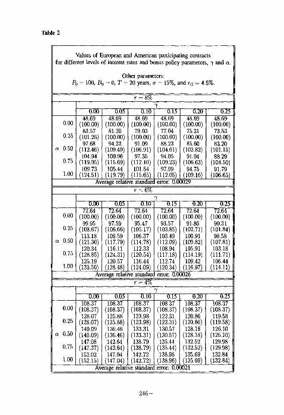
Table 2

Value.~ of European and American participating contracts for different levels of interest rates and bonus policy parameters, y and CL

Other parameters: p0 = 100, B,, = 0, T = 20 years, u = 15%, and T[; = 4.5%.

T = 8%

-246-

'Fable 3

Values of European and American participating contracts for different levels of interest rates and bonus policy parameters, y and o.

Other parameters: 8, = 100, Bt, = 0, T = 20 years, (r = 30%, and T(: = 4.5%.

T = 8% Y

7 0. 0.

0.00 (po8d6090) (l%%) (l%E) (l%%) (l%%) (l%!E) 104.07 101.63 99.35 97.24 95.26 93.41

0.25 (126.76) (124.32) (122.00) (119.99) (WiL;;) (;;Mi;) 127.26 123.42 119.89 116.62

@ 0.56 (152.62) (148.48) (144.61) (141.02) (137.72) (134.91)

0.75 (::;:;i) ($Z) $2;) (Ei$ (::E:) (:2:~0’) 150.56 145.40 140.67 136.34 132.34 128.66

1.00 (180.46) ( 174.43) (168.84) (163.63) (158.82) (154.35) Average relative standard error: 0.06089

T = 6%

T = 4%

Average relative standard error: 0.00066

-247

Table 4

Decomposition of Participating European and American Contract Values Pa = 100, Ba = 0, T = 20 years, c = 15%, and rG = 4.5%.

a Conservative scenario with (Y = 0.00.

’ Neutral scenario with Q = 0.25 and y = 0.15.

’ Aggressive scenario with (Y = 1.00 and y = 0.00.

In order to provide a different perspective on the implications of the model, we have ex-

tended the simulation analysis to cover an issue of relevance to the reserving process. Specif-

ically, we have estimated by simulation the probability of default on the individual contract

for various bonus policy parameters. The probabilities reported are risk neutral, i.e. they are

Q-probabilities. These differ from the true probabilities (P-probabilities) to the extent that the

expected return on assets differ from the risk free rate of interest. We note that to obtain default

probabilities under the P-measure would be computationally equivalent but would require a

subjective choice of the value of the parameter p in equation (2).

We consider European contracts only and Table 5 below contains the estimated default

probabilities where default is defined as the event that B(T) < 0. The top panel represents

the base case where we have taken T(; = 4.5%,~ = S%, Bt, = 0, and 17 = 15%. Different

bonus policies are studied by varying (Y and y as in our earlier pricing analysis. These parame-

-248-

ters are seen to represent a rather risky regime for the insurance company: default probabilities

vary between 0.23 and 0.68. The following three panels each depicts a situation where we

have changed one, and only one, parameter from the base case in a favorable direction as seen

from the side of the company. First, the volatility of assets was lowered to 10%. Second, the

guaranteed interest rate was lowered to 2.5%, and third, the initial reserve, Bo, was set to 20.

In the fifth panel all three changes were applied simultaneously.

‘able 5

Default probabilities for Participating European Contracts

PO = 100, T = 20 years, and T = 8%.

0.00 0.05 0.10 ?0.15 0.20 0.25 0.00 0.23 0.23 0.23 0.23 0.23 0.23

(r = 15% 0.25 0.37 0.34 0.32 0.31 0.29 0.28 TG = 4.5% CY 0.50 0.52 0.47 0.43 0.40 0.37 0.35 B,, = 0 0.75 0.62 0.56 0.51 0.46 0.43 0.39

1.00 0.68 0.62 0.57 0.51 0.47 0.43

The change in volatility from 15% to 10% in the second panel is seen to be quite effectful. For

what we consider to be realistic values of the bonus policy parameters, the default probability

is more than cut in half. As seen from the third panel, the effect on default probabilities of

a lowering of the guaranteed interest rate can also be dramatic, whereas for this particular

choice of parameters the impact of an initial buffer of substantial size is not that significant

(fourth panel). Of course, when the effects are combined as in the fifth panel, the default

probabilities can be made quite small. This is particularly outspoken when bonus policies are

in the conservative to moderate area.

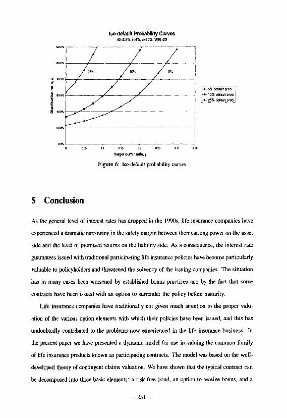
An alternative view on default probabilities is given in Figures 5 and 6 where we have

drawn iso-default probability curves, i.e. curves depicting combinations of o and -y which

result in the same default probabilities for an otherwise given set of parameters. Figure 5 uses

parameters as in the base case in Table 5 and thus represents a problematic situation where the

company must set a very conservative bonus policy to ensure default probabilities below 25%.

Figure 6, on the other hand, represents a relatively safe scenario corresponding to the fifth

panel in Table 5 where the company would have to specify a very aggressive bonus policy in

order to experience default probabilities in excess of 25%.

Isodefault Prob&illty Curves ffi45%, r=o%.a=l6%, a(O@

25% j

oI6 0, 015 02 025 03 035 Taqel bdkr ratio, 7

Figure 5: Iso-defauh probability curves

-250

Isodefaull Probability Curves rG=L5X,r=a%,o=lo%,B(opo

Figure 6: I-default probability curves

5 Conclusion

As the general level of interest rates has dropped in the l!?!Ns, life insurance companies have

experienced a dramatic narrowing in the safety margin between their earning power on the asset

side and the level of promised returns on the liability side. As a consequence, the interest rate

guarantees issued with traditional participating life insurance policies have become particularly

valuable to policyholders and threatened the solvency of the issuing companies. The situation

has in many cases been worsened by established bonus practices and by the fact that some

contracts have been issued with an option to surrender the policy before maturity.

Life insurance companies have traditionally not given much attention to the proper valu-

ation of the various option elements with which their policies have been issued, and this has

undoubtedly contributed to the problems now experienced in the life insurance business. In

the present paper we have presented a dynamic model for use in valuing the common family

of life insurance products known as participating contracts. The model was based on the well-

developed theory of contingent claims valuation. We have shown that the typical contract can

be decomposed into three basic elements: a risk free bond, an option to receive bonus, and a

-251-

surrender option.

The properties of the model were explored numerically. The analysis showed that contract

values are highly dependent on the assumed bonus policy and on the spread between the

market interest rate and the guaranteed rate of interest built into the contract. In another

application of the model, we estimated by simulation the relation between bonus policies

and the probability of default at the individual contract level. This analysis showed default

probabilities of substantial size for realistic parameter choices indicating that the management

of the life insurance company should take solvency problems very seriously. In this respect,

initiatives on both the asset and the liability sides could be considered. An obvious first

choice could be to reduce asset volatility by changing the asset composition towards less risky

assets. But andher potential problem enters here. The return offered by less risky assets

(bonds) might be so low that such a move would only make it certain that interest guarantees

could not be honored in the future. A classical asset substitution problem where the company

management is forced into taking risks might thus exist. Alternatively, to reduce the probability

of default, the company could consider more conservative bonus policies to the extent that this

is permitted by law and the contractual terms. In fact, the possibility for the management to

change the bonus policy parameters in a sense constitutes a counter option which we have not

explicitly taken into account in this paper. This is an interesting subject for future research

as would be the analysis of how the asset mix could possibly be optimally described as a

function of the liability situation of the life insurance company.

Some other natural paths for further research emerge. In the present article, a model was

constructed in order to describe actual insurance company behavior with particular respect to

applied accounting principles and bonus policies. Future research should try to establish the

ideal way in the sense that systematic market value accounting should constitute the basis of

the balance sheet as well as the bonus policy. Furthermore, realism could obviously be added

to the model by considering periodic premiums and taking into account mortality, lapses and

various expense charges. Lastly, an interesting issue would be to incorporate the possibility

of default of the life insurance company and to analyze how this would affect contract values

and possibly also the optimal surrender strategy.

-252-

References

Albizzati, M.-O. and H. Geman (1994): “Interest Rate Risk Management and Valuation of the

Surrender Option in Life Insurance Policies,” Journal of Risk and Insurance, 61(4):616-637.

Babbel, D. F. and C. Merrill (1999): “Economic Valuation Models for Insurers,” North

American Actuarial Journal. Forthcoming.

Baccinello, A. R. and E Grtu (1993a): “Pricing Equity-Linked Life Insurance with Endoge-

nous Minimum Guarantees,” Insurance: Mathematics and Economics, 12(3):245-2X

(1993b): “Pricing Equity-Linked Life Insurance with Endogenous Minimum

Guarantees: A Corrigendum,” Insurance: Mathematics and Economics, 13:303-304.

Bilodeau, C. (1997): “Better Late than Never: The Case of the Rollover Option,” Insurance:

Mathematics and Economics, 21:103-111.

Black, E and M. Scholes (1973): “The Pricing of Options and Corporate Liabilities,” Journal

of Political Economy, 81(3):637-654.

Black, K. and H. D. Skipper (1994): Life Insurance, Prentice Hall, Englewood Cliffs, NJ,

USA, twelfth edition.

Boyle, P P (1977): “Options: A Monte Carlo Approach,” Journal of Financial Economics,

4:323-338.

Boyle, P P., M. Broadie, and P. Glasserman (1997): “Monte Carlo Methods for Security

Pricing,” Journal of Economic Dynamics and Control, 21:1267-1321.

Boyle, P P and M. R. Hardy (1997): “Reserving for Maturity Guarantees: Two Approaches,”

Insurance: Mathematics and Economics, 21: 113-127.

Boyle, P. P and E. S. Schwartz (1977): “Equilibrium Prices of Guarantees under Equity-

Linked Contracts,” Journal of Risk and Insurance, 441639-660.

-253-

Brennan, M. J. (1993): “Aspects of Insurance, Intermediation and Finance,” The Geneva

Papers on Risk and Insurance Theory, 18( 1):7-30.

Brennau, M. J. and E. S. Schwartz (1976): “The Pricing of Equity-Linked Life Insurance

Policies with an Asset Value Guarantee,” Journal of Financial Economics, 3:195-213.

(1979): “Alternative Investment Strategies for the Issuers of Equity Linked Life

Insurance Policies with an Asset Value Guarantee,” Journal of Business, 52( 1):63-93.

Briys, E. and F. de Varenne (1997): “On the Risk of Life Insurance Liabilities: Debunking

Some Common Pitfalls,” Journal of Risk and Insurance, 64(4):673-694.

Broadie, M. and P. Glasserman (1997): “Pricing American-style Securities Using Simula-

tion,” Journal of Economic Dynamics and Control, 21:1323-1352.

Cox, J. C., S. A. Ross, and M. Rubinstein (1979): “Option Pricing: A Simplified Approach,”

Journal of Financial Economics, 7:229-263.

Embrechts, P. (1996): “Actuarial versus Financial Pricing of Insurance,” Working Paper,

Wharton Financial Institutions Center, WP 96-17.

Gentle, J. E. (1998): Random Number Generation and Monte Carlo Methods, Springer-

Verlag, New York.

Grosen, A. and P L. Jorgensen (1997): “Valuation of Early Exercisable Interest Rate Guar-

antees,” Journal of Risk and Insurance, 64(3):481-503.

Harrison, M. J. and D. M. Kreps (1979): “Martingales and Arbitrage in Multipetiod Securities

Markets,” Journal of Economic Theory, 20:38 l-408.

Hull, J. C. (1997): Options, Futures, and other Derivatives, Prentice-Hall, Inc., 3rd edition.

Kalra, R. and G. Jain (1997): “A Continuous-time Model to Determine the Intervention

Policy for PBGC,” Journal of Banking and Finance, 21: 1159-l 177.

254-

Karatzas, I. (1988): “On the Pricing of the American Option,” Applied Mathematics and

Optimization, 17:37-60.

Lewis, C. M. and G. G. Pennacchi (1997): “Valuing Insurance for Defined-Benefit Pension

Plans,” Working Paper.

Maturity Guarantees Working Party (1980): “Report,” Journal of fhe Institute of Actuaries,

107:103-209.

Miltersen, K. R. and S.-A. Persson (1997): “Pricing Rate of Return Guarantees in a Heath-

Jarrow-Morton Framework,” Working Paper, Odense University.

(1998): “Guaranteed Investment Contracts: Distributed and Undistributed Ex-

cess Return,” Working Paper, Odense University.

Nielsen, J. A. and K. Sandmann (1995): ‘Equity-Linked Life Insurance: A Model with

Stochastic Interest Rates,” Insurance: Mathematics and Economics, 16:225-253.

Nielsen, J. P and H. L. Thaning (1996): “Matching of Assets and Liabilities in Danish

Pension Companies,” Working Paper, PFA Pension and Copenhagen Business School.

Pennacchi, G. and C. Lewis (1994): “The Value of Pension Benefit Guaranty Corporation

Insurance,” Journal of Money, Credit and Banking, 26:735-753.

Persson, S.-A. and K. K. Aase (1997): “Valuation of the Minimum Guaranteed Return

Embedded in Life Insurance Products,” Journal of Risk and Insurance, 64(4):599-617.

Press, W. H., B. P. Flannery, S. A. Teukolsky, and W. T. Vetterling (1989): Numerical

Recipes in Pascal, Cambridge University Press.

Quandt, R. (1983): “Computational Problems and Methods,” in Griliches, Z. and M.

Intriligator, editors, Handbook of Econometrics, volume 1, chapter 12. North-Holland.

The Danish Financial Supervisory Authority (1998): Rapport om betaling for rentegaranti

(Report on the Payment for Interest Rate Guarantees), FinanstilsynetfThe Danish Financial

-255-

Supervisory Authority. The report (in Danish) and an English summary are available at the

internet address ‘www.ftnet.dk’.

Tilley, J. (1993): “Valuing American Options in a Path Simulation Model,” Transactions of

the Society of Actuaries, 45233-104.

Vanderhoof, I. T. and E. I. Altman, editors (1998): The Fair Value of Insurance Liabilities,

Kluwer Academic Publishers. The New York University Salomon Center Series on Financial

Markets and Institutions.

-256-