Fan Cooling at High Altitude - epac-inc.com Cooling at High Altitude.pdf · When the altitude is increased, the air density is decreased and therefore, the weight flow is decreased

Copyright ©EPAC-INC.COM FOR MORE INFORMATION, VISIT OUR WEB SITE: EPAC-INC.COM Tel: (603) 533-9011

EPAC Software COLDPLATE Report

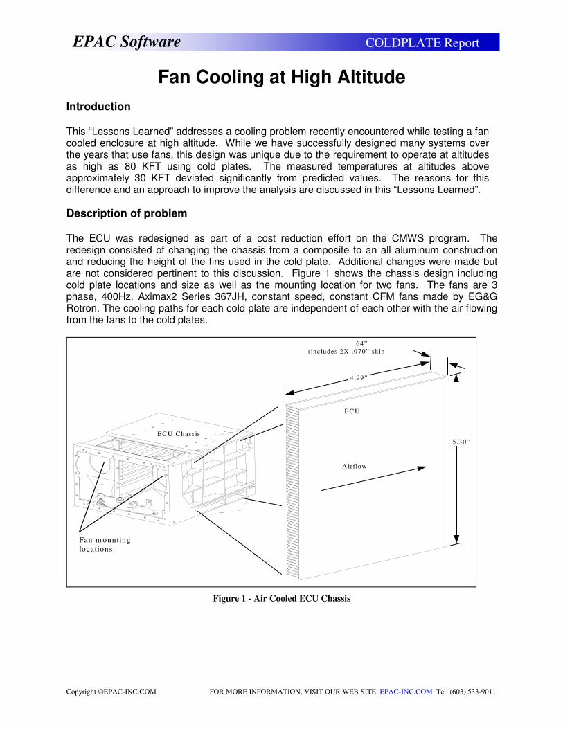
Fan Cooling at High Altitude Introduction This “Lessons Learned” addresses a cooling problem recently encountered while testing a fan cooled enclosure at high altitude. While we have successfully designed many systems over the years that use fans, this design was unique due to the requirement to operate at altitudes as high as 80 KFT using cold plates. The measured temperatures at altitudes above approximately 30 KFT deviated significantly from predicted values. The reasons for this difference and an approach to improve the analysis are discussed in this “Lessons Learned”.

Description of problem The ECU was redesigned as part of a cost reduction effort on the CMWS program. The redesign consisted of changing the chassis from a composite to an all aluminum construction and reducing the height of the fins used in the cold plate. Additional changes were made but are not considered pertinent to this discussion. Figure 1 shows the chassis design including cold plate locations and size as well as the mounting location for two fans. The fans are 3 phase, 400Hz, Aximax2 Series 367JH, constant speed, constant CFM fans made by EG&G Rotron. The cooling paths for each cold plate are independent of each other with the air flowing from the fans to the cold plates.

4.99”

.64”

(inc ludes 2X .070” skin

thickness)

5.30”

A irflow

D irection

EC U C hass is

EC U

C O LD PLA T E

Fan m ounting

locations

Figure 1 - Air Cooled ECU Chassis



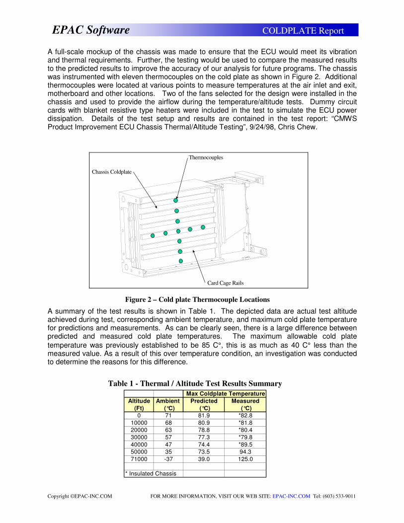
A full-scale mockup of the chassis was made to ensure that the ECU would meet its vibration and thermal requirements. Further, the testing would be used to compare the measured results to the predicted results to improve the accuracy of our analysis for future programs. The chassis was instrumented with eleven thermocouples on the cold plate as shown in Figure 2. Additional thermocouples were located at various points to measure temperatures at the air inlet and exit, motherboard and other locations. Two of the fans selected for the design were installed in the chassis and used to provide the airflow during the temperature/altitude tests. Dummy circuit cards with blanket resistive type heaters were included in the test to simulate the ECU power dissipation. Details of the test setup and results are contained in the test report: “CMWS Product Improvement ECU Chassis Thermal/Altitude Testing”, 9/24/98, Chris Chew.

A summary of the test results is shown in Table 1. The depicted data are actual test altitude achieved during test, corresponding ambient temperature, and maximum cold plate temperature for predictions and measurements. As can be clearly seen, there is a large difference between predicted and measured cold plate temperatures. The maximum allowable cold plate

temperature was previously established to be 85 C°, this is as much as 40 C° less than the measured value. As a result of this over temperature condition, an investigation was conducted to determine the reasons for this difference.

Chassis Coldplate

Thermocouples

Card Cage Rails

Figure 2 – Cold plate Thermocouple Locations

Table 1 - Thermal / Altitude Test Results Summary

Max Coldplate Temperature

Altitude Ambient Predicted Measured

(Ft) (°C) (°C) (°C)

0 71 81.9 *82.8

10000 68 80.9 *81.8

20000 63 78.8 *80.4

30000 57 77.3 *79.8

40000 47 74.4 *89.5

50000 35 73.5 94.3

71000 -37 39.0 125.0

* Insulated Chassis



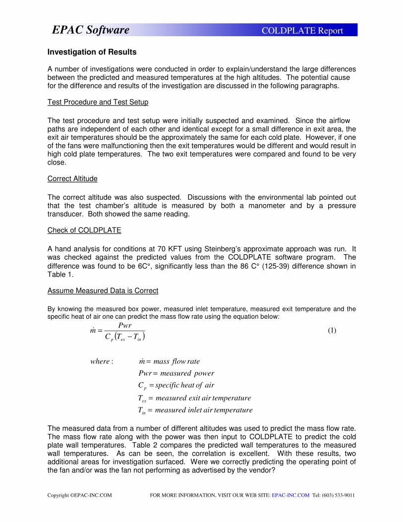
Investigation of Results A number of investigations were conducted in order to explain/understand the large differences between the predicted and measured temperatures at the high altitudes. The potential cause for the difference and results of the investigation are discussed in the following paragraphs.

Test Procedure and Test Setup

The test procedure and test setup were initially suspected and examined. Since the airflow paths are independent of each other and identical except for a small difference in exit area, the exit air temperatures should be the approximately the same for each cold plate. However, if one of the fans were malfunctioning then the exit temperatures would be different and would result in high cold plate temperatures. The two exit temperatures were compared and found to be very close.

Correct Altitude

The correct altitude was also suspected. Discussions with the environmental lab pointed out that the test chamber’s altitude is measured by both a manometer and by a pressure transducer. Both showed the same reading.

Check of COLDPLATE

A hand analysis for conditions at 70 KFT using Steinberg’s approximate approach was run. It was checked against the predicted values from the COLDPLATE software program. The

difference was found to be 6C°, significantly less than the 86 C° (125-39) difference shown in Table 1.

Assume Measured Data is Correct

By knowing the measured box power, measured inlet temperature, measured exit temperature and the specific heat of air one can predict the mass flow rate using the equation below:

( )

etemperaturairinletmeasuredT

etemperaturairexitmeasuredT

airofheatspecificC

powermeasuredPwr

rateflowmassmwhere

TTC

Pwrm

in

ex

p

inexp

=

=

=

=

=

−=

&

&

:

)1(

The measured data from a number of different altitudes was used to predict the mass flow rate. The mass flow rate along with the power was then input to COLDPLATE to predict the cold plate wall temperatures. Table 2 compares the predicted wall temperatures to the measured wall temperatures. As can be seen, the correlation is excellent. With these results, two additional areas for investigation surfaced. Were we correctly predicting the operating point of the fan and/or was the fan not performing as advertised by the vendor?



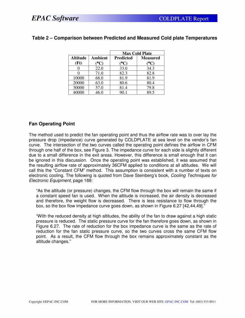
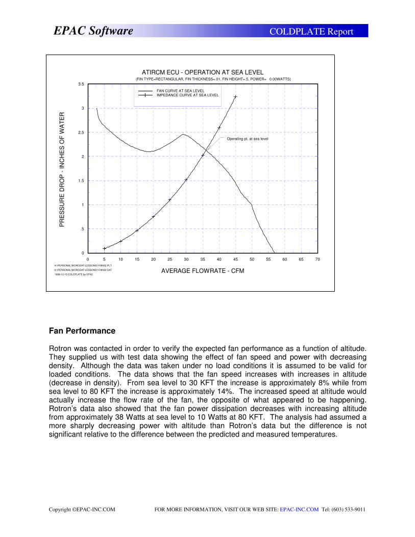
Fan Operating Point

The method used to predict the fan operating point and thus the airflow rate was to over lay the pressure drop (impedance) curve generated by COLDPLATE at sea level on the vendor’s fan curve. The intersection of the two curves called the operating point defines the airflow in CFM through one half of the box, see Figure 3. The impedance curve for each side is slightly different due to a small difference in the exit areas. However, this difference is small enough that it can be ignored in this discussion. Once the operating point was established, it was assumed that the resulting airflow rate of approximately 36CFM applied to conditions at all altitudes. We will call this the “Constant CFM” method. This assumption is consistent with a number of texts on electronic cooling. The following is quoted from Dave Steinberg’s book, Cooling Techniques for Electronic Equipment, page 188:

“As the altitude (or pressure) changes, the CFM flow through the box will remain the same if a constant speed fan is used. When the altitude is increased, the air density is decreased and therefore, the weight flow is decreased. There is less resistance to flow through the box, so the box flow impedance curve goes down, as shown in Figure 6.27 [42,44,49].” “With the reduced density at high altitudes, the ability of the fan to draw against a high static pressure is reduced. The static pressure curve for the fan therefore goes down, as shown in Figure 6.27. The rate of reduction for the box impedance curve is the same as the rate of reduction for the fan static pressure curve, so the two curves cross the same CFM flow point. As a result, the CFM flow through the box remains approximately constant as the altitude changes.”

Max Cold Plate Altitude

(Ft)

Ambient

(°°°°C)

Predicted

(°°°°C)

Measured

(°°°°C)

0 22.0 33.0 34.3 0 71.0 82.3 82.8

10000 68.0 81.9 81.9 20000 63.0 80.6 80.4 30000 57.0 81.4 79.8 40000 46.0 90.1 89.5

Table 2 – Comparison between Predicted and Measured Cold plate Temperatures



Fan Performance Rotron was contacted in order to verify the expected fan performance as a function of altitude. They supplied us with test data showing the effect of fan speed and power with decreasing density. Although the data was taken under no load conditions it is assumed to be valid for loaded conditions. The data shows that the fan speed increases with increases in altitude (decrease in density). From sea level to 30 KFT the increase is approximately 8% while from sea level to 80 KFT the increase is approximately 14%. The increased speed at altitude would actually increase the flow rate of the fan, the opposite of what appeared to be happening. Rotron’s data also showed that the fan power dissipation decreases with increasing altitude from approximately 38 Watts at sea level to 10 Watts at 80 KFT. The analysis had assumed a more sharply decreasing power with altitude than Rotron’s data but the difference is not significant relative to the difference between the predicted and measured temperatures.

AVERAGE FLOWRATE - CFM

0 5 10 15 20 25 30 35 40 45 50 55 60 65 70

PR

ES

SU

RE

DR

OP

- I

NC

HE

S O

F W

AT

ER

0

.5

1

1.5

2

2.5

3

3.5

ATIRCM ECU - OPERATION AT SEA LEVEL (FIN TYPE=RECTANGULAR, FIN THICKNESS=.01, FIN HEIGHT=.5, POWER= 0.00WATTS)

1998-12-15 COLDPLATE by EPAC

H:\PERSONAL\WORDDAT\LESSONS1\FANS2.DAT

H:\PERSONAL\WORDDAT\LESSONS1\FANS2.PLT

FAN CURVE AT SEA LEVELIMPEDANCE CURVE AT SEA LEVEL

Operating pt. at sea level

Figure 3 – Fan Operating Point at Sea Level



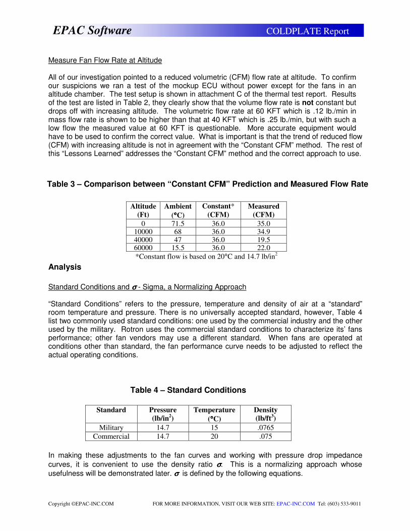
Measure Fan Flow Rate at Altitude All of our investigation pointed to a reduced volumetric (CFM) flow rate at altitude. To confirm our suspicions we ran a test of the mockup ECU without power except for the fans in an altitude chamber. The test setup is shown in attachment C of the thermal test report. Results of the test are listed in Table 2, they clearly show that the volume flow rate is not constant but drops off with increasing altitude. The volumetric flow rate at 60 KFT which is .12 lb./min in mass flow rate is shown to be higher than that at 40 KFT which is .25 lb./min, but with such a low flow the measured value at 60 KFT is questionable. More accurate equipment would have to be used to confirm the correct value. What is important is that the trend of reduced flow (CFM) with increasing altitude is not in agreement with the “Constant CFM” method. The rest of this “Lessons Learned” addresses the “Constant CFM” method and the correct approach to use.

Analysis

Standard Conditions and σσσσ - Sigma, a Normalizing Approach “Standard Conditions” refers to the pressure, temperature and density of air at a “standard” room temperature and pressure. There is no universally accepted standard, however, Table 4 list two commonly used standard conditions: one used by the commercial industry and the other used by the military. Rotron uses the commercial standard conditions to characterize its’ fans performance; other fan vendors may use a different standard. When fans are operated at conditions other than standard, the fan performance curve needs to be adjusted to reflect the actual operating conditions.

In making these adjustments to the fan curves and working with pressure drop impedance

curves, it is convenient to use the density ratio σσσσ. This is a normalizing approach whose

usefulness will be demonstrated later. σσσσ is defined by the following equations.

Altitude

(Ft)

Ambient

(°°°°C)

Constant*

(CFM)

Measured

(CFM)

0 71.5 36.0 35.0 10000 68 36.0 34.9 40000 47 36.0 19.5 60000 15.5 36.0 22.0

*Constant flow is based on 20°C and 14.7 lb/in2

Table 3 – Comparison between “Constant CFM” Prediction and Measured Flow Rate

Table 4 – Standard Conditions

Standard Pressure

(lb/in2)

Temperature

(°°°°C)

Density

(lb/ft3)

Military 14.7 15 .0765

Commercial 14.7 20 .075



conditiondardtannonsoraltitudeatetemperaturT

airforttanconsgasR

conditiondardtannonsoraltitudeatpressureP

RT

Paltitudeatdensity

conditionsdardtansatdensitywhere

ALT

ALT

ALT

ALTALT

STD

STD

ALT

=

=

=

==

=

=

)3(

:

(2)

ρ

ρ

ρ

ρσ

Fan Laws

The fan laws, which are taken from the Rotron catalog and listed below, characterize the behavior of fans due to changes in air density, size and speed.

conditionsdifferentatvaluestheareand

ndissipatiopowerPwr

density

droppressureP

fantheofdiametersizephysicalSIZE

fantheofspeedN

rateflowvolumetheQwhere

SIZE

SIZE

N

N

SIZE

SIZE

N

NPP

SIZE

SIZE

N

NQQ

21

=

=

=∆

=

=

=

=

∆=∆

=

ρ

ρ

ρ

ρ

ρ

)(

)6( PwrPwr

)5(

)4(

5

1

2

3

1

2

1

212

2

1

2

2

1

2

1

212

3

1

2

1

212

From equation (4) it can be seen that for a fixed fan, the flow rate is directly proportional to the fan speed, thus if there is a 10% increase in speed there will be a 10% increase in volume flow rate. Equation (5) shows that the pressure drop is directly proportional to the density for a fixed constant speed fan. This means that the fan curve for different altitudes can be determined by

multiplying the pressure drop at each point by the density ratio i.e. σ. By combining equation (4) and (5), the pressure drop in terms of density and volume flow rate is determined as shown below.

)7(

4

2

1

2

1

2

1

212

∆=∆

SIZE

SIZE

Q

QPP

ρ

ρ



The importance of this relationship is that in order for the “Constant CFM” method to be valid the box impedance curve must also be proportional to the density and the square of the volume flow rate. If this is the case then the operating point (intersection of the fan and impedance curve) will remain the same. The next paragraphs demonstrate this relationship and what happens if the impedance curve is not proportional to the density and the square of the volume flow rate.

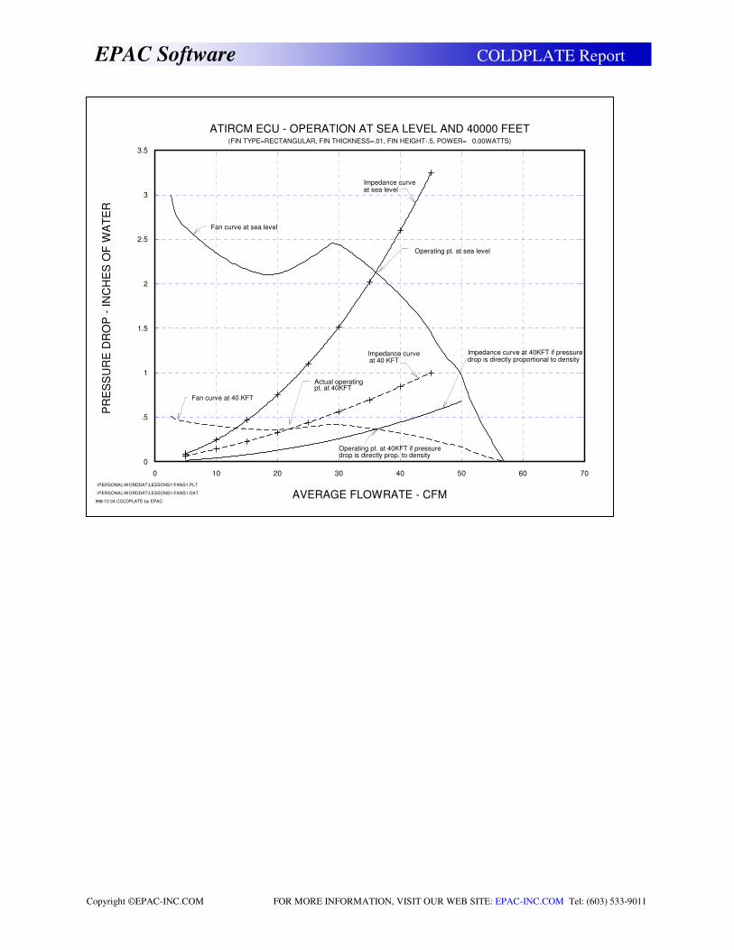
Fan Performance at Altitude

Starting with Figure 3, three additional curves were added to examine fan performance at altitude. First a fan curve at 40 KFT was added. The curve was modified from the fan curve at sea level (standard conditions) by multiplying the pressure drop at each point times the density

ratio σσσσ. Second, an impedance curve using the temperature and pressure at 40 KFT was generated by COLDPLATE and added to the plot. Lastly, the impedance curve at sea level was

multiplied by the density ratio σσσσ at 40 KFT; this represents the impedance curve that would follow the “Constant CFM” method. Figure 4 shows all of the curves on a single plot. The intersection of the sea level fan curve and the sea level impedance curve is approximately 36 CFM as is the intersection of the 40 KFT fan curve and the 40 KFT “Constant CFM” curve. However, the intersection of the 40 KFT fan curve and the 40 KFT COLDPLATE generated impedance curve is not the same, it is approximately 22 CFM. This value is very close to 19.5 CFM, the measured value shown in Table 3. The difference in predicted flow rates further demonstrates that the “Constant CFM” method is not correct for all cases and shows what the correct approach should be. The next section goes into the equations used to predict the box impedance and shows details of why the “Constant CFM” method is in general not correct.



Figure 4 –Fan Operation at Sea Level and 40 KFT

AVERAGE FLOWRATE - CFM

0 10 20 30 40 50 60 70

PR

ES

SU

RE

DR

OP

- I

NC

HE

S O

F W

AT

ER

0

.5

1

1.5

2

2.5

3

3.5

ATIRCM ECU - OPERATION AT SEA LEVEL AND 40000 FEET(FIN TYPE=RECTANGULAR, FIN THICKNESS=.01, FIN HEIGHT-.5, POWER= 0.00WATTS)


H:\PERSONAL\WORDDAT\LESSONS1\FANS1.DAT

H:\PERSONAL\WORDDAT\LESSONS1\FANS1.PLT

Operating pt. at sea level

Impedance curve at 40KFT if pressuredrop is directly proportional to density

Actual operatingpt. at 40KFT

Operating pt. at 40KFT if pressuredrop is directly prop. to density

Impedance curveat 40 KFT

Impedance curveat sea level

Fan curve at sea level

Fan curve at 40 KFT



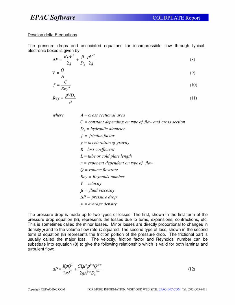
Develop delta P equations

The pressure drops and associated equations for incompressible flow through typical electronic boxes is given by:

densityaverage

droppressureP

viscosity fluid=

velocityV

numberReynolds'=Rey

rateflowvolumeQ

flow of type on dependent exponent=n

lengthplatecoldortubeL

tcoefficienlossK

gravityofonacceleratig

factorfrictionf

diameterhydraulicD

sectioncrossandflowoftypeondependingnstantcoC

areal sectionacrossAwhere

VD=Rey

Rey

Cf

A

QV

g

V

D

fL

g

VKP

h

h

n

h

=

=∆

=

=

=

=

=

=

=

=

=

=

=

+=∆

ρ

µ

µ

ρ

ρρ

)11(

)10(

)9(

)8(22

22

The pressure drop is made up to two types of losses. The first, shown in the first term of the pressure drop equation (8), represents the losses due to turns, expansions, contractions, etc. This is sometimes called the minor losses. Minor losses are directly proportional to changes in

density ρρρρ and to the volume flow rate Q squared. The second type of loss, shown in the second term of equation (8) represents the friction portion of the pressure drop. The frictional part is usually called the major loss. The velocity, friction factor and Reynolds’ number can be substitute into equation (8) to give the following relationship which is valid for both laminar and turbulent flow:

)12(22 12

21

2

2

n

h

n

nnn

DgA

QCL

gA

QKP

+−

−−

+=∆ρµρ



The first term of (12) indicates that similar to the fan pressure drop equation (7), the pressure drop is directly proportional to the density and the square of the volume flow rate. From the second term of (12) it can be seen that only if n is equal to 2 and if the viscosity is a constant would this similarity exist. Therefore, in general, the frictional part of the pressure drop is not directly proportional to the density ρ and to the volume flow rate squared, thus changes in altitude (or changes from standard conditions) will result in changes in volume flow rate. The friction relationship for both laminar and turbulent flow is next examined in detail.

Laminar Flow

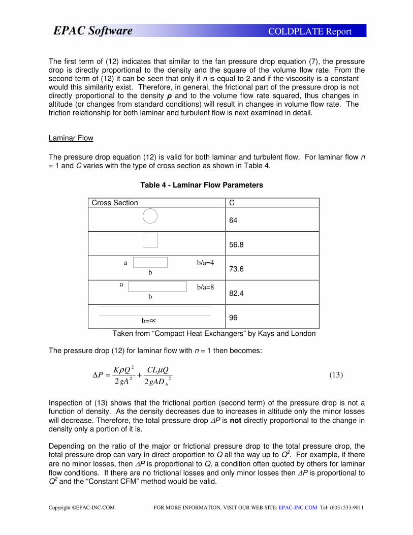
The pressure drop equation (12) is valid for both laminar and turbulent flow. For laminar flow n = 1 and C varies with the type of cross section as shown in Table 4.

The pressure drop (12) for laminar flow with n = 1 then becomes:

)13(22

22

2

hgAD

QCL

gA

QKP

µρ+=∆

Inspection of (13) shows that the frictional portion (second term) of the pressure drop is not a function of density. As the density decreases due to increases in altitude only the minor losses

will decrease. Therefore, the total pressure drop ∆P is not directly proportional to the change in density only a portion of it is. Depending on the ratio of the major or frictional pressure drop to the total pressure drop, the total pressure drop can vary in direct proportion to Q all the way up to Q2. For example, if there

are no minor losses, then ∆P is proportional to Q, a condition often quoted by others for laminar

flow conditions. If there are no frictional losses and only minor losses then ∆P is proportional to Q2 and the “Constant CFM” method would be valid.

Table 4 - Laminar Flow Parameters

Cross Section C

64

56.8

73.6

82.4

96

Taken from “Compact Heat Exchangers” by Kays and London

a

a

b

b

b=∝

b/a=4

b/a=8



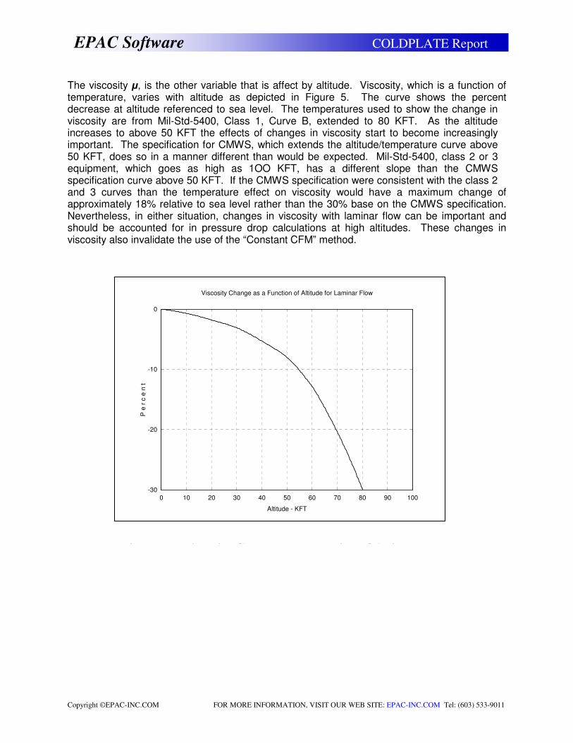
The viscosity µ, is the other variable that is affect by altitude. Viscosity, which is a function of temperature, varies with altitude as depicted in Figure 5. The curve shows the percent decrease at altitude referenced to sea level. The temperatures used to show the change in viscosity are from Mil-Std-5400, Class 1, Curve B, extended to 80 KFT. As the altitude increases to above 50 KFT the effects of changes in viscosity start to become increasingly important. The specification for CMWS, which extends the altitude/temperature curve above 50 KFT, does so in a manner different than would be expected. Mil-Std-5400, class 2 or 3 equipment, which goes as high as 1OO KFT, has a different slope than the CMWS specification curve above 50 KFT. If the CMWS specification were consistent with the class 2 and 3 curves than the temperature effect on viscosity would have a maximum change of approximately 18% relative to sea level rather than the 30% base on the CMWS specification. Nevertheless, in either situation, changes in viscosity with laminar flow can be important and should be accounted for in pressure drop calculations at high altitudes. These changes in viscosity also invalidate the use of the “Constant CFM” method.

Altitude - KFT

0 10 20 30 40 50 60 70 80 90 100

P e

r c

e n

t

-30

-20

-10

0

Viscosity Change as a Function of Altitude for Laminar Flow

Figure 5 – Viscosity Change as a Function of Altitude



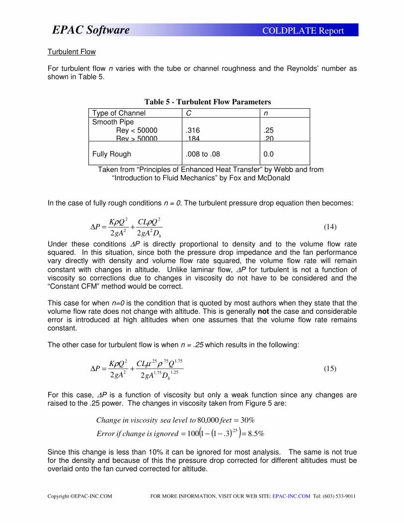
Turbulent Flow For turbulent flow n varies with the tube or channel roughness and the Reynolds’ number as shown in Table 5.

In the case of fully rough conditions n = 0. The turbulent pressure drop equation then becomes:

)14(22 2

2

2

2

hDgA

QCL

gA

QKP

ρρ+=∆

Under these conditions ∆P is directly proportional to density and to the volume flow rate squared. In this situation, since both the pressure drop impedance and the fan performance vary directly with density and volume flow rate squared, the volume flow rate will remain

constant with changes in altitude. Unlike laminar flow, ∆P for turbulent is not a function of viscosity so corrections due to changes in viscosity do not have to be considered and the “Constant CFM” method would be correct. This case for when n=0 is the condition that is quoted by most authors when they state that the volume flow rate does not change with altitude. This is generally not the case and considerable error is introduced at high altitudes when one assumes that the volume flow rate remains constant. The other case for turbulent flow is when n = .25 which results in the following:

)15(22 25.175.1

75.175.25.

2

2

hDgA

QCL

gA

QKP

ρµρ+=∆

For this case, ∆P is a function of viscosity but only a weak function since any changes are raised to the .25 power. The changes in viscosity taken from Figure 5 are:

( )( ) %5.83.11100

%30000,80

25.=−−=

=

ignoredischangeifError

feettolevelseaitycosvisinChange

Since this change is less than 10% it can be ignored for most analysis. The same is not true for the density and because of this the pressure drop corrected for different altitudes must be overlaid onto the fan curved corrected for altitude.

Table 5 - Turbulent Flow Parameters

Type of Channel C n

Smooth Pipe Rey < 50000 Rey > 50000

.316 .184

.25 .20

Fully Rough

.008 to .08

0.0

Taken from “Principles of Enhanced Heat Transfer” by Webb and from “Introduction to Fluid Mechanics” by Fox and McDonald



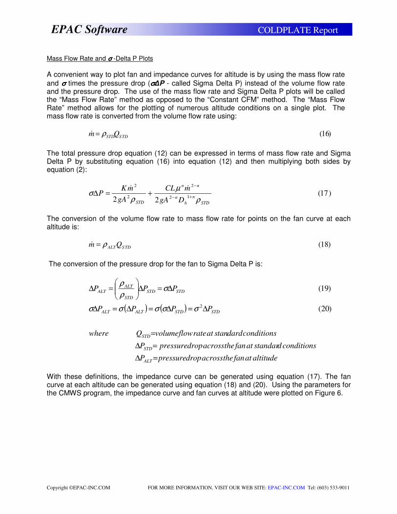
Mass Flow Rate and σσσσ -Delta P Plots

A convenient way to plot fan and impedance curves for altitude is by using the mass flow rate

and σσσσ times the pressure drop (σσσσ∆P - called Sigma Delta P) instead of the volume flow rate and the pressure drop. The use of the mass flow rate and Sigma Delta P plots will be called the “Mass Flow Rate” method as opposed to the “Constant CFM” method. The “Mass Flow Rate” method allows for the plotting of numerous altitude conditions on a single plot. The mass flow rate is converted from the volume flow rate using:

)16(TDSSTDQm ρ=&

The total pressure drop equation (12) can be expressed in terms of mass flow rate and Sigma Delta P by substituting equation (16) into equation (12) and then multiplying both sides by equation (2):

)17(22

12

2

2

2

STD

n

h

n

nn

STD DgA

mCL

gA

mKP

ρ

µ

ρσ

+−

−

+=∆&&

The conversion of the volume flow rate to mass flow rate for points on the fan curve at each altitude is:

)18(TDSALTQm ρ=&

The conversion of the pressure drop for the fan to Sigma Delta P is:

( ) ( )

altitudeatfantheacrossdroppressureP

conditionsdstandaratfantheacrossdroppressureP

conditionsdardtansatrateflowvolumeQwhere

PPPP

PPP

ALT

STD

STD

STDSTDALTALT

STDSTD

STD

ALTALT

=∆

=∆

=

∆=∆=∆=∆

∆=∆

=∆

)20(

)19(

2σσσσσ

σρ

ρ

With these definitions, the impedance curve can be generated using equation (17). The fan curve at each altitude can be generated using equation (18) and (20). Using the parameters for the CMWS program, the impedance curve and fan curves at altitude were plotted on Figure 6.



A number of observations can be made about Figure 6. The format of this type of plot allows one to determine the flow rate at each altitude all within one plot, the intersection of the “Predicted Impedance Curve” and the fan curve at each altitude determine the flow rate at each altitude. Over laid on the figure are what the impedance curve would look like if the flow were either “Fully Laminar” or “Fully turbulent”. The laminar curve has a slope of 1.0 and starts at point where Sigma Delta P is 1. The turbulent curve has a slope of 2, intersects the fan curves at the same relative point at each altitude and represents the “Constant CFM” method. As the altitude increases the observed difference between using the “Constant CFM” method and the “Mass Flow Rate” method becomes dramatic, this also was verified by our test results. The last observation from Figure 6 is that the assumption is almost always made that the Sigma Delta P curve has a constant slope, as can be seen from the figure the slope at sea level is approximately 1.8 while at altitudes above 50 KFT the slope is approximately 1.0.

4 6 8 10-2

2 4 6 8 10-1

2 4 6 8 100

2 4

FLOWRATE - LB/MIN

10-3

2

4

6

810

-210

2

4

6

810

-110

2

4

6

810

010

2

SIG

MA

DE

LT

A P

- IN

CH

ES

OF

WA

TE

RLAMINAR, TURBULENT AND PREDICTED IMPEDANCE CURVES

SIGMA DELTA P VS FLOWRATE(STD PRESS= 14.70PSI, STD TEMP= 21.10C, FIN TYPE=RECTANGULAR, FIN THICKNESS=.010IN, FIN HT=.5, 12FPI, POWER=74.20WATTS)


H:\PERSONAL\WORDDAT\LESSONS1\SUMMARY2.DAT

H:\PERSONAL\WORDDAT\LESSONS1\SUMMARY2.plt

Sea Level, Sigma=.85

40KFT, Sigma=.171

50KFT, Sigma=.109

60KFT, Sigma=.0725

80KFT, Sigma=.0366

Predicted impedance curve

Fully laminar, slope = 1.0

Fully turbulent, slope = 2.0(Constant CFM)

Figure 6 - Mass Flow Rate and σσσσ -Delta P Plot



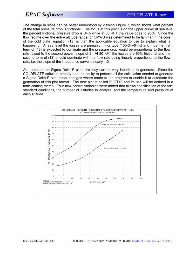
The change in slope can be better understood by viewing Figure 7, which shows what percent of the total pressure drop is frictional. The focus at this point is on the upper curve; at sea level the percent frictional pressure drop is 34% while at 80 KFT the value goes to 95%. Since the flow regime over the entire altitude range for CMWS was determined to be laminar in the core of the cold plate, equation (13) is then the applicable equation to use to explain what is happening. At sea level the losses are primarily minor type (100-34=64%) and thus the first term of (13) is expected to dominate and the pressure drop would be proportional to the flow rate raised to the second power, slope of 2. At 80 KFT the losses are 95% frictional and the second term of (13) should dominate with the flow rate being linearly proportional to the flow rate, i.e. the slope of the impedance curve is nearly 1.0. As useful as the Sigma Delta P plots are they can be very laborious to generate. Since the COLDPLATE software already had the ability to perform all the calculation needed to generate a Sigma Delta P plot, minor changes where made to the program to enable it to automate the generation of this plot format. The new plot is called PLOT18 and its use will be defined in a forth-coming memo. Four new control variables were added that allows specification of the fan: standard conditions, the number of altitudes to analyze, and the temperature and pressure at each altitude.

ALTITUDE, KFT

0 10 20 30 40 50 60 70 80 90 100

% F

RIC

TIO

NA

L P

RE

SS

UR

E D

RO

P

0

10

20

30

40

50

60

70

80

90

100

ATIRCM ECU - PERCENT FRICTIONAL PRESSURE DROP VS ALTITUDE(FLOW IS LAMINAR OVER ENTIRE RANGE)

1999-01-06

H:\PERSONAL\WORDDAT\LESSONS1\DP-F1.DAT

H:\PERSONAL\WORDDAT\LESSONS1\DP-F1.plt

Fin Ht= .5in , Fin Density= 12 Fins/inch

Fin Ht= 1.0in, Fin density= 8 Fins/inch

Figure 7 – Frictional Pressure Drop as a Function of



Corrections to Fan and Impedance Curves There are a number of corrections to the predicted flow rate that may have to be considered or included to arrive at the final predicted flow rate:

• Fan speed

• Viscosity

• Box power

• Fan power

• Radiation

• External convection

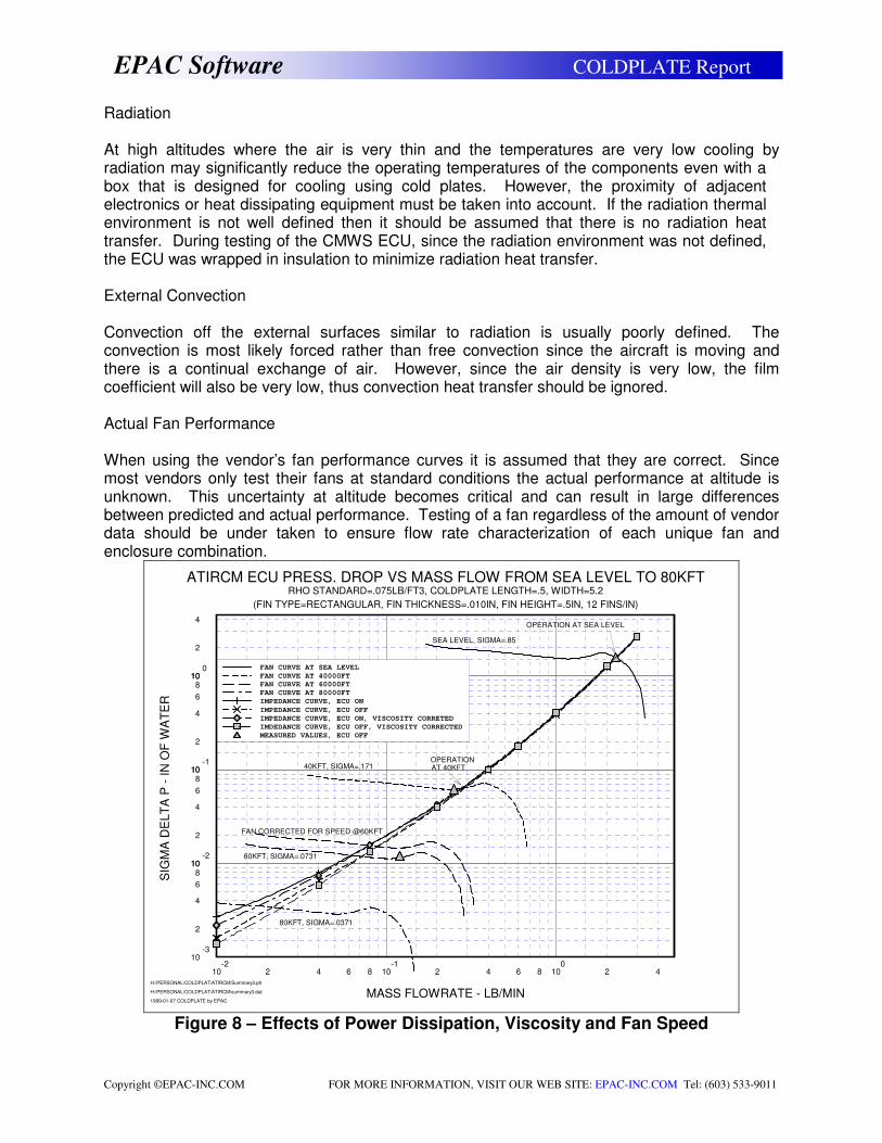
• Actual fan performance Fan Speed Although constant speed fans are advertised as running at constant speed they usually do run faster as the density decreases. As previous mention, the Rotron fan ran as much as 14% faster at reduced density. The fan curve can be corrected to account for this change by using equation (4) and (5). The flow rate is increased by the ratio of the fan speeds while the pressure drop is increased by the ratio squared. The effect of the increased fan speed can be seen in Figure 8 where the fan curve at 60 KFT has been corrected for speed. This correction results in an approximate increase in flow rate of 30%. Viscosity Viscosity effects have been previously discussed, however; the effect of changes in viscosity is demonstrated in Figure 8. At 80 KFT the effect results in an increase of approximately 10%. Viewed from an overall perspective, these viscosity changes can be ignored which will result in a slightly more conservative design. Box Power Power dissipation of electronics within the chassis results in heating of the air that in turn results in a decrease in air density. With decreased density, the mass flow rate through the box decreases. Turning to Figure 8 again, it can be seen that the mass flow rate decreases by 28% at 80 KFT and 14% at 60 KFT. Since this effect can be significant, caution is advised at very high altitudes to be sure that both analysis and testing be done with box power on in determining flow rate. Fan Power With a fan at the inlet to the box, the fan power dissipation can have a similar but smaller effect as the box power dissipation since the air is heated up as it passes over the fan. Additionally, a correction in fan power must be considered since the fan power changes as predicted by the third of the fan laws, equation (6). By equation (6), the fan power should be significantly less at altitude than at sea level since its power is proportional to the change in density and the density changes significantly with altitude. The power is also proportional to the fan speed cubed, however; the change in density dominates any change in fan speed. The Rotron power dissipation data for the CMWS fan did not show as dramatic a decrease in power as predicted by equation (6), in this case the vendor’s data should be used.



Radiation At high altitudes where the air is very thin and the temperatures are very low cooling by radiation may significantly reduce the operating temperatures of the components even with a box that is designed for cooling using cold plates. However, the proximity of adjacent electronics or heat dissipating equipment must be taken into account. If the radiation thermal environment is not well defined then it should be assumed that there is no radiation heat transfer. During testing of the CMWS ECU, since the radiation environment was not defined, the ECU was wrapped in insulation to minimize radiation heat transfer. External Convection Convection off the external surfaces similar to radiation is usually poorly defined. The convection is most likely forced rather than free convection since the aircraft is moving and there is a continual exchange of air. However, since the air density is very low, the film coefficient will also be very low, thus convection heat transfer should be ignored. Actual Fan Performance When using the vendor’s fan performance curves it is assumed that they are correct. Since most vendors only test their fans at standard conditions the actual performance at altitude is unknown. This uncertainty at altitude becomes critical and can result in large differences between predicted and actual performance. Testing of a fan regardless of the amount of vendor data should be under taken to ensure flow rate characterization of each unique fan and enclosure combination.

10-2

2 4 6 8 10-1

2 4 6 8 100

2 4

MASS FLOWRATE - LB/MIN

10-3

2

4

6

810

-210

2

4

6

810

-110

2

4

6

810

010

2

4

SIG

MA

DE

LT

A P

- I

N O

F W

AT

ER

ATIRCM ECU PRESS. DROP VS MASS FLOW FROM SEA LEVEL TO 80KFTRHO STANDARD=.075LB/FT3, COLDPLATE LENGTH=.5, WIDTH=5.2

(FIN TYPE=RECTANGULAR, FIN THICKNESS=.010IN, FIN HEIGHT=.5IN, 12 FINS/IN)


H:\PERSONAL\COLDPLAT\ATIRCM\summary3.dat

H:\PERSONAL\COLDPLAT\ATIRCM\Summary3.plt

FAN CURVE AT SEA LEVEL

FAN CURVE AT 40000FT



IMPEDANCE CURVE, ECU ON

IMPEDANCE CURVE, ECU OFF

IMPEDANCE CURVE, ECU ON, VISCOSITY CORRETED

IMDEDANCE CURVE, ECU OFF, VISCOSITY CORRECTED

MEASURED VALUES, ECU OFF

OPERATION AT SEA LEVEL

OPERATIONAT 40KFT

SEA LEVEL, SIGMA=.85

40KFT, SIGMA=.171

60KFT, SIGMA=.0731

80KFT, SIGMA=.0371

FAN CORRECTED FOR SPEED @60KFT

Figure 8 – Effects of Power Dissipation, Viscosity and Fan Speed



Measured Fan Flow Rate at Altitude - Revisited The tested data in Table 3 was plotted on Figure 8 to show the difference between the “Mass Flow Rate” analysis approach and test data. At both sea level and 40 KFT the correlation is excellent while at 60 KFT the predicted flow rate is approximately 50% of the measured flow rate. As previously discussed, the accuracy of the measurements at 60 KFT are questionable. What is important is that the “Mass Flow Rate” method is a much better predictor of the flow rate than the “Constant CFM” method.

Redesign The measured cold plate temperatures in Table 1 indicate that the as tested fan and cold plate

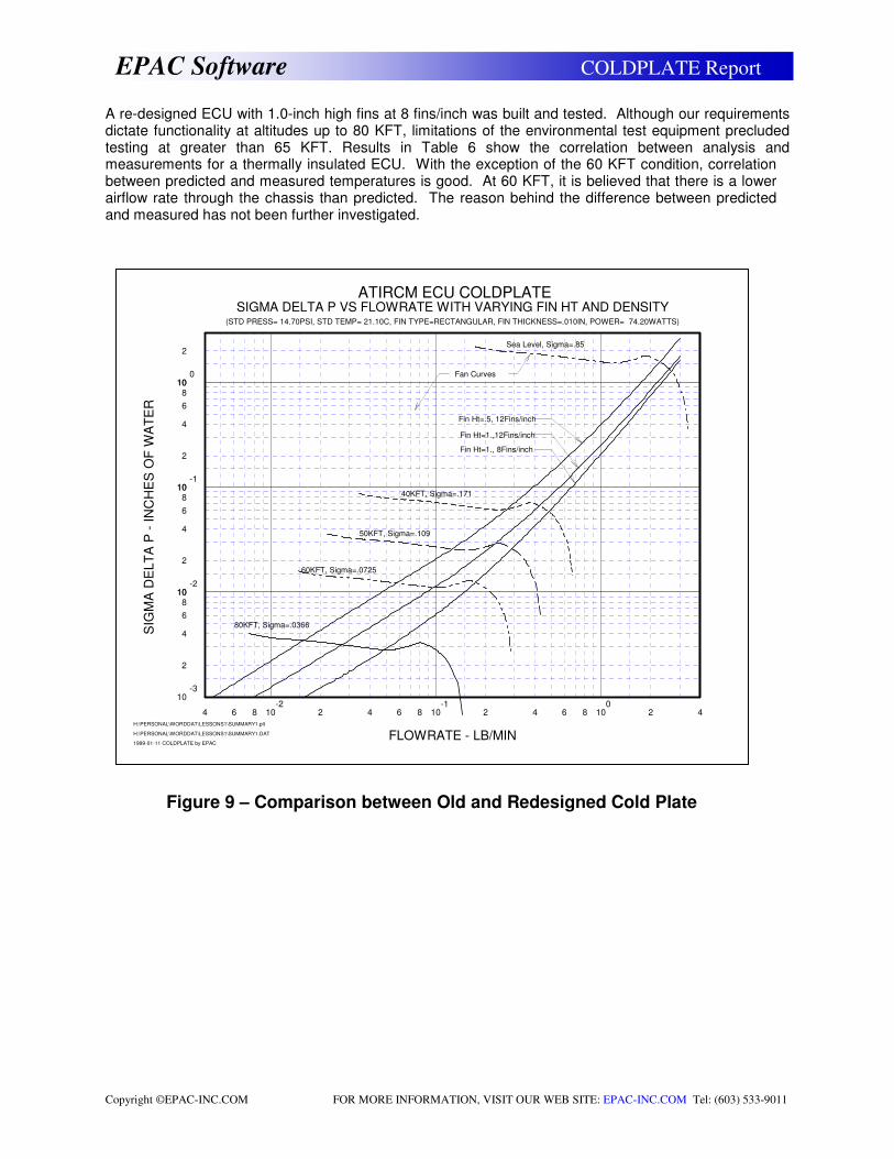
combination would not meet the 85 C° maximum allowable cold plate requirement. Some of the options considered to reduce the temperatures are as follows. Search for another fan that would provide increased flow capability. This was unsuccessful, the current fan was already a high-speed fan running at 20,000 RPM and there was not enough space for a larger fan. Variable speed fans were looked at but their performance at sea level was not acceptable. Reversing the flow direction was considered in order to take out the added air temperature rise due to the fan power dissipation. However, this was not an acceptable for the ECU because the air is heated up by the electronics prior to reaching the fan, which reduces the density thereby reducing the mass flow rate through the box resulting in a net increase in cold plate temperature. Tests run with the fan reversed also showed that the pressure drop was higher in the reverse direction compared to the forward direction. Reversing the air direction would have required a change in the specification; changing the specification was considered an unacceptable approach by the program office. Testing of the ECU was performed at an early enough stage in the design process of the program to allow for redesign of the cold plate. In addition, due to heritage reasons the sidewalls of the ECU enclosure had room to increase the fin height of the cold plate. A number of trade studies were performed to look at increased fin heights and fin densities to optimize the temperature and pressure drop to redesign the cold plates. The new design chosen was 1.0-inch high fins at 8 fins/inch. Figure 9 shows the amount of improvement in flow rate from the original design of .5-inch high fins at 12 fins/inch to the new configuration. The change in design allowed the flow rate to increase by 15% at sea level to 230% at 80 KFT. Increasing the fin height increases the surface area, which reduces the temperature; reducing the fin density increases the hydraulic diameter, which decreases the friction factor which in turn reduces the pressure drop thus increasing the flow rate. The overall effect from the pressure drop prospective is the frictional part of the pressure drop is decreased at all altitudes as witnessed by Figure 7.



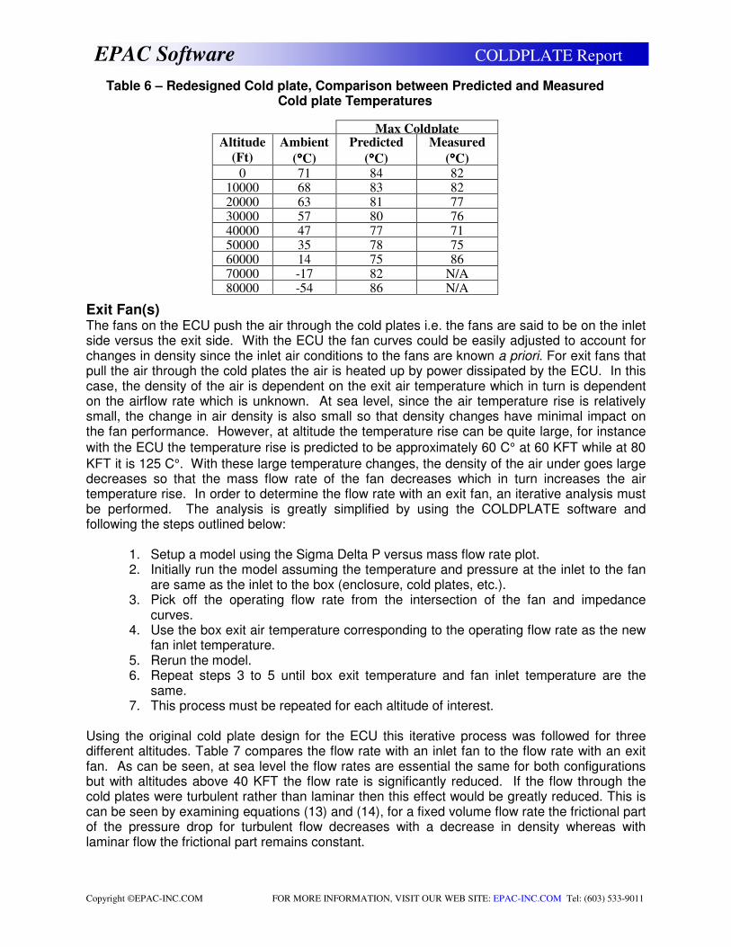
A re-designed ECU with 1.0-inch high fins at 8 fins/inch was built and tested. Although our requirements dictate functionality at altitudes up to 80 KFT, limitations of the environmental test equipment precluded testing at greater than 65 KFT. Results in Table 6 show the correlation between analysis and measurements for a thermally insulated ECU. With the exception of the 60 KFT condition, correlation between predicted and measured temperatures is good. At 60 KFT, it is believed that there is a lower airflow rate through the chassis than predicted. The reason behind the difference between predicted and measured has not been further investigated.

4 6 8 10-2

2 4 6 8 10-1

2 4 6 8 100

2 4

FLOWRATE - LB/MIN

10-3

2

4

6

810

-210

2

4

6

810

-110

2

4

6

810

010

2

SIG

MA

DE

LT

A P

- I

NC

HE

S O

F W

AT

ER

ATIRCM ECU COLDPLATESIGMA DELTA P VS FLOWRATE WITH VARYING FIN HT AND DENSITY

(STD PRESS= 14.70PSI, STD TEMP= 21.10C, FIN TYPE=RECTANGULAR, FIN THICKNESS=.010IN, POWER= 74.20WATTS)


H:\PERSONAL\WORDDAT\LESSONS1\SUMMARY1.DAT

H:\PERSONAL\WORDDAT\LESSONS1\SUMMARY1.plt

Sea Level, Sigma=.85

40KFT, Sigma=.171

50KFT, Sigma=.109

60KFT, Sigma=.0725

80KFT, Sigma=.0366

Fin Ht=.5, 12Fins/inch

Fin Ht=1.,12Fins/inch

Fin Ht=1., 8Fins/inch

Fan Curves

Figure 9 – Comparison between Old and Redesigned Cold Plate



Exit Fan(s) The fans on the ECU push the air through the cold plates i.e. the fans are said to be on the inlet side versus the exit side. With the ECU the fan curves could be easily adjusted to account for changes in density since the inlet air conditions to the fans are known a priori. For exit fans that pull the air through the cold plates the air is heated up by power dissipated by the ECU. In this case, the density of the air is dependent on the exit air temperature which in turn is dependent on the airflow rate which is unknown. At sea level, since the air temperature rise is relatively small, the change in air density is also small so that density changes have minimal impact on the fan performance. However, at altitude the temperature rise can be quite large, for instance

with the ECU the temperature rise is predicted to be approximately 60 C° at 60 KFT while at 80

KFT it is 125 C°. With these large temperature changes, the density of the air under goes large decreases so that the mass flow rate of the fan decreases which in turn increases the air temperature rise. In order to determine the flow rate with an exit fan, an iterative analysis must be performed. The analysis is greatly simplified by using the COLDPLATE software and following the steps outlined below:

1. Setup a model using the Sigma Delta P versus mass flow rate plot. 2. Initially run the model assuming the temperature and pressure at the inlet to the fan

are same as the inlet to the box (enclosure, cold plates, etc.). 3. Pick off the operating flow rate from the intersection of the fan and impedance

curves. 4. Use the box exit air temperature corresponding to the operating flow rate as the new

fan inlet temperature. 5. Rerun the model. 6. Repeat steps 3 to 5 until box exit temperature and fan inlet temperature are the

same. 7. This process must be repeated for each altitude of interest.

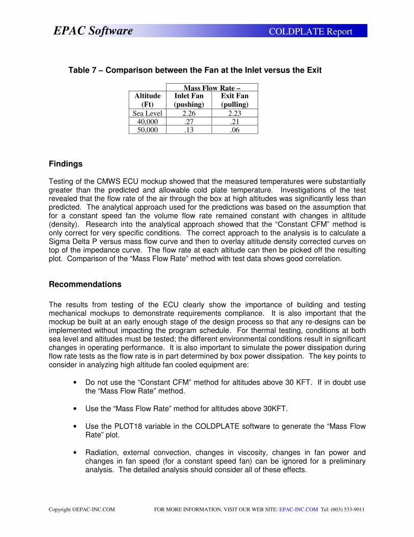
Using the original cold plate design for the ECU this iterative process was followed for three different altitudes. Table 7 compares the flow rate with an inlet fan to the flow rate with an exit fan. As can be seen, at sea level the flow rates are essential the same for both configurations but with altitudes above 40 KFT the flow rate is significantly reduced. If the flow through the cold plates were turbulent rather than laminar then this effect would be greatly reduced. This is can be seen by examining equations (13) and (14), for a fixed volume flow rate the frictional part of the pressure drop for turbulent flow decreases with a decrease in density whereas with laminar flow the frictional part remains constant.

Max Coldplate Altitude

(Ft)

Ambient

(°°°°C)

Predicted

(°°°°C)

Measured

(°°°°C) 0 71 84 82

10000 68 83 82 20000 63 81 77 30000 57 80 76 40000 47 77 71 50000 35 78 75 60000 14 75 86 70000 -17 82 N/A 80000 -54 86 N/A

Table 6 – Redesigned Cold plate, Comparison between Predicted and Measured Cold plate Temperatures



Findings Testing of the CMWS ECU mockup showed that the measured temperatures were substantially greater than the predicted and allowable cold plate temperature. Investigations of the test revealed that the flow rate of the air through the box at high altitudes was significantly less than predicted. The analytical approach used for the predictions was based on the assumption that for a constant speed fan the volume flow rate remained constant with changes in altitude (density). Research into the analytical approach showed that the “Constant CFM” method is only correct for very specific conditions. The correct approach to the analysis is to calculate a Sigma Delta P versus mass flow curve and then to overlay altitude density corrected curves on top of the impedance curve. The flow rate at each altitude can then be picked off the resulting plot. Comparison of the “Mass Flow Rate” method with test data shows good correlation.

Recommendations

The results from testing of the ECU clearly show the importance of building and testing mechanical mockups to demonstrate requirements compliance. It is also important that the mockup be built at an early enough stage of the design process so that any re-designs can be implemented without impacting the program schedule. For thermal testing, conditions at both sea level and altitudes must be tested; the different environmental conditions result in significant changes in operating performance. It is also important to simulate the power dissipation during flow rate tests as the flow rate is in part determined by box power dissipation. The key points to consider in analyzing high altitude fan cooled equipment are:

• Do not use the “Constant CFM” method for altitudes above 30 KFT. If in doubt use the “Mass Flow Rate” method.

• Use the “Mass Flow Rate” method for altitudes above 30KFT.

• Use the PLOT18 variable in the COLDPLATE software to generate the “Mass Flow Rate” plot.

• Radiation, external convection, changes in viscosity, changes in fan power and changes in fan speed (for a constant speed fan) can be ignored for a preliminary analysis. The detailed analysis should consider all of these effects.

Mass Flow Rate – Altitude

(Ft)

Inlet Fan

(pushing)

Exit Fan

(pulling)

Sea Level 2.26 2.23 40,000 .27 .21 50,000 .13 .06

Table 7 – Comparison between the Fan at the Inlet versus the Exit

Documents

Fan Cooling at High Altitude - epac-inc.com Cooling at High Altitude.pdf · When the altitude is increased, the air density is decreased and therefore, the weight flow is decreased