Robust Whole-Body Motion Control of Legged Robots

Farbod Farshidian, Edo Jelavic, Alexander W. Winkler, Jonas Buchli

Abstract— We introduce a robust control architecture forthe whole-body motion control of torque controlled robotswith arms and legs. The method is based on the robustcontrol of contact forces in order to track a planned Centerof Mass trajectory. Its appeal lies in the ability to guaranteerobust stability and performance despite rigid body modelmismatch, actuator dynamics, delays, contact surface stiffness,and unobserved ground profiles. Furthermore, we introduce atask space decomposition approach which removes the couplingeffects between contact force controller and the other non-contact controllers. Finally, we verify our control performanceon a quadruped robot and compare its performance to astandard inverse dynamics approach on hardware.

I. INTRODUCTIONThe robustness of motion controllers for legged robots has

recently attracted a significant research interest. Generallyin any robotic application, a generic motion control requiresthree main components namely, (i) trajectory planning whichis responsible for generating reference trajectories, (ii) a stateobserver to estimate the state of the robot and (iii) a stabi-lizing feedback controller which is responsible for trackingthe reference trajectories and rejecting disturbances. For anysuccessful hardware implementation, the robustness shouldbe considered in designing each of these three modules. Here,we focus on the robustness of the stabilizing controller.

Task space inverse dynamics is a popular approach forwhole–body control of legged robots given that the referencetrajectory has already been calculated [1], [2]. Hierarchicalinverse dynamics based on cascades of quadratic programshas been proposed for the control of legged robots andimplemented on torque controlled legged robots [3], [4].Inverse kinematics based approaches with constraints andhierarchical control approach such as [5] have also been usedfor the control of legged robots. All of these methods are ingeneral a versatile tool for implementing already existingreference trajectories. However, the main limitation of thesemethods is their assumption and reliance on ideal forcetracking actuators. Thus, they are often susceptible to theactuators dynamics, model uncertainties, and delays.

In order to increase the robustness of a motion controller,different schemes have been proposed. A robust inversedynamics method is proposed by [6], [7] which makes thetask constraints less susceptible to the additive uncertaintyin joint torques. In [8], [9], an adaptive control method hasbeen used to estimate or improve the rigid body model inorder to adapt the controller. Task space robustness of ma-nipulator’s motion has been considered by [10], [11] wherethe proposed method guarantees stability in the presence of

∗All authors are with the Agile & Dexterous Robotics Lab, ETH Zurich,Switzerland, email: {farbodf, jelavice, winklera, buchlij}@ethz.ch

rigid body model mismatch and actuator dynamics. Whiletorque control algorithms with high-performance [12] canreinforce the perfect actuator assumption to a certain extent,their performance is still not ideal. In this paper, we propose afeedback control structure which can increase the robustnessof the controller in face of actuator dynamics, finite contactsurface stiffness, and unobserved ground profile. We assumethat the objective of the whole-body stabilizing controller isto track planned trajectories of the Center of Mass (CoM).Considering that the CoM motion is only affected by theexternal forces, a robust implementation of the given plan canbe achieved by robustly controlling the robot’s interactionports (e.g. footsteps or contact forces) with the environment.

The main contributions of this work are as follows: First,we introduce an Internal Model Control (IMC) structure tofeedback control the end-effector (e.g. stance leg) contactforce by considering the actuator dynamics and delays. Then,we demonstrate that we can achieve the robust stability andperformance of our IMC contact force controller with theproper tuning of IMC; the tuning boils down to the selectionof a single parameter. Furthermore, in order to decouplethe contact force controller and the non-contact end-effectorcontroller (e.g. swing leg), we introduce a general approachfor either hierarchical or co-equal task space decompositioninto subsystems. While this approach is formulated for fully-actuated legged robots extension to under-actuated cases isconceivable. Finally, we discuss the experimental results onour quadrupedal robot, HyQ. and compare it to a standardwhole-body control method of legged robot used in [2].

II. BACKGROUND

In this section, we briefly introduce the task space model-ing approach and model-based feedback force control struc-ture which we will use later in our proposed method.

A. Task Space

Assuming rigid body modelling, we can write the equa-tions of motion of a robot as

M(q)q+C(q, q)+G(q) = S>τ +J>c⊥λ c⊥ +J>c‖λ c‖

Jc‖ q = 0, Jc⊥ q = 0, λ⊥ ≥ 0 (1)

where M, C, G, and S are respectively the generalizedinertia matrix, Coriolis-centrifugal forces, generalized gravityforces, and selection matrix. q is the generalized coordi-nate vector which is augmented by the floating base posecoordinate. λ c⊥ and λ c‖ are the orthogonal and tangentialcontact forces. Their corresponding Jacobian are Jc⊥ and Jc‖respectively and the equality and the inequality equations arethe constraints that are introduced through contacts. The task

arX

iv:1

703.

0232

6v1

[cs

.RO

] 7

Mar

201

7

space dynamics can be obtained by mapping the whole-bodymodel in Equation (1) to the range space of the task Jacobianmatrix, Jx, [13]. Thus, we can write

Mx(q)x+Cx(q, q)+Gx(q) = S>x τ +J>c,xλ , (2)

where we have

Mx = J†>x MJ†

x

Cx = J†>x C−MxJxq

Gx = J†>x G

Sx = SJ†x

Jc,x = JcJ†x

J†x = M−1J>x

(JxM−1J>x

)−1(3)

J†x is the dynamically consistent right pseudo-inverse of the

full row rank Jacobian matrix, Jx. In the next section, we usethis equation to derive motion dynamics of three task spacesdefined in our subsystem decomposition approach.

B. Internal Model Control (IMC)

The IMC structure is an alternative parametrization overthe stable classical feedback controllers for linear systems.However, in contrast to the classical approach which usesthe system’s measured outputs for feedback control, IMCdirectly utilizes the system dynamics model for calculatinga feedback signal based on the difference between the mea-sured outputs and the predicted outputs of its internal model(Fig. 2). Moreover, it uses an inverse model approach in orderto improve its tracking and disturbance rejection. Anothermajor advantage of IMC is that it allows a systematictradeoff between performance and robustness [14] since theclosed loop sensitivity function is linear with respect to itscontroller. In the next section, we explain the design processof a robust IMC structure in more details.

To the best of our knowledge, IMC has not been appliedfor task space force control. However, a closely relatedmethod known as disturbance observer (DOB) has beenrecently implemented for force control in low-level controlof actuators [15], [16]. Strictly speaking, IMC and DOB arenot the same. However, they both rely on the internal modelprinciple. The only notable exception for DOB application inrigid body level is [17] in which DOB is used to achieve theprecise tracking on a humanoid arm while being compliant.

III. APPROACH

The main objective of this paper is to increase the ro-bustness of the motion controller for tracking given CoMtrajectories. Based on the Newton-Euler equation of motion,the CoM dynamics are only affected by external forces on therobot. Thus, a robust implementation of a given CoM plancan be achieved by robustly controlling the contact forcesand contact point locations at the moments of touchdown.The robust and compliant control of the free end-effectors(e.g. swing legs and arms) has been extensively studied inthe literature [17]. Therefore, we mainly focus on the robustcontrol of the contact forces. First, we introduce a new con-tact force controller which performs robustly in face of rigidbody model mismatch, actuator dynamics, delays, contactsurface stiffness, and unobserved ground profiles. Then, toreduce the coupling effects between controllers, we propose

Fig. 1. Overview of the model (blue) and control structure (green). Thesystem model is separated into three subsystems, a CoM subsystem, acontact subsystem and a non-contact subsystem. Each of these systems iscontrolled with a corresponding controller. The black triangles describe themappings between subsystem states and generalized coordinates q as wellas between subsystems torques and joint torques τ .

a generalized approach for controlling two task spaces withsimilar precedence. Finally, we explain our control approachfor CoM and non-contact degrees of freedom (DoF).

In our proposed method, the legged robot model is brokendown into three subsystems, namely: contact subsystem,CoM subsystem, and non-contact subsystem as shown inFig. 1 (the blue block). The contact subsystem includesDoF in system which directly manipulate the contact forces.The CoM subsystem is attributed to the whole-body CoMdynamics. At last, the non-contact subsystem comprises ofany remaining DoF such as the swing legs.

A. Contact Force Control at End–Effectors

The contact subsystem is defined in the range space ofthe end-effectors’ Jacobians Jc that are in contact with theenvironment (e.g. stance legs). The equation of motion forthis subsystem has the same form as (2), thus we have

Cc(q, q)+Gc(q) = S>c τ +λ , λ⊥ ≥ 0, (4)

where the end-effector acceleration, xc, is set to zero due tothe equality constraints in Equation (2) for non-slipping con-tact points. Notice that the projected contact forces Jacobianin this equation is an identity matrix since Jc,c = JcJ†

c = I.The assumption that Jc is a full row rank matrix holds aslong as there exist at least three independent DoF for eachcontact point. Furthermore, conveniently all of the contactrelated equality and inequality constraints are assimilated inEquation (4). Assuming that all of the joints are actuated, S>chas the same range space as Jc which renders this subsystemas fully actuated. Therefore, we get

Cc(q, q)+Gc(q) = τc +λ , λ⊥ ≥ 0 (5)

where τc = S>c τ . Notice that the mapping from τc to τ isnot unique since for any given τc, there exists a subspace ofdimension Dim(Ker(Jc)) in the generalized force space thatproduces the same value. Later, we will use this characteristicto decouple the contact and non-contact subsystems.

In order to control this subsystem, we first feedback-linearize its dynamics by setting τc = F+Cc(q, q)+Gc(q).Then, we get

λ =−F, λ⊥ ≥ 0. (6)

According to this equation, the relation between contactforces and F is algebraic. However, this equation is basedon the rigid body modeling and hard contact assumptionand does not consider the actuator dynamics and softness ofthe contact surfaces (xc 6= 0). In order to design a controllerwhich can deal with these issues, we propose a feedbackstructure known as IMC. To guarantee the robustness of thisstructure, we need to make a few assumptions on the systemdynamics and the external signal type (such as referencesand disturbances). First, we assume that all of the actuatorshave the same nominal dynamics. This assumption causesthe projected force τc and consequently F to have the samenominal dynamics as actuators. We use here a first ordersystem with delay (first order deadtime system). Thus, foreach component i, in the contact force vector, we have thefollowing dynamics

Hp(s) =λi

ui=− e−ηds

ηs+1, (7)

where Hp(s) is the nominal model between the ith con-tact force component and the ith element of the projectedfeedback-linearized actuator command ui. ηd and η are thenominal delay and the time constant. In this nominal model,we assume that the system does not have a steady state errorto a constant input (the gain is one) which is the case for idealactuators. Finally, for modeling uncertainties of this model,we assume that the actual transfer function of system, Hp(s),belong to the family Π defined as

Π =

{Hp(s) |

∥∥∥∥Hp( jω)− Hp( jω)

Hp( jω)

∥∥∥∥≤ l(ω)

}(8)

which means that relative error in each frequency is boundedby l(ω). A typical shape of l(ω) can be found in Fig. 3.In practice, we can also assume that l(0) < 1 which isequivalent to say that the constant input to the actuatorsproduces a steady state force output with less than 100%relative tracking error. This is a reasonable assumption formany force controlled robots. The external signals such asthe reference forces and disturbances are assumed to be stepinputs 1. This class of signals can capture the sudden changesin the contact force reference; such changes appear whenestablishing/breaking contacts as well as disturbances suchas slippage of the legs and push forces on the robot’s body.

The proposed IMC structure is depicted in Fig. 2. Sincethere is no interconnection between non-pair inputs andoutputs, we use a single-input single-output (SISO) con-trol structure for each input-output pairs. Our SISO IMCconsists of two controllers, namely the disturbance rejectioncontroller, qd(s), and the reference tracking controller, qr(s).

1Note that any arbitrary signal can be approximated by a finite set ofshifted step functions

The disturbance rejection controller uses the estimated dis-turbance signal d to reject disturbances, d and the referencetracking controller modulates the input signals in order totrack the desired output (refer to Fig. 2).

Both controllers use a notion of the system inverse model(H−1

p (s)) for improving the closed loop force control per-formance. In general, the design process of IMC consists oftwo steps: (i) design an optimal controller for the nominalplant and (ii) detune the nominal control to obtain robustperformance. The first step of the design uses an H2-optimalcontrol method which minimizes the Integral of SquareError (ISE) criterion for the step type input. The latterstep often uses a lowpass filter in order to guarantee robuststability and robust performance. The H2-optimal controllerhas no tracking error since for ISE being finite, the referencetracking error should asymptotically approach zero. The ISEcriterion is defined as:

min‖e|22 =∫

∞

0‖λ (t)−λr(t)‖2

2dt

Based on H2-optimal theorem [14] the optimal controlleris q(s) = (ηs + 1) f (s) for a first order deadtime systemwith step input which is obtained based on the nominalmodel inverse (H−1

p (s)). Here, f (s) is a lowpass filter. Foroptimal solution f (s) should be unity. However, there are twomajor issues with this choice: first, since the degree of thenominator is higher than the degree of the denominator, thiscontroller will not be a causal system. Second, this systemhas a high amplitude in the high frequencies which makesit susceptible to sensory noise and model uncertainty suchas non-stiff ground (which produces high frequency xc). Toovercome these issues we use a lowpass filter with a properstructure. The following theorem states that there exists sucha filter which can guarantee stability and zero tracking errorfor all the system in the family Π.

Theorem 1: Assume l(ω) is continuous and l(0) < 1.Then there exists a lowpass filter f (s) such that the closedloop system is robustly stable for family Π and it tracksasymptotically error-free constant inputs.

Proof: The proof is based on the corollary (4.3-2) andcorollary (4.4-2) in [14] and the assumption l(0)< 1.

In practice, this filer should be designed by using theminimum order lowpass filter which results in a satisfactoryperformance. On the system used in this paper, a first orderlowpass filter with one free parameter η f was enough forrobust stability and performance.

f (s) =1

η f s+1(9)

This parameter can be tuned directly on the hardware, bygradually increasing η f until a satisfactory performance isobtained. Since η f determines the response time of the con-troller, increasing η f reduces the performance of the closedloop system in favour of robustness. In order to analyticallyguarantee the robust performance of the controller for allsystems in the family Π, we need to show that the followingcondition holds for all the frequencies∣∣l(ω) f (iω)

∣∣+ ∣∣(1− e−iηdω f (iω))

w∣∣< 1 (10)

Fig. 2. Overview of the contact force control structure. This controlleruses feedback-linearization, the obtain a linearized plant. This then allowsto use an IMC structure composed of the internal model Hp(s), disturbancerejection controller qd(s), tracking controller qr(s), and output constraintblocks. Note that the hinge-function block (green) appears only in thecontrol loop for orthogonal forces.where w is a weighting used for determining the desiredclosed-loop system’s bandwidth. A typical shape of w−1 canbe found in [14]. In Section IV, we explain a process ofdetermining η f in order to fulfil the robust performancecriterion in Equation (10).

The last but not least advantage of using the IMC struc-ture is that we can optimally and robustly incorporate theinput/output constraints [18]. In the contact force controlcase, we mostly have output constraints such as the unilateralconstraint of orthogonal forces to the contact surface andstiction/friction in the actuators. To this end, we have useda hinge-function block at the output of the nominal modelin order to account for unilateral constraint for orthogonalcontact surfaces. Moreover, to model the stiction/friction ofthe actuators, we use a deadzone block on the estimateddisturbance d signal. The latter can be interpreted as thecase where the small difference between the nominal model’soutput force and the plant’s output force is considered as theactuators’ stiction/friction resisting force. In the next section,we study the coupling effect between the contact subsystemand other remaining DoF and introduce a generalized methodto prevent this cross coupling.

B. Task Space Control Decoupling

Special care should be taken in mapping τc = S>c τ . Thisis because the generalized forces τ are not only manipulatedby the contact subsystem’s controller, but also by the othercontrollers acting on remaining DoF. This can produceundesirable couplings between controllers. In this section,we show how to systematically decouple the controllersfor different DoF. To this end, we break down the leggedrobot model into three subsystems: contact subsystem, CoMsubsystem, and non-contact subsystem as shown in Fig. 1.Since the contact subsystem and its controller structure havealready been introduced in the previous section we nowbriefly introduce the two other subsystems.

a) CoM subsystem: The CoM subsystem describes theequation of motion governing the CoM of the robot. Asthe Newton-Euler equations state the acceleration (angularand linear) of the CoM is proportional to the net externalgeneralized forces (net torques and net forces). Therefore,the CoM subsystem is only affected by the external forces(such as contacts and disturbances) and is independent of the

internal contact forces. Hence, the equation of motion is:

Mcom(q)xcom +Ccom(q, q)+Gcom(q) = J>c,comλ (11)

where Mcom consists of two 3-by-3 blocks on the maindiagonal, where one block corresponds to the CoM angularmomentum inertia and the other block to the total mass ofrobot multiplied by an identity matrix. The CoM subsystemhas two distinct mechanisms for control. The first one isthe contact forces of the stance feet in each of the phases ofmotion and the second one is the switching time between twoconsecutive motion phases and the contact point locations.Therefore, the CoM controller determines the desired contactforces and the switching times in order to track giventrajectories. These desired forces are used as reference inputsto the contact subsystem controller and the switching timesare used in the non-contact subsystem controller in order toestablish/break contacts at given times and given locations.

b) Non-contact subsystem: The non-contacting subsys-tem includes all the remaining DoF after excluding thecontact subsystem and CoM subsystem. The task spaceJacobian matrix for this subsystem can be defined in a waythat either it picks the remaining generalized coordinatesor it chooses any Cartesian task-dependent coordinates. Ingeneral, the equation of motion for this task does not haveany special structure.

Mnc(q)xnc +Cnc(q, q)+Gnc(q) = τnc +J>c,ncλ , (12)

where xnc is the non-contact subsystem acceleration andτnc = S>ncτ is the projected torque vector.

As Equations (4), (11), and (12) shows the contact andnon-contact subsystems are the only ones that are directlyaffected by the generalized forces, τ . Therefore, in order toavoid undesirable coupling between controllers of the contactand non-contact subsystems, the control input of subsystems,τc and τnc, should be decoupled.

In general, there are two strategies to deal with thiscoupling effect: using hierarchical tasks control approachor using complete decoupling approach; the latter we call:“coequal tasks control”. The hierarchical tasks control setslow-priority task in the null space of the high priority task.Thus, the top level task can be designed independentlywhereas the lower level task needs to be informed of thehigher task command. On the contrary, the coequal taskscontrol approach sets each of the two tasks in the null spaceof the other task. Hence, the tasks are decoupled into twocompletely independent tasks which allows for designing ofeach controller without the knowledge of the other task’scontrol command. Theorem 2 introduces a generalized for-mulation for representing these two approaches.

Theorem 2: Assume that the contact subsystem and non-contact subsystem have full column rank input selectionmatrices Sc and Snc respectively. The projected forces ofsubsystems, namely τc and τnc, can be mapped by thefollowing transformations to the generalized forces τ .

τ =WcSc

(S>c W1Sc

)−1τc+WncSnc

(S>ncW2Snc

)−1τnc (13)

with Wc and Wnc are defined as

Wc = W−αncWSnc

(S>ncWSnc

)−1S>ncW (14)

Wnc = W−αc WSc

(S>c WSc

)−1S>c W (15)

where W is an arbitrary full rank weighting matrix and αc,αnc ∈ {0,1}. If both α’s are 1 then the tasks are coequalwhich means that one task control input does not directlyaffect the other subsystem’s state evolution. If only one ofthem is 1 then the tasks have a hierarchy (task with αi = 1has precedence). The case where both α’s are 0 does nothave any specific structure.

Proof: A simple way to prove this is to check the effectof one of the subsystem’s generalized control input on theother subsystem’s equation of motion. As an example, forthe contact subsystem we have

Mcqc +Cc +Gc = S>c τ +J>c,cλ

The generalized forces affect contact subsystem through theterm S>c τ . For this term we can write

S>c τ = S>c(

WcSc(S>c W1Sc)−1

τc +WncSnc(S>ncW2Snc)−1

τnc

)= τc +S>c WncSnc

(S>ncWncSnc

)−1τnc

Using the definition of Wnc in Equation (15), we obtain

S>c τ = τc +(1−αc)S>c WSnc

(S>ncWSnc

)−1τnc (16)

For αc = 1, contact subsystem will not be affected by τncand if αc = 0 contact subsystem will be affected by the non-contact subsystem’s projected force vector. Therefore, forαc = αnc = 1 the two subsystems are independent (coequal),while if only one of the α’s is 1, the subsystem with α equalto 1 will have precedence over the other subsystem.

You may notice that Theorem 2 requires the selectionmatrices to be full rank which is the case for fully actuatedrobots. However, for underactuated robots, this may notbe the case. Under this circumstance, if we partition theselection matrix by unactuated and actuated parts, we canstill use Theorem 2. Fig. 1 shows relationships betweensubsystems using the coequal task space decomposition.

C. CoM Subsystem Controller

In this work, we assume that the constraint satisfactoryreference CoM motion is given by an external planner. Inaddition to reference pose and velocity of CoM 2, the plannershould either provide the desired acceleration of the CoM orthe contact forces which realize the desired CoM motion.In order to deal with the discrepancies between the modeland hardware, we use a PD controller on the CoM desired

2Note that the CoM orientation is not a measurable physical entity. There-fore, using its value in a feedback controller structure requires an estimationscheme through integrating CoM velocity which is prone to drift in theabsence of direct measurements. There are two solutions to this problem (i)approximating the CoM orientation with the base orientation which we usein the case where the planner provides desired CoM acceleration. (ii) usingthe modeling approach introduced in [19]. This approach normally designsthe desired contact forces directly.

trajectories. This PD controller provides correction to theCoM acceleration which is later mapped to an equivalentcorrection of the desired contact forces. First, we assumethe case where the planner provides the desired accelerationof the CoM. The corrected CoM acceleration can be calcu-lated as: xcorr = xcom,re f +Kd(xcom− xcom,re f ) +Kp(xcom−xcom,re f ), where xcorr is the corrected acceleration. Based onthe CoM subsystem equation in (11), the reference contactforce should satisfy the following equation

Mcom(q)xcorr +Ccom(q, q)+Gcom(q) = J>c,comλ r.

Depending on the number of the contact points and theirconfiguration, the above linear matrix equation may haveone, none, or multiple solutions. Furthermore, in order toproduce valid desired contact forces, we need to respect theunilateral orthogonal contact force constraints and Coulombfriction limits. To this end, we have defined the followingQuadratic Programming (QP) problem

minimizeλ r

‖J>c,comλ r−Fr‖22

subject to λ Z ≥ 0, Σ [λ ]≥ 0.(17)

where Fr = Mcom(q)xcorr +Ccom(q, q)+Gcom(q). The firstset of inequality constraints are the unilateral constraint of theorthogonal forces and the second set represents the convexpolyhedral approximation of the friction cones, Σ [·]. In ourimplementation, we have approximated the friction cone withan inscribed pyramid whose base is a twelve sided polygon.To solve this problem, we use the freely available QP solverQuadProg++ [20] which uses a dual method to solve the QPproblem. In our C++ implementation, we are able to solvethis QP problem in each step of the CoM control loop in lessthan 100µs. Finally, in the case where the planner directlyprovides the desired contact forces, we first map the desiredcontact forces to the net forces (J>c,comλ re f ). Then, we add thePD controller correction force. Finally, we map the correctednet forces back to the contact forces while satisfy the contactconstraints in Problem (17).

D. Non-contact Subsystem Controller

Except for possible user defined task, the main control ob-jective for the non-contact subsystem is to establish contactin the next motion phase at a desired location. The controlleron this subsystem should control the end-effectors (e.g. feet)to touch the contact surface at the given switching times.Here, we use inverse dynamics and a PD correction to trackthe reference inputs. We tune the controller to the lowestpossible impedance that still achieves satisfactory tracking.

IV. RESULTS

In order to calculate the optimally robust η f which satisfiesthe robust performance inequality in Equation (10), we needto determine an upper bound of the multiplicative uncer-tainty, l(ω). We assume that the family Π in Equation (8)includes first order deadtime systems. Since the delay in oursystem is fixed and only stems from known communicationdelay, we set ηd = ηd = 0.003. Then, we have approximated

10 0 10 50

0.5

1

1.5m

agni

tude

7l(!)

10 0 10 50

0.2

0.4

0.6

0.8

1

1.2j7l(!)f(i!)j + j

!1! e!i2d!f(i!)

"wj

2f = 0.3 2

f = 0.01

Fig. 3. Bode plots of l(ω) and left hand side in the Eq. 10. As the weightingfunction (w) we use a first order filter with time constant 0.02. Hence, thecontroller robustly rejects disturbances up to the frequency of 50 [rad/s].

the uncertainties of DC gain, k, and the time constant, η ,of the actuators based on the real data where we got thefollowing bounds∣∣k− k

∣∣≤ ∆k k = 1.00, ∆k = 0.40|η− η | ≤ ∆η η = 0.02, ∆η = 0.01

Based on this estimation for ∆k and ∆η , we obtain the upperbound l(ω) in Equation (8) which is shown in Fig. 3 fordifferent frequencies. Our weighting function, w(s), has aunity weight up to 50 [rad/s] (which is the controller’sbandwidth) then it rolls off with -20 [dB/dec]. Thus, w(s)is equivalent to a first order filter with time constant 0.02.

Since the reference tracking controller in IMC structure,qr(s), does not affect the closed-loop robustness, its lowpassfilter is tuned to achieve smooth changes in the realized con-tact forces. The robust performance criterion (Equation (10))for the disturbance rejection controller qd(s) is demonstratedin Fig. 3. As it can be seen, for η f around 0.3 this criteria issatisfied while decreasing η f causes the loss of guarantee onrobust performance. For example for η f = 0.01, the red curvegoes over 1 in certain frequencies. Thus, we set η f = 0.03,in order to guarantee robust performance in disturbancerejection controller. In practice, it is better to add an extrafast pole to this filter (with around 10 times smaller responsetime) in order to filter out sensor noise.

We design a number of experiments to compare ourapproach of full body control against approaches that relyon inverse dynamics and PD control in the robot’s joints(e.g. [2]) for tracking the reference trajectory. We startby showing the results obtained in simulation using SLsimulation package [21]. In Fig. 4, our approach is comparedwith the inverse dynamics based approach by showing theCoM tracking performance while executing the walking gait.

The plots shown in Fig. 4 are obtained by simulatingrelatively low ground stiffness (spring constant of 1.0×104N/m). While both approaches produce comparable track-ing performance on a stiff ground ( 6.0× 105N/m), ourapproach brings significant improvement for walking on softground. The walking experiment was also conducted on areal robot. To simulate soft ground conditions, we wrappedHyQ’s feet in foam and added soft rubbery ground for HyQto walk on (see video 3). The comparison of tracking perfor-

3The reader can find the videos of the following simulation results online:https://youtu.be/bE2_-lpZU7o

0

0.5

1

xC

OM

[m]

position full body control

0

0.5

1

position inv dynamics

-0.05

0

0.05

0.1

yC

OM

[m]

-0.1

0

0.1

10 15 20 25

time [s]

0.53

0.54

0.55

0.56

z CO

M [m

]

30 35 40 45

time [s]

0.56

0.57

0.58

0.59

desired tracked

Fig. 4. Simulation results for tracking performance in CoM position. Ourfull body control approach is shown on the left and the inverse dynamicsbased approach presented in [22] is shown on the right

mances is shown in Fig. 5. While both controllers achievesimilar tracking performance in y and z directions, in xdirection the inverse dynamics based controller accumulatesabout 10 [cm] error in about 1 [m] of walking. On the otherhand, our controller has less than 1 [cm] error in tracking ofthe x direction.

To show that our whole-body control approach indeedactively controls end-effector contact forces without anyauxiliary PD controllers in the joints, we conduct the seesawand the plank experiments. In both experiments, the contactsubsystem has no knowledge about changes in the robot’sfoothold positions. For the first experiment, we put a plankunder the robot’s front feet and lift it up while the robot’shind legs are still standing on the floor. The plank is displacedalong the vertical axis; however, we also introduce lateraland longitudinal displacement in order to demonstrate therobustness of our approach (see video). For the secondexperiment, HyQ is placed on a seesaw which we swingwhile the robot is maintaining the upright position of its baseby actively controlling the feet’s contact forces. Snapshots ofthe plank and seesaw experiments are shown in Fig. 6 and 7.

Disturbance rejection performance for the plank exper-iment is shown in Fig. 8 and the contact force trackingperformance is shown in Fig. 9. In both figures, the lightgrey rectangles denote the time intervals during which thelongitudinal and the lateral disturbances have been appliedto the plank (see video). We show the pitching angle β , thez coordinate of the robot’s base, the z coordinate of the leftfront (LF) and the left hind (LH) feet as well as the contactforces for LF and LH feet. Comparing the z coordinate ofthe feet with the base pitching angle and z coordinate, we seethat the effect of disturbance on the base is attenuated. Thisshows the performance of the contact force controller whichrobustly tracks the the desired forces under disturbances suchas moving contact points. A similar results can be seen forthe seesaw experiment in Fig. 10 and 11. Like the plankexperiment, the disturbance is considerably reduced.

0

0.5

1x

CO

M [m

]position full body control

0

0.5

1

position inv dynamics

-0.05

0

0.05

0.1

yC

OM

[m]

-0.05

0

0.05

0.1

20 25 30

time [s]

0.56

0.58

0.6

z CO

M [m

]

20 25 30 35 40

time [s]

0.57

0.575

0.58

0.585

desired tracked

Fig. 5. Hardware results for tracking performance in CoM position. Ourfull body control approach is shown on the left and the inverse dynamicsbased approach presented in [22] is shown on the right.

V. CONCLUSION AND OUTLOOK

In this paper, we presented a method for whole-bodycontrol of legged robots with the goal of tracking a plannedtrajectory for the CoM. The resulting full body controllerhas a feedback structure which increases the robustness inthe presence of unmodeled actuator dynamics, changes in theground stiffness and unobserved ground profile. The robustperformance of our full body controller stems from the IMCcontrol structure which we use to control the end-effectorcontact forces. The IMC structure allows us to incorporatemodel constraints specific for the contact subsystem, admitsan easy and intuitive tuning process and provides theoreticalguarantees on the robust performance of the resulting contactsubsystem controller.

Our full body controller relies on decomposing systemdynamics into three subsystems. These three subsystems arethe contact subsystem, the CoM subsystem and the non-contact subsystem. This decomposition allows us to designcontrollers separately for each system in a way such thatthere is no direct interference between different subsystems,which results in the better trajectory tracking for the CoM.We have demonstrated the effectiveness of our approach insimulation and on the real robot. Moreover, we have verifiedrobustness of our approach by comparing its performance tothe existing approach for legged robot motion control thatrelies mainly on inverse dynamics based controller.

In future, we would like to have this motion controllerworking together with our dynamic programming motionplanner, OCS2, [23] which designs contact forces referencesand switching time based on the first principle of optimalityand test our controller for high dynamic movements such astrotting. Moreover, we like to improve our contact force con-troller by incorporating contact force sensors in the controlloop where we currently use state estimation algorithm.

ACKNOWLEDGEMENT

This research has been supported in part by a Max-Planck ETH Centerfor Learning Systems Ph.D. fellowship to Farbod Farshidian and a SwissNational Science Foundation Professorship Award to Jonas Buchli and theNCCR Robotics.

REFERENCES

[1] L. Righetti, J. Buchli, M. Mistry, and S. Schaal, “Inverse dynamicscontrol of floating-base robots with external constraints: A unifiedview,” in International Conference on Robotics and Automation, 2011.

[2] A. W. Winkler, F. Farshidian, M. Neunert, D. Pardo, and J. Buchli,“Online walking motion and contact optimization for quadrupedrobots,” in International Conference on Robotics and Automation,2017.

[3] M. Hutter, M. A. Hoepflinger, C. Gehring, M. Bloesch, C. D. Remy,and R. Siegwart, “Hybrid operational space control for compliantlegged systems,” Robotics, 2013.

[4] A. Herzog, N. Rotella, S. Mason, F. Grimminger, S. Schaal, andL. Righetti, “Momentum control with hierarchical inverse dynamicson a torque-controlled humanoid,” Autonomous Robots, 2016.

[5] M. Mistry, J. Nakanishi, and S. Schaal, “Task space control withprioritization for balance and locomotion,” in International Conferenceon Intelligent Robots and Systems, 2007.

[6] A. D. Prete and N. Mansard, “Robustness to joint-torque-trackingerrors in task-space inverse dynamics,” Transactions on Robotics,2016.

[7] Q. Nguyen and K. Sreenath, “Optimal robust control for bipedalrobots through control lyapunov function based quadratic programs.”in Robotics: Science and Systems, 2015.

[8] R. Kelly, R. Carelli, M. Amestegui, and R. Ortega, “On adaptiveimpedance control of robot manipulators,” in IEEE InternationalConference on Robotics and Automation, 1989.

[9] J. Lee, H. Dallali, M. Jin, D. Caldwell, and N. Tsagarakis, “Robustand adaptive whole-body controller for humanoids with multiple tasksunder uncertain disturbances,” in IEEE International Conference onRobotics and Automation, 2016.

[10] O. Becker, I. Pietsch, and J. Hesselbach, “Robust task-space controlof hydraulic robots,” in IEEE International Conference on Roboticsand Automation, 2003.

[11] C. Cheah and H. Liaw, “Stability of task-space feedback control forrobots with uncertain actuator model: theory and experiments,” inConference of the IEEE Industrial Electronics Society, 2003.

[12] T. Boaventura, C. Semini, J. Buchli, M. Frigerio, M. Focchi, and D. G.Caldwell, “Dynamic torque control of a hydraulic quadruped robot,”in IEEE International Conference on Robotics and Automation, 2012.

[13] O. Khatib, “A unified approach for motion and force control ofrobot manipulators: The operational space formulation,” Robotics andAutomation, IEEE Journal of, 1987.

[14] M. Morari and E. Zafiriou, Robust process control. Prentice hallEnglewood Cliffs, NJ, 1989.

[15] K. Haninger, J. Lu, and M. Tomizuka, “Robust impedance controlwith applications to a series-elastic actuated system,” in IEEE/RSJInternational Conference on Intelligent Robots and Systems, 2016.

[16] W. Roozing, J. Malzahn, D. G. Caldwell, and N. G. Tsagarakis,“Comparison of open-loop and closed-loop disturbance observers forseries elastic actuators,” in International Conference on IntelligentRobots and Systems, 2016.

[17] J. Vorndamme, M. Schappler, A. Tdtheide, and S. Haddadin, “Softrobotics for the hydraulic atlas arms: Joint impedance control withcollision detection and disturbance compensation,” in IEEE/RSJ Inter-national Conference on Intelligent Robots and Systems, 2016.

[18] M. C. Turner, G. Herrmann, and I. Postlethwaite, “Accounting for un-certainty in anti-windup synthesis,” in American Control Conference,2004.

[19] F. Farshidian, M. Neunert, A. W. Winkler, G. Rey, and J. Buchli,“An efficient optimal planning and control framework for quadrupedallocomotion,” in IEEE International Conference on Robotics andAutomation, 2017.

[20] G. Guennebaud, A. Furfaro, and L. D. Gaspero, “eiquadprog.hh,”2011.

[21] S. Schaal, “The sl simulation and real-time control softwarepackage,” Tech. Rep., 2009. [Online]. Available: http://www.clmc.usc.edu/publications/S/schaal-TRSL.pdf

[22] A. W. Winkler, F. Farshidian, D. Pardo, M. Neunert, and J. Buchli, “Anonline trajectory optimization framework for legged robots unifyingzmp and capture point approaches,” in Preprint submitted to IEEERobotics and Automation Letters, 2017.

[23] F. Farshidian, M. Kamgarpour, D. Pardo, and J. Buchli, “Sequentiallinear quadratic optimal control for nonlinear switched systems,”International Federation of Automatic Control (IFAC), 2017.

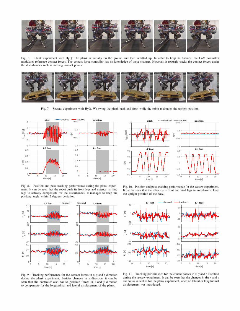
Fig. 6. Plank experiment with HyQ. The plank is initially on the ground and then is lifted up. In order to keep its balance, the CoM controllermodulates reference contact forces. The contact force controller has no knowledge of these changes. However, it robustly tracks the contact forces underthe disturbances such as moving contact points.

Fig. 7. Seesaw experiment with HyQ. We swing the plank back and forth while the robot maintains the upright position.

-2

-1

0

1

2

-C

OM

[deg

]

pitch

0.5

0.55

0.6

0.65

z [m

]

positiondesired tracked

0 5 10 15 20

time [s]

0

0.1

0.2

0.3

0.4

z [m

]

LF foot

0 5 10 15 20

time [s]

0

0.1

0.2

0.3

0.4LH foot

Fig. 8. Position and pose tracking performance during the plank experi-ment. It can be seen that the robot curls its front legs and extends its hindlegs to actively compensate for the disturbances. It manages to keep thepitching angle within 2 degrees deviation.

-50

0

50

100

Fx [N

]

LF foot

-50

0

50LH foot

-50

0

50

Fy [N

]

desired tracked

-50

0

50

0 5 10 15 20

time [s]

0

100

200

300

Fz [N

]

0 5 10 15 20

time [s]

0

200

400

Fig. 9. Tracking performance for the contact forces in x, y and z directionduring the plank experiment. Besides changes in z direction, it can beseen that the controller also has to generate forces in x and y directionto compensate for the longitudinal and lateral displacement of the plank.

-2

-1

0

1

2

-C

OM

[deg

]

pitch

0.5

0.55

0.6

0.65

z [m

]

positiondesired tracked

0 5 10 15 20

time [s]

-0.2

-0.1

0

0.1

0.2

z [m

]

LF foot

0 5 10 15 20

time [s]

-0.2

-0.1

0

0.1

0.2LH foot

Fig. 10. Position and pose tracking performance for the seesaw experiment.It can be seen that the robot curls front and hind legs in antiphase to keepthe upright position of the base.

-20

0

20

Fx [N

]

LF foot

-20

0

20

LH foot

-20

0

20

Fy [N

]

desired tracked

-20

0

20

0 5 10 15 20

time [s]

100

200

300

Fz [N

]

0 5 10 15 20

time [s]

150

200

250

300

Fig. 11. Tracking performance for the contact forces in x, y and z directionduring the seesaw experiment. It can be seen that the changes in the x and yare not as salient as for the plank experiment, since no lateral or longitudinaldisplacement was introduced.