FARM SIZE AND DETERMINANTS OF AGRICULTURAL

PRODUCTIVITY IN UKRAINE

by

Hanna Teryomenko

A thesis submitted in partial fulfillment of the requirements for the degree of

Master of Arts in Economics

National University “Kyiv-Mohyla Academy” Master’s Program in Economics

2008

Approved by ___________________________________________________ Mr. Volodymyr Sidenko (Head of the State Examination Committee)

Program Authorized to Offer Degree Master’s Program in Economics, NaUKMA

Date __________________________________________________________

National University “Kyiv-Mohyla Academy”

Abstract

FARM SIZE AND DETERMINANTS OF

AGRICULTURAL PRODUCTIVITY IN UKRAINE

by Hanna Teryomenko

Head of the State Examination Committee: Mr. Volodymyr Sidenko, Senior Economist

Institute of Economy and Forecasting, National Academy of Sciences of Ukraine

This paper tests the hypothesis of inverse relationship between farm size

and productivity for Ukrainian farmers. Several approaches were applied in

order to determine which factors, and in particular how land size effect farm

productivity. The value of output per hectare and technical efficiency were

taken as a measure of farm productivity. Technical efficiency was estimated by

two methods – non parametric DEA and parametric SFA. It was found that

the relationship between farm size and productivity is nonlinear – productivity

rises first and then falls. Ukrainian farms were found to be highly unproductive

due to inefficient use of land resources. The calculated optimum size of land

plot was determined to be larger than the average actual size of own

landholding, and this might be an important argument for canceling of land-

selling moratorium in Ukraine.

ii ii

TABLE OF CONTENTS

List of figures ………………….…………………………… iii

Acknowledgement …………….…………………………… iv

Introduction ..………………….………… ………………… 1

Literature review ……………………………….…………… 5

Methodology ……………………………………………….. 14

Data description …………....……………….………………. 24

Estimation results …………………….…..………………… 20

Conclusion ……………..………..……………….…………. 36

Bibliography ……………………………………….……….. 39

Appendix ……………………………………………….……45

iii iii

LIST OF FIGURES

Number Page Figure 3.1 DEA - estimator of Farrell input oriented technical efficiency …..…………... 19 Figure 3.2 The relationship between the farm size and its efficiency ……….……....…… 20

iv iv

ACKNOWLEDGMENTS

The author wishes to convey deepest appreciation to Iryna Lukyanenko and

Tom Coupe for their supervision and giving me valuable comments and

suggestions. I am grateful to Olesya Verchenko, Oleksandr Shepotilo, Pavlo

Prokopovych, Olena Nizalova and Hanna Vakhitova who provided thoughtful

recommendations.

I also thank Andriy Tovstopyat for his help and important advices. And

finally, I give my special thanks to Konstantin Teryomenko for his support and

encouragement.

1 1

C h a p t e r 1

INTRODUCTION

The continuous growth of world’s population, urbanization,

industrialization and global warming impose an additional burden on agriculture

enterprises. As World Bank experts predict, the demand for agriculture

products will increase twice by 2030. Therefore, countries that are major in

agriculture production should increase their productivity to satisfy future excess

demand, taking into account that less land and water resources will be available

in the future. Ukraine is one among the minority of countries which have good

conditions for the cultivation of plants (temperature, climate, dense net of

rivers and lakes and fertile land). In the Soviet Union, it was called the “bread

basket” because of the production of large amounts of wheat; however,

nowadays the role of agriculture continues to decrease.1 Therefore, it is of great

importance to investigate what are the ways of reviving and increasing the

productivity of Ukrainian agriculture and to find out which factors have

significant impact on farm productivity.

1 In 1990 51009 thousands tons of wheat were produced comparing to 34258 thousands of tons in 2006 (in a

year, that officially was announced as the year of village). Worth mentioning that areas used for cropping decreased less than by 5%. http://ukrstat.gov.ua/control/uk/localfiles/display/operativ/operativ2006/sg/sg_rik/sg_u/rosl_u.html

2 2

This paper investigates one of the most discussed and interesting

hypothesis in agriculture literature about the importance of farm scale: that the

productivity of a farm increases with the decrease of land holding’s size. The

concern about this factor of productivity arose in the mid 50ies of the last century

when the Indian Farm Management Survey found out that with the increase of

farm size the output per acre decreases. This unexpected result provoked

researchers to check whether the inevitability of this relationship is really correct.

Since that time numerous studies were done for different countries (Sen (1966)

and Carter (1984) for India, Helfand (2003) for Brazil, Swinnen (2001) for

Germany, Thapa (2007) for Nepalese mid-hills and others), however the debate

on this hypothesis is still open. That is mostly due to the fact that earlier studies

are severely criticized by some recent works (Sampath (1992), Newell et al (1997),

Rios and Shively (2005)) as more advanced methodologies and high-quality data

is available nowadays. The fact that farm size and productivity are negatively

related which before was taken for granted now has become doubtful. Such

research is of particular importance for countries which are major in agriculture

because the approval of this hypothesis may give a stimulus to land redistribution

among farmers in order to maximize country’s productivity.

Nowadays in Ukraine there are approximately 43 thousands farms and

about 600 thousands private landowners, which are the members of the

Ukrainian Association of Farmers and Landowners. According to statistics,

farmers own more than 3 millions ha of agricultural land and rent 2-2,3 millions

3 3

ha. In developed countries during the last decade the average farm size has being

increased annually on average by 1,6% ( particularly, in USA – by 1,2%, in Japan

– by 2,6%). However due to moratorium on land selling, Ukrainian farmers can’t

change the size of their own landholdings. Such ambiguous situation with land

property rights can substantially influence farms’ productivity. Since 2001 this

question remains opened because of the deputies’ opposite position on whether

to permit land selling or not. The Blue Ribbon Commission for Ukraine (2006)

suggests that the land assets should be redistributed in favour of more efficient

forms of farming.

An alternative to land buying - land renting may not be as good, because

the quality of rented land can be lower than the renter believes. Thus, for some

crops cultivation, the land has to be unused for particular time. For example, after

the sunflower cropping, soil becomes highly exhausted and land has to “rest” for

7-8 years. As usually, land tenants are not interested in renting interruption, so the

renter can face low yields of his future crop. Therefore, operation on own land

may effect farm’s productivity in different way, than in the rented one. That is

why, in this study we’ll find the impact of own and rented land size on farm’s

productivity and conclude whether land selling should be acceptable or not.

This paper considers farm’s productivity problem, which is solved applying

several approaches. As a measure of productivity we take two variables – the

value of output per hectare (following the example of many early researches (Sen

(1975), Carter (1984), Newell at al (1997)) and technical efficiency (more recent

4 4

works of Helfand (2003), Rios and Shively (2005)). Technical efficiency is firstly

determined by non parametric (econometric) approach– Stochastic Frontier

Analysis with imposing a Cobb Douglas specification on production function.

Secondly, non-parametric approach of Data Envelopment Analysis (DEA) is

applied. These two approaches are usually used together, as they are good

supplements of each other (different manner of production function specification

and as a result different nature of bias). At the second stage our measures of

productivity will be regressed on the set of explanatory variables, employing OLS,

fixed effect and RE models.

Many earlier works on this topic (Mazumdar (1965), Rao and Chotigeat

(1981), Carter (1984), etc.) had comparatively small number of observations,

which were taken from several regions of the country. For our research we use

quite representative sample, as information about particular farms

characteristics is taken from N 50-сг form (provided by Institute of Economic

Research and Policy Consulting). It consists of approximately 2,500 private

farms and covers all Ukrainian regions during 5 years: 2001-2005.

The paper will be organized in the following way: in the second chapter

the main attainments and shortcomings in the study of this hypothesis are

analyzed. Third chapter deals with methodological framework. Data description

will be provided in chapter four. In fifth chapter empirical results and policy

recommendations about the need to implement land reform will be provided

and in the chapter six conclusions will be made.

5 5

C h a p t e r 2

LITERATURE REVIEW

The hypothesis about the inverse relationship between farm size and

productivity has been tested by many researches in different countries of the

world. The debate is still of current importance because no final conclusion has

been reached so far. The largest part of the earliest research works has decided

it is a ‘proven fact’, arguing that it should be taken into account by agronomists

and farmers who are interested in increasing their productivity. However,

starting from the end of 90ies more and more researches began to reject this

hypothesis. Therefore, in this chapter I will firstly describe those works, which

find the inverse relationship, gathering them in groups that provide particular

explanations for it. Secondly, the works that reject this hypothesis will be

presented. This category of authors criticizes the first group, pointing out on

the necessity of applying other methodologies and adding new explanatory

variables.

All studies of the relationship between land holdings and productivity are

based on the basic neoclassical model. The farm productivity can be presented

as Y= F(A, L, K), where A is characteristics of land holding, L – set of labor

characteristics and K- capital used for plant cultivation. Assuming the Cobb –

Douglas production function and taking the logarithms of both sides we get the

6 6

transcendental logarithmic function, which can be estimated by different

methods and supplemented by some explanatory variables.

Mazumdar (1965) is one of the pioneers who have determined that with

the increase of land holdings of a farm, its productivity decreases. Using the

data for two districts in Uttar Pradesh (India) for 1955-1956, he also found that

returns to inputs of one acre of land is decreasing, so increasing the input the

output per unit of input decreases. Nowadays factors of production

substantially differ from those analyzed in this paper: the agriculture developed

extensively and bullock labor was one of the most important factors of the

plants production. This fact as well as limited number of farms studied were

later criticized and attracted many other researches to study this problem.

Mazumdar explained the inverse relationship between farm size and

productivity by the fact that family labor is used for cropping on small farms

and hired labor is used on large farms. It may be clarified by means of incentive

economics: the motivation for more productive work is higher for family

members rather than for hired workers. The last ones, as a rule, are used by

large farms. It may also be true, that families in small farms will use other

factors of production more intensively to produce the planned amount of

product. This explanation is also supported in works of Sen (1966), Griffin et

al. (2002), Benjamin (2002) and others.

7 7

Carter (1984) using a small household sample (376 holdings) confirmed

the inverse relationship. The data was pooled because of its poor quality, as

farmers recorded the required observations not properly. He suggested that the

inverse relationship have happened not because of sample selection bias or

‘misidentification of village effect’, but because of ‘capitalistic mode of

production’. He cites as an explanation to inverse relationship quite

controversial argument the impact of which is decided to be opposite by many

researches and will be discussed later in this chapter: ‘intra village soil quality

difference’ partly explains the negative relationship between farm size and its

productivity. He completely confides in the empirical part, pointing out that

‘overall statistical analysis strongly supports’ his beliefs.

The other main reason why the inverse relationship may occur is that a

risk-averse farmer tends to redistribute his time-labor efforts between

alternative employments. This idea is proposed by Srinivasan (1972), who have

suggested that the desire to substitute from risky activity is higher for the

landowners of larger farms, as the success of harvest is uncertain. Using the

assumption that farmer is risk-averse person of an Arrow - Pratt type (he will

become more risk averse if his wealth decreases), the author argues that among

two types of income sources, smaller farms will choose less risky self cultivation

rather than wage labor.

Two other motivations for large farms division into smaller ones are

geographic differences of studied regions and diminishing returns to scale.

8 8

However, the last one is not properly studied in empirical literature. Berry and

Clinc (1979) have pointed out, that the returns to scale are approximately

constant. Newell et al (1997) suggested that if there would be decreasing returns

to scale, the land holdings were to decrease continually to the smallest pieces of

land.

By the mid 70th approximately twenty works were devoted to study this

phenomenon in India agriculture (Sen (1975)). Almost all of them as well as

researches of Eastern Europe, Asia and Latin America agreed on negative

relationship between size of a farm and productivity (Bardhan, 1973).

The first shortcoming of the earlier works, however, was that they used

not complete micro data of FMS which was available only for limited number

of Indian districts. Deodalicar (1981) in his literature survey points to three

works that first extended the data and got another results. Thus, Rao (1967)

failed to find any inverse relationship because he used disaggregated data

sources for other Indian districts. Ruda (1968) came up with the same results in

his research of 20 villages. Rani (1971) also didn’t detect an expected effect of

size on yields for seven out of twenty five Indian villages.

The second shortcoming was proposed by Deodalicar (1981), who

extended the understanding of this problem by pointing out the importance of

technical progress. The negative relationship is preserved only in “traditional

agriculture, and it breaks down with technical progress”. The fact that small

9 9

farms are more productive is valid only when level of agriculture technology is

low. This paper makes particular contribution to the empirical literature, as it

tests the hypothesis that the inverse relationship is valid for all Indian farms and

not for separate limited number of villages (using 247 districts during the years

after the Green Revolution (1970-1971)). However, later researches have not

relied on his explanation, as the inverse relationship is still found even for the

recent farm – level data

The misleading results of the authors may also come from the fact that

farm size is relative measurement for a large and heterogeneous sample and is

expressed in absolute value (acres). However for Indian regions that have

different climate it may be the case that for the same absolute square the size

classification will be interpreted differently. Thus for arid region Rajasthan 10

acre farm can be considered as a small farm, but for irrigated West Bengal it is a

large farm (Patnaik (1972)). Thus Chadha (1978) separated Punjab into three

agro-climatic zones. He found out that in the more ‘dynamic zones’ the

negative relationship between firm size and productivity per acre does not hold.

Bhalla and Roy (1988) suggest that the inverse relationship comes from

the unobserved difference in land fertility. They argued that in developing

countries, once the exogenous land quality variable is accounted, the inverse

relationship is ‘observed to weaken, and in many cases disappear’. Therefore,

one of the most popular hypothesis being discussed in numerous research

10 10

works may be rejected just controlling for the land fertility factor (dividing it

into particular regions). Authors tend to explain fertility differences by

Malthusian approach – in more fertile area firms are as a rule smaller and as a

result more productive.

Sampath (1992) tried to prove Bhalla and Roy’s suggestion. The

advantages of his research were such: he used data for entire India (88,046

households) and the period after the green revolution (1975-1976). The author

points out that he has used the approach of Cline (1970) and Bharadwaj (1974)

– land was divided on net sown area and gross cropped area. The reason for

that is obvious – areas at some period of time may be unused, so no outcome is

produced. The author’s innovation was to use another land characteristic – type

of irrigation. However it is closely related to previous innovations - to control

for different climatic zones or just dividing farms into particular regions. Thus,

he has found out, that controlling for irrigation facilities ‘there are no

diseconomies of scale in land use’.

Newell et al (1997) also agreed with the assumption of Bhalla and Roy

and extended the previous literature both by adding missing explanatory

variable costs of cultivation and by dividing farms by the regions on 39 clusters.

The hypothesis doesn’t hold in neighboring farms, but is proved only across

different village. To control for regional differences they included the amount

of rainfalls, population density, and dummy variables of crop zones, soil types,

11 11

altitude categories. Such regional indices as literacy rates, road and railway

infrastructure and district electrification are found to be insignificant.

However, shortcomings of the previous works are not only the data

specifications and its quality, but also the methodology used. In recent works

(Townsend (1998), Mathijs, Swinnen (2001), Helfand (2003) and others) to

measure the productivity efficiency the Data Envelopment Analysis (DEA) is

used, which was firstly suggested by Farrell (1957). This nonparametric

approach allows to measure technical and allocation efficiencies without

imposing any functional form on the production function. As it doesn’t allow

testing direct hypothesis, two steps should be used: to get the inefficiency

measures using DEA and then regress it on the set of explanatory (farm

specific characteristics). This methodology will be presented in details in the

third chapter of this research work.

Townsend et al (1998) claims that he is among the first researchers, who

used this new methodological approach (of DEA) and ‘recent farm survey

data’. The research was conducted for wine producing farms in South Africa.

The farm productivity was estimated both as separated partial and total

productivity. The author has found out that the inverse relationship is weak and

total factor productivity deviates from region to region. Therefore, his empirical

research has contributed to the agronomists’ world discussion the conclusion

that hypothesis of inverse relationship may be invalid.

12 12

Helfand (2003) have shown that the relationship between farm size and

productivity is more complex than it was earlier believed. Applying Data

Envelopment Analysis (DEA), the U-shaped relationship was determined: the

productivity first falls (for farms up to 200 hectares) and then rises. He avoided

the aggregation bias by using the data from 426 counties, 4 types of land tenure

and 15 classes of farm size. However, as he didn’t have access to farm level

data, the representative farm was introduced for each type of farm

characteristics, as a result 237,595 observations were aggregated into 9,304. He

followed the approach proposed by Vicente et al (2001), who proposed to

measure total factor productivity (TFP) which accounts land, labor and inputs

productivity. Worth mentioning, all previous works determined the impact of

farm size on land (of one acre) and labor productivity.

For the first stage of DEA estimation Helfand (2003) used several

methodologies: to account for spacial heterogeneity - fixed effect, for

heteroscedasticity across 426 counties - RE and for spacial correlation in the

errors across counties - SUR framework. As explanatory variables of technical

efficiency he used 6 types of farm characteristics: farm size, land tenure (type of

ownership), composition of cattle, access to institutions and use of public

goods, technology and inputs. All of them had statistically significant impact on

farm efficiency, however, only high farm specialization, access to institutions (to

credit, electricity and technical assistance) and the level of technology had large

influence. The author argues that if small farms had at least the same access to

13 13

institutions, technology and inputs, as large farms did, their efficiency will be

higher (than of the last ones).

Rios and Shively (2005) studied the impact of farm size on productivity

using the data on coffee farms in two districts of Vietnam. Using the two steps

analysis (DEA and Tobit regression) he also disproved the hypothesis of

inverse relationship and identified which factors of production influence

technical and cost inefficiency (long pipe lines, farmer’s level of education).

One of the main factors that affect large farms to be more efficient is that they

have access to credit and investment.

Therefore, no increasing return to size of small farms was proved both in

developing and developed countries by many researches in 70-90th. However,

recent works have shown that the larger the land holding – the larger is farm

productivity. This conclusion is made for countries with developed agriculture,

where the farms are equipped with modern technology and have a free access

to credit. It is important to define what is the best land policy for Ukrainian

farms at this transition period. Thus, if productivity of farm increases with land

holding, a good policy will be the abolition of moratorium. We should also take

into account not typical to other countries high ability of Ukrainian farmers to

rent land. If productivity will increase with total land, but decrease with

increasing the size of rented lend, it will be another argument for allowing

selling of the land.

14 14

C h a p t e r 3

METHODOLOGY

In order to estimate farm’s productivity several approaches will be used in

this paper. Firstly, we’ll consider a parametric (econometric) approach of

estimation the farm productive efficiency (Stochastic Frontier Analysis), secondly

we’ll use non-parametric (operational) approach - Data Envelopment Analysis

(DEA), which will help to find out what are the main determinants of Ukrainian

farms efficiency and what the impact of size is. And thirdly we will use an

alternative measure of farm’s efficiency – value of output per hectare. The

combination of two efficiency estimation methods is used in many recent works

for different countries, where the hypothesis of inverse relationship between farm

size and productivity was tested: Zyl, Miller, Parker (1996) for Poland, Mathijs

and Swinnen (2001) for East German agriculture, Helfand (2003) for Brazil,

Masterson (2007) for Paraguay agriculture and others.

It is a good tradition to use DEA and SFA techniques together because

each of them has its advantages and disadvantages (Felthoven (2000)). They differ

in the manner of production frontier generation; as a consequence, the source of

the result’s bias is different. For the SFA estimation we need to assume a specific

form of production function (usually a Cobb-Douglass), therefore actual results

can be biased due to incorrect specification. The strong point of SFA is that it is

15 15

robust to random noise. DEA is used as alternative to SFA when it is difficult to

specify the correct SFA model. It constructs a piecewise linear representation of

the technology frontier using mathematical programming. A weak point of non-

stochastic DEA approach is that it is sensitive to random noise. Such different

approaches to production frontier construction can sometimes yield different

results and the researcher has to choose analytically which results are more

appropriate to the theoretical model.

Efficiency in parametric approach (also called a regression technique) is

calculated by comparing the observed output with the optimal (maximum) output

for the same input. We describe below a Cobb-Douglas specification of

production function, as it is commonly used for stochastic production function

estimation.

Consider a farm that operates using a set of inputs: capital K, family and

hired labor L and A acres of land (which consists of own and rented land) for

producing output Y.

To construct SFA estimation we have to assume that the actual output of

a particular farm i at time t is a function F(·) of the set of inputs and error term εit,

which consists of two parts: TEit – technical efficiency and eit – statistical noise,

which is purely random variation in output. Assume that these two components

of error term enter the function multiplicatively.

Yit=F(Ait, Kit, Lit) ·TEit·eit (1)

16 16

Taking the logarithm of both sides and denoting yit = log(Yit), f= log (F),

uit=-log (TEit), vit=log(eit) , we get

Yit=f(Ait, Kit, Lit)-uit+vit

(2)

To find technical efficiency term u we have to impose functional form on

f(·) and to assume the distribution of statistical noise v and efficiency term u. Let’s

assume Cobb-Douglas production function to estimate the production function

frontier

F(Ait,Kit,Lit)=AitαKit

βLitγ (3)

Taking the logarithm of equation (3), the resulting production function

frontier specification with u≥0 can be presented in the form:

lnyit= α0 + α1ln At + β1 ln K1t+ β2 ln K2t+…+ βk ln Kkt + γ1ln L1t + γ2ln

L2t + …+γkln Lkt + η1T01+ η2T02+ η3T03+ η4T04+ η5T05 -uit+vit, (4)

where α0 is an intercept, yit is the total annual farm output per hectare (deflated by

CPI) , A - the size of a farm, Ti- dummy variable for time, α1, βk, γk are

production elasticities for input k.

We assume that uit is half-normally distributed with mean µ and variance

σv2 and vit is normally distributed with zero mean and variance σu

2.

Estimation of this model will give us the possibility to compare actual and

predicted output for each farm, thus to determine its technical inefficiency. We’ll

do this firstly, by setting uit=0, so if there is technical inefficiency (uit≠0), the level

17 17

of output is below the frontier (Kumbhaker and Lovell (2000)). Secondly, for

panel data we will use time-varying decay model (Battese and Coelli (1992)).

Technical efficiency is redefined as

uit= ηiui= ui exp(-η(t-Ti)) (5)

Where η is decay parameter, Ti – the last time period in the i panel. When

η=0 the degree of inefficiency is constant over time (time invariant model), η>0

inefficiency decreases with time, η<0 – inefficiency increases.

Obtained scores of technical efficiency we regress on farm characteristics,

farm management set, input set and regional dummies. We will use OLS, fixed

effect and random effect approaches and define the effect of farm size on

productivity. As farm characteristics we use the amount of own and rented land,

as farm management characteristics2 - technical and marketing assistance.

Secondly, let’s estimate the farm productive efficiency using the non

parametric approach (DEA). As mentioned above we don’t need to impose a

functional form on production function, because nonparametric deterministic

frontier is determined using linear programming approach. That is, the distance

between efficiency frontier and observed input-output combinations gives the

value of technical inefficiency.

Total technical efficiency (TTE) can be decomposed into two

components: scale efficiency (SE) and pure technical efficiency (PTE) (Mathijs,

2 Marketing costs and expenditures on leased equipment (Masterson (2007)). However, it is a relative division,

as expenditures on leased equipment can also be referred to input set.

18 18

Swinnen (2001)). Mathematically, total technical efficiency under CRS can be

presented in terms of minimizing inputs per unit of outputs

TTE (yj, xj)=min θ

s.t. Σzk ykm ≥ym

j , m=1,…,M

Σzk xik ≤θxi

j i=1,…,N

θ≥0, zk≥0

where θ is the ratio of observed to the maximum (efficient) vector of inputs, yjm is

the output of activity m of farm j, xij – the vector of inputs, z – intensity of each

activity (the arbitrary positive scalar which reflects radial expansion / contraction

of observation k).

Thus, assuming that proportionate expansion or contraction of vectors of

inputs and outputs will remain in the technology set T, and that intensity z of

each farm is non negative, the linear programming model finds the minimum

value of θ.

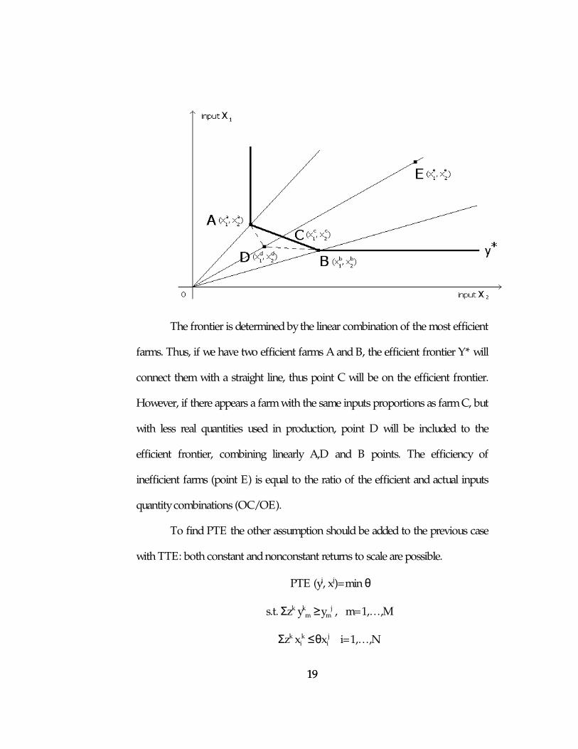
Graphically the DEA - estimator of Farrell input oriented technical

efficiency can be presented as a locus of the efficient points3:

3 For simplicity, we depict two-input case.

19 19

The frontier is determined by the linear combination of the most efficient

farms. Thus, if we have two efficient farms A and B, the efficient frontier Y* will

connect them with a straight line, thus point C will be on the efficient frontier.

However, if there appears a farm with the same inputs proportions as farm C, but

with less real quantities used in production, point D will be included to the

efficient frontier, combining linearly A,D and B points. The efficiency of

inefficient farms (point E) is equal to the ratio of the efficient and actual inputs

quantity combinations (OC/OE).

To find PTE the other assumption should be added to the previous case

with TTE: both constant and nonconstant returns to scale are possible.

PTE (yj, xj)=min θ

s.t. Σzk ykm ≥ym

j , m=1,…,M

Σzk xik ≤θxi

j i=1,…,N

20 20

θ≥0, zk≥0

Σzk =1

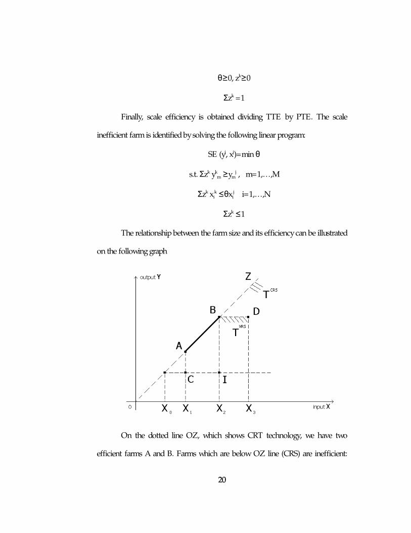
Finally, scale efficiency is obtained dividing TTE by PTE. The scale

inefficient farm is identified by solving the following linear program:

SE (yj, xj)=min θ

s.t. Σzk ykm ≥ym

j , m=1,…,M

Σzk xik ≤θxi

j i=1,…,N

Σzk ≤1

The relationship between the farm size and its efficiency can be illustrated

on the following graph

On the dotted line OZ, which shows CRT technology, we have two

efficient farms A and B. Farms which are below OZ line (CRS) are inefficient:

21 21

farms C and D. Points A, B, C, D become technically efficient (form the efficient

frontier) when non constant returns to scale is assumed. Scale efficiency is

received after the extracting pure technical efficiency from total technical

efficiency. Thus, small farm C and large farm D are technically efficient, but are

not scale efficient. The value of scale inefficiency for the farm C is OX0/OX1,

and for D is OX2/OX3. Farm, such as I are both technically (by OX1/OX2 ) and

scale inefficient (OX0/OX1), so the total level of inefficiency is equal to

OX0/OX2.

It is important to note that the term “inefficiency” is used to denote the

distance between the actual output and the efficient frontier. “Inefficient” farm

behavior can be explained by a lot of other reasons that are not related to X-

inefficiency: market failures, quality of rented land, credit market constraint and

others. For our second stage we regress obtained technical efficiency scores as

well as output per hectare (using pooled OLS, fixed effect and random effect

approaches) on farm size, land tenure (the impact of own and rented

landholdings), composition of output (wheat, corn, sunflower, barley and

horticultures), access to institutions/ public goods (electricity, technical assistance,

leased equipment and property), inputs (labor, machines, fertilizer, fuel spent) to

determine how they effect technical efficiency.

Pooled OLS can be not a good approach to find the impact of different

factors on farm productivity as it does not account for the unobserved

characteristics of the farms. As a result we will have omitted variables bias. To

22 22

coupe with this problem we will use fixed effect and random effect approaches.

Fixed effect will be used in order to get rid of the variation in farms constant with

time, however if there is no correlation between unobserved fixed characteristics

and explicative variables – we will use random effect.

There can arise several problems which are related to the second stage

estimation. We will briefly discuss those, which are more likely to happen. First of

all, there can be a problem of multicollinearity, because as we have panel data, in

all variables there can be presented the same trend, e. g. farmers with larger land

holdings use more humus and fertiliser than those with smaller ones. If

dependent variables are highly collinear, OLS estimators will have larger variance

and covariance and as a result estimates will be not precise. To account for

correlations in standard error of each farm over time we will use clustering by

farms.

Secondly, there can be a problem of heteroscedasticity which may happen

due to several reasons: presence of outliers, incorrect specification of regression

model and the so called “error-learning model”, which means that farmers get

experience in cropping with time, and their behavior errors become smaller.

Though heteroscedasicity does not bias the coefficients, it biases the standard

errors, and this may lead to the incorrect specification of our results. We will use

Breush - Pagan test to detect its presence and estimate robust standard errors

(Huber/White estimators) to deal with it.

23 23

Finally, we want to draw attention to another possible problem -

endogeneity of productivity. This may happen because not the land holdings

influence the farm productivity, but the past farmer’s experience influences his

choice to choose the proper land holdings in order to maximize productivity. If

we have this problem, estimated results will be biased. To test the validity of the

assumption of no endogeneity Durbin-Wu-Hausman test will be used. In case of

endogeneity we should use instrumental variables, however as we haven’t found

no appropriate ones used in the literature, and because we have micro-level data

with limited number of explanatory variables, we can only use lags of land

holdings.

As Ukrainian farmers operate on the land market only by renting the

land, this may influence their efficiency. The reason for that may be due to

imperfect knowledge of the quality of rented land, which can be lower than they

believe (e.g. due to uninterrupted use) and they have less motive to invest in land.

Akerlof (1970) shows that market with imperfect information (when sellers are

better informed than buyers) can shrink or even disappear. Therefore, it is

important to determine both how the total land holding and the use of rented

land influences the farm productivity.

24 24

C h a p t e r 4

DATA DESCRIPTION

The empirical analysis is based on the balanced data sample of 1170

Ukrainian private farms during the 2001-2005 years. Because of not full and

proper initial data set, in which we had some missing farms for some years, we

had to deleted them in order to create balanced data sample (which is needed for

DEA and SFA approaches).

We have compared results, obtained by the parametric approach for

balanced and unbalanced panel data (see Table A.5) and concluded that there is

no difference if we drop some observations. The particular farm characteristics

are taken from N 50-сг form, which was collected by State Committee of

Statistics (Derzhkomstat) and provided by the Institute for Economic Research

and Policy consulting (IER). To control for specific climate conditions and

original land fertility the territory of Ukraine the regional dummy variable was

used.

The data set allows using for the empirical analysis such information (the

descriptive statistics is presented in the table below):

25 25

- For every specific crop: production (in metric centners), the cost of

production (thd. UAH), number of workers, the cost of sold products, sales

revenue (thd. UAH).4

- Costs of: labor (wage bill), mineral fertilizers, fuel, electricity, repairs,

depreciation, payments for rented land, payments for rented property, the use of

an input for production, total (thd UAH), the use of an input in crop production

-Farms’ financial results: from selling agricultural products: profit( thd

UAH), loss (thd UAH), other revenue (thd. UAH), other losses (thd. UAH), net

profits (thd. UAH), net loss (thd. UAH), farm profitability, average annual value

of fixed and variable (floating) assets (thd. UAH), average annual number of

workers employed in production, administrative costs, marketing costs.

- Land use: total, leased, agricultural land, total including arable land,

hayfield, pastures.

Data set also allows us to control for farm specialization in a particular

year. Therefore, dummy variables for crop, grain, sunflower, sugar-beet, animal

and multi crop specialization will be included into the regression.

We should control for these factors as they may have an important effect

on the farms productivity.

According to our statistics Ukrainian farmer on average has 45,7 hectares

of own land and can rent up to 5000 hectares (some large farmers, with a large

4 All the monetary values are corrected for CPI with 2001 as a base year.

26 26

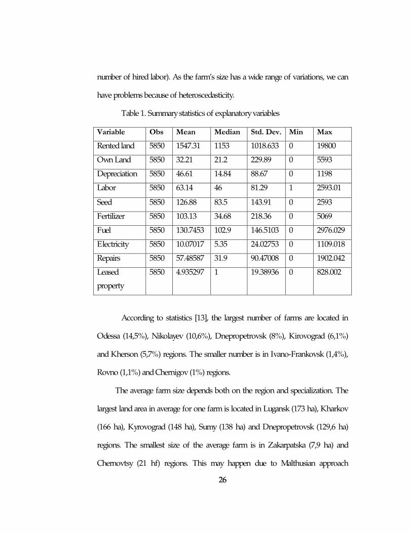
number of hired labor). As the farm’s size has a wide range of variations, we can

have problems because of heteroscedasticity.

Table 1. Summary statistics of explanatory variables

Variable Obs Mean Median Std. Dev. Min Max

Rented land 5850 1547.31 1153 1018.633 0 19800

Own Land 5850 32.21 21.2 229.89 0 5593

Depreciation 5850 46.61 14.84 88.67 0 1198

Labor 5850 63.14 46 81.29 1 2593.01

Seed 5850 126.88 83.5 143.91 0 2593

Fertilizer 5850 103.13 34.68 218.36 0 5069

Fuel 5850 130.7453 102.9 146.5103 0 2976.029

Electricity 5850 10.07017 5.35 24.02753 0 1109.018

Repairs 5850 57.48587 31.9 90.47008 0 1902.042

Leased

property

5850 4.935297 1 19.38936 0 828.002

According to statistics [13], the largest number of farms are located in

Odessa (14,5%), Nikolayev (10,6%), Dnepropetrovsk (8%), Kirovograd (6,1%)

and Kherson (5,7%) regions. The smaller number is in Ivano-Frankovsk (1,4%),

Rovno (1,1%) and Chernigov (1%) regions.

The average farm size depends both on the region and specialization. The

largest land area in average for one farm is located in Lugansk (173 ha), Kharkov

(166 ha), Kyrovograd (148 ha), Sumy (138 ha) and Dnepropetrovsk (129,6 ha)

regions. The smallest size of the average farm is in Zakarpatska (7,9 ha) and

Chernovtsy (21 hf) regions. This may happen due to Malthusian approach

27 27

(difference in climate and land fertility) and the farm specialization. 5 Our

statistics differs from the official statistics, because our sample includes only

limited number of observations (as mentioned above, there are 43 thousands

farmers in Ukraine, but we have about 2500). Unfortunately, the smallest farms

don’t have to submit any statistical reports; therefore we can have a problem with

sample selection bias. However, As Ukrainian farmers can’t buy land, but only

rent it, we are particularly interested in those farmers that can afford to rent land

and to hire labor to work on that land. To determine the impact of the rented

land size on it’s productivity, we have to use data of those farmers that rent land.

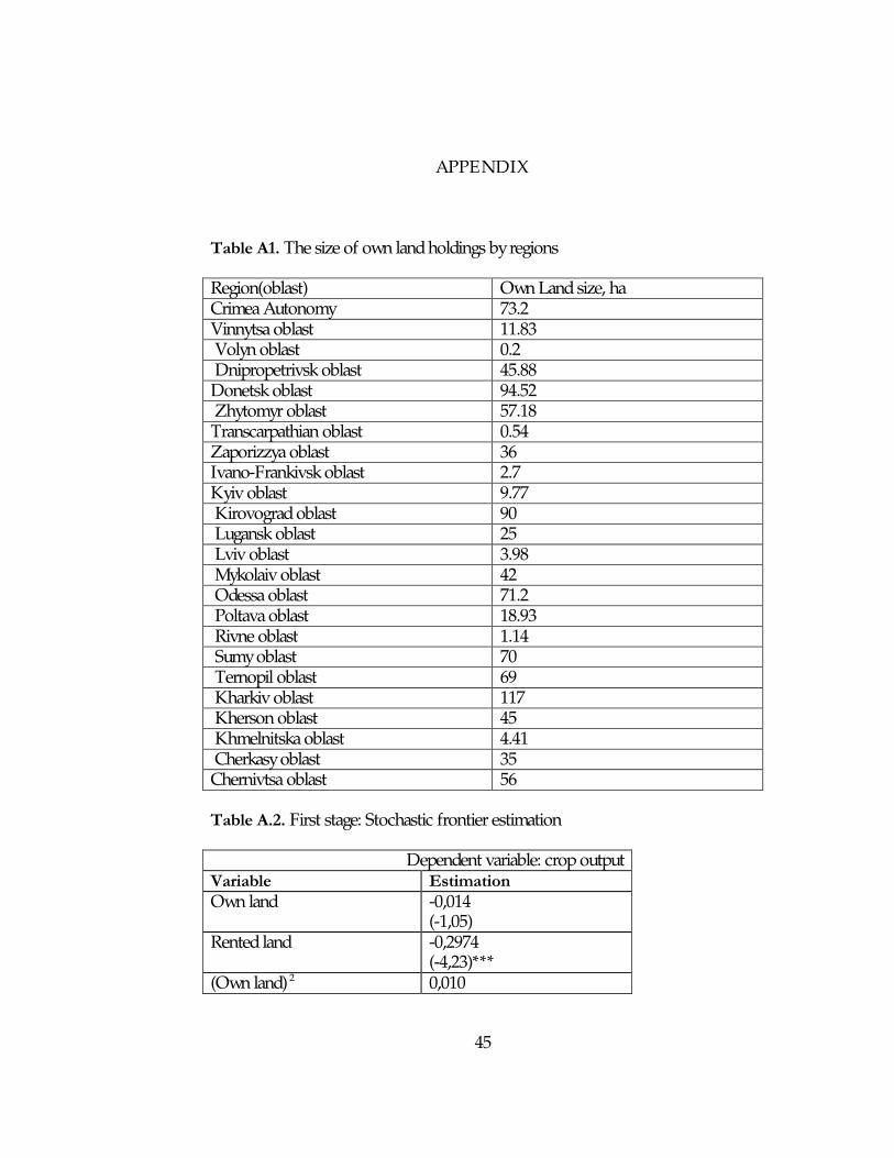
As can be seen from the TableA.1, we have a quite representative sample,

as the size of own land holdings are comparatively similar to the official statistics.

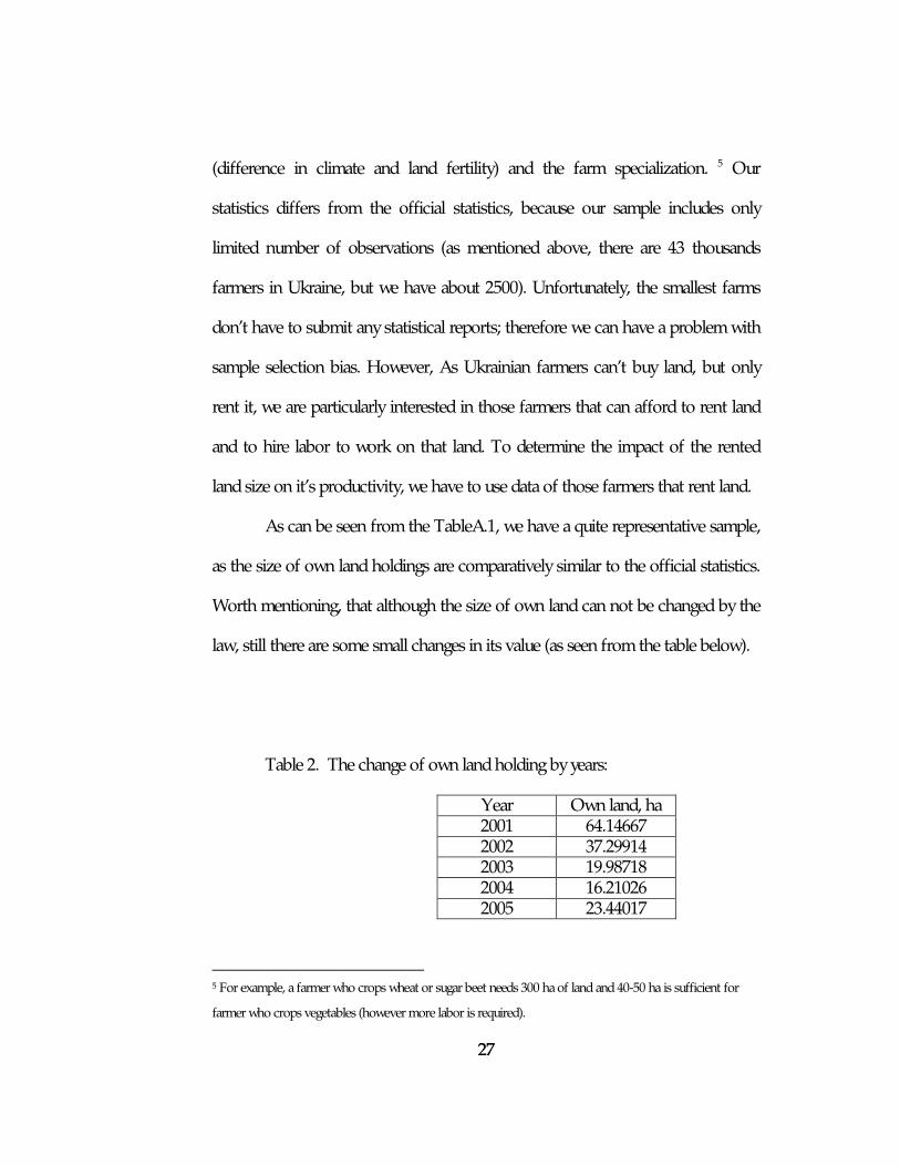
Worth mentioning, that although the size of own land can not be changed by the

law, still there are some small changes in its value (as seen from the table below).

Table 2. The change of own land holding by years:

5 For example, a farmer who crops wheat or sugar beet needs 300 ha of land and 40-50 ha is sufficient for

farmer who crops vegetables (however more labor is required).

Year Own land, ha 2001 64.14667 2002 37.29914 2003 19.98718 2004 16.21026 2005 23.44017

28 28

As some analysts mention there are some possibilities to overcome low –

and the land can “move” between land owner and middlemen. The descriptive

statistics by the year shows that the maximum land holdings were in 2001, than

they decreased by 2004 and in 2005 they again started to grow.

29 29

C h a p t e r 5

ESTIMATION RESULTS

We will start discussion of our results from presenting the values of

technical efficiencies, obtained first, by SFA approach, and second, by DEA

method. Then, more important for testing our hypotheses results will be

presented: which factors effect farm productivity. As mentioned above, for this

second stage we’ll use three dependent variables: value of output per hectare

and technical efficiencies, estimated in the first stage by two approaches.

For obtaining the scores of technical efficiency by SFA approach we used

Stata 10 and by DEA method - program DEAP; for our second stage

estimations we applied Stata 9. Worth mentioning that for DEA estimation

other software can be used, in particular Matlab.

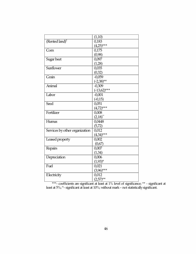
Since we are interested in the estimates of technical efficiency and not in

the frontier per se, we will present the results of the first stage estimation of

stochastic frontier in the Appendix (Table A.2) and skip the discussion of the

coefficients. Worth mentioning, that the majority of coefficients are statistically

significant at least at 1% level of significance (due to individual t-tests).

To estimate technical efficiency by DEA approach we used 1-output-4

inputs model (total crop production as unknown function of labor, land size,

purchased inputs and technical expenses). Inputs were assumed to be free

30 30

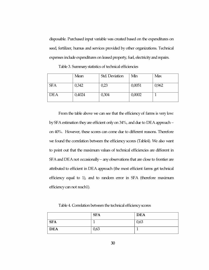
disposable. Purchased input variable was created based on the expenditures on

seed, fertilizer, humus and services provided by other organizations. Technical

expenses include expenditures on leased property, fuel, electricity and repairs.

Table 3. Summary statistics of technical efficiencies

Mean Std. Deviation Min Max

SFA 0,342 0,23 0,0051 0,962

DEA 0,4024 0,304 0,0002 1

From the table above we can see that the efficiency of farms is very low:

by SFA estimation they are efficient only on 34%, and due to DEA approach –

on 40%. However, these scores can come due to different reasons. Therefore

we found the correlation between the efficiency scores (Table4). We also want

to point out that the maximum values of technical efficiencies are different in

SFA and DEA not occasionally – any observations that are close to frontier are

attributed to efficient in DEA approach (the most efficient farms get technical

efficiency equal to 1), and to random error in SFA (therefore maximum

efficiency can not reach1).

Table 4. Correlation between the technical efficiency scores

SFA DEA

SFA 1 0,63

DEA 0,63 1

31 31

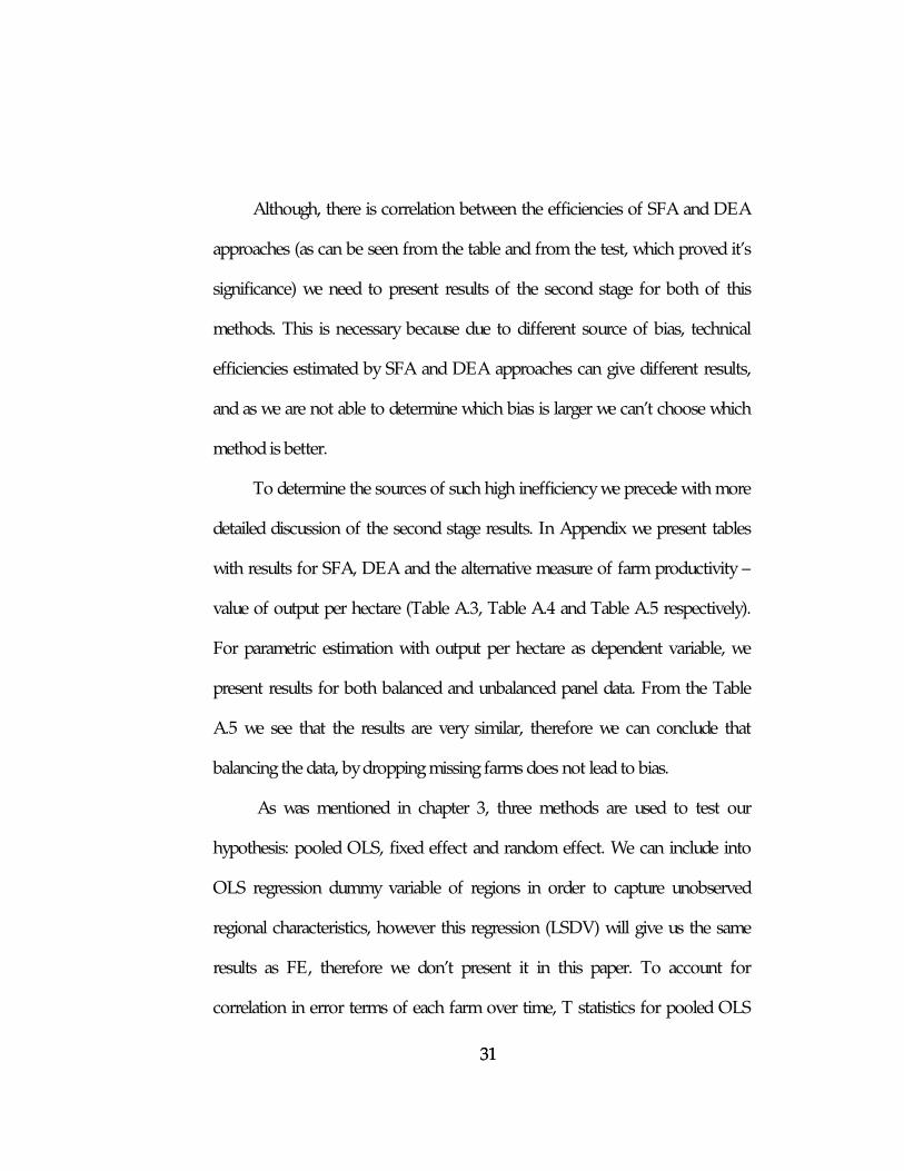
Although, there is correlation between the efficiencies of SFA and DEA

approaches (as can be seen from the table and from the test, which proved it’s

significance) we need to present results of the second stage for both of this

methods. This is necessary because due to different source of bias, technical

efficiencies estimated by SFA and DEA approaches can give different results,

and as we are not able to determine which bias is larger we can’t choose which

method is better.

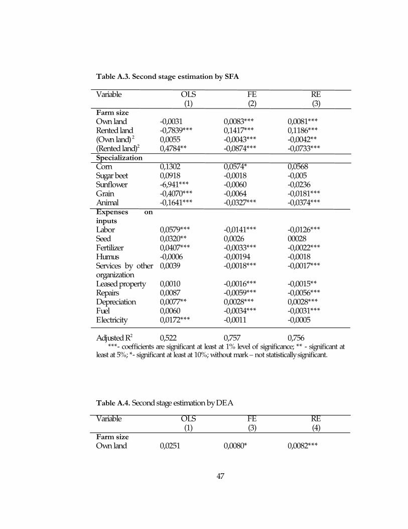
To determine the sources of such high inefficiency we precede with more

detailed discussion of the second stage results. In Appendix we present tables

with results for SFA, DEA and the alternative measure of farm productivity –

value of output per hectare (Table A.3, Table A.4 and Table A.5 respectively).

For parametric estimation with output per hectare as dependent variable, we

present results for both balanced and unbalanced panel data. From the Table

A.5 we see that the results are very similar, therefore we can conclude that

balancing the data, by dropping missing farms does not lead to bias.

As was mentioned in chapter 3, three methods are used to test our

hypothesis: pooled OLS, fixed effect and random effect. We can include into

OLS regression dummy variable of regions in order to capture unobserved

regional characteristics, however this regression (LSDV) will give us the same

results as FE, therefore we don’t present it in this paper. To account for

correlation in error terms of each farm over time, T statistics for pooled OLS

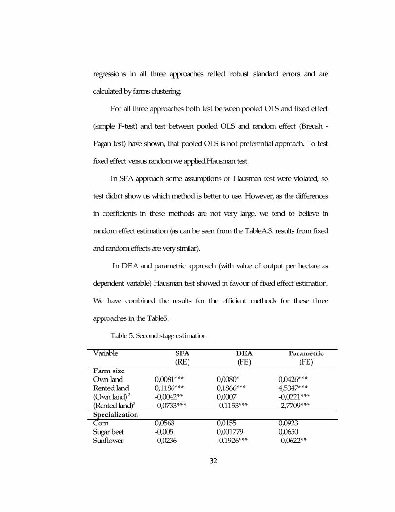
32 32

regressions in all three approaches reflect robust standard errors and are

calculated by farms clustering.

For all three approaches both test between pooled OLS and fixed effect

(simple F-test) and test between pooled OLS and random effect (Breush -

Pagan test) have shown, that pooled OLS is not preferential approach. To test

fixed effect versus random we applied Hausman test.

In SFA approach some assumptions of Hausman test were violated, so

test didn’t show us which method is better to use. However, as the differences

in coefficients in these methods are not very large, we tend to believe in

random effect estimation (as can be seen from the TableA.3. results from fixed

and random effects are very similar).

In DEA and parametric approach (with value of output per hectare as

dependent variable) Hausman test showed in favour of fixed effect estimation.

We have combined the results for the efficient methods for these three

approaches in the Table5.

Table 5. Second stage estimation

SFA DEA Parametric Variable (RE) (FE) (FE)

Farm size Own land 0,0081*** 0,0080* 0,0426*** Rented land 0,1186*** 0,1866*** 4,5347*** (Own land) 2 -0,0042** 0,0007 -0,0221*** (Rented land)2 -0,0733*** -0,1153*** -2,7709*** Specialization Corn 0,0568 0,0155 0,0923 Sugar beet -0,005 0,001779 0,0650 Sunflower -0,0236 -0,1926*** -0,0622**

33 33

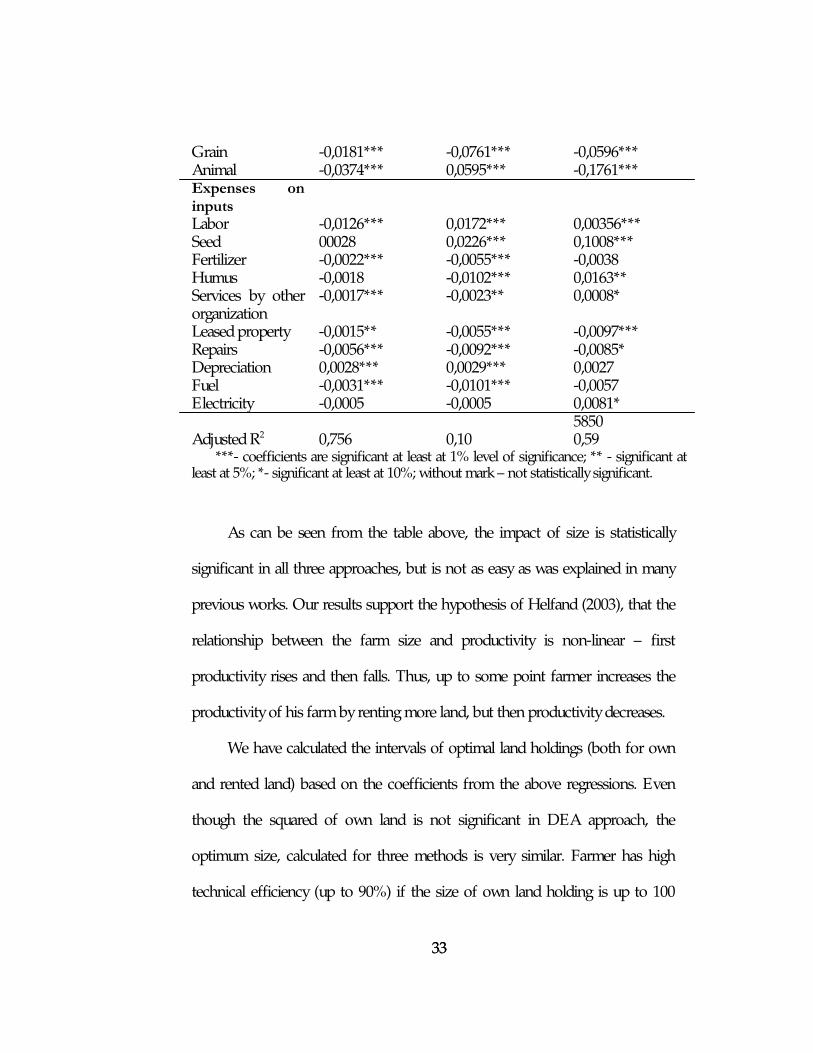
Grain -0,0181*** -0,0761*** -0,0596*** Animal -0,0374*** 0,0595*** -0,1761*** Expenses on inputs

Labor -0,0126*** 0,0172*** 0,00356*** Seed 00028 0,0226*** 0,1008*** Fertilizer -0,0022*** -0,0055*** -0,0038 Humus -0,0018 -0,0102*** 0,0163** Services by other organization

-0,0017*** -0,0023** 0,0008*

Leased property -0,0015** -0,0055*** -0,0097*** Repairs -0,0056*** -0,0092*** -0,0085* Depreciation 0,0028*** 0,0029*** 0,0027 Fuel -0,0031*** -0,0101*** -0,0057 Electricity -0,0005 -0,0005 0,0081* 5850 Adjusted R2 0,756 0,10 0,59

***- coefficients are significant at least at 1% level of significance; ** - significant at least at 5%; *- significant at least at 10%; without mark – not statistically significant.

As can be seen from the table above, the impact of size is statistically

significant in all three approaches, but is not as easy as was explained in many

previous works. Our results support the hypothesis of Helfand (2003), that the

relationship between the farm size and productivity is non-linear – first

productivity rises and then falls. Thus, up to some point farmer increases the

productivity of his farm by renting more land, but then productivity decreases.

We have calculated the intervals of optimal land holdings (both for own

and rented land) based on the coefficients from the above regressions. Even

though the squared of own land is not significant in DEA approach, the

optimum size, calculated for three methods is very similar. Farmer has high

technical efficiency (up to 90%) if the size of own land holding is up to 100

34 34

hectares. However, the optimum size of rented land should not exceed 20

hectares, as technical efficiency is very sensitive to changes in rented land.

High sensitivity to rented land change may come due to different reasons

of land inefficient use. On the one hand, farmer can rent land of lower quality

than expected (e.g. because it is exhausted by previous cropping of sunflower).

On the other, he can rent more land than is optimal to profit maximization

because of spurious expectations about the land policy6.

Next, we proceed the discussion of our results with interpreting the

coefficients of other explanatory variables. First of all, we want to point out that

labor elasticity is statistically significant in all three approaches. We draw attention

to this result, because in many research works on the micro-level data (Battese

and Coelli (1992), Felthoven (2000), Alvarez and Arias (2004)) authors found that

the impact of labor on farm productivity is not significant. From our estimation,

we can see that an increase in labor on 1% causes productivity to increase on

1,7% (according to DEA approach), on 0,3% (according to parametric approach

with output per hectare as a dependant variable) and to decrease on 1,2%

according to SFA approach. The magnitude and the sign of labor elasticity are

different in all three methods, because as was mentioned in chapter 3 all

approaches may give different source of bias.

6 Politicians in 2004-2005 suggested, that land which is rented by farmers, can be bought by them in the

future by oversimplified procedures. Later this suggestion was canceled.

35 35

The specialization of farmers can also influence productivity. Thus, we have

found out that the specialization in grain, sunflower and animal production has

negative impact on farm’s productivity. It’s a typical situation for Ukraine (and for

the majority of other countries) that farms specialized in animal production are

inefficient. Therefore, government provides special benefits for these producers

in order to stimulate production. The negative impact of specialization in grain

and sunflower can be explained by the fact, that these cultures are very

“fastidious”, sensitive to weather changes and require a lot of farmer’s efforts and

knowledge.

Many other explanatory variables have quite evident influence on

productivity. Thus, expenses on repairs negatively affect farm productivity, seed,

electricity, humus and leased property – positive (however the signs of these

explanatory variables sometimes differ depending on the method of estimation).

Summing up the results, we can conclude that there are large

inefficiencies in agriculture production of Ukraine. On average farms have 66%

(according to SFA) and 60% (to DEA) margin of actions to improve their

productivity either by increasing the efficiency of factors used or by adjusting size

of land. All specifications, used in this paper, have shown that the size of a farm

has significant impact on farm productivity, and the relationship is not linear. The

impact of other factors in general is also very similar, but sometimes their can be

some differences, which can be explained by different source of bias.

36 36

CONCLUSION

The goal of our research work was to test the relationship between farm

size and its productivity in order to provide arguments whether the moratorium

on land selling in Ukraine should be canceled or not. Using the data for 1170

Ukrainian farms during the 5 years (2001-2005) we applied several approaches

to determine which factors, and in particular how land size affect farm

productivity. As a measure of farm productivity, we took the value of output

per hectare and technical efficiency. The last one was estimated by two

methods – non parametric DEA and parametric SFA approaches.

We found out that the relationship between farm size and productivity is

non-linear. This means that up to some point productivity increases (for farms

with total land size up to 120 ha) and then decreases. We have estimated that

elasticity of rented land is higher than of own land. This means that if the

amount of land used for cropping exceeds optimum amount, productivity

decreases in a greater extent if more rented land is used.

According to our estimations, optimum size of own land is 100 hectares,

which exceeds the average own holdings of Ukrainian farmers. However, the

amount of optimum rented land (20 hectares) is significantly lower than the

actual average size of rented plots. There can be different reasons to this “over-

renting” effect. We suggest that farmers rent large plots of land, and thus

37 37

deliberately reduce their productivity (and agricultural productivity of the

country as a whole) because of political spurious promises. One of them –

farmer has ability to buy all the land, which he currently rents.

Therefore, the main argument for moratorium cancelling is the fact, that

average size of own land holding is less than the optimum for efficient

production. Renting of needed land is not a good alternative, as productivity of

this land is lower (rented land may be of lower quality (exhausted by previous

cultivation) and farmer has less incentive to invest in this land).

However, we should take into account the possibility that farmers may

want to increase their holdings of rented land in order to purchase this land in

the future (to get additional profit by reselling it). Therefore, several restrictions

should be made in the land law before the moratorium will be canceled. Thus,

one way of improving the situation on the Ukrainian land market, can be

providing a restriction on buying large sizes of land (more than 120 hectares) or

establishing a particular range for each farmer on which he can change his land

plot. This is a policy implication for the first stage – coming from moratorium –

to free market. In order to achieve maximum efficiency in agriculture

production, the access to land market should not be restricted by government.

In addition we want to present other typical fact for Ukrainian economy -

in spite of moratorium on land selling, holdings of own land of some farmers

changed from year to year. As experts comment, there are different ways to

overcome Ukrainian low, so those who have such possibility can buy / sell land

38 38

in small amounts. Therefore such restrictions are not only the sources of

inefficiency, but additional corruption. This may be another argument for

moratorium canceling.

39 39

BIBLIOGRAPHY

1. Akerlof (1970). The market for

“Lemos”: Quality Uncertainty and the

Market Mechanism/ The Quarterly

Journal of Economics, Vol. 84, # 3,

pp. 488-500.

2. Alvarez A., Arias C., 2004.

Technical efficiency and farm size: a

conditional analysis. Agricultural

Economics 241, pp 241-250.

3. Battese, Coelli (1992). Frontier

production function, technical

efficiency and panel data: With

application to paddy farmers in India.

Journal of productivity analysis.

3:153-69.

4. Bardhan, P., K., (1973). Size

Productivity, and Returns to Scale: An

Analysis of Farm- Level Data in

Indian Agriculture. The Journal of

Political Economy, Vol. 81, No. 6,

pp. 1370-1386.

5. Benjamin, D., and Brand, L.,

(2002). Property Rights, Labor

Markets, and Efficiency in a

Transition Economy: The Case of

Rural China. The Canadian Journal of

Economics, Vol. 35, No. 4, pp. 689-

716.

6. Berry, A., W., Cline (1979).

Agrarian Structure and Productivity in

Developing Countries. Baltimore,

Johns Hopkins University Press.

7. Bhalla, S., S., and Roy, P., (1988).

Mis-Specification in Farm

Productivity Analysis: The Role of

Land Quality. Oxford Economic

Papers, New Series, Vol. 40, No.1.

pp. 55-73.

8. Carter M. (1984) Identification of

the inverse relationship between farm

Size and productivity: an empirical

analysis of peasant agricultural

production. Oxford Economic paper,

New series, Vol. 36, No.1, pp. 131-

145.

9. Chadha GK (1978). Farm Size and

Productivity Revisited: Some Notes

from Recent Experience of Punjab -

Economic and Political Weekly.

10. Deolalikar A. B. (1981) “The

Inverse Relationship between

Productivity and Farm Size: A Test

43 43

Using Regional Data from India”

American Journal of Agricultural

Economics, Vol. 63, No. 2, pp. 275-

279. doi:10.2307/123956534.

11. Farrell M. J., (1957). The

measurment of productive efficiency,

Journal of the Royal Statistical Society

Series A, 120: 253-81.

12. Felthoven (2000). Measuring

fishing capacity: an Application to in

North Pacific Groundfish Fisheries.

Draft submitted for the American

Agricultural Association annual

meeting, Florida.

13. Griffin, K., A., R., Khan and A.,

Ickowitz, (2002).”Poverty and

Distribution of land”. Journal of

Agrarian Change, Vol 2 (3):279 .330.

14. Helfand S. (2003), Farm size and

the determinants of productive

efficiency in the Brazilian Center-

West, 25th International Conference

of Agriculture Economists (IAAE),

ISBN Number: 0-958-46098-1.

15. “Komentarii” (2006), # 45 (56).

http://comments.com.ua/?spec=116

4299801

16. Kumbhakar, Lovell (2000).

Statistical Frontier Analysis.

Cambridge: Cambridge University

press.

17. Masterson (2007) Productivity,

Technical Efficiency, and Farm Size

in Paraguayan Agriculture. Working

Paper No. 490.

18. Mathijs, Swinnen (2001).

Production organization and

efficiency during transition: an

Empirical Analysis of East German

Agriculture. The review of economics

and statistics, Vol.83, No.1, pp.100-

107

19. Mazumdar (1965). Size of

Farm and Productivity: A Problem

of Indian Peasant Agriculture.

Economica, New Series, Vol. 32,

No. 126, pp. 161-173

doi:10.2307/2552546

20. Rao V, Chotigeat T (1981)

“The Inverse Relationship between

Size of Land Holdings and

Agricultural Productivity”,

American Journal of Agricultural

Economics, Vol. 63, No.3, pp. 571-

574. doi:10.2307/1240551

44 44

21. Rios AR, Shively GE. (2005).

Farm Size and Nonparametric

Efficiency Measurements for Coffee

Farms in Vietnam - American

Agricultural Economics Association

annual meeting.

22. Sampath R (1992). Farm size

and land use intensivity in Indian

agriculture, Oxford Economic

Papers, New series, Vol. 44, No.3,

pp. 494-501.

23. Sen, A. K. (1966). "Peasants and

Dualism with ir without surplus labor,

Jornal of political Economy 7: 425-

450.

24. Sen, (1975).AK Employment,

Technology and Development.

Oxford: Clarendon Press.

25. Srinivasan, T N. (1972). "Farm

Size and Productivity: Implications of

Choice Under Uncertainty." Sankhya

Series B, Vol. 34, Part 4: 409-418.

26. Townsend, R.F., Kirsten, J.F.

& Vink, N. (1998). Farm size,

productivity and returns to scale in

agriculture revisited: a case study of

wine producers in South Africa.

Agricultural Economics, 19(1-2),

175-180.

27. Patnaik U (1972). Development

of Capitalism in Agriculture: II..

Social Scientist,

Vol. 1, No. 3, 3-19.

28. Thapa (2007). The relationship

between farm size and productivity:

empirical evidence from the Nepalese

mid-hills.

29. Zelenyuk, V., Fare, R. (2003): "On Aggregate Farrell Efficiencies", European Journal of Operational Research, 146:3, pp. 615-621. 30. Zyl, Miller, Parker (1996).

Agrarian structure in Poland: The

Myth of Large-Farm Superiority.

The World Bank, Policy research

working paper 1596.

45

APPENDIX

Table A1. The size of own land holdings by regions

Region(oblast) Own Land size, ha Crimea Autonomy 73.2 Vinnytsa oblast 11.83 Volyn oblast 0.2 Dnipropetrivsk oblast 45.88 Donetsk oblast 94.52 Zhytomyr oblast 57.18 Transcarpathian oblast 0.54 Zaporizzya oblast 36 Ivano-Frankivsk oblast 2.7 Kyiv oblast 9.77 Kirovograd oblast 90 Lugansk oblast 25 Lviv oblast 3.98 Mykolaiv oblast 42 Odessa oblast 71.2 Poltava oblast 18.93 Rivne oblast 1.14 Sumy oblast 70 Ternopil oblast 69 Kharkiv oblast 117 Kherson oblast 45 Khmelnitska oblast 4.41 Cherkasy oblast 35 Chernivtsa oblast 56 Table A.2. First stage: Stochastic frontier estimation

Dependent variable: crop output Variable Estimation

Own land -0,014 (-1,05)

Rented land -0,2974 (-4,23)***

(Own land) 2 0,010

46

(1,10) (Rented land)2 0,183

(4,25)*** Corn 0,175

(0,98) Sugar beet 0,097

(1,28) Sunflower 0,035

(0,32) Grain -0,059

(-2,38)** Animal -0,309

(-13,62)*** Labor -0,001

(-0,15) Seed 0,051

(4,72)*** Fertilizer 0,008

(2,18)** Humus 0,0448

(5,72) Services by other organization 0,012

(4,34)*** Leased property 0,002

(0,67) Repairs 0,007

(1,34) Depreciation 0,006

(1,93)* Fuel 0,021

(3,96)*** Electricity 0,012

(2,57)** ***- coefficients are significant at least at 1% level of significance; ** - significant at

least at 5%; *- significant at least at 10%; without mark – not statistically significant.

47

Table A.3. Second stage estimation by SFA Variable OLS

(1) FE (2)

RE (3)

Farm size Own land -0,0031 0,0083*** 0,0081*** Rented land -0,7839*** 0,1417*** 0,1186*** (Own land) 2 0,0055 -0,0043*** -0,0042** (Rented land)2 0,4784** -0,0874*** -0,0733*** Specialization Corn 0,1302 0,0574* 0,0568 Sugar beet 0,0918 -0,0018 -0,005 Sunflower -6,941*** -0,0060 -0,0236 Grain -0,4070*** -0,0064 -0,0181*** Animal -0,1641*** -0,0327*** -0,0374*** Expenses on inputs

Labor 0,0579*** -0,0141*** -0,0126*** Seed 0,0320** 0,0026 00028 Fertilizer 0,0407*** -0,0033*** -0,0022*** Humus -0,0006 -0,00194 -0,0018 Services by other organization

0,0039 -0,0018*** -0,0017***

Leased property 0,0010 -0,0016*** -0,0015** Repairs 0,0087 -0,0059*** -0,0056*** Depreciation 0,0077** 0,0028*** 0,0028*** Fuel 0,0060 -0,0034*** -0,0031*** Electricity 0,0172*** -0,0011 -0,0005 Adjusted R2 0,522 0,757 0,756

***- coefficients are significant at least at 1% level of significance; ** - significant at least at 5%; *- significant at least at 10%; without mark – not statistically significant.

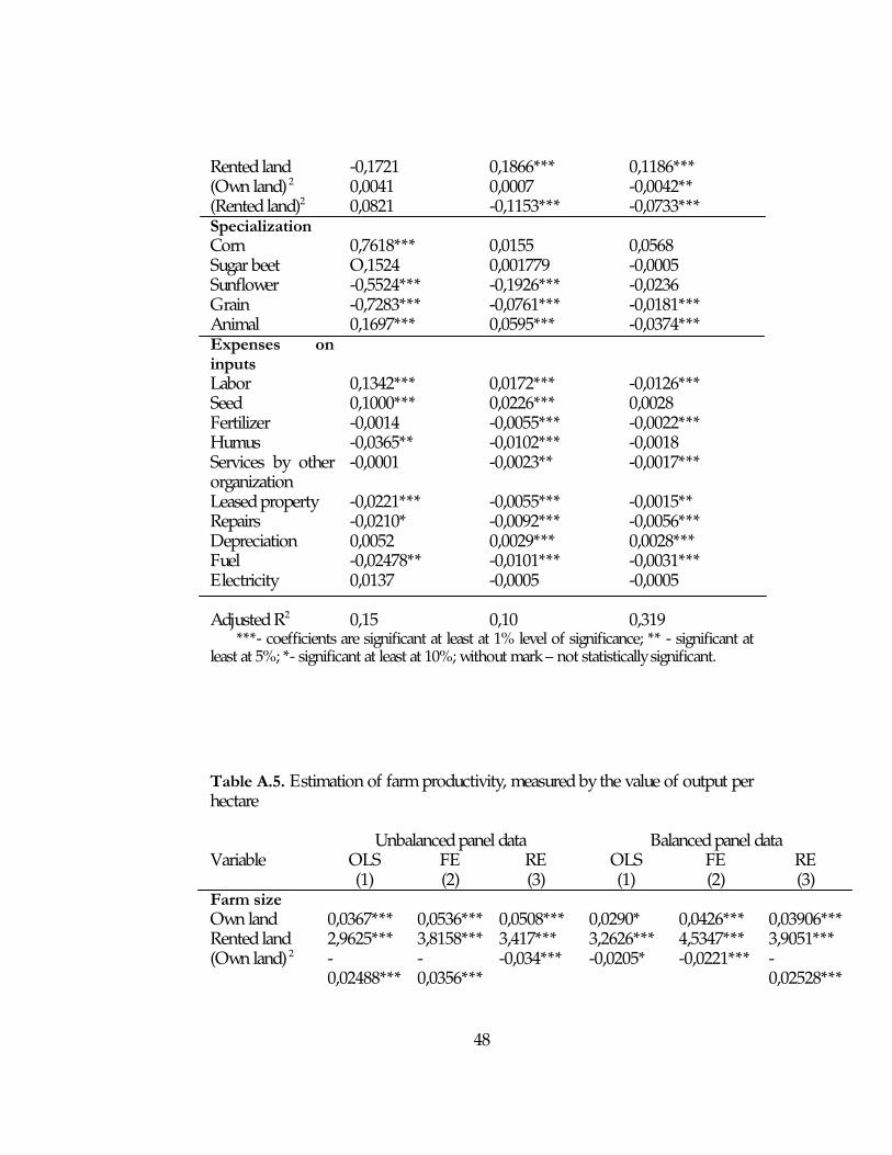
Table A.4. Second stage estimation by DEA

Variable OLS (1)

FE (3)

RE (4)

Farm size Own land 0,0251 0,0080* 0,0082***

48

Rented land -0,1721 0,1866*** 0,1186*** (Own land) 2 0,0041 0,0007 -0,0042** (Rented land)2 0,0821 -0,1153*** -0,0733*** Specialization Corn 0,7618*** 0,0155 0,0568 Sugar beet O,1524 0,001779 -0,0005 Sunflower -0,5524*** -0,1926*** -0,0236 Grain -0,7283*** -0,0761*** -0,0181*** Animal 0,1697*** 0,0595*** -0,0374*** Expenses on inputs

Labor 0,1342*** 0,0172*** -0,0126*** Seed 0,1000*** 0,0226*** 0,0028 Fertilizer -0,0014 -0,0055*** -0,0022*** Humus -0,0365** -0,0102*** -0,0018 Services by other organization

-0,0001 -0,0023** -0,0017***

Leased property -0,0221*** -0,0055*** -0,0015** Repairs -0,0210* -0,0092*** -0,0056*** Depreciation 0,0052 0,0029*** 0,0028*** Fuel -0,02478** -0,0101*** -0,0031*** Electricity 0,0137 -0,0005 -0,0005 Adjusted R2 0,15 0,10 0,319

***- coefficients are significant at least at 1% level of significance; ** - significant at least at 5%; *- significant at least at 10%; without mark – not statistically significant.

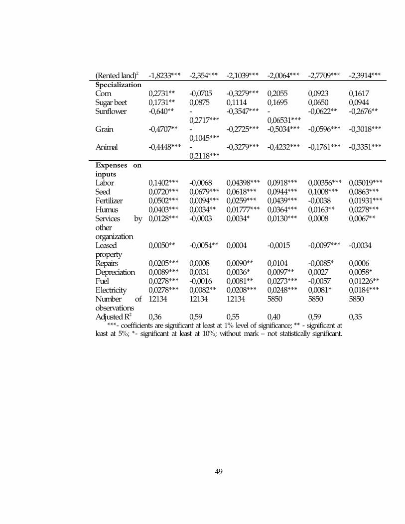
Table A.5. Estimation of farm productivity, measured by the value of output per hectare Unbalanced panel data Balanced panel data Variable OLS

(1) FE (2)

RE (3)

OLS (1)

FE (2)

RE (3)

Farm size Own land 0,0367*** 0,0536*** 0,0508*** 0,0290* 0,0426*** 0,03906*** Rented land 2,9625*** 3,8158*** 3,417*** 3,2626*** 4,5347*** 3,9051*** (Own land) 2 -

0,02488*** -0,0356***

-0,034*** -0,0205* -0,0221*** -0,02528***

49

(Rented land)2 -1,8233*** -2,354*** -2,1039*** -2,0064*** -2,7709*** -2,3914*** Specialization Corn 0,2731** -0,0705 -0,3279*** 0,2055 0,0923 0,1617 Sugar beet 0,1731** 0,0875 0,1114 0,1695 0,0650 0,0944 Sunflower -0,640** -

0,2717*** -0,3547*** -

0,06531*** -0,0622** -0,2676**

Grain -0,4707** -0,1045***

-0,2725*** -0,5034*** -0,0596*** -0,3018***

Animal -0,4448*** -0,2118***

-0,3279*** -0,4232*** -0,1761*** -0,3351***

Expenses on inputs

Labor 0,1402*** -0,0068 0,04398*** 0,0918*** 0,00356*** 0,05019*** Seed 0,0720*** 0,0679*** 0,0618*** 0,0944*** 0,1008*** 0,0863*** Fertilizer 0,0502*** 0,0094*** 0,0259*** 0,0439*** -0,0038 0,01931*** Humus 0,0403*** 0,0034** 0,01777*** 0,0364*** 0,0163** 0,0278*** Services by other organization

0,0128*** -0,0003 0,0034* 0,0130*** 0,0008 0,0067**

Leased property

0,0050** -0,0054** 0,0004 -0,0015 -0,0097*** -0,0034

Repairs 0,0205*** 0,0008 0,0090** 0,0104 -0,0085* 0,0006 Depreciation 0,0089*** 0,0031 0,0036* 0,0097** 0,0027 0,0058* Fuel 0,0278*** -0,0016 0,0081** 0,0273*** -0,0057 0,01226** Electricity 0,0278*** 0,0082** 0,0208*** 0,0248*** 0,0081* 0,0184*** Number of observations

12134 12134 12134 5850 5850 5850

Adjusted R2 0,36 0,59 0,55 0,40 0,59 0,35 ***- coefficients are significant at least at 1% level of significance; ** - significant at

least at 5%; *- significant at least at 10%; without mark – not statistically significant.